Machine learning of molecular properties: locality and active learning

Abstract

In recent years the machine learning techniques have shown a great potential in various problems from a multitude of disciplines, including materials design and drug discovery. The high computational speed on the one hand and the accuracy comparable to that of DFT on another hand make machine learning algorithms efficient for high-throughput screening through chemical and configurational space. However, the machine learning algorithms available in the literature require large training datasets to reach the chemical accuracy and also show large errors for the so-called outliers—the out-of-sample molecules, not well-represented in the training set. In the present paper we propose a new machine learning algorithm for predicting molecular properties that addresses these two issues: it is based on a local model of interatomic interactions providing high accuracy when trained on relatively small training sets and an active learning algorithm of optimally choosing the training set that significantly reduces the errors for the outliers. We compare our model to the other state-of-the-art algorithms from the literature on the widely used benchmark tests.

I Introduction

A permanent demand for the discovery of new compounds in numerous fields of industry requires development of the computational tools for prediction of molecular properties. There are many quantum-mechanical algorithms that are able to accurately predict properties of, theoretically, arbitrary atomic systems, however in practice these algorithms are too computationally expensive to be applied to a very large number of molecules. Density functional theory, which is frequently used due to its favorable trade-off between accuracy and computational cost, is still too time-consuming for high-throughput (rapid) screening of a large amount of molecules.

Machine learning (ML) algorithms are a class of algorithms that allow for fast and accurate calculations by constructing a surrogate model which “interpolates” between reference quantum-mechanical or experimental data. In particular, such models were proposed for organic molecules Browning et al. (2017); Hansen et al. (2015); Ramakrishnan et al. (2014, 2015); Ramakrishnan and von Lilienfeld (2015); Huang and Von Lilienfeld (2016); Schütt et al. (2017a); Faber et al. (2017); Gilmer et al. (2017); Huo and Rupp (2017) and they can already reach the accuracy of a few kcal/mol or lower by fitting the quantum-mechanical data. Some of the existing approaches are based on different kernels: kernels based on Coulomb matrix Rupp et al. (2012); Rupp, Ramakrishnan, and von Lilienfeld (2015), the SOAP (smooth overlap of atomic positions) kernel De et al. (2016), HDAD (histogram of distances, angles and dihedrals Faber et al. (2017)), BOB (bag of bonds Hansen et al. (2015)), BAML (bonds, angles, machine learning Huang and Von Lilienfeld (2016)), MBTR (many-body tensor representations Huo and Rupp (2017)). Other models are based on neural networks: MPNN (message passing neural networks Gilmer et al. (2017)), DTNN (deep tensor neural networks Schütt et al. (2017a)), HIP-NN (Hierarchically Interacting Particle Neural Network Lubbers, Smith, and Barros (2017)) and SchNet Schütt et al. (2017b).

In this work we propose a new algorithm of fitting of molecular properties. Our model resembles neural networks in the sense of employing several computing layers. We show that our model requires less training data to achieve the chemical accuracy when compared against the state-of-the-art approaches on the existing benchmark tests. For example, on the benchmark database consisting of 130k molecules Ramakrishnan et al. (2014) the majority of recent state-of-the-art algorithms achieve chemical accuracy only when trained on tens of thousands of samples, while our model does it with only few thousands of samples. We attribute this to our local model of interatomic interaction that effectively relates the molecular properties to the atomic environments and makes predictions for the molecules not present in the training set by accounting for contributions of the individual atomic environments.

The other problem we address with our algorithm is the issue of the so-called outliers. In the discovery of new molecules the most “interesting” molecules are often the most atypical ones. This is a challenge for ML approaches: if no molecules with similar structure are present in the training set, ML models extrapolate and commit large prediction errors for these outliers. With the proposed active learning algorithm we reduce the errors for outliers by including the molecules with the most different geometries and compositions in the training set. This prevents the cases when we are trying to predict properties of molecules that are too different from any of the training samples; instead the properties of out-of-sample molecules are interpolated by the ML model and are thus predicted accurately.

This paper has the following structure: we first formulate the problem of prediction of molecular properties in an ML framework and expose our machine-learning model. Then, in Section III we describe our active learning algorithm. In Section IV we compare our algorithm to the existing algorithms Browning et al. (2017); Hansen et al. (2015); Ramakrishnan et al. (2014, 2015); Ramakrishnan and von Lilienfeld (2015); Huang and Von Lilienfeld (2016); Schütt et al. (2017a); Faber et al. (2017); Gilmer et al. (2017); Huo and Rupp (2017) on the two benchmark datasets: QM9 Ramakrishnan et al. (2014) and QM7 Hansen et al. (2015). The concluding remarks are given in Section V.

II Machine learning model

We formulate the problem in a machine learning framework in the following way. Suppose there is a large number, $N$, of molecules whose structure (and composition) is encoded by $x^{(1)},\ldots,x^{(N)}$. The task is to construct a function $F$ that predicts a certain property (e.g., an atomization energy) of each molecule, $F(x^{(1)}),\ldots,F(x^{(N)})$. The function $F$, which we refer to as the model, will be constructed based on data—the properties of the first $n$ ($n<N$) molecules, $y^{(1)},\ldots,y^{(n)}$, which are called the labels. We will call the set $\{x^{(1)},\ldots,x^{(n)}\}$ together with $\{y^{(1)},\ldots,y^{(n)}\}$ the labeled dataset. The labeled dataset is often chosen randomly. It is a separate problem to select an optimal subset of molecules such that the prediction error for the rest of the molecules is minimized—we solve it by an active learning (or optimal experiment design) algorithm outlined in Section III. The remaining set $\{x^{(n+1)},\ldots,x^{(N)}\}$ will be called the evaluation set or the validation set. The model has a number of free parameters ${\bm{\theta}}=(\theta_{1},..,\theta_{m})$ that are found from minimizing the total loss functional

$$L({\bm{\theta}})=\sum_{j=1}^{n}\big{(}y_{j}-F\big{(}{\bm{\theta}},x^{(j)}\big{)}\big{)}^{2}\longrightarrow\min.$$ (1)

We next describe in detail the model used in the present work and its functional form $F$. We note that our testing suggests that these models do not need regularization provided that the number of parameters, $m$, is chosen significantly smaller than the number of molecules, $n$. Hence, $m$ is the only tunable hyperparameter of our model, and we found that a good rule of thumb for choosing it is $n\geqslant 2m$.

We encode a molecule by its atomic positions and types which are denoted collectively by $x$. Its molecular property (e.g., its atomization energy) is denoted by $y$ and is a function of $x$. To include our knowledge of the underlying physics into the model, we require that the representation of $y$ is invariant with respect to translation, rotation and permutation of chemically equivalent atoms in $x$.

We anticipate that some properties, such as the atomization energy or polarizability, are spatially local, i.e., depend on the local energy or polarizability of interatomic bonds. Therefore, in addition to the physical invariances, we also introduce locality in our model.

Locality

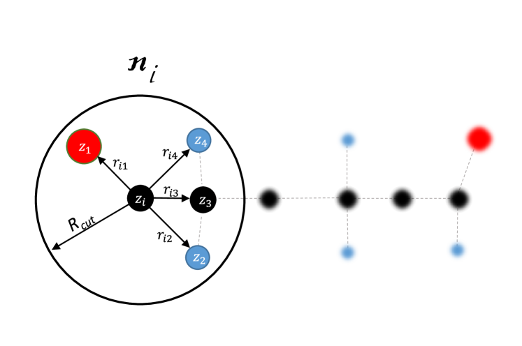
Figure 1: Neighborhood of the $i$-th atom: only the atoms within the cut-off radius $R_{\rm cut}$ interact with the central atom

We introduce locality into our model by partitioning $y$ into the sum of contributions of individual atoms. The contribution of atom $i$ depends on its atomic neighborhood: ${\mathfrak{n}}_{i}=\{(r_{ij},z_{j})\}$, where $j$ indexes all atoms within the distance $R_{{\rm cut}}$ from the atom $i$, and $r_{ij}$ and $z_{j}$ denote the radius-vectors (i.e., position of the $j$-th atom relative to the $i$-th atom) and the types of the neighboring atoms, respectively; see Figure 1 for an illustration of a neighborhood. Thus, our model is

$$F(x)=\sum_{i}V({\mathfrak{n}}_{i}).$$ (2)

Here the summation is performed over all the atoms $i$ in the molecule. Our locality assumption makes this model similar to an interatomic potential or a force field as used in molecular dynamics. This model is schematically illustrated in Figure 2. The problem thus reduces to finding the right function $V$.

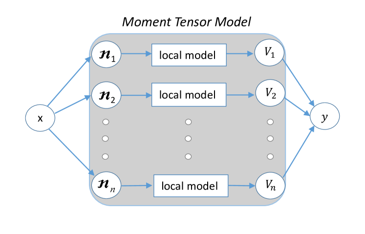
Figure 2: Partitioning scheme: a property $y$ is composed from the contributions $V_{i}$ of the individual neighborhoods ${\mathfrak{n}}_{i}$

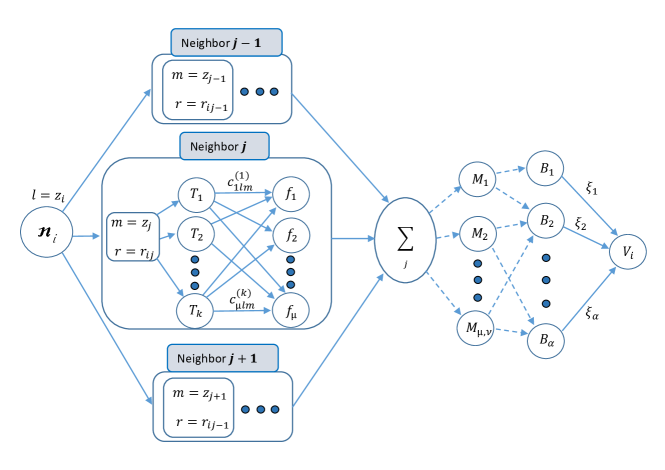
Figure 3: Computation scheme of the moment tensor model (MTM).

Moment tensors as the descriptors of atomic environment

We take $V$ as a generalization of the moment tensor potentials Shapeev (2016) to the case of several chemically different atoms. Thus, we let

$$V({\mathfrak{n}}_{i})=\sum_{\alpha}\xi_{\alpha}B_{\alpha}({\mathfrak{n}}_{i}),$$ (3)

where we call $\xi_{\alpha}$ the linear parameters, that are fitted from the data, and $B_{\alpha}({\mathfrak{n}}_{i})$ are the basis functions which we describe below. To define the basis functions, we choose a cut-off radius $R_{\rm cut}$ and introduce, as described below, a representation of the neighborhoods which is invariant with respect to rotations and permutations of chemically equivalent atoms. We note that the translation invariance is already built into (2).

We represent atomic environments using the so-called moment tensor descriptors of the following form:

$$M_{\mu,\nu}({\mathfrak{n}}_{i})=\sum_{j}f_{\mu}(|r_{ij}|,z_{i},z_{j})\underbrace{r_{ij}\otimes...\otimes r_{ij}}_{\text{$\nu$ times}},$$ (4)

where the index $j$ goes through all the neighbors of atom $i$. The symbol “$\otimes$” stands for the outer product of vectors, thus in (4) $r_{ij}\otimes...\otimes r_{ij}$ is the tensor of rank $\nu$. This way, each descriptor in (4) is composed of the radial part $f_{\mu}(|r_{ij}|,z_{i},z_{j})$ which depends only on the relative distances between atoms and on their chemical types, and the angular part $r_{ij}\otimes...\otimes r_{ij}$ resembling the moments of inertia. Indeed, if in (4) we set $f_{\mu}=m^{*}(z_{j})=m_{j}$, where $m_{j}$ is the mass of atom of type $j$ and take values of $\nu$ equal to 0, 1 and 2 we will get the descriptors $M_{\mu,0}({\mathfrak{n}}_{i})=\sum_{j}m_{j}$, $M_{\mu,1}({\mathfrak{n}}_{i})=\sum_{j}m_{j}r_{ij}$ and $M_{\mu,2}({\mathfrak{n}}_{i})=\sum_{j}m_{j}r_{ij}\otimes r_{ij}$, having a form resembling the mass, scaled center of the mass, and tensor of inertia of the neighborhood of atom $i$, respectively. Note that by construction $M_{\mu,\nu}({\mathfrak{n}}_{i})$ are invariant with respect to rotations (in a tensorial sense) and permutations of chemically equivalent atoms. It should be emphasized that $M_{\mu,0}$ are the standard two-body descriptors of atomic environments that do not contain information about angles between bonds. The general moment tensor descriptors $M_{\mu,\nu}$ remain two-body and thus offer an alternative way of including the angular information—the traditional way is to include at least three-body descriptors.

The descriptors $M_{\mu,\nu}$ defined above are tensors of different ranks. We hence define the basis functions as all possible contractions of these tensors to a scalar, for example:

$$B_{0}({\mathfrak{n}}_{i}) =M_{0,0}({\mathfrak{n}}_{i}),$$

$$B_{1}({\mathfrak{n}}_{i}) =M_{0,1}({\mathfrak{n}}_{i})\cdot M_{0,1}({\mathfrak{n}}_{i}),$$

$$B_{2}({\mathfrak{n}}_{i}) =M_{0,0}({\mathfrak{n}}_{i})(M_{0,2}({\mathfrak{n}}_{i}):M_{0,2}({\mathfrak{n}}_{i})).$$

Note that all the functions $B_{\alpha}({\mathfrak{n}}_{i})$ constructed this way are rotation invariant. The basis functions $B_{\alpha}$ resemble invariant polynomials of the atomic positions $r_{ij}$ (if the radial functions $f_{\mu}(|r_{ij}|,z_{i},z_{j})$ were polynomials of $r_{ij}$ then $B_{\alpha}$ would have been polynomials). We therefore define a level of $M_{\mu,\nu}$ by ${\color[rgb]{0.7,0,0}{\rm lev}}M_{\mu,\nu}=2\mu+\nu$ and if $B_{\alpha}$ is obtained from $M_{\mu_{1},\nu_{1}}$, $M_{\mu_{2},\nu_{2}}$, …, then ${\color[rgb]{0.7,0,0}{\rm lev}}B_{\alpha}=(2\mu_{1}+\nu_{1})+(2\mu_{2}+\nu_{2})+\ldots$. In practice we obtain different models by including all basis functions such that ${\color[rgb]{0.7,0,0}{\rm lev}}B_{\alpha}\leq d$. We then denote such a model by MTM_d (moment tensor model of level $d$). The larger the level is, the more parameters $\xi_{\alpha}$ it has.

The radial functions $f_{\mu}$ from (4) are represented in the following way:

$$f_{\mu}(r,z_{i},z_{j}) \phantom{:}=\sum_{k}c^{(k)}_{\mu,z_{i},z_{j}}Q^{(k)}(r),\qquad\text{where}$$ (5)

$$Q^{(k)}(r) :=T_{k}(r)(R_{{\rm cut}}-r)^{2}.$$

Here $T_{k}(r)$ are the Chebyshev polynomials on the interval $[R_{\min},R_{{\rm cut}}]$ and the term $(R_{{\rm cut}}-r)^{2}$ is introduced to ensure a smooth cut-off to 0. Taking into account that in real atomic systems atoms never stay too close to each other, we can always, in practice, choose some minimal distance $R_{\min}$.

The point that makes this model different from the single-component moment tensor potentials Shapeev (2016) is that now there is a dependence of the radial functions $f_{\mu}$ on the type of the central atom $z_{i}$ and the types of the other atoms in the neighborhood $z_{j}$. This dependence is encoded in the $c^{(k)}_{\mu,z_{i},z_{j}}$ coefficients. Together with $\xi_{\alpha}$ from (3) they form the set of model parameters ${\bm{\theta}}=\big{(}\xi_{\alpha},c^{(k)}_{\mu,z_{i},z_{j}}\big{)}$ that are found during the fitting procedure, see Figure 3.

For the case of single-component systems it was proved in Ref. Shapeev, 2016 that the moment tensor descriptors form a complete set of descriptors, in the sense that any function of a local atomistic environment can be approximated by a polynomial of the descriptors. It is hence easy to see that the same property holds for the multi-component systems: since the radial functions $f_{\mu}$ have an arbitrary dependence on the types of the neighboring atoms, the moments $M_{\mu,\nu}$ can describe the way atoms of type one, two, etc., are placed around the $i$-th atom independently of the other types of atoms. Since the description of each atomic type in the neighborhood is complete, the description of the entire neighborhood is complete.

Intensive quantities

To further include the knowledge of physics/chemistry into our model, we distinguish between intensive and extensive quantities. An extensive quantity (such as the atomization energy) scales with the number of atoms, while an intensive quantity (such as the HOMO/LUMO level) remains of the same order when the number of atoms in a molecule increases. The above description of the model is valid for extensive quantities, while for an intensive quantity we modify the partition relation (2) as

$$F(x)=\frac{1}{\#(x)}\sum_{i}V({\mathfrak{n}}_{i}),$$ (6)

where $\#(x)$ is the number of atoms in $x$.

A nonlocal model

To go beyond the locality assumption (2), we include nonlocal effects by introducing two different local models $V_{1}$ and $V_{2}$ (each with its own set of parameters) and let

$$v_{1} =\sum_{i}V_{1}({\mathfrak{n}}_{i}),\qquad\text{and}$$

$$v_{2} =\sum_{i}V_{2}({\mathfrak{n}}_{i}).$$

We then define the nonlocal model nlMTM in the following form

$$F_{\rm nl}(x) =p_{1}v_{1}+p_{2}v_{2}+p_{3}v^{2}_{1}+p_{4}v_{2}^{2}+p_{5}v_{1}v_{2}$$

$$\quad+p_{6}v_{1}^{3}+p_{7}v_{2}^{3}+p_{8}v_{1}^{2}v_{2}+p_{9}v_{1}v_{2}^{2}.$$ (7)

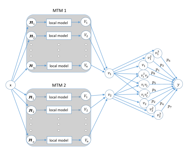
Figure 4: The nonlocal model, nlMTM, constructed from the two local models. $p_{1},\ldots,p_{9}$ are the additional fitting parameters.

Figure 4 shows how the parameters $p_{i}$ form the additional computing “layer”, if compared to the local model in Figure 2 and extend the set of parameters, ${\bm{\theta}}=\big{(}\xi_{\alpha},c^{(k)}_{\mu,z_{i},z_{j}},p_{i}\big{)}$, that are found in the training process. Such a model architecture is motivated by the fact that molecular orbitals depend largely on local environments described by several $V_{i}$ (although we only considered $i=1,2$). However, these orbitals get occupied by electrons not independently of each other, hence we assume a nonlinear dependence of the answer on the local features (7).

III Active Learning

The accuracy of prediction depends not only on the machine learning model but also on the training set that is used for the fitting. On the one hand, the size of the training set is typically limited by the amount of experiments or ab initio calculations we can conduct. On the other hand, the training set should represent the full variety of molecules to prevent extrapolation while the evaluation of molecular properties. It has been shown Huang and von Lilienfeld (2017) that an optimal choice of the training set of a fixed size can, in principle, significantly reduce the out-of-sample errors, if we were allowed to use the labels ($y^{(i)}$) of all the available data. However, a practical selection algorithm needs to choose the molecules for the training set based only on the unlabeled data ($x^{(i)}$), since in practice we want to compute the labels only after selection. The approaches related to the construction (or selection) of an optimal training set are known as active learning approaches.

Recently an approach for active learning of interatomic potentials with a linear dependence on the model parameters has been proposed Podryabinkin and Shapeev (2016). This approach is based on a D-optimality criterion for selecting the training dataset, which is equivalent to choosing atomistic configurations maximizing the determinant of the matrix of the linear equations on the model parameters. This algorithm effectively detects samples on which the model extrapolates. Hence, training on such samples prevents extrapolation and thus ensures reliable treatment of the remaining molecules at the evaluation stage.

III.1 Generalized D-optimality criterion

The model proposed in this paper has a nonlinear dependence on its parameters ${\bm{\theta}}$. Therefore we propose a generalization of the D-optimality criterion to the nonlinear case. To that end, we assume that the values of the parameters $\bar{{\bm{\theta}}}$, which are found from the training procedure (Section II) are already near the optimal ones and we hence linearize each term in the loss function (1) with respect to the parameters:

$$y^{(i)}-F\big{(}{\bm{\theta}},x^{(i)}\big{)}\approx y^{(i)}-\sum_{j}(\theta_{j}-\bar{\theta}_{j})\,\frac{\partial F}{\partial\theta_{j}}\big{(}\bar{{\bm{\theta}}},x^{(i)}\big{)}.$$

We can then interpret the fitting as the solution of the following overdetermined system of equations with respect to $\theta_{j}$:

$$\sum_{j=1}^{m}\theta_{j}\frac{\partial F}{\partial\theta_{j}}\big{(}\bar{{\bm{\theta}}},x^{(i)}\big{)}=y^{(i)}+\bar{\theta}_{j}\frac{\partial F}{\partial\theta_{j}}\big{(}\bar{{\bm{\theta}}},x^{(i)}\big{)},$$

$$\quad i=1,\ldots,n,$$

where $n$ is the size of the labeled dataset $\{x^{(1)},\ldots,x^{(n)}\}$. The matrix of this system is a tall Jacobi matrix

$${\mathsf{B}}=\begin{pmatrix}\frac{\partial F}{\partial\theta_{1}}\big{(}\bar{{\bm{\theta}}},x^{(1)}\big{)}&\ldots&\frac{\partial F}{\partial\theta_{m}}\big{(}\bar{{\bm{\theta}}},x^{(1)}\big{)}\\ \vdots&\ddots&\vdots\\ \frac{\partial F}{\partial\theta_{1}}\big{(}\bar{{\bm{\theta}}},x^{(n)}\big{)}&\ldots&\frac{\partial F}{\partial\theta_{m}}\big{(}\bar{{\bm{\theta}}},x^{(n)}\big{)}\\ \end{pmatrix},$$

where each row corresponds to a particular molecule from the training set.

Next, we select for training a subset of molecules yielding the most linearly independent rows in $B$. This is equivalent to finding a square $m\times m$ submatrix ${\mathsf{A}}$ of maximal volume (i.e., with maximal value of $|{\rm det}({\mathsf{A}})|$). We do it by using the so-called maxvol algorithm Goreinov et al. (2010).

Active learning allows us not only to extract a D-optimal training set from the labeled dataset, but also (probably, equally importantly) to estimate, at the evaluation stage, the novelty of molecules compared to those in the training set. If some molecule $x^{*}$ significantly differs from all other molecules in the training set then its properties cannot be reliably calculated. Therefore it should be labeled and added to the training set instead.

We define the “novelty” grade $\gamma(x^{*})$ as the maximal factor by which $|{\rm det}({\mathsf{A}})|$ can grow if $x^{*}$ is added to the training set. According to Ref. Goreinov et al., 2010 it can be calculated as

$$\gamma(x^{*})=\max_{1\leq j\leq n}(|c_{j}|),$$

where

$$c=\bigg{(}\frac{\partial F}{\partial\theta_{1}}\big{(}\bar{{\bm{\theta}}},x^{*}\big{)}\ldots\frac{\partial F}{\partial\theta_{n}}\big{(}\bar{{\bm{\theta}}},x^{*}\big{)}\bigg{)}{\mathsf{A}}^{-1}=:b^{*}{\mathsf{A}}^{-1}.$$

Thus, we add the molecule $x^{*}$ to the training set if $\gamma(x^{*})\geq\gamma_{\rm trsh}$, where $\gamma_{\rm trsh}\geq 1$ is a threshold parameter that prevents the algorithm from training on the molecules with not sufficiently high novelty grade $\gamma$.

Taking into account that $F(x)=\sum_{i}V({\mathfrak{n}}_{i})$, for a certain configuration $x^{(n)}$ one can write:

$$\frac{\partial F}{\partial\theta_{m}}\big{(}\bar{{\bm{\theta}}},x^{*}\big{)}=\sum_{i}\frac{\partial V({\mathfrak{n}}_{i})}{\partial\theta_{m}}\big{(}\bar{{\bm{\theta}}},x^{*}\big{)},$$

where individual atomic environments of $x^{*}$ are enumerated with $i$. Such partitioning over neighborhoods prevents an AL algorithm from selecting molecules composed from already known neighborhoods, as for such molecule the vectors $\frac{\partial V({\mathfrak{n}}_{i})}{\partial\theta_{m}}$ will be linearly dependent on such vectors of smaller molecules and thus the big molecule will not be recognized as sufficiently new one to be chosen.

III.2 Active learning scheme

We next describe our active learning procedure. It expands the training set iteratively, each time increasing its size by no more than 10%.

1. Start with a random initial training set.

2. Train the model on the current training set.

3. Using the active learning algorithm Podryabinkin and Shapeev (2016) select molecules with $\gamma\geq\gamma_{\rm trsh}$, and add either all such molecules or the molecules with the maximal $\gamma$, such that the size of the training set increases by 10% or less.

4. Unless satisfied with the current model (see the discussion below), go to step 1.

For the purpose of studying the performance of the proposed algorithm, we stopped the loop (as mentioned in step 3) when the number of molecules in the training set reached $6000$. However, in practice, other stopping criterion could be considered: the difference in accuracy of the models on two consecutive iterations on the selected (at step 2) molecules is too small. This is an intuitive criterion, however we have observed that sometimes the accuracy improvement on one particular iteration may be small, while on the next one it can increase again. Therefore, it may be better to track improvement on several iterations of the cycle.

IV Results

We have conducted a number of tests in order to clarify the following three questions: what accuracy can our model achieve on a dataset when trained on its randomly chosen subset, how the accuracy can be improved using our active learning technique (Section III), and how many training samples are required to reach the chemical accuracy, 1 kcal/mol. We remind that we use the following terminology: the training set is the set on which we train our model and the validation set consists of the full database excluding the training set. All errors quoted below are measured on the validation set.

We have tested the models of level 16, 20 and 24 denoted by MTM₁₆, MTM₂₀, MTM₂₄. The fitting of the models was done with the Broyden-Fletcher-Goldfarb-Shanno (BFGS) optimization algorithm, by performing between 2000 and 5000 iterations.

Fitting enthalpy on QM9

First, we fit our model on the so-called QM9 dataset Ramakrishnan et al. (2014) consisting of 130831 molecules formed by C,H,O,N,F atoms with up to nine heavy (C,O,N,F) atoms. This is a subset of the originally proposed database Ruddigkeit et al. (2012) consisting of 166 billion of organic molecules. The number 130831 excludes 3054 molecules from the database that failed a consistency test, as reported in Ref. Ramakrishnan et al., 2014. Following the existing works Ramakrishnan et al. (2015); Ramakrishnan and von Lilienfeld (2015); Schütt et al. (2017a); Gilmer et al. (2017); Huo and Rupp (2017) we demonstrate the performance of our method by fitting the enthalpy (or atomization energy) at 300 K.

Random choice of the training dataset

To investigate the accuracy of the MTMs with different number of parameters we have calculated the learning curves showing the dependence of the mean absolute error (MAE) on the training set size, see Figure 5. Our results are averaged over three independent random choices of the training set. As expected, the models with fewer parameters show good results for small training datasets, but are outperformed by the models with more parameters as the number of training samples grows.

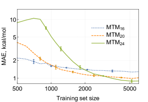
Figure 5: Random choice of the training set: dependence of MAE on the training set size. Different curves show different models: the higher is the number, the more parameters the model has.

We next compare different models by how fast (i.e., with what training dataset size) they reach chemical accuracy. Table 1 lists the prediction errors for the MTMs and the existing state-of-the-art methods when training on random training sets. While filling this table, we used MTM₁₆ for the 1k training set size, MTM₂₀ for the 3.5k training set size, and MTM₂₄ for the 10k training set size. For the sizes of 25k and 50k we used the MTM₂₈ model which has more parameters to fit then MTM₂₄. At the same time, from Fig. 5 it can be seen that using either MTM₂₀ or MTM₂₄ models still provides competitive results.

The aSLATM Huang and von Lilienfeld (2017) model reaches the chemical accuracy with the training set size about 3200, while the learning curve from Figure 5 shows that MTM₂₄ model requires almost the same number, 3500 molecules to reach such accuracy. We obtained the results for MTM₁₆, MTM₂₀, and MTM₂₄ by doing 2000 iterations of the BFGS algorithm and 5000 iterations for MTM₂₈. For a more accurate comparison with aSLATM, we trained MTM₂₄ model on 10 different random samples of training set with 3000 molecules by doing 3000 iterations of BFGS. This provided us with a validation MAE of $1.006\pm 0.0316$ kcal/mol.

As can be seen from Table 1, for training set sizes not more than 10k MTM shows a better learning curve than the existing state-of-the-art methods and only the model from the Ref. Huang and von Lilienfeld, 2017 shows nearly equal results. The works using deep NNs (Refs. Schütt et al., 2017b and Lubbers, Smith, and Barros, 2017) show better accuracy for training set sizes over 50k. Ref. Schütt et al., 2017a and Faber et al., 2017 need 25k and 35k training samples to attain the chemical accuracy, respectively. We note of another work Gilmer et al. (2017) that also reaches the chemical accuracy, but it only reports MAE of 0.55 kcal/mol while training on 110k molecules plus another 10k molecules used as a hold-out set for the early stopping criterion.

	Training set size
Model	1k	3.5k	10k	25k	35k*	50k	110k
DTNNSchütt et al. (2017a)	-	-	1.2	1.0	-	0.94	-
BAMLHuang and Von Lilienfeld (2016)	-	-	2.4	-	-	-	-
$\Delta^{B3LYP}_{MP7}-ML$Ramakrishnan and von Lilienfeld (2015)	4.8	-	3.0	-	-	-	-
MPNNGilmer et al. (2017)	-	-	-	-	-	-	0.39
HDADFaber et al. (2017)	-	-	-	-	1.0	-	0.58*
HIP-NNLubbers, Smith, and Barros (2017)	-	-	-	-	-	0.35	0.26
SchNetSchütt et al. (2017b)	-	-	-	-	-	0.59	0.31
aSLATM${}^{\cite[cite]{\@@bibref{Authors Phrase1YearPhrase2}{Huang2017opt}{\@@citephrase{(}}{\@@citephrase{)}}}}$	1.8	0.98"	-	-	-	-	-
MTM†	1.8	1.0+	0.86	0.63	-	0.41	-

Table 1: Comparison of the MAE of prediction of atomization energy (kcal/mol) by different models for different training set sizes.
^†this work
*As estimated from the graphs in Ref. Faber et al., 2017.
$+$The error can be decreased by further training, see the text.
^"as estimated from the graph in Ref. Huang and von Lilienfeld, 2017

Active learning

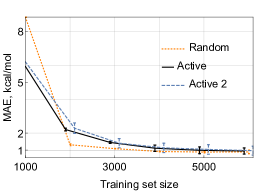
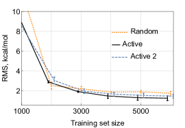
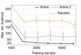
Figure 6: Active and random selection of molecules: dependencies of MAE (a), RMSE (b) and maximal error (c) on the training set size for the MTM₂₄ model.

While the MAE of MTMs trained on random training sets is small, the corresponding maximal error is of the order of 100 kcal/mol, resulting in the outliers for which the atomization energy prediction is too inaccurate. To get rid of the outliers we have applied the active learning algorithm as described in Section III. We started with a random training set of 1k molecules and it takes about 20 iterations to reach the training set size of 6k molecules. At each iteration, our training procedure takes an amount of time proportional to the training set size, while the selection always takes nearly constant time, approximately the same as required to train a model on a training set with 1k molecules.

Figure 6 shows the graphs of the MAE, RMSE and maximal absolute errors depending on the training set size, comparing random and active selection. The “Active” curve corresponds to the scenario of actively selecting molecules from the entire set of molecules and measuring the error on the remaining set. In the “Active 2” scenario we instead separate out a validation set of 30k molecules on which we measure error, while selecting and learning from the remaining 100k molecules. The error bars correspond to the 95% confidence interval as measured on three independent runs, in each of which the initial training set of 1000 molecules and the validation set in the “Active 2” scenario were random. We have used the MTM₂₄ model. It has about 2000 parameters to fit, which explains why the error on the Figure 6 exhibits overfitting when trained on less than 2000 molecules. As stated in Section II, we could improve our results for such small training set sizes by introducing regularization (which is otherwise not required).

In the active learning approach (see Section III), the training set tends to be as diverse as possible in the sense of spanning the largest volume of configurational (or molecular) space. The most extrapolative molecules lie on the boundaries of this volume and if the amount of molecules is less than or close to the number of model parameters we would not have sufficient amount of training samples in-between the boundaries. With the random selection we cover the configurational space more evenly, which results in lower RMS errors. From the part of the graph starting from 4000 training samples (this is twice the number of model parameters, as we suggested as a rule of thumb in Section II) we can see that there is no improvement in MAE (though it is rather close to the random-sampling MAE), but the RMS and maximal errors are lower that for the random sampling.

From Figure 6 it can be seen that the maximal error is much less when we are allowed to add any possible molecule to the training set (the “Active” scenario) as compared to the “Active 2” scenario, however, the error in the “Active 2” scenario is still smaller than that in random sampling. This indicates that the active learning have two mechanisms of decreasing the error: the actively chosen molecules represent better the unusual molecules in the validation set of the “Active 2” scenario, but if we are allowed to select also those unusual molecules for training, the error further drops. We argue that the latter can be useful in those applications where the region of interest in the chemical space is fixed a priori. As an example of such application, in [Nyshadham et al., 2017] the authors found six candidates of Co superalloys from about 2k a priori identified potential chemical compositions.

To better understand the impact of active learning, on Figure 8 we plotted the true and predicted enthalpies for the models trained on randomly and actively chosen training sets of 10k molecules. The plot is focused on a small region of enthalpies to show the scale of the error. As can be seen, active learning makes the error small uniformly over all the samples, while the random choice of the training set results in outliers for which the error is large.

We investigated the sizes of the molecules entering the training set at each iteration of selection (see Section III.2) and compared them to the average molecule size among the QM9 database. The results are shown on Figure 7. From this graphs it can be seen that the algorithm tries to select molecules with sizes lower than average. This could indicate that some small molecules contain representative atomic neighborhoods which occur in a many bigger molecules and the active learning algorithm detects and selects such small molecules. This result is in correspondence with the observations of Huang et al. Huang and von Lilienfeld (2017), where the authors state that an accurate model can be obtained by training on a small amount of the most relevant atomic environments (neighborhoods).

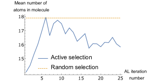
Figure 7: Mean numbers of atoms in molecule for active and random selection of configurations. The MTM₂₄ was used for this experiment.

(a) random choice of training samples

(b) active choice of training samples

Figure 8: Scatter plot of enthalpy predicted by machine learning, $H_{\rm MT}$, versus the reference enthalpy $H_{\rm ref}$, with (a) random and (b) active choice of training samples. For the illustration purposes we have plotted a small area from the whole database, where the errors are significant.

Fitting the QM7 database

Another common benchmark database we used consists of 7.2k small organic molecules with up to seven heavy atoms (C,N,O,S) saturated by H, and is referred to as QM7 montavon2013machine. We have chosen the four properties to fit: atomization energy, polarizability, and HOMO and LUMO levels. The atomization energy and polarizability are extensive quantities, and the other two are intensive quantities. The training set consisted of 5k randomly chosen molecules while the remaining 2200 were used for validation. In Table 2 we compare the accuracy of the MTMs to the other state-of-the-art methods. Our results are averaged over three independent runs. We see that the local properties, enthalpy and polarizability, are fitted with the same or higher accuracy as by the existing methods, while predictions of the HOMO and LUMO levels have a 50% larger error than the state of the art.

To address this issue, we have applied the nonlocal modification of our algorithm, nlMTM, as given by (7). From Table 2 we see that accounting for nonlocality improves the error of HOMO and LUMO to the state-of-the-art accuracy. As, the nonlocal scheme is, essentially, a three-layer model, it was found to suffer from overfitting similarly to the deep neural networks; therefore we used the early stopping technique for training the nlMTM. To that end, we used 1100 samples for estimating the error during training and measured the error on the remaining 1100 samples.

Model	$E$	$\alpha$	HOMO	LUMO
	(kcal/mol)	(Å3)	(eV)	(eV)
BAMLHuang and Von Lilienfeld (2016)	1.15	0.07	0.10	0.11
SOAPDe et al. (2016)	0.92	0.05	0.12	0.12
DTNNSchütt et al. (2017a)	1.04	-	-	-
MBTRHuo and Rupp (2017)	0.60	0.04	-	-
MTM†	0.52	0.04	0.16	0.16
nlMTM†	-	-	0.11	0.11

Table 2: Mean average errors of predicting the atomization energy $E$, polarizability $\alpha$, and HOMO and LUMO levels, committed by different models on the QM7 dataset.
^†this work

V Conclusions

We have introduced the moment tensor model (MTM) for prediction of the molecular properties based on the contributions of local atomic environments represented by the moment tensor descriptors. The accuracy of the proposed model is comparable or better than that of the state-of-the-art algorithms. The proposed model outperforms the existing algorithms by how fast it reaches the chemical accuracy on a database of 130k molecules. We attribute this to the provable completeness of our moment tensor descriptors of local environments. It should be emphasized that although our descriptors (4) are, essentially, two-body descriptors, their completeness and, in particular, angular dependence comes from their tensorial structure.

In addition, we have proposed an active learning algorithm that significantly reduces the maximal error (in other words, the error for the outliers). The algorithm effectively selects the molecules most different from those already in the training set and adds these molecules to the training set.

References

- Browning et al. (2017) N. J. Browning, R. Ramakrishnan, O. A. von Lilienfeld, and U. Roethlisberger, “Genetic optimization of training sets for improved machine learning models of molecular properties,” The Journal of Physical Chemistry Letters 8, 1351–1359 (2017).
- Hansen et al. (2015) K. Hansen, F. Biegler, R. Ramakrishnan, W. Pronobis, O. A. Von Lilienfeld, K.-R. Müller, and A. Tkatchenko, “Machine learning predictions of molecular properties: Accurate many-body potentials and nonlocality in chemical space,” The journal of physical chemistry letters 6, 2326–2331 (2015).
- Ramakrishnan et al. (2014) R. Ramakrishnan, P. O. Dral, M. Rupp, and O. A. Von Lilienfeld, “Quantum chemistry structures and properties of 134 kilo molecules,” Scientific data 1 (2014).
- Ramakrishnan et al. (2015) R. Ramakrishnan, P. O. Dral, M. Rupp, and O. A. von Lilienfeld, “Big data meets quantum chemistry approximations: the -machine learning approach,” Journal of chemical theory and computation 11, 2087–2096 (2015).