A QM/MM equation-of-motion coupled-cluster approach for predicting semiconductor color-center structure and emission frequencies

Abstract

Valence excitation spectra were computed for deep-center silicon-vacancy defects in 3C, 4H, and 6H silicon carbide (SiC) and comparisons were made with literature photoluminescence measurements. Optimizations of nuclear geometries surrounding the defect centers were performed within a Gaussian basis-set framework using many-body perturbation theory or density functional theory (DFT) methods, with computational expenses minimized by a QM/MM technique called SIMOMM. Vertical excitation energies were subsequently obtained by applying excitation-energy, electron-attached, and ionized equation-of-motion coupled-cluster (EOMCC) methods, where appropriate, as well as time-dependent (TD) DFT, to small models including only a few atoms adjacent to the defect center. We consider the relative quality of various EOMCC and TD-DFT methods for (i) energy-ordering potential ground states differing incrementally in charge and multiplicity, (ii) accurately reproducing experimentally measured photoluminescence peaks, and (iii) energy-ordering defects of different types occurring within a given polytype. The extensibility of this approach to transition-metal defects is also tested by applying it to silicon-substituted chromium defects in SiC and comparing with measurements. It is demonstrated that, when used in conjunction with SIMOMM-optimized geometries, EOMCC-based methods can provide a reliable prediction of the ground-state charge and multiplicity, while also giving a quantitative description of the photoluminescence spectra, accurate to within 0.1 eV of measurement for all cases considered.

I Introduction

Certain point defects in wide-band-gap semiconductors have been identified as promising candidates for use as qubits in quantum computing, communication, and sensing applications Neumann et al. (2008). A well-known example is the nitrogen-vacancy (NV) color center in diamond, which harbors an anionic electronic structure [(NV)^-] with well-defined $S=1$ spin states that have been initialized and coherently manipulated using optical or microwave radiation Doherty et al. (2013). The resulting stimulated emission, occurring between the ³A₂ ground state and the ³E excited state, produces a tunable photoluminescence, polarized according to an applied external magnetic field. The demonstration of long spin-coherence times at room temperature established (NV)^- centers as one of the most stable, efficient, high-quality single-photon sources known Castelletto et al. (2014); Christle et al. (2015); Widmann et al. (2015). However, diamond has inherent engineering limitations and, as a result, defects with similar properties are being eagerly sought out, both in other solid-state materials Aharonovich et al. (2016) and in nano-materials He et al. (2017).

The most closely related material to diamond in terms of $sp^{3}$ bonding is silicon carbide (SiC), and its anionic silicon-vacancy (V${}_{\mathrm{Si}}^{-}$) defects are arguably better qubit candidates than the diamond (NV)^- defect. The SiC V${}_{\mathrm{Si}}^{-}$ defects, characterized by a ⁴A${}_{2}\rightarrow{}^{4}$E transition Soykal et al. (2016), have several superior properties: they exhibit no luminescence intermittency or ‘blinking’ Bradac et al. (2010); Widmann et al. (2015), they are a half-integer $S=\frac{3}{2}$ spin (thus Kramers theorem holds) Doherty et al. (2012); Levchenko et al. (2015), and they are intrinsic defects, which do not require doping and can therefore be more easily created (e.g., using a transmission electron microscope Steeds et al. (2002), a focused ion beam WZZ (2017), ion implantation Wang et al. (2017a), etc.), as reported in Ref. Radulaski et al. (2017), where a scalable array of single silicon vacancy centers was realized Radulaski et al. (2017). Furthermore, the bulk material properties of SiC make it more amenable than diamond to high-voltage, high-power, and high-temperature applications and it is also more promising as a long-term candidate material due to its physical durability Kimoto and Cooper (2014), engineering flexibility Falk et al. (2013), and increasingly inexpensive manufacturing cost Horowitz et al. (2017); Wang et al. (2017b). One disadvantage is that the optically detected magnetic resonance of V${}_{\mathrm{Si}}^{-}$ SiC has a lower visibility compared to that of the (NV)^- center in diamond, but this too is being overcome Nagy et al. (2017).

Diamond (NV)^- and SiC V${}_{\mathrm{Si}}^{-}$ defects emit in a region of the infrared which is non-ideal for utilizing existing singlemode fiber-optic infrastructure. Recent telecommunications systems use wavelength-division multiplexing, which can use the full range of wavelengths between 1260 and 1670 nm (or 0.74 and 0.98 eV), and other popular multimode and singlemode fiber implementations operate using wavelengths of 850, 1300, and 1550 nm (or 0.80, 0.95, and 1.46 eV), with the latter being associated with the transmission-optimal so-called C-band.Olbricha et al. (2017) Consequently, several other common SiC defects are also under consideration, including the neutral divacancy Castelletto et al. (2014); Seo et al. (2017), nitrogen vacancies Csóré et al. (2017); von Bardeleben and Cantin (2017), and anti-site vacancies Umeda et al. (2006); Szász et al. (2015). More promising still is the prospect of doping with transition- or heavy-metal elements Koehl et al. (2017), although it is unclear at the outset which implants will emit the desired wavelengths.

Difficulties are often encountered when using spectroscopic techniques to distinguish between different types of vacancies or screen for specific properties across a series of substitutional defects, presenting a great opportunity for computational modeling. Modeling photoluminescence spectra requires determination of the nuclear geometry of the solid-state defect, followed by generation of accurate wave-functions for both the ground and excited states. Oftentimes acceptable geometries can be obtained for weakly correlated materials using density functional theory (DFT) methods in a plane-wave basis, and its computational scaling, usually $\mathscr{N}^{3}$–$\mathscr{N}^{4}$ with the system size $\mathscr{N}$, offers a realtively inexpensive framework. Unfortunately, problems arise when extending DFT to excited states through the time-dependent (TD) DFT formalism (see, e.g., Refs. Marques and Gross (2004); Dreuw and Head-Gordon (2005); Laurent and Jacquemin (2013); Adamo and Jacquemin (2013); Maitra (2017) for reviews). Alternatively, studies conducted in a plane-wave basis may apply the many-body $GW$ approximation Aryasetiawan and Gunnarsson (1998), sometimes even in conjunction with DFT-optimized structures Bruneval and Roma (2011), in order to gain access to band structure or excited states. The $GW$ approximation provides much more accurate results, but it also has well-known fundamental limitations: to name a few, it suffers from self-consistency errors and the route toward an exact theory is unclear.

Among the most accurate general-purpose ab initio methods available are those based on the single-reference coupled-cluster (SRCC) theory for ground states and its equation-of-motion (EOM) CC extension to excited states. These methods are size-consistent and systematically improvable, but, despite recent progress toward reducing the expense of plane-wave basis SRCC/EOMCC implementations Liao and Grüneis (2016); Hummel et al. (2017), their computational scaling remains intractable for solids. An acceptable alternative for geometry optimizations is provided by the related second-order many-body perturbation theory [MBPT(2)], which has a noniterative $\mathscr{N}^{5}$ scaling, but for an accurate treatment of excitation energies EOMCC-based methods are needed. The most basic EOMCC methods, including only single and double excitations, require steep iterative $\mathscr{N}^{5}$–$\mathscr{N}^{6}$ scalings, and this makes treatment of even a single unit cell very taxing in terms of the required CPU cycles. Meanwhile explicit treatment of a supercell model with Gaussian-based ab initio methods will be impossible for many years to come, even with modernized codes.

Here a two-fold strategy is used to minimize the computational expense associated with the aforementioned accurate computational methodologies. The first step is to partition the geometry optimization into a small group of atoms significantly perturbed by introduction of the defect site, and a comparatively very large group of atoms whose environment is unchanged by introduction of the defect. The former will be treated using high-level quantum-based methods, while the latter will be treated using low-level classical-based methods. The second step is to exploit the highly-localized nature of the associated defect photoluminescence by applying accurate excited-state many-body methods to small model systems, e.g., only those few atoms directly adjacent to the defect. For over 50 years the local nature of excitations in defect solids has been used to develop approximate methods in which the total system is is subdivided into a defect subspace and a complementary crystalline region, so this is not a novel proposition.Krmhansl (1968)

The first step is realized by utilizing the surface integrated molecular-orbital molecular-mechanics (SIMOMM) method of Shoemaker et al. Shoemaker et al. (1999), which falls into the general class of quantum-mechanics/molecular-mechanics (QM/MM) hybrid methods. The SIMOMM framework imposes a less rigid treatment of the capping atoms than its predecessor, the IMOMM model of Maseras and Morokuma Maseras and Morokuma (1995), and this reduces artificial strain imposed on the QM structure. SIMOMM was originally developed for the study of surface chemical systems, and by now its utility has been demonstrated repeatedly for describing chemistry on Si and SiC surfaces Choi and Gordon (1999); Li et al. (2000); Jung et al. (2001); Choi and Gordon (2002); Choi et al. (2002); Tamura and Gordon (2003); Rintelman and Gordon (2004); Jung and Gordon (2005); Lee et al. (2005a, b). SIMOMM geometry optimizations are perfomed under the Born-Oppenheimer approximation, which in this case is based on extremely robust assumptions Lutz and Hutson (2016). The current study is the first attempt at applying SIMOMM to describe nuclear geometries of deep-center defects in semiconductors. Note that for metallic defects other, more appropriate, QM/MM methods exist (see, e.g., Refs. Choly et al. (2005) and Liu et al. (2007)).

The second step of the abovementioned procedure is also very challenging due to the nature of the electronic excitations of interest. Excitation energies of open-shell systems with high spacial symmetry are notoriously difficult to describe, and, as a result, we employ the electron-attached (EA) and ionized (IP) EOMCC methods Nooijen and Bartlett (1995a, b). These methods have been shown to be particularly accurate for describing both ground and excited states of odd-electron, open-shell molecules. In these schemes the ($N\pm 1$)-electron systems of interest are formed through application of an electron-attaching or ionizing operator to the correlated ground-state reference of a related $N$-electron system, obtained using the SRCC approach. Alternatively, if even-electron, open-shell states are desired, they can be described by the excitation-energy (EE) EOMCC method, where the usual particle-conserving operator is applied to the same correlated $N$-electron reference. This framework allows for orthogonally spin-adapted and systematically improvable calculations of the ground and excited states of $N$- and ($N\pm 1$)-electron systems mutually related by an $N$-electron correlated reference function.

Electronically excited states dominated by one-electron transitions, particularly those that correspond to one-electron transitions from non-degenerate doubly-occupied molecular orbitals (MOs) to a singly-occupied molecular orbital (SOMO), can be accurately described by the basic EE-, EA-, or IP-EOMCCSD approaches. Meanwhile, electronic transitions characterized by two- or other, more complicated, many-electron processes, require higher-than-double excitations in order to obtain reliable results. The expense of such calculations usually limits their applicability to the smallest systems, but larger systems can be efficiently treated using the active-space EE-, EA-, and IP-EOMCC variants Oliphant and Adamowicz (1991, 1992, 1993); Piecuch et al. (1993), such as those including active-space triples, i.e., EE-, EA-, and IP-EOMCCSDt Gour et al. (2005); Gour and Piecuch (2006). Here a strategically-chosen small subset of orbitals is considered that captures the largest contributions from triple excitations.

The performance of both the basic EE-, EA-, and IP-EOMCCSD methods and the active-space EA- and IP-EOMCCSDt approaches are tested here for their ability to describe solid-state SiC defect emission frequencies. The active-space methods have already been applied to small open-shell molecules Gour et al. (2005); Gour and Piecuch (2006); Hansen et al. (2011) and ionic transition-metal complexes Ehara et al. (2012), where it was demonstrated that they can provide an accurate treatment as compared to calculations employing a full treatment of triple excitations. The current study is is the first application to deep-center defects, where the resulting EOMCC excitation energies can be directly compared to photoluminescence measurements. Some TD-DFT calculations are included for comparison, but benchmarking various functionals is outside of the scope of this work so we use those deemed optimal for Si_nC_m ($n\leq m\leq 12$) molecules in Refs. Byrd et al. (2016) and Lutz et al. (see Sect. III for further details).

The goal of the present work is to develop an accurate procedure for describing emission frequencies, and we use as benchmarks the available photoluminescence spectra for the V${}_{\mathrm{Si}}^{-}$ defects in 4H- and 6H-SiC,Wagner et al. (2000) and also the chromium silicon-substitutional defect in SiC.Koehl et al. (2017) Two distinct Si-vacancy sites exist in 4H-SiC, the $k$-site and the $h$-site, and each exhibit distinct signature photoluminescence in the infrared. Meanwhile, three distinct sites exist in 6H-SiC, the $k1$- $k2$- and $h$-sites, each of which also emit in the infrared. The V${}_{\mathrm{Si}}^{-}$ defect in 3C-SiC has not been widely reported as it potentially undergoes low-temperature annealing,Schneider and Maier (1993); Itoh et al. (1997) but there is evidence it lies in the same range as V${}_{\mathrm{Si}}^{-}$ defects in the other polytypes (1.3–1.4 eV).Orlinski et al. (2003) The measured emission frequencies of each of these six defects all fall within 0.1 eV of one another, but selective resonant optical excitation is still possible, as the spectral linewidths can be as small as 2 $\mu$eV Riedel et al. (2012). A useful theory will be able to predict each frequency to an accuracy within 0.1 eV, while also giving the correct qualitative energy-ordering of closely-spaced emission frequencies.

The structure of this paper is as follows: in Sect. II the basic theory of the EOMCC methods is presented, while in Sect. III specific details are given about how the computations were performed. Sect. IV details investigations of SIMOMM convergence, qualitative and quantitative energy-ordering of states with incremental changes in charge and multiplicity, and comparison of computed excitation energies with photoluminescence measurements for various defect sites. Conclusions and directions for future research are discussed in Sect. V.

II Theory

Figure 1: Single-particle representations of several potential ground states for V_Si and their qualitative valence-orbital energy-orderings and occupations.

In this section we provide an overview of the EOM-CC methods used to describe the excitation energies of the SiC color centers. The EE-, EA-, and IP-EOMCC theories will be employed to consider relative energies of ground and excited states with varying charge and multiplicity. These EOMCC-based methods have several advantages over standard DFT and TD-DFT: they produce spin-adapted odd-electron states, they are systematically improvable, and they can be used to generate $N$- and ($N\pm 1$)-electron states of various multiplicities from a common correlated $N$-electron reference function.

In general, a wave function $|\Psi_{\mu}\rangle$, corresponding to state $\mu$ of interest, is expressed by applying a linear excitation operator $R_{\mu}$ to the ground-state SRCC wave function,

$$|\Psi_{\mu}\rangle=R_{\mu}|\Psi^{(N)}_{0}\rangle,$$ (1)

where $|\Psi_{0}\rangle=e^{T}|\Phi\rangle$ is the CC ground state wave function formulated from the many-body cluster operator $T$ and $|\Phi\rangle$ is for the EOMCC methods in this work always given by the restricted Hartree-Fock (RHF) wave function, $|\Phi\rangle=|\Phi^{\mathrm{RHF}}\rangle$. By choosing as a starting point an $N$-electron reference CC function, $|\Psi^{(N)}_{0}\rangle$, we are able to maintain commutation relations with the $S^{2}$ and $S_{z}$ operators throughout. To access both $N$- and ($N\pm 1$)-electron states, the linear excitation operator $R_{\mu}$ must be either particle-conserving, $R_{\mu}=R_{\mu}^{(N)}$, or particle-nonconserving, $R_{\mu}=R_{\mu}^{(N\pm 1)}$, respectively, for the resulting state to be a spin-eigenfunction of the Hamiltonian.

In the particle-conserving EE-EOMCC theory, excited state energies and wave functions are obtained for an $N$-electron system by applying in Eq. 1 a linear excitation operator $R^{(N)}_{\mu}$ of the form

$$R^{(N)}_{\mu} =R_{\mu,0}+R_{\mu,1}+R_{\mu,2}+\ldots$$ (2)

$$=r_{\mu,0}+\sum_{\begin{subarray}{c}a\\ i\end{subarray}}r^{i}_{a}a^{a}a_{i}+\sum_{\begin{subarray}{c}ab\\ ij\end{subarray}}r^{ij}_{ab}a^{a}a^{b}a_{j}a_{i}+\ldots$$

where $i$,$j$,$\ldots$($a$,$b$,$\ldots$) are the occupied (unoccupied) orbitals in $|\Psi^{(N)}_{0}\rangle$, $a^{p}$($a_{p}$) are the creation (annihilation) operators associated with the spin-orbital basis set ${|p\rangle}$ used in the calculations and $r^{i}_{a}$, $r^{ij}_{ab}$,$\ldots$ are the excitation amplitudes defining the many-body components of $R^{(N)}_{\mu}$, determined by diagonalizing the similarity-transformed Hamiltonian $\bar{H}=e^{-T^{(N)}}He^{T^{(N)}}$ resulting from the ground-state $N$-electron CC calculations.

In the particle-nonconserving EA- and IP-EOMCC approaches, ground- and excited-state wave functions are obtained corresponding to states with ($N-1$)- or ($N+1$)-electron open-shell systems, respectively. The corresponding electron-attaching and ionizing operators, $R^{(N+1)}_{\mu}$ and $R^{(N-1)}_{\mu}$, respectively, entering Eq. 1 are defined as

$$R^{(N+1)}_{\mu} =R_{\mu,1p}+R_{\mu,2p-1h}+R_{\mu,3p-2h}+\ldots$$ (3)

$$=\sum_{a}r_{a}a^{a}+\sum_{\begin{subarray}{c}a<b\\ j\end{subarray}}r^{j}_{ab}a^{a}a^{b}a_{j}+\sum_{\begin{subarray}{c}a<b<c\\ j>k\end{subarray}}r^{jk}_{abc}a^{a}a^{b}a^{c}a_{k}a_{j}+\ldots$$

and

$$R^{(N-1)}_{\mu} =R_{\mu,1h}+R_{\mu,2h-1p}+R_{\mu,3h-2p}+\ldots$$ (4)

$$=\sum_{a}r^{i}a_{i}+\sum_{\begin{subarray}{c}i>j\\ b\end{subarray}}r_{b}^{ij}a^{b}a_{j}a_{i}+\sum_{\begin{subarray}{c}i>j>k\\ b<c\end{subarray}}r_{bc}^{ijk}a^{b}a^{c}a_{k}a_{j}a_{i}+\ldots$$

where $r^{i}$, $r^{ij}_{b}$, $r^{ijk}_{bc}$, $\ldots$ and $r_{a}$, $r_{ab}^{j}$, $r_{abc}^{jk}$, $\ldots$ are the corresponding electron-attaching or ionizing amplitudes defining the relevant $1h$, $2h-1p$, $3h-2p$, $\ldots$ or $1p$, $2p-1h$, $3p-2h$, $\ldots$ components of $R^{(N+1)}_{\mu}$ and $R^{(N+1)}_{\mu}$, respectively, determined by diagonalizing the similarity tranformed Hamiltonian in the appropriate sector of the Fock space.

Active-space approaches represent a practical way to account for higher-than-doubly excited clusters in the CC and EOMCC equations Oliphant and Adamowicz (1991, 1992, 1993); Piecuch et al. (1993); Piecuch (2010). The idea is to sub-partition of the one-electron basis of occupied and unoccupied spin-orbitals into (i) core or inactive occupied spin-orbitals, designated as i,j,$\ldots$, (ii) active occupied spin-orbitals, designated as I,J,$\ldots$, (iii) active unoccupied spin-orbitals, designated as A,B,$\ldots$, and (iv) virtual or inactive unoccupied spin-orbitals, designated as a,b,$\ldots$. After dividing the available orbitals into one of these four categories, only active orbitals are used to define the active-space component of the EE, EA, or IP operators $R_{\mu}^{(N)}$, $R_{\mu}^{(N+1)}$, or $R_{\mu}^{(N-1)}$, respectively. As an example, the active-space EA-EOMCCSDt{$N_{u}$} approach using $N_{u}$ active unoccupied orbitals is obtained by replacing the $3p-2h$ component $R_{\mu,3p-2h}$ of the electron attaching operator $R_{\mu}^{(N+1)}$, Eq. II, by

$$r_{\mu,3p-2h}=\sum_{\begin{subarray}{c}j>k\\ {\bf A}<b<c\end{subarray}}r_{{\bf A}bc}^{jk}a^{\bf A}a^{b}a^{c}a_{k}a_{j}.$$ (5)

Assuming a small active space is chosen, there will be relatively few amplitudes $r_{{\bf A}bc}^{jk}$ defining $r_{\mu,3p-2h}$ in Eq. 5, and they will not be much more expensive to compute than the remining $1p$ and $2p-1h$ amplitudes $r_{a}$ and $r_{ab}^{j}$ that enter the ($N+1$)-electron wave functions of the active-space EA-EOMCCSDt{$N_{u}$} approach. The IP-EOMCCSDt{$N_{o}$} active-space method is formulated in an analogous way.

Figure 2: Schematic representation of the valence orbital energy levels for Cr(CH₃)₄ assuming C_3v and T_d symmetries with the former also considered with and without orbital mixing.

III Computational details

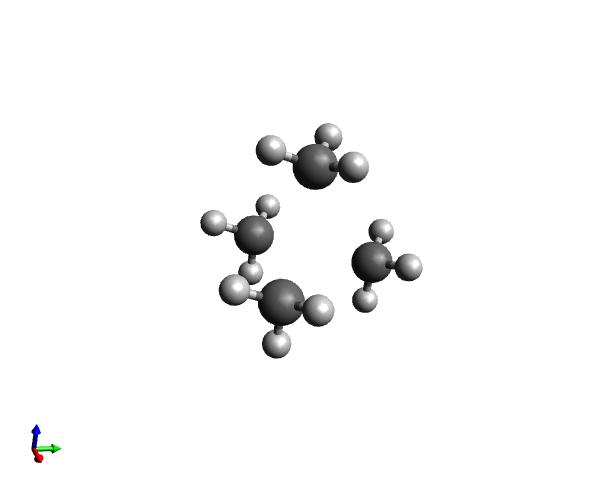
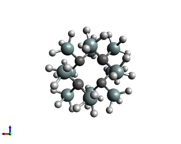
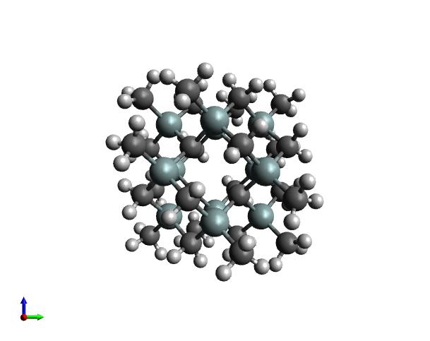
(a)                                              (b)                                              (c)

Figure 3: Atomic configurations of the QM models corresponding to the C₄H₁₂ (a), C₄Si₁₂H₃₆ (b), and C₄₀Si₁₂H₁₂₀ h-center V${}_{\mathrm{Si}}^{-}$ defect in 4H-SiC.

Here we outline necessary details for the calculations reported in Sect. IV. Supercells with perfect lattice geometries were generated using the VESTA package Momma and Izumi (2011). Perimeter C atoms were capped with hydrogens, Si atoms were capped with CH₃ groups, and defect sites were embedded into the cluster models using Avagadro and Avagadro 2 Hanwell et al. (2012). The resulting geometries were converted to the proper format for the Tinker package Ponder and Richards (1987) using OpenBabel O’Boyle et al. (2011) and for the GAMESS package M. W. Schmidt and K. K. Baldridge and J. A. Boatz and S. T. Elbert and M. S. Gordon and J. J. Jensen and S. Koseki and N. Matsunaga and K. A. Nguyen and S. Su and T. L. Windus and M. Dupuis and J. A. Montgomery, Jr. (1993); Gordon and Schmidt (2005) using MacMolPlt Bode and Gordon (1998).

Geometry optimizations are accellerated significanty by parallel implementations leveraging analytic gradients. In a previous study we have investigated the relative performance of a variety of DFT, MBPT(2), and high-level CC methods for producing geometries of several Si_nC_m ($n\leq m\leq 12$) molecules Byrd et al. (2016), which are expected to exhibit similar many-body physics to defects in solid-state SiC. The previous study found that MBPT(2) and DFT with the M11 functional were good alternatives, which could closely reproduce the geometries predicted by high-level SRCC methods. Since it is known in advance that the V${}_{\mathrm{Si}}^{-}$ defects have ⁴A₁ ground state, unrestricted (U) self-consistent field variants were employed where appropriate, i.e., UMPBT(2) and UM11. Unlike the open-shell coupled-cluster codes, both the UMBPT(2) and UM11 methods have parallel analytic gradients implemented in GAMESS Aikens and Gordon (2004), and consequently they are used here for the QM portion of optimizations. Restricted open-shell HF (ROHF) references were also tested, but convergence problems were encountered.

The T_d (C_6v) symmetry of bulk 3C- (4H- and 6H-) SiC are lowered to C_3v in the presence of vacancy defects such as V${}_{\mathrm{Si}}^{-}$. Unfortunately, the SIMOMM approach does not currently utilize the spacial symmetry of Abelian groups, as is otherwise fully implemented in GAMESS. The SIMOMM-optimized structures reported here retained an approximate C_3v symmetry, but to facilitate comparisons with other results found in the literature we had to trace back C_3v orbital labelings. Due to the lowered symmetry, an otherwise degenerate E excited state in C_3v symmetry had slightly different energies; in such cases we report the average of the two energy levels, which usually differed by a small amount (in many cases 1–5 meV). Consequently, all reported energy values are rounded to the nearest 0.01 eV, except when more decimals are needed for qualitative discussions.

Excited-state calculations were performed using the EOMCC and TD-DFT approaches, The B3LYP functional was chosen since it performed particularly well for Si_nC_m ($n\leq m\leq 12$) clusters in Refs. Lutz et al. and Boyd (2004). For TD-DFT calculations of open-shell species, only unrestricted (U) Kohn-Sham (KS) determinants were employed, as it has been advocated by Pople, Gill, and Handy that ROHF KS determinants should be avoided whenever possible Pople et al. (1995). These methods were applied to SIMOMM-optimized geometries including only the four carbon atoms immediately surrouding the defect with three capping hydrogen atoms each. Ground states are labeled with an X, while roman numerals label excited states of each symmetry, starting with 1. All computed excitation energies reported here are vertical, which is expected to be a good approximation for solid-state photoluminescence phenomena.

For EA-EOMCCSDt calculations on the V${}_{\mathrm{Si}}^{-}$ defect, a neutral CCSD reference [Fig. 1(a)] was used with active-space orbitals chosen as 5e and 15a₁ in order to construct the corresponding quartet state [Fig. 1(d)]. For the IP-EOMCCSDt calculations a doubly-anionic reference [Fig. 1(b)] was used with active-space orbitals chosen as 4e, 5e, 12a₁, and 13a₁ in order to construct the corresponding quartet state [Fig. 1(d)]. Tests including more active-space orbitals did not have a significant effect on the excitation energies of interest. The EE-EOMCCSDt method is not currently available in GAMESS, so all EE-EOMCC calculations include singles and doubles only. For EE-EOM-CCSD calculations a neutral CCSD reference [Fig. 1(a)] was used in order to construct the corresponding triplet state [Fig. 1(c)].

Table 1: Average distances ($\bar{R}$) between the h-center 4H-SiC V${}_{\mathrm{Si}}^{-}$ defect and the four surrounding atoms, with convergence of the % difference observed for various aspects of the SIMOMM model.

SIMOMM model specifications						$\Delta\bar{R}$ (% difference)
method	supercell	QM model		$\bar{R}$(Å)		QM model	MM model	basis set
UMBPT(2)/STO-3G	None	C4H12		1.814
UMBPT(2)/STO-3G	None	C40Si12H120		2.321		5.9
UMBPT(2)/STO-3G	4x4x1	C4H12		1.967			8.1
UMBPT(2)/STO-3G	4x4x1	C4Si12H36		2.038		3.5	7.1
UMBPT(2)/STO-3G	4x4x1	C40Si12H120		2.076		1.9	11.1
UMBPT(2)/STO-3G	8x8x2	C4H12		1.936			1.6
UMBPT(2)/STO-3G	8x8x2	C4Si12H36		2.005		3.5	1.6
UMBPT(2)/STO-3G	8x8x2	C40Si12H120		2.040		1.7	1.8
UMBPT(2)/CCD	None	C4H12		1.856				2.3
UMBPT(2)/CCD	None	C4Si12H36		3.895		46.5		56.1
UMBPT(2)/CCD	4x4x1	C4H12		2.013			8.1	2.3
UMBPT(2)/CCD	4x4x1	C4Si12H36		2.338		14.9	50.0	13.7
UMBPT(2)/CCD	8x8x2	C4H12		1.964			2.5	1.4
UMBPT(2)/CCD	8x8x2	C4Si12H36		1.985		1.1	16.3	1.0
UM11/CCD	8x8x2	C4Si12H36		2.004
UB3LYP/CCD	8x8x2	C4Si12H36		2.077
PBE	6x6x2	(all atoms)		2.053

When transition-metal silicon-substitutional defects are considered, the MO structure changes significantly as compared with the V_Si-type defects. As an example, the MOs of the chromium defect system are shown in Fig. 2. Starting from a T_d geometry in the non-interacting limit (Fig. 2c), an optimization will distort to a C_3v symmetry (Fig. 2b), while also hybridizing the Cr and CH₃ valence orbitals (Fig. 2a). It can be seen that for the initial T_d geometry (Fig. 2c), when an optimization is performed on the neutral ⁰Cr⁰ species all of the SOMOs can simply become doubly occupied Cr $d$ orbitals, and, in practice, this electronic configuration does not always facilitate the required orbital mixing needed for the optimization to proceed. For this reason we chose instead the ⁴Cr³⁺ state, which starts the optimization engaging the 3t₂ orbitals symmetrically. Introducing the charge draws in the CH₃ dangling bonds and initiates orbital mixing, while the quartet open-shell system can still be easily described using a single Hartree-Fock determinant.

In all QM calculations core orbitals were kept frozen, no molecular symmetry was enforced, and a spherical harmonic basis was used. For the SIMOMM optimizations, the MM partition was always treated using MM2 parameters Bowen et al. (1988), and the default maximum nuclear gradient convergence threshold was loosened to $1\text{\times}{10}^{-3}$ Hartree/Bohr, since this was shown to have a relatively small effect on the final excitation energies while reducing the number of iterations considerably. DFT and TD-DFT calculations were performed in GAMESS using a very tight grid (JANS=2). We utilize the 6-31G, 6-31G^∗, and 6-31+G^∗ basis sets Hariharan and Pople (1973); Francl et al. (1982); Clark et al. (1983); Krishnam et al. (1980); Gill et al. (1992) and the correlation-consistent basis sets of Dunning Dunning Jr. (1989); Woon and Dunning Jr. (1993); Dunning, Jr. et al. (2001). Here cc-pV$X$Z and aug-cc-pV$X$Z are abbreviated as CC$X$ and ACC$X$, respectively, where $X$ is the cardinal number of the basis set ($X$ = D, T, Q, $\ldots$). For vacancy defect calculations ghost functions were also included to improve basis set convergence. These consisted of Si functions in the specified basis set and were placed at the vacancy-defect site.

IV Results and Discussion

The primary goal of this work is to propose and validate Gaussian-based approaches for generating high-accuracy ground- and excited-state properties and energetics of vacancy and substitutional defects in semiconductors. While the procedures explored here are, in principle, systematically improvable to the exact solution, the steep computational scaling of the most accurate methods limits the scope of their application. Fortunately, photoluminescence spectra are available for benchmarking new methods and this facilitates convergence tests. Much of this study is thus devoted to identifying for use in future studies those levels of theory that offer a good compromise between accuracy and computational cost.

IV.1 Defect geometry convergence using SIMOMM

As this is the first application of SIMOMM to deep-center defects, it is important to begin by testing whether the resulting geometrical parameters converge with increasing model size. Starting from a bulk model with perfect crystal coordinates, introduction of a point defect followed by optimization with SIMOMM causes the atoms directly adjacent to the defect site to break symmetry, as Jahn-Teller distortion elongates the primary symmetry axis Prentice et al. (2017). A good single quantity to monitor for convergence is thus the average distance between the defect position and the four surrounding atoms, or $\bar{R}$. The 4H-SiC polytype was chosen for these tests because, unlike 3C-SiC, it has an anisotropic unit cell, and, unlike 6H-SiC, 4H-SiC is not too large to consider multiple concentric supercell dimensions (in integer-unit increments). While the exact geometrical structure has not been measured, prior plane-wave DFT calculations placed $\bar{R}$ close to 2.0 ÅSoykal et al. (2016). A desirable level for a convergence threshold is then a distance $\Delta\bar{R}<0.1$ Å, corresponding to $\Delta\bar{R}<5.0$% in this case.

Table 1 collects $\bar{R}$ values resulting from optimizations performed using various supercell sizes, QM model sizes, and levels of theory. When the QM model was treated at the UMBPT(2)/STO-3G level of theory with an adequate bulk MM model supercell of 128 unit cells (8x8x2), a rather large QM model size of C₄Si₁₂H₃₆ [Fig. 3(b)] was required before reaching the desired 5% convergence. Since the 252-electron C₄Si₁₂H₃₆ QM model would be computationally intractable for many accurate QM theories, this motivated us to investigate the effect of increasing the basis set size. Switching from the STO-3G to the CCD basis set improved convergence with the QM model size, and it was found that, when used with the 8x8x2 supercell, the smallest 60-electron C₄H₁₂ QM model [Fig. 3(a)], produced a $\bar{R}$ value in agreement to within 5% with the best $\bar{R}$ values reported here and in Ref. Soykal et al. (2016). The 8x8x2/C₄H₁₂ model treated at the UMBPT(2)/CCD level of theory represents the best compromise of model sizes we tested for 4H-SiC.

When a larger number of atoms are required in the QM model, DFT methods can also be used in conjunction with SIMOMM optimizations. For 4H-SiC, when the M11 functional was used in conjunction with the CCD basis set, an 8x8x2 supercell, and the C₄Si₁₂H₃₆ QM model, SIMOMM optimizations produced a $\bar{R}$ value of 2.007 Å. This value is in agreement to within 5% of our best UMBPT(2)/STO-3G result, our best UMBPT(2)/CCD result, and the literature plane-wave PBE value. Another popular functional choice, UB3LYP, was also tested and found to give a higher $\bar{R}$ value that was in good agreement with the plane-wave PBE result. These initial tests indicate that the comparatively inexpensive DFT-based SIMOMM optimizations can provide accuracies comparable to large-basis MBPT(2) calculations, though testing more functionals is outside the scope of this study.

Solid-state geometries used in the remainder of this work were optimized using SIMOMM employing the UMBPT(2)/CCD QM method and the parameters given in Table 2. Convergence tests were also performed on 3C-SiC, where improved convergence behavior was noted as compared with 4H-SiC. For the comparatively anisotropic 6H-SiC lattice, we used the largest affordable roughly-cubic supercell, having dimensions 9x9x1.4. The 3C, 4H, and 6H polytypes make an interesting case study for testing our methods, since there is varying degree of anisotropy of the unit cells with little other significant change in the environment of the defect.

IV.2 Charge and multiplicity of the ground-state

Table 2: Parameters defining the computational models

	SiC polytype
	3C	4H	6H
space group	F43m	P63mc	P63mc
$a$(Å)	4.368	3.079	3.079
$c$(Å)	—	10.07	15.12
supercell boundaries	4x4x4	8x8x2	9x9x1.4
MM crystal atoms	865	1561	1824
MM hydrogen atoms	539	955	1007
unique Si-defect sites	1	2	3
QM crystal atoms	4	4	4
QM hydrogen atoms	12	12	12

A major challenge in the study of solid-state defects and their photoluminescence spectra, assuming knowledge of the material’s polytype and the defect type, is the characterization of the electronic ground-state of the defect site in terms of its charge and multiplicity. One consequence of the high symmetry of point defects is orbital degeneracy, and, in analogy to Hund’s rule for atoms, this can lead to unusual charges and multiplicities being the most energetically favorable. Energy-ordering states related by incremental changes in charge and multiplicity can be problematic using electronic structure methods such as DFT and TD-DFT because they typically treat each case with a different SCF reference. Ideally, a method should instead build a series of states from the same correlated reference, as can be done using the EOMCC family of methods. When the appropriate level of correlation effects are included, these methods will provide a highly accurate description of energy differences between various potential ground states.

Several possible 3C-SiC V_Si ground states are illustrated in Fig. 1, where they are represented qualitatively using independent-particle-model orbital energy levels. By now there is consensus that the two most stable electronic configurations are the neutral $S=1$ state [V${}_{\mathrm{Si}}^{0}$(³A₂)] and the anionic $S=\frac{3}{2}$ state [$V_{\mathrm{Si}}^{-}$(⁴A₂)], with the latter being the ground state for all three SiC polytypes. Less is known about the relative energies of other states, e.g., V${}_{\mathrm{Si}}^{0}({}^{1}$A${}_{1})$, V${}_{\mathrm{Si}}^{2-}$(¹A₁), or V${}_{\mathrm{Si}}^{-}$(²E). Since the V${}_{\mathrm{Si}}^{0}$(³A₂) species spontaneously ionizes to form the $V_{\mathrm{Si}}^{-}$(⁴A₂) species, it must be that the additional stabilizing exchange energy produced in the anionic form is greater than the energy gained by breaking the symmetry of the t₂ orbital to form its 5e and 14a₁ components.

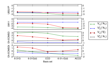
Figure 4: Relative energies (in eV) of various electronic states of V${}_{\mathrm{Si}}^{-}$ in 3C-SiC. Each value is computed using the designated method and basis set and reported with respect to the corresponding V${}_{\mathrm{Si}}^{0}$(¹A₁) energy.

Fig. 4 plots relative energies of several low-lying 3C-SiC V_Si states as a function of basis set size using the UB3LYP, UM11, EA-EOMCCSD, and EA-EOMCCSDt{3} methods. Let us first consider these results in terms of what is known. All combinations of method and basis set correctly place the ³V${}_{\mathrm{Si}}^{0}$ state below the ¹V${}_{\mathrm{Si}}^{0}$ state, but there is great variation in the quantitative difference. Beyond this, the ACCD basis set results for the UB3LYP, UM11, and EA-EOMCCSDt{3} methods also correctly place the ⁴V${}_{\mathrm{Si}}^{-}$ state lowest. Considering the remaining states, it is seen that the energy-ordering provided by the DFT and EA-EOMCCSDt{3} methods differ qualitatively and further discussion is warranted.

One potentially consequential discrepency between the DFT and EA-EOMCCSDt{3} state orderings is their relative placement of the anionic V${}_{\mathrm{Si}}^{-}$(²E) state with respect to the neutral V${}_{\mathrm{Si}}^{0}$(³A₂) and V${}_{\mathrm{Si}}^{0}$(¹A₁) states. Limiting the discussion to the ACCD basis set results in Fig. 4, the DFT methods place both anionic states lower than the neutral states, while the EA-EOMCCSDt{3} method places the V${}_{\mathrm{Si}}^{-}$(²E) state more than 2 eV higher than the V${}_{\mathrm{Si}}^{-}$(⁴A₂) state, and, importantly, also above both neutral states. Experimental realization of a Lambda system such as the one proposed in Ref. Soykal et al. (2016) based on DFT calculations, may be compromised by the possibility of system ionization during excitation or relaxation processes occurring between the V${}_{\mathrm{Si}}^{-}$(²E) and V${}_{\mathrm{Si}}^{-}$(⁴A₂) states.

Returning to comment on the basis-set dependence of the computational models, all methods presented in Fig. 4 show a significant ($>$1 eV) shift in at least one of the reported states when going from the 6-31G^∗ to 6-31+G^∗ basis sets. This demonstrates the importance of diffuse functions for the accurate energy-ordering of defect states. Both the UB3LYP and EA-EOMCCSDt methods exhibit a basis-set dependence of the state ordering, with the EA-EOMCCSDt state-ordering not completely resolved until the ACCD basis set is employed. It is thus important to use good-quality basis sets with diffuse functions when performing energy-ordering studies on minimal vacancy defect models.

Table 3: Relative energies (in eV) for the V${}_{k}^{0}({}^{1}$A${}_{1})$$\rightarrow$V${}_{k}^{-}({}^{4}$A${}_{1})$ transition, computed using various method and basis-set combinations.

UB3LYP	UM11		EA-EOMCCSD						EA-EOMCCSDt{3}							GW approx.
ACCT	ACCT		6-31G	6-31G∗	CCD	6-31+G∗	ACCD		6-31G	6-31G∗	CCD	6-31+G∗	ACCD	ACCT		plane-wave
-3.28	-4.07		3.03	3.26	2.89	1.81	1.64		0.42	-0.24	-0.75	-1.11	-1.46	-1.67		-1.58

Without benchmark values for comparison, it is difficult to draw definitive conclusions from the data in Fig. 4 about the relative accuracy of these methods. Table 3 provides a quantitative comparison of computed energy differences for the V${}_{k}^{0}$(¹A₁)$\rightarrow$V${}_{k}^{-}$(⁴A₁) transition, with a literature plane-wave-based GW-approximation value also included for comparison Bruneval and Roma (2011). The UB3LYP and UM11 DFT approaches produce relative energies over twice as large as the GW approximation, while the EA-EOMCCSD method consistently produces the wrong sign for the energy difference. The EA-EOMCCSDt{3} method fares much better. When the ACCD and ACCT basis sets are employed, EA-EOMCCSDt{3} produces values differing by only $\sim$ 0.1 eV from the $GW$ approximation. This provides supportive evidence that the EA-EOMCCSDt{3} produces the most accurate relative energetics of the four methods used here, and thus it likely also provides the most reliable state-ordering in Fig. 4.

IV.3 Basis set convergence of excitation energies

In this section we investigate the accuracy and basis-set convergence of excitation energies produced out of the V${}_{k}^{-}$(⁴A₁) state using EOMCC and TD-DFT methods. In Ref. Soykal et al. (2016) plane-wave DFT calculations were used to qualitatively order a series of doublet and quartet excited states, with symmetries predicted using a purely group-theoretic approach. It is thus an interesting question whether our Gaussian-based procedure will produce energy-ordering of excited states similar to the plane-wave DFT calculations. Before making such comparisons, in this section we establish an appropriate method and basis set for our approach through convergence tests.

Table 4 collects excitation energies generated using various methods and basis sets, with only the two lowest-lying quartet states, 1⁴A₁ and 1⁴E, reported. In terms of the basis set convergence, it is clear from Table 4 that, regardless of the method, diffuse functions are essential to the accuracy of the model. When the 6-31+G^∗ and ACCD basis sets including diffuse functions are employed, the resulting excitation energies are within 0.25 eV of the corresponding ACCT results, providing a practical alternative to ACCT in defect calculations where expense is a limiting factor. Full IP- and EA-EOMCCSDT results are also included for the 6-31G basis set; the strong similarity of the values produced by the active-space methods and their parent methods (within 0.01 eV) indicates that the active-space orbitals are an appropriate set for capturing the most important triples effects.

Table 4: Convergence of 3C-SiC excitation energies (in eV) for transitions from the V${}_{\mathrm{Si}}^{-1}$(X⁴A₁) ground state to the excited ⁴A₁ state (above) and ⁴E state (below), corresponding to orbital transitions dominated by 14a₁$\rightarrow$15a₁ and 14a₁$\rightarrow$6e character, respectively [Fig. 1(a)].

	Basis set
Method	6-31G	6-31G∗	CCD	6-31+G∗	ACCD	ACCT
UB3LYP	2.50	2.48	2.35	1.89	1.81	1.76
IP-EOMSD	7.56	7.33	6.44	3.85	2.49	2.62
IP-EOMSDt	7.61	6.10	5.07	2.97	2.88	2.91
IP-EOMSDT	5.78
EA-EOMSD	2.66	2.60	2.22	0.82	0.48	0.31
EA-EOMSDt	2.60	2.56	2.43	3.00	2.94	2.75
EA-EOMSDT	2.60
UB3LYP	2.51	2.47	2.34	1.88	1.80	1.76
IP-EOMSD	2.44	2.37	2.29	1.96	3.27	3.27
IP-EOMSDt	2.54	2.47	2.34	1.79	3.47	3.36
IP-EOMSDT	2.54
EA-EOMSD	3.04	3.09	2.23	0.22	0.06	0.14
EA-EOMSDt	3.74	4.09	3.34	1.38	1.32	1.35
EA-EOMSDT	3.73

Considering more closely the X⁴A${}_{1}\rightarrow 1{}^{4}$A₁ transition, in Table 4 a significant discrepancy is found between the excitation energies produced by the UB3LYP, EA-EOMCCSD, and EA-EOMCCSDt{3} methods. Differences between EA-EOMCCSD and EA-EOMCCSDt are attributable to the significant contributions from $r_{\mu,3p-2h}$ amplitudes (see Eqs. II and 5) found for the X⁴A₁ state. The EA-EOMCCSDt{3} and UB3LYP methods are also in disagreememnt for the same transition by nearly 1.0 eV. The EA-EOMCCSDt{3} method places the $1{}^{4}$A₁ state 1.4 eV higher in energy than the $1{}^{4}$E state, while UB3LYP predicts the two excited states to be quasi-degenerate. Since a well-known deficiency of TD-DFT is that it does not incorporate two-electron transitions, this can again be attributed to the significant $r_{\mu,3p-2h}$ amplitudes appearing in the EA-EOMCCSDt{3} calculations, which indicate that the excitation is not a pure one-electron transition. Indeed, the UB3LYP 1⁴A₁ configuration state function is dominated by one large ($>0.98$) amplitude out of the X⁴A₁ state with all other amplitudes being small ($<0.1$), indicating that there are virtually no accompanying orbital rotations.

Table 4 also includes IP-EOMCC results, as these are often more accurate than the EA-EOMCC methods if the target radical anionic ($N+1$)-electron wave function more closely resembles a doubly anionic ($N$+2)-electron species rather than the $N$-electron one. The EA-EOMCCSDt{3} and IP-EOMCCSDt{6} results converge toward a similar value for the 1⁴A₁ state, but the IP-EOMCCSD and IP-EOMCCSDt{6} results do not converge systematically for the X⁴A${}_{1}\rightarrow 1{}^{4}$E transition. In other situations the IP-EOMCC methods may be a better choice, but since the EA-EOMCC methods are a more convenient and accurate choice for these systems we focus on them here for the remainder of this study.

IV.4 Benchmarking excitation energies of silicon-vacancy defects in 4H- and 6H-SiC

Photoluminescence spectra have previously been obtained for 4H- and 6H-SiC and these can be used to benchmark the accuracy of our approach, which so far has been tested only on 3C-SiC. In Table 5 excitation energies computed with the UB3LYP/ACCT and EA-EOMCCSDt{3}/ACCD methods are compared with related photoluminescence measurements for all V${}_{\mathrm{Si}}^{-}$ defect types in 4H- and 6H-SiC. The EA-EOMCCSDt{3} computational values for the X⁴A${}_{1}\rightarrow 1^{2}$E transition are all within 0.1 eV to the measured values. The EA-EOMCCSDt{3} energy-ordering of different defect types within a given polytype also qualitatively matches with measurements, indicating this method may be helpful in future studies for distinguishing defect types differing subtly in energy. For both the 4H and 6H polytypes the X⁴A${}_{1}\rightarrow 1{}^{4}$A₁ transition is nearly 3 eV, which supports the similar assignment made for 3C-SiC in Table 4. We note that the magnitude of the error increases with increasing unit-cell anisotropy, and thus the larger errors f 6H-SiC would likely be reduced by utilizing a more complete supercell during the SIMOMM optimization.

Comparing instead the TD-DFT calculations with the measured values, somewhat erratic UB3LYP results were found for the same set of geometries. In more than one case the energies are too large by over 0.5 eV when compared to the corresponding benchmark values, and in almost all cases the $1{}^{4}$A₁ and $1{}^{4}$E states lie very close in energy, similar to what was found for 3C-SiC in Sect. IV.3. For the k2-type 6H-SiC defect, where the X⁴A${}_{1}\rightarrow 1{}^{4}$A₁ excitation energy is too small by more than 1 eV, the underlying DFT calculation has presumably converged to the 1⁴A₁ state, as evidenced by it being nearly degenerate with the $1{}^{4}$E state. Since our goal was simply to identify the most accurate methods for our procedure, we did not attempt to rotate the KS orbitals in pursuit of a lower-energy state.

Table 5: Comparison of computed and measured excitation energies (in eV) for transitions out of the $V_{\mathrm{Si}}^{-}$(⁴A₁) state in 4H- and 6H-SiC. The upper and lower tables differ only in the computational method used to generate vertical excitation energies, as indicated, while the final line provides measured values for reference.

	UB3LYP/ACCT
	4H-SiC			6H-SiC
State	k(V1)	h(V2)		k1(V1)	h(V2)	k2(V3)
V${}_{\mathrm{Si}}^{-}$($1{}^{4}$A1)	1.990	1.513		2.051	1.754	1.218
V${}_{\mathrm{Si}}^{-}$($1{}^{4}$E)	1.982	1.497		2.051	1.754	0.061
	EA-EOMCCSDt/ACCD
	4H-SiC			6H-SiC
State	k(V1)	h(V2)		k1(V1)	h(V2)	k2(V3)
V${}_{\mathrm{Si}}^{-}$($1{}^{4}$A1)	2.968	3.084		2.966	2.967	2.961
V${}_{\mathrm{Si}}^{-}$($1{}^{4}$E)	1.424	1.321		1.334	1.331	1.329
Experiment	1.438	1.352		1.433	1.398	1.368

IV.5 Chromium silicon-substitutional defects in SiC

Photoluminescence frequencies of the V${}_{\mathrm{Si}}^{-}$ defect are unsuitable for leveraging existing telecommunication technology, and there is consequently ramping interest in screening transition-metal defects for a color center with an emission frequency compatible with fiber-optic technology. While many methods struggle to accurately describe transition-metal excitation energies, the active-space EA- and IP-EOMCC methods have recently proven to be very successful for transition metals when used appropriately Bauman et al. (2016a, b). As a more challenging test of our approach, here we make a first attempt at reproducing the excitation energy for a transition-metal defect in SiC. The photoluminescence spectra for a single chromium defect in SiC has been recently measured, and the authors of Ref. Koehl et al. (2017) have reported peaks at 1.1587 and 1.1898 eV ³Cr⁴⁺ defect corresponding to the $h$- and $k$-type silicon sites of 4H-SiC, respectively.

After obtaining a converged quartet Cr³⁺(CH₃)₄ geometry for 3C-SiC, as described in Sect. III, the preferred charge and multiplicitly of the ground state was investigated using EE-EOMCCSD and EA-EOMCCSDt calculations. Our initial exploratory calculations were performed using the 3C polytype of SiC because we encountered convergence problems for Cr-embedded 4H-SiC. From the results presented in Table 6 it can be seen that calculations performed at all reported basis set levels place the Cr${}_{\mathrm{Si}}^{0}({}^{3}$A${}_{2})$ species lowest in energy. In this case there is no change in the energy-ordering of states with increasing basis set, and, as in Sect. IV.2, ground-state energy differences computed using the ACCD basis set appear adequately converged. This agrees with the ground-state multiplicity predicted in Ref. Koehl et al. (2017), but the oxidation state differs from the 4+ oxidation state reported there (presumably their value corresponds to the oxidation number of the source material). A Mulliken population analysis confirms the predicted oxidation state is close to zero, producing a value of 0.15 a.u. on the Cr atom when the ACCD basis set is used.

In Ref. Koehl et al. (2017) the authors posited that the observed 4H-SiC Cr${}_{\mathrm{Si}}^{0}$ transition is due to a X³A${}_{2}\rightarrow 1{}^{1}$A₁ transition. Our 3C-SiC result for that transition is 1.15 eV, in good agreement with the measured 4H-SiC values. Of further interest are the result of our calculation for the 3C-SiC Cr${}_{\mathrm{Si}}^{0}$ X³A${}_{2}\rightarrow 1{}^{3}$A₂ transition, which yielded a value of 1.44 eV. This transition is close enough to the fiberoptic C-band that it may be worth further consideration, especially since these defects can already be reliably created and measured.

Table 6: Relative energies of chromium-defect states of incremental charge and multiplicity. Energies were computed using the EE-EOMCCSD/ACCD and EA-EOMCCSDt/ACCD method for systems with an even and odd numbers of electrons, respectively. All values are reported relative to the neutral singlet Cr${}_{\mathrm{Si}}^{0}({}^{1}A_{1})$ state, in eV.

Species(state)	6-31G	6-31+G∗	ACCD
Cr${}_{\mathrm{Si}}^{2-}({}^{1}$A${}_{1})$	6.92	4.04	N/C
Cr${}_{\mathrm{Si}}^{-}({}^{2}$E$)$	0.11	-0.49	0.27
Cr${}_{\mathrm{Si}}^{0}({}^{3}$A${}_{2})$	-1.37	-1.24	-1.15
Cr${}_{\mathrm{Si}}^{+}({}^{2}$E$)$	4.86	5.24	5.49
Cr${}_{\mathrm{Si}}^{+}({}^{4}$E$)$	6.97	7.47	7.81
Cr${}_{\mathrm{Si}}^{2+}({}^{1}$A${}_{1})$	19.01	19.39	19.63
Cr${}_{\mathrm{Si}}^{2+}({}^{3}$A${}_{2})$	19.27	19.77	20.03
Cr${}_{\mathrm{Si}}^{3+}({}^{2}$E$)$	38.55	N/C	N/C
Cr${}_{\mathrm{Si}}^{4+}({}^{1}$A${}_{1})$	65.07	N/C	N/C
Cr${}_{\mathrm{Si}}^{4+}({}^{3}$A${}_{2})$	64.40	N/C	N/C

V Conclusions

In this study we proposed and validated an ab initio Gaussian-based method for predicting the structure and emission frequencies of deep-center defects in semiconductors. The procedure is as follows: starting from perfect crystalline lattice coordinates, the defect is introduced and the positions of the surrounding atoms are optimized using the QM/MM method SIMOMM. Excitation energies are then computed by applying highly-accurate EOMCC-based methods to a model structure consisting of several atoms immediately adjacent to the defect, in their SIMOMM-optimized positions. While these minimal model geometries were sufficient to produce excitation energies comparable to the corresponding photoluminescence measurements, it should also be emphasized that the steep expense of EOMCC methods are being overcome, both through massively-parallel computing algorithms Lotrich et al. (2008); Brabec et al. (2011) and orbital localization schemes Flocke and Bartlett (2004); Auer and Nooijen (2006); Li et al. (2009); Eriksen et al. (2015); Liakos and Neese (2015). After breaking free of the associated intractable computational scalings, the systematically improvable nature inherent to our SIMOMM-based method will be a critical advantage over plane-wave methods.

It was demonstrated through convergence tests that the Gaussian-based QM/MM method SIMOMM could achieve a similar level of accuracy to plane-wave based PBE calculations using around 1000 atoms in the bulk MM model. With the QM portion sufficiently constrained, and assuming that an adequately large basis set was employed, both MBPT(2) and DFT with the M11 functional were shown to provide accurate geometries with a QM treatment of only the four carbon atoms immediately adjacent to the defect center. Given as a starting point these accurate optimized geometries, EOMCC-based methods were shown to be powerful tools for the prediction of the electronic structure of defect centers. Using a sufficiently large basis set, the EA-EOMCCSDt method reliably predicted the ground state for silicon-vacancy defects among several states varying in charge and multiplicity, and it produced quantitative excitation energies, always in agreement with photoluminescence measurements to within 0.1 eV.

After establishing the accuracy of this procedure on silicon-vacancies in SiC, a first attempt was made to apply it to a chromium silicon-substitutional defect and EOMCC-based methods were successful there, too. For 3C-SiC, EE-EOM-CCSD was able to correctly predict a triplet ground state and a related excitation energy closely comparable to the recently measured 4H-SiC photoluminescence spectrum. Our calculations predicted the chromium ground-state to have a zero oxidation number however, in disagreement with Ref. Koehl et al. (2017) which assumed a +4 Cr oxidation state.

The computational procedure developed here will facilitate efficient screening of defect emission frequencies that would otherwise take years to create and measure in the laboratory. This method is broadly applicable to various defects in SiC and other semiconductors, and we will use it in a subsequent study to screen many candidate defects, including transition-metal substitutional defects other than Cr, in pursuit of one that emits in a region compatible with the exisiting fiber-optic infrastructure. Fabrication of such a device would go a long way toward establishing the silicon-photonic route as the leading candidate platform for the realization of quantum information networks.

VI Acknowledgements

The views expressed in this work are those of the authors and do not reflect the official policy or position of the United States Air Force, Department of Defense, or the United States Government. The DoD High Performance Computing Modernization (HPCMO) Program and the AFRL Supercomputing Resource Center (DSRC) are gratefully acknowledged for financial resources and computer time and helpful support. This work was sponsored by a HASI grant from HPCMO and a joint AFRL/AFIT grant awarded at the AFRL Director’s authority. This project was enabled in part by an appointment to the Internship/Research Participation Program at the Air Force Institute of Technology, administered by the Oak Ridge Institute for Science and Education through an interagency agreement between the U.S. Department of Energy and EPA.

References

- Neumann et al. (2008) N. Neumann, F. Mizuochi, P. Rempp, H. Hemmer, S. Watanabe, S. Yamasaki, V. Jacques, T. Gaebel, F. Jelezko, and J. Wrachtrup, Science 320, 1326 (2008).
- Doherty et al. (2013) M. W. Doherty, N. B. Manson, P. Delany, F. Jelezko, J. Wrachtrup, and L. C. L. Hollenberg, Phys. Rep 528, 1 (2013), doi:10.1016/j.physrep.2013.02.001.
- Castelletto et al. (2014) S. Castelletto, B. C. Johnson, V. Ivády, N. Stavrias, T. Umeda, A. Gali, and T. Ohshima, Nat. Mater. 13, 151 (2014).
- Christle et al. (2015) D. J. Christle, A. L. Falk, P. Andrich, P. V. Klimov, J. U. Hassan, N. T. Son, E. Janzén, T. Ohshima, and D. D. Awschalom, Nat. Mater. 14, 160 (2015).
- Widmann et al. (2015) M. Widmann, S.-Y. Lee, T. Rendler, N. T. Son, H. Fedder, S. Paik, L.-P. Yang, N. Zhao, S. Yang, I. Booker, A. Denisenko, M. Jamali, S. A. Momenzadeh, I. Gerhardt, T. Ohshima, A. Gali, E. Janzén, and J. Wrachtrup, Nat. Mater. 14, 164 (2015).
- Aharonovich et al. (2016) I. Aharonovich, D. Englund, and M. Toth, Nat. Photonics 10, 631 (2016).
- He et al. (2017) X. He, N. F. Hartmann, X. Ma, Y. Kim, R. Ihly, J. L. Blackburn, W. Gau, J. Kono, Y. Yomogida, A. Hirano, T. Tanaka, H. Kataura, H. Htoon, and S. K. Doorn, Nat. Photonics (2017).
- Soykal et al. (2016) Ö. O. Soykal, P. Dev, and S. E. Economou, Phys. Rev. B 93, 081207 (2016).
- Bradac et al. (2010) C. Bradac, T. Gaebel, N. Naidoo, M. J. Sellars, J. Twamley, L. J. Brown, A. S. Barnard, T. Plakhotnik, A. V. Zvyagin, and J. R. Rabeau, Nat. Nanotechnol. 5, 345 (2010).
- Doherty et al. (2012) M. W. Doherty, F. Dolde, H. Fedder, F. Jelezko, J. Wrachtrup, N. B. Manson, and L. C. L. Hollenberg, Phys. Rev. B 85, 205203 (2012), doi:10.1103/Phys-RevB.85.205203.
- Levchenko et al. (2015) A. O. Levchenko, V. V. Vasil’ev, S. A. Zibrov, A. S. Zibrov, A. V. Sivak, and I. V. Fedotov, Appl. Phys. Lett. 106, 102402 (2015), doi:10.1063/1.4913428.
- Steeds et al. (2002) J. Steeds, G. Evans, L. Danks, and S. Furkert, Diamond Relat. Mater. 11, 1923 (2002), doi:10.1016/S0925-9635(02)00212-1.
- WZZ (2017) ACS Photonics 4, 1054 (2017).
- Wang et al. (2017a) J. Wang, Y. Zhou, X. Zhang, F. Liu, Y. Li, K. Li, Z. Liu, G. Wang, and W. Gao, Phys. Rev. Applied 7, 064021 (2017a).
- Radulaski et al. (2017) M. Radulaski, M. Widmann, M. Niethammer, J. L. Zhang, S.-Y. Lee, T. Rendler, K. G. Lagoudakis, N. T. Son, E. Janzén, T. Ohshima, J. Wrachtrup, and J. Vučković, Nano Lett. 17, 1782 (2017).
- Kimoto and Cooper (2014) T. Kimoto and J. A. Cooper, Fundamentals of Silicon Carbide Technology: Growth, Characterization, Devices, and Applications (Wiley, Singapore, 2014) pp. 11–38.
- Falk et al. (2013) A. L. Falk, B. B. Buckley, G. Calusine, W. F. Koehl, V. V. Dobrovitski, A. Politi, C. A. Zorman, P. X.-L. Feng, and D. D. Awschalom, Nat. Comm. 4, 1819 (2013).
- Horowitz et al. (2017) K. Horowitz, T. Remo, and S. Reese, A Manufacturing Cost and Supply Chain Analysis of SiC Power Electronics Applicable to Medium-Voltage Motor Drives, Tech. Rep. TP-6A20-67694 (National Renewable Energy Laboratory, 2017).
- Wang et al. (2017b) L. Wang, Q. Cheng, H. Qin, Z. Li, Z. Lou, J. Lu, J. Zhang, and Q. Zhou, Dalton Trans. 46, 2756 (2017b).
- Nagy et al. (2017) R. Nagy, M. Widmann, M. Niethammer, D. B. R. Dasari, I. Gerhardt, Ö. O. Soykal, M. Radulaski, T. Ohshima, J. Vučković, N. T. Son, I. G. Ivanov, S. E. Economou, C. Bonato, S.-Y. Lee, and J. Wrachtrup, (2017), arXiv:1707.02715 [quant-ph] .
- Olbricha et al. (2017) F. Olbricha, J. Höschele, M. Müller, J. Kettler, S. L. Portalupi, M. Paul, M. Jetter, and P. Michler, Appl. Phys. Lett. 111, 133106 (2017).
- Seo et al. (2017) H. Seo, A. L. Falk, P. V. Kilmov, K. C. Miao, G. Galli, and D. D. Awschalom, Nat. Comm. 7, 12935 (2017), doi:10.1038/ncomms12935.
- Csóré et al. (2017) A. Csóré, H. J. von Bardeleben, J. L. Cantin, and A. Gali, (2017), arXiv:1705.06229 [cond-mat.mtrl-sci] .
- von Bardeleben and Cantin (2017) H. J. von Bardeleben and J. L. Cantin, MRS Commun. 56, 1 (2017), doi:10.1557/mrc.2017.56.
- Umeda et al. (2006) T. Umeda, N. T. Son, J. Isoya, E. Janzén, T. Ohshima, N. Morishita, H. Itoh, A. Gali, and M. Bockstedte, Phys. Rev. Lett. 96, 145501 (2006).
- Szász et al. (2015) K. Szász, V. Ivády, I. A. Abrikosov, E. Janzén, M. Bockstedte, and A. Gali, Phys. Rev. B 91, 121201 (2015), doi:10.1103/PhysRevB.91.121201.
- Koehl et al. (2017) W. F. Koehl, B. Diler, S. J. Whiteley, A. Bourassa, N. T. Son, E. Janzén, and D. D. Awschalom, Phys. Rev. B 95, 035207 (2017).
- Marques and Gross (2004) M. A. L. Marques and E. K. U. Gross, Annual Review of Physical Chemistry 55, 427 (2004).
- Dreuw and Head-Gordon (2005) A. Dreuw and M. Head-Gordon, Chem. Rev. 105, 4009 (2005).
- Laurent and Jacquemin (2013) A. D. Laurent and D. Jacquemin, International Journal of Quantum Chemistry 113, 2019 (2013).
- Adamo and Jacquemin (2013) C. Adamo and D. Jacquemin, Chemical Society Reviews 42, 845 (2013).
- Maitra (2017) N. T. Maitra, (2017), arXiv:1707.08054 [chem-ph.PH] .
- Aryasetiawan and Gunnarsson (1998) F. Aryasetiawan and O. Gunnarsson, Rep. Prog. Phys. 61, 237 (1998).
- Bruneval and Roma (2011) F. Bruneval and G. Roma, Phys. Rev. B 83, 144116 (2011), doi:10.1103/PhysRevB.83.144116.
- Liao and Grüneis (2016) K. Liao and A. Grüneis, J. Chem. Phys. 145, 141102 (2016).
- Hummel et al. (2017) F. Hummel, T. Tsatsoulis, and A. Grüneis, J. Chem. Phys. 146, 124105 (2017).
- Krmhansl (1968) J. A. Krmhansl, Localized Excitations in Solids, edited by R. F. Wallis (Springer, New York, 1968) p. 17.
- Shoemaker et al. (1999) J. R. Shoemaker, L. W. Burggraf, and M. S. Gordon, J. Phys. Chem. A 103, 3245 (1999).
- Maseras and Morokuma (1995) F. Maseras and K. Morokuma, J. Comput. Chem. 16, 1170 (1995).
- Choi and Gordon (1999) C. H. Choi and M. S. Gordon, J. Am. Chem. Soc. 21, 11311 (1999).
- Li et al. (2000) G. M. Li, L. W. Burggraf, J. R. Shoemaker, D. Eastwood, and A. E. Stiegman, Appl. Phys. Lett. 76, 3373 (2000).
- Jung et al. (2001) Y. S. Jung, C. H. Choi, and M. S. Gordon, J. Phys. Chem. B 105, 4039 (2001).
- Choi and Gordon (2002) C. H. Choi and M. S. Gordon, J. Am. Chem. Soc. 124, 6162 (2002).
- Choi et al. (2002) C. H. Choi, D. J. Liu, J. W. Evans, and M. S. Gordon, J. Am. Chem. Soc. 124, 8730 (2002).
- Tamura and Gordon (2003) H. Tamura and M. S. Gordon, J. Chem. Phys. 119, 10318 (2003).
- Rintelman and Gordon (2004) J. M. Rintelman and M. S. Gordon, J. Phys. Chem. B 108, 7820 (2004).
- Jung and Gordon (2005) Y. S. Jung and M. S. Gordon, J. Am. Chem. Soc. 127, 3131 (2005).
- Lee et al. (2005a) H. S. Lee, C. H. Choi, and M. S. Gordon, J. Phys. Chem. B 109, 5067 (2005a).
- Lee et al. (2005b) H. S. Lee, C. H. Choi, and M. S. Gordon, J. Am. Chem. Soc. 127, 8485 (2005b).
- Lutz and Hutson (2016) J. J. Lutz and J. M. Hutson, J. Mol. Spectrosc. 330, 45 (2016).
- Choly et al. (2005) N. Choly, G. Lu, W. E, and E. Kaxiras, Phys. Rev. B 71, 094101 (2005).
- Liu et al. (2007) Y. Liu, G. Lu, Z. Chen, and N. Kioussis, Modelling Simul. Mater. Sci. Eng. 15, 275 (2007).
- Nooijen and Bartlett (1995a) M. Nooijen and R. J. Bartlett, J. Chem. Phys. 102, 3629 (1995a).
- Nooijen and Bartlett (1995b) M. Nooijen and R. J. Bartlett, J. Chem. Phys. 102, 6735 (1995b).
- Oliphant and Adamowicz (1991) N. Oliphant and L. Adamowicz, J. Chem. Phys. 94, 1229 (1991).
- Oliphant and Adamowicz (1992) N. Oliphant and L. Adamowicz, J. Chem. Phys. 96, 3739 (1992).
- Oliphant and Adamowicz (1993) N. Oliphant and L. Adamowicz, Int. Rev. Phys. Chem. 12, 339 (1993).
- Piecuch et al. (1993) P. Piecuch, N. Oliphant, and L. Adamowicz, J. Chem. Phys. 99, 1875 (1993).
- Gour et al. (2005) J. R. Gour, P. Piecuch, and M. Włoch, J. Chem. Phys. 123, 134113 (2005).
- Gour and Piecuch (2006) J. R. Gour and P. Piecuch, J. Chem. Phys. 125, 234107 (2006).
- Hansen et al. (2011) J. A. Hansen, P. Piecuch, J. J. Lutz, and J. R. Gour, Phys. Scr. 84, 028110 (2011).
- Ehara et al. (2012) M. Ehara, P. Piecuch, J. J. Lutz, and J. R. Gour, Chem. Phys. 399, 94 (2012).
- Byrd et al. (2016) J. N. Byrd, J. J. Lutz, Y. Jin, D. S. Ranasinghe, J. A. Montgomery Jr., A. Perera, X. F. Duan, L. W. Burggraf, B. A. Sanders, and R. J. Bartlett, J. Chem. Phys. 145, 024312 (2016).
- (64) J. Lutz, X. Duan, and L. Burggraf, To be published.
- Wagner et al. (2000) M. Wagner, B. Magnusson, W. M. Chen, E. Janzén, E. Sörman, C. Hallin, and J. L. Lindström, Phys. Rev. B 62, 16555 (2000).
- Schneider and Maier (1993) J. Schneider and K. Maier, Physica B 185, 199 (1993).
- Itoh et al. (1997) H. Itoh, A. Kawasuso, T. Ohshima, M. Yoshikawa, I. Nashiyama, S. Tanigawa, S. Misawa, H. Okumura, and S. Yoshida, Phys. Stat. Sol. 162, 173 (1997).
- Orlinski et al. (2003) S. B. Orlinski, J. Schmidt, E. N. Mokhov, and P. G. Baranov, Phys. Rev. B 67, 125207 (2003).
- Riedel et al. (2012) D. Riedel, F. Fuchs, H. Kraus, S. Väth, A. Sperlich, V. Dyakonov, A. A. Soltamova, P. G. Baranov, V. A. Ilyin, and G. V. Astakhov, Phys. Rev. Lett. 109, 226402 (2012), doi:10.1103/PhysRevLett.109.226402.
- Piecuch (2010) P. Piecuch, Mol. Phys. 108, 2987 (2010).
- Momma and Izumi (2011) K. Momma and F. Izumi, J. Appl. Crystallogr. 44, 1272 (2011).
- Hanwell et al. (2012) M. D. Hanwell, D. E. Curtis, D. C. Lonie, T. Vandermeersch, E. Zurek, and G. R. Hutchison, J. Cheminform. 4, 17 (2012), doi:10.1186/1758-2946-4-17.
- Ponder and Richards (1987) J. W. Ponder and F. M. Richards, J. Comput. Chem. 8, 1016 (1987).
- O’Boyle et al. (2011) N. M. O’Boyle, M. Banck, C. A. James, C. Morley, T. Vandermeersch, and G. R. Hutchison, J. Cheminform. 3, 33 (2011).
- M. W. Schmidt and K. K. Baldridge and J. A. Boatz and S. T. Elbert and M. S. Gordon and J. J. Jensen and S. Koseki and N. Matsunaga and K. A. Nguyen and S. Su and T. L. Windus and M. Dupuis and J. A. Montgomery, Jr. (1993) M. W. Schmidt and K. K. Baldridge and J. A. Boatz and S. T. Elbert and M. S. Gordon and J. J. Jensen and S. Koseki and N. Matsunaga and K. A. Nguyen and S. Su and T. L. Windus and M. Dupuis and J. A. Montgomery, Jr., J. Comput. Chem. 14, 1347 (1993).
- Gordon and Schmidt (2005) M. S. Gordon and M. W. Schmidt, in Theory and Applications of Computational Chemistry, the First Forty Years, edited by C. E. Dykstra, G. Frenking, K. S. Kim, and G. E. Scuseria (Elsevier, Amsterdam, 2005) pp. 1167–1189.
- Bode and Gordon (1998) B. M. Bode and M. S. Gordon, J. Mol. Graphics and Modeling 16, 133 (1998).
- Aikens and Gordon (2004) C. M. Aikens and M. S. Gordon, J. Phys. Chem. A 108, 3103 (2004).
- Boyd (2004) J. E. Boyd, Excited states of silicon carbide clusters by time dependent density functional theory, Ph.D. thesis, Air Force Institute of Technology (2004).
- Pople et al. (1995) J. A. Pople, P. M. W. Gill, and N. C. Handy, Int. J. Quantum Chem. 56, 303 (1995), doi:10.1002/qua.560560834.
- Bowen et al. (1988) J. P. Bowen, V. V. Reddy, D. G. Patterson, Jr., and N. L. Allinger, J. Org. Chem. 53, 5471 (1988), doi:10.1021/jo00258a014.
- Hariharan and Pople (1973) P. C. Hariharan and J. A. Pople, Theoret. Chimica Acta 28, 213 (1973).
- Francl et al. (1982) M. M. Francl, W. J. Petro, W. J. Hehre, J. S. Binkley, M. S. Gordon, D. J. DeFrees, and J. A. Pople, J. Chem. Phys. 77, 3654 (1982).
- Clark et al. (1983) T. Clark, J. Chandrasekhar, and P. v. R. Schleyer, J. Comp. Chem. 4, 294 (1983).
- Krishnam et al. (1980) R. Krishnam, J. S. Binkley, R. Seeger, and J. A. Pople, J. Chem. Phys. 72, 650 (1980).
- Gill et al. (1992) P. M. W. Gill, B. G. Johnson, J. A. Pople, and M. J. Frisch, Chem. Phys. Lett. 197, 499 (1992).
- Dunning Jr. (1989) T. H. Dunning Jr., J. Chem. Phys. 90, 1007 (1989), doi:10.1063/1.456153.
- Woon and Dunning Jr. (1993) D. Woon and T. H. Dunning Jr., J. Chem. Phys. 98, 1358 (1993).
- Dunning, Jr. et al. (2001) T. H. Dunning, Jr., K. A. Peterson, and A. K. Wilson, J. Chem. Phys. 114, 9244 (2001).
- Prentice et al. (2017) J. C. A. Prentice, B. Monserrat, and R. J. Needs, Phys. Rev. B 95, 014108 (2017).
- Sörman et al. (2000) E. Sörman, N. T. Son, W. M. Chen, O. Kordina, C. Hallin, and E. Janzén, Phys. Rev. B 61, 2613 (2000).
- Bauman et al. (2016a) N. P. Bauman, J. A. Hansen, and P. Piecuch, J. Chem. Phys. 145, 084306 (2016a).
- Bauman et al. (2016b) N. P. Bauman, J. A. Hansen, and P. Piecuch, J. Chem. Phys. 145, 084306 (2016b).
- Lotrich et al. (2008) V. Lotrich, N. Flocke, M. Ponton, A. Yau, A. Perera, E. Deumens, and R. Bartlett, J. Chem. Phys. 128, 194104 (2008).
- Brabec et al. (2011) J. Brabec, S. Krishnamoorthy, J. J. Hubertus, K. Kowalski, and J. Pittner, Chem. Phys. Lett. 514, 347 (2011).
- Flocke and Bartlett (2004) N. Flocke and R. J. Bartlett, J. Chem. Phys. 121, 10935 (2004).
- Auer and Nooijen (2006) A. A. Auer and M. Nooijen, J. Chem. Phys. 125, 024104 (2006).
- Li et al. (2009) W. Li, P. Piecuch, J. R. Gour, and S. H. Li, J. Chem. Phys. 131, 114109 (2009).
- Eriksen et al. (2015) J. J. Eriksen, P. Baudin, P. Ettenhuber, K. Kristensen, T. Kjærgaard, and P. Jørgensen, J. Chem. Theory Comput. 11, 2984–2993 (2015).
- Liakos and Neese (2015) D. G. Liakos and F. Neese, J. Chem. Theory Comput. 11, 4054 (2015).