Uniquely labelled geodesics of Coxeter groups

Abstract.

Studying geodesics in Cayley graphs of groups has been a very active area of research over the last decades. We introduce the notion of a uniquely labelled geodesic, abbreviated with u.l.g. These will be studied first in finite Coxeter groups of type $A_{n}$. Here we introduce a generating function, and hence are able to precisely describe how many u.l.g.’s we have of a certain length and with which label combination. These results generalize several results about unique geodesics in Coxeter groups. In the second part of the paper, we expand our investigation to infinite Coxeter groups described by simply laced trees. We show that any u.l.g. of finite branching index has finite length. We use the example of the group $\tilde{D}_{6}$ to show the existence of infinite u.l.g.’s in groups which do not have any infinite unique geodesics. We conclude by exhibiting a detailed description of the geometry of such u.l.g.’s and their relation to each other in the group $\tilde{D}_{6}$.

1. Introduction

Coxeter groups are historically very important and occur naturally as reflection groups (see e.g. [Hu90]). Over the decades they have sparked immense interest from various sides of mathematics and physics.

In particular, geodesics on their Cayley graphs, shortest connections between points which represent reduced words, have been of special interest [St84], [BH93], [He94], [Ed95], [St97], [El97], [EE10], [LP13], [HNW], [Ha17]. In [AC13] and [CK16] the authors introduce a formal power series with coefficients the number of geodesics for right-angled and even Coxeter groups based on trees. The paper [MT13] relates geodesics and quasi-geodesics for Coxeter groups. Related to the formal power series of geodesic growth is the growth series of a group introduced in [P90]. This series has been studied for different types of Coxeter groups in for example [CD91], [M03], [A04] and been generalized in [GN97].

In this paper we introduce the notion of a uniquely labelled geodesic. Instead of limiting our investigation to the existence of geodesics and their uniqueness, we reach out to geodesics which are unique with respect to their total label combination seen along the path going to a fixed point in the graph. For example, in abelian groups these consist only of powers of the generators, as any word with more than one letter can be written in any other order of the generators and would still yield the same element. On the other hand, any unique geodesic is also the unique geodesic with that label combination reaching to the element it represents.

Geometrically speaking, it can be shown that a word in the generators of a group can only be a u.l.g. if it is a connected path on the Coxeter diagram which is a graph describing the group. Hence asking for a certain u.l.g. is the equivalent of the graph theoretical problem of finding a connected path in a graph with visiting each vertex a given number of times.

In the first part of the paper, we study the finite Coxeter groups of type $A$ with $n$ generators. We introduce a generating function, a power series in $n$ variables, where each monomial represents a certain label combination. We then give a precise formula for each coefficient depending on the monomial (Corollary 3.6). Based on this, we give exact formulas for the number of non-zero coefficients (Corollary 3.7) as well as the total number of u.l.g.’s in these groups (Theorem 3.8), both dependent on $n$.

In the second part of the paper, we expand our study to infinite groups. We introduce the notion of a branching index (Definition 5.1) which roughly speaking describes the turning behaviour of a connected path in the Coxeter-Dynkin diagram. We show that any u.l.g. with finite branching index has finite length (Theorem 5.9). We then study the affine group $\tilde{D}_{6}$ [BB, Appendix A1, Table 2]. In this group, we exhibit an infinite periodic u.l.g. (Theorem 6.6). We show that there are indeed two more different u.l.g.’s and relate these with each other geometrically (Theorem 6.8).

Acknowledgements

Both authors were partially supported by the NSERC Discovery Grant RGPIN-2015-04469.

2. Coxeter groups

Let $W$ be a Coxeter group of rank $n$ that is given by generators and relations

$$W=\langle s_{1},\ldots,s_{n}\mid s_{i}^{2}=1,\;(s_{i}s_{j})^{m_{ij}}=1\rangle,$$

where $m_{ij}\geq 2$ are the Coxeter exponents. Consider its Cayley graph $C$ with respect to the chosen generators $s_{1}$, $\ldots$, $s_{n}$: vertices of $C$ correspond to elements $w\in W$ and two vertices $w$ and $w^{\prime}$ are connected by an edge and labelled by $i$ iff

$$w^{\prime}=ws_{i}\text{ and }l(w^{\prime})=l(w)+1,$$

where $l\colon W\to\mathbb{Z}_{\geq 0}$ is the length function on $W$. Then the shortest path $\rho(w)$ connecting $1$ and $w\in W$ corresponds to a reduced expression for $w=s_{i_{1}}\ldots s_{i_{l}}$ and its length coincides with the length $l$ of $w$; such a path will be called a geodesic.

We will use a slightly different labeling of the Cayley graph: instead of an integer $i\in\{1,\ldots,n\}$ we put the standard vector $\{(0,\ldots,1,\ldots,0)\}$ where $1$ is at the $i$th position. By a (total) label of a geodesic $\rho(w)$ denoted by $\vec{\rho}(w)$ we call the sum of labels (considered as vectors in $\mathbb{Z}^{n}$) of all edges of $\rho$ or, equivalently, it is an $n$-tuple $(i_{1},\ldots,i_{n})$, where $i_{k}$ is the number of generators $s_{k}$ used to express $w$.

We say $\rho(w)$ is a uniquely labelled geodesic (u.l.g.) on the Cayley graph of $W$, if there is only one geodesic connecting $1$ and $w$ with label $\vec{\rho}(w)$. Observe that u.l.g.’s correspond to elements $w\in W$ that have a unique reduced expression for a given label.

We define the generating function

$$U_{C}(t_{1},\ldots,t_{n})=\sum_{(i_{1},\ldots,i_{n})}a_{i_{1},\ldots,i_{n}}t_{1}^{i_{1}}\ldots t_{n}^{i_{n}},$$

where $a_{i_{1},\ldots,i_{n}}$ is the number of u.l.g.’s with label $(i_{1},\ldots,i_{n})$, i.e.,

$$a_{i_{1},\ldots,i_{n}}=|\{w\in W\mid\rho(w)\text{ is a \text{u.l.g.}\ with }\vec{\rho}(w)=(i_{1},\ldots,i_{n})\}|.$$

2.1 Example.

The Cayley graph of the symmetric group

$$S_{4}=\langle s_{1},s_{2},s_{3}\hskip 5.69054pt|\hskip 5.69054pts_{i}^{2}=1,\;(s_{1}s_{2})^{3}=1,\;(s_{2}s_{3})^{3}=1,\;[s_{1},s_{3}]=1\rangle$$

has the form

which gives a polynomial generating function

$$U_{C}(t_{1},t_{2},t_{3}) =1+(t_{1}+t_{2}+t_{3})+(2t_{1}t_{2}+2t_{2}t_{3})$$

$$+(t_{1}^{2}t_{2}+t_{1}t_{2}^{2}+2t_{1}t_{2}t_{3}+t_{2}^{2}t_{3}+t_{2}t_{3}^{2})$$

$$+2t_{1}t_{2}^{2}t_{3}+(t_{1}^{2}t_{2}^{2}t_{3}+t_{1}t_{2}^{2}t_{3}^{2}+2t_{1}t_{2}^{3}t_{3}).$$

2.2 Example.

Suppose $\Gamma$ is a finite graph where each two vertices are connected by at most one edge. Let $W$ be a right-angled Coxeter group associated to $\Gamma$, i.e. adjacent vertices $\alpha$ and $\beta$ of $\Gamma$ correspond to generators $s_{\alpha}$ and $s_{\beta}$ in $W$ with $(s_{\alpha}s_{\beta})^{\infty}=1$ (there are no relations between $s_{\alpha}$ and $s_{\beta}$), nonadjacent vertices correspond to commuting generators and $s_{\alpha}^{2}=1$ for all $\alpha$.

Since there are no relations between adjacent generators, u.l.g.’s in $W$ are in 1-1 correspondence to (connected) paths on $\Gamma$. Hence, if we index vertices of $\Gamma$ (generators of $W$) as $\alpha_{1},\ldots,\alpha_{n}$, then the coefficient $a_{i_{1},\ldots,i_{n}}$ of the generating function $U_{C}$ counts

the number of connected paths in $\Gamma$ that pass through the vertex $\alpha_{j}$ exactly $i_{j}$ times.

2.3 Example.

Suppose $W$ is an affine Weyl group $\tilde{A}_{2}$, i.e.

$$W=\{s_{1},s_{2},s_{3}\mid s_{i}^{2}=1,\;(s_{i}s_{j})^{3}=1,\;i\neq j\}.$$

Its Coxeter-Dynkin diagram $\Gamma$ is a triangle

where edges correspond to the braid relations $(s_{i}s_{j})^{3}=1$ (there are no commuting generators). Then the infinite word $(s_{1}s_{2}s_{3})^{\infty}$ has the property that any finite connected subword is a unique geodesic, in particular, it is a u.l.g. So the generating function $U_{C}$ is a formal power series (not a polynomial) in $\mathbb{Z}[[t_{1},t_{2},t_{3}]]$. This has been extensively studied in [LP13] and is closely related to the famous problem of constructing infinite reduced words.

In the present paper we construct infinite u.l.g.’s (hence, infinite reduce words) for some Coxeter groups whose Coxeter-Dynkin diagrams are simply-laced tree.

3. Coxeter groups of type $A$

Consider the case of a finite Coxeter group $W$ of type $A$ of rank $n$, i.e., $m_{ij}=2$ if $|i-j|>1$ and $m_{ij}=3$ if $|i-j|=1$ or, equivalently, the Coxeter-Dynkin diagram of $W$ is a chain:

We have the following observations that hold for any group of type $A$

3.1 Lemma.

All non-zero monomials of $U_{C}$ are of the form

$$t_{l}^{i_{l}}t_{l+1}^{i_{l+1}}\ldots t_{m}^{i_{m}},\quad 1\leq l\leq m\leq n,$$

where all the exponents $i_{l},i_{l+1},\ldots,i_{m}$ are non-zero.

Proof.

Assume that a geodesic (reduced word) $\rho(w)$ contains no generator $s_{k}$, where $2\leq k\leq n-1$, but it contains generators from both subsets $S=\{s_{1},\dots,s_{k-1}\}$ and $T=\{s_{k+1},\ldots,s_{n}\}$. Then without loss of generality, $\rho(w)$ must contain a subword $xy$ where $x\in S,y\in T$, i.e., $w=u\cdot xy\cdot v$. Since $xy=yx$, $w$ can also be written as $w=u\cdot yx\cdot v$. Both ways of writing $w$ result in two different geodesics with the same labels. Hence, $\rho(w)$ can not be a u.l.g. ∎

From the proof it follows

3.2 Corollary.

In a u.l.g. $\rho(w)$ with $l(w)\geq 2$, any two adjacent generators $w=\ldots s_{i}s_{j}\ldots$ must satisfy the condition $|i-j|=1$.

3.3 Lemma.

Suppose $\rho(w)$ is a u.l.g. Then it can not contain subwords of the form

$$s_{m}s_{m-1}\ldots s_{l+1}s_{l}s_{l+1}\ldots s_{m-1}s_{m}s_{m-1},$$

$$s_{m-1}s_{m}s_{m-1}\ldots s_{l+1}s_{l}s_{l+1}\ldots s_{m-1}s_{m},$$

$$s_{l}s_{l+1}\ldots s_{m-1}s_{m}s_{m-1}\ldots s_{l+1}s_{l}s_{l+1},$$

$$s_{l+1}s_{l}s_{l+1}\ldots s_{m-1}s_{m}s_{m-1}\ldots s_{l+1}s_{l},\text{ where }l+2\leq m.$$

Proof.

It is enough to prove it for the first word only (other words follow by symmetry). Suppose $\rho(w)\in W$ contains such a subword. Then applying relations in the Coxeter group we obtain

$$s_{m}s_{m-1}\ldots s_{l+1}s_{l}s_{l+1}\ldots s_{m-1}s_{m}s_{m-1}=$$

$$s_{m}s_{m-1}\ldots s_{l+1}s_{l}s_{l+1}\ldots s_{m}s_{m-1}s_{m}=$$

$$s_{m}s_{m-1}s_{m}\ldots s_{l+1}s_{l}s_{l+1}\ldots s_{m-1}s_{m}=$$

$$s_{m-1}s_{m}s_{m-1}\ldots s_{l+1}s_{l}s_{l+1}\ldots s_{m-1}s_{m}.$$

Since the first and the last subwords are different but have the same number of occurrences of each generator, i.e., the same label, $\rho(w)$ can not be a u.l.g. ∎

Any word $\rho(w)$ that does not contain subwords of the lemma, must have one of the following forms (up to inversing the indices of generators $s_{k}\mapsto s_{n+1-k}$):

I

Suppose $n\geq 1$ and $l\leq m$. It decreases from $m$ to $l$, that is $\rho(w)=s_{m}s_{m-1}\ldots s_{l}$.

II

Suppose $n\geq 2$ and $l<i,j$. First, it decreases from $i$ till $l$ and then it increases till $j$.

III

Suppose $n\geq 3$ and $l<i,j<m$. First, it decreases from $i$ till the absolute minimum index $l$, then it increases till the absolute maximum index $m$ and, finally, decreases again till some index $j$. This can be depicted as follows:

3.4 Corollary.

For $n\geq 3$ the maximal length of a u.l.g. is $3n-4$.

Proof.

The longest such word is of the form III ($i=n-1$, $l=1$, $m=n$, $j=2$)

$$s_{n-1}s_{n-2}\ldots s_{2}s_{1}s_{2}\ldots s_{n-1}s_{n}s_{n-1}\ldots s_{2},$$

its length is $3n-4$ and it is a u.l.g. with label $(1,3,3,\ldots,3,3,1)$. ∎

The following theorem describes monomials of $U_{C}$

3.5 Theorem.

A non-zero monomial of $U_{C}$ has to be of the following type

• $t_{l}t_{l+1}\ldots t_{m}\quad$ for $l\leq m$,

• $t_{l}(t_{l+1}\ldots t_{i})^{2}t_{i+1}\ldots t_{m}$ (and the inverse by $t_{k}\mapsto t_{n+1-k}$) for $l<i\leq m$,

• (a) $\;t_{l}(t_{l+1}\ldots t_{i})^{2}(t_{i+1}\ldots t_{j-1})(t_{j}\ldots t_{m-1})^{2}t_{m}\quad$ for $l<i<j<m$,

• (b) $\;t_{l}(t_{l+1}\ldots t_{j-1})^{2}(t_{j}\ldots t_{i})^{3}(t_{i+1}\ldots t_{m-1})^{2}t_{m}\quad$ for $l<j\leq i<m$.

Observe that Type III(a) for $|i-j|=1$ overlaps with Type II for $m=i+1$.

Proof.

All words of forms I, II and III are u.l.g.’s that have labels and, hence, monomials of the respective types I, II and III. ∎

3.6 Corollary.

We have the following formula for the generating function

$$U_{C}(t_{1},\ldots,t_{n})=\sum_{\imath=(i_{1},\ldots,i_{n})}a_{\imath}\,t_{1}^{i_{1}}\ldots t_{n}^{i_{n}},$$

where the coefficients $a_{\imath}$ depend on the type of the label (monomial) $\imath=(i_{1},\ldots,i_{n})$ as follows

$$a_{\imath}=\begin{cases}1&\text{Type I with }l=m\text{ or Type II with $m=i$}\\ 2&\text{Type I with }l<m\text{ or Type II with }m>i+1\text{ or Type III(b)},\\ 4&\text{Type III(a) with }|i-j|>1,\\ 2(m-l)&\text{Type III(a) with }|i-j|=1\text{ or Type II with }m=i+1.\end{cases}$$

Proof.

We prove the last case only (previous cases follow similarly). Given a minimum index $l$ and a maximum index $m$ ($m\geq l+3$) as the initial index $i$ of a generator of the word we can choose any $i\in\{l+1,\ldots,m-2\}$ which gives $(m-2)-(l+1)+1=m-l-2$ different options. Inversing the indices gives the same number of options. Hence, we obtain $2(m-l-2)$ options for Type III(a). As for Type II, a minimum index $l$ and a maximum index $m=i+1$ ($m\geq l+2$) give two different words (up to an inverse), so we have exactly 4 options. Hence, $a_{\imath}=2(m-l-2)+4=2(m-l)$. ∎

3.7 Corollary.

There are exactly $\tfrac{1}{12}n^{4}-\tfrac{1}{6}n^{3}+\tfrac{17}{12}n^{2}-\tfrac{1}{3}n+1$ non-zero coefficients in $U_{C}$ (incl. the constant term).

Proof.

We sum the number of respective coefficients for each type of a u.l.g.

In type I there are following cases for each pair $(l,m)$

1. Case $|m-l|>1$: the choices of $m$ and $l$ divide the list of $n$ indices into three parts $0\dots 01\mid 1\dots 1\mid 10\dots 0$ which gives ${n-1\choose 2}$ options.

2. Case $|m-l|=1$: there are $n-1$ options to choose $(l,l+1)$.

3. Case $m=l$: we have exactly $n$ options.

Hence, in total for type I, we obtain ${n-1\choose 2}+2n-1$ options.

In type II we have the following cases

1. Case $m=i+1$: this amounts to a partition into three parts $0\dots 01\mid 2\dots 2\mid 10\dots 0$ which gives ${n-1\choose 2}$ options.

2. Case $|m-i|>1$: this amounts to a partition into four non-trivial parts $0\dots 01\mid 2\dots 2\mid 1\dots 1\mid 10\dots 0$, hence, giving us ${n-1\choose 3}$ options. Since a monomial is not symmetric, this number doubles to $2\cdot{n-1\choose 3}$ by reversing the generators.

3. Case $m=i$: if $m<n$, we split the list of indices into three non-trivial parts $0\dots 01\mid 2\dots 2\mid 0\dots 0$ which leads to ${n-1\choose 2}$ options; if $m=n$, then we split it into two non-trivial parts and, hence, obtain $n-1$ options. So, in total we get ${n-1\choose 2}+n-1$ possibilities. Since a monomial is not symmetric, this number doubles to $(n-1)(n-2)+2n-2$ by reversing the generators.

Finally, in type III we have

1. Type III(a), case $|j-i|>1$: this is the same number as in Type III(b) with $|i+1-(j-1)|>1$. Both need $5$ partitions of $n$

   $$0\dots 01|2\dots 2|1\dots 1|2\dots 2|10\dots 0,$$

   $$0\dots 01|2\dots 2|3\dots 3|2\dots 2|10\dots 0,$$

   hence, in both cases individually we have ${n-1\choose 5-1}$ options. This gives $2\cdot{n-1\choose 4}$ options in total.

2. Type III(a), case $|j-i|=1$: we have a partition into three parts $0\dots 01\mid 2\dots 2\mid 10\dots 0$. However, we have already considered coefficients with these exponents in Type II, case (1).

3. Type III(b), $j=l+1$: we have a partition into three parts $0\dots 01\mid 3\dots 3\mid 10\dots 0$ giving again ${n-1\choose 2}$ options.

4. Type III(b) with $m=i+1$: we have a partition into four non-trivial parts $0\dots 01\mid 2\dots 2\mid 3\dots 3\mid 10\dots 0$ for which we obtain again ${n-1\choose 3}$ options. Since a monomial is not symmetric, this number doubles to $2\cdot{n-1\choose 3}$ by reversing the generators. ∎

A complete list of different monomials with non-zero coefficients is given for $A_{3},A_{4},A_{5}$ in the Appendix 7.1.

3.8 Theorem.

In a Coxeter group of type $A_{n}$ there are exactly

$$U_{C}(1,1,\ldots,1)=\begin{cases}6&\text{if }n=2\\ 19&\text{if }n=3\\ \frac{1}{3}n^{4}-\frac{3}{2}n^{3}+\frac{20}{3}n^{2}-\frac{19}{2}n+1&\text{if }n\geq 4\end{cases}$$

uniquely labelled geodesics.

Proof.

We combine the Corollaries 3.6 and 3.7. The geodesics counted in the proof of 3.7 have the following coefficients and multiplicities:

Case of the proof	multiplicity	number of different geodesics of this type
Type I, (1)	$2$	${n-1\choose 2}$
Type I, (2)	$2$	$n-1$
Type I, (3)	$1$	$n$
Type II, (1)	$4$	${n-1\choose 2}$
Type II, (2)	$2$	$2\cdot{n-1\choose 3}$
Type II, (3)	$1$	$(n-1)(n-2)+2n-2$
Type III, (1)	$4$	$2\cdot{n-1\choose 4}$
Type III, (2)	$2(m-l-2)$	$1\leq l<m\leq n$
Type III, (3)	$2$	$2\cdot{n-1\choose 3}$
Type III, (4)	$2$	$2\cdot{n-1\choose 3}$

The only non-obvious case is Type III, case (2), which only applies if $n\geq 4$. Here we obtain the sum:

$$\sum_{l=1}^{n-2}\sum_{m=l+2}^{n}2(m-l-2).$$

Since only the case $k=m-l-2>0$ matters and each $k$ occurs $(n-k)$-times, the sum transforms into

$$\sum_{l=1}^{n-2}\sum_{k=1}^{n-l-2}2k=\tfrac{1}{3}n^{3}-2n^{2}+\tfrac{11}{3}n-2.$$

In view of the table above, it gives $\tfrac{1}{3}n^{4}-\tfrac{4}{3}n^{3}+\tfrac{11}{3}n^{2}-5n$ for $n<4$. If $n\geq 4$, then we add (*) and the result becomes $\tfrac{n^{4}}{3}-n^{3}+\tfrac{8n^{2}}{3}-n+\tfrac{1}{3}$. ∎

Using the description of u.l.g.’s we can recover a result of Hart [Ha17]

3.9 Corollary.

In a symmetric group $S_{n+1}$ there are $n^{2}+1$ elements with a unique geodesic, i.e. a uniquely reduced expression.

Proof.

A uniquely reduced expression corresponds to a word of type I. Hence, there are at most $n$ words of length $1$, $n-1$ (decreasing) words of length $2$ which are of the form $s_{i}s_{i-1}$. In general, there are $n-l$ words of length $l$, all of which must have the form $s_{j}s_{j-1}\dots s_{j-l+1}$. In total this gives $\tfrac{n(n+1)}{2}$ words. Adding an inverse for each word of length $\geq 2$ gives $\frac{n(n+1)}{2}\cdot 2-n+1=n^{2}+1$ unique geodesics. ∎

3.10 Remark.

Observe that in type $A$ the property of being a u.l.g. can be also interpreted using the language of rhombic tilings of Elnitsky [El97].

Following [El97] we say that two geodesics $\rho_{1}(w)$ and $\rho_{2}(w)$ are $C_{1}$-equivalent if $\rho_{2}(w)$ is obtained from $\rho_{1}(w)$ by applying a finite number of commuting relations, i.e., by commuting subsequent generators $s_{i}s_{j}$ with $|i-j|>1$ in the reduced expression for $w$. A function $\rho(w)\to\vec{\rho}(w)$ (which assigns to a geodesic its label) factors through $C_{1}$-equivalence, hence, if $w$ has a u.l.g. $\rho(w)$, then the $C_{1}$-equivalence class of $\rho(w)$ must contain only one element (the geodesic $\rho(w)$ itself). The latter means that

A rhombic tiling of the $2(n-1)$-polygon corresponding to the equivalence class of a u.l.g. $\rho(w)$ must have a unique ordering.

We say that a tile touches a border strongly if it touches it with 2 sides and the border is on the left from the tile. Then a tiling has a unique ordering iff it satisfies the following property:

Any border except the rightmost one has exactly one tile that touches it strongly (i.e. with two sides).

4. Simply laced trees

We will now investigate the case when the Coxeter-Dynkin diagram $\Gamma$ describing the Coxeter group $W$ is no longer a chain as in the type $A$ case, but a finite graph where any two vertices are connected by at most one edge, i.e., $W$ has the Coxeter exponents $m_{ij}=2$ or $3$ only. More precisely, a vertex $\alpha\in\Pi$ corresponds to a generator $s_{\alpha}$ of $W$. If two vertices $\alpha$, $\beta$ are adjacent (connected by an edge), then the generators satisfy the braid relation $s_{\alpha}s_{\beta}s_{\alpha}=s_{\beta}s_{\alpha}s_{\beta}$, otherwise the generators $s_{\alpha}$ and $s_{\beta}$ commute.

We index elements of $\Pi$ from $1$ to $n=|\Pi|$, i.e., $\Pi=\{\alpha_{1},\ldots,\alpha_{n}\}$. Consider the Cayley graph $C$ of $W$ with respect to the generators $s_{\alpha_{1}},\ldots,s_{\alpha_{n}}$ and the generating function

$$U_{C}(t_{1},\ldots,t_{n})=\sum_{\imath=(i_{1},\ldots,i_{n})}a_{\imath}\,t_{1}^{i_{1}}\ldots t_{n}^{i_{n}}$$

which counts the number of u.l.g.’s in the Cayley graph of $W$. Observe that by reindexing $\Pi$ we reindex the variables $t_{i}$ and the label coordinates of $\imath$. Sometimes we will write the elements of $\Pi$ as subscripts meaning the respective indices, i.e., $t_{\alpha_{j}}=t_{j}$ and $i_{\alpha_{j}}=i_{j}$.

By the same arguments as in the type $A$-case, we obtain the following generalizations of Lemma 3.1, Corollary 3.2 and Lemma 3.3:

4.1 Lemma.

All non-zero monomials of $U_{C}$ are of the form $\prod_{\alpha\in\Pi^{\prime}}t_{\alpha}^{i_{\alpha}}$, where $\Pi^{\prime}$ is a connected subset of vertices in $\Gamma$ and $i_{\alpha}>0$.

4.2 Corollary.

In a u.l.g. $\rho(w)$ with $l(w)\geq 2$ any two adjacent generators $w=\ldots s_{\alpha}s_{\beta}\ldots$ correspond to adjacent (connected by an edge) vertices $\alpha,\beta$ in $\Gamma$.

In other words, a u.l.g. is necessarily a path (with possible returns) on the Coxeter-Dynkin diagram $\Gamma$.

4.3 Lemma.

A u.l.g. can not contain a subword of the following form

$$s_{\alpha}s_{\beta}\cdot v\cdot s_{\beta}s_{\alpha}s_{\beta}\quad\text{ and }\quad s_{\beta}s_{\alpha}s_{\beta}\cdot v\cdot s_{\beta}s_{\alpha},$$

where $v$ does not contain generators adjacent to $s_{\alpha}$.

By Corollary 4.2 we restrict to study paths on $\Gamma$. A path in $\Gamma$ is called a simple path or a path with no returns, if every vertex on it occurs exactly once. By a turning vertex $\nu$ of a path $\rho(w)$ we call a vertex corresponding to a generator $s_{\nu}$ such that $s_{\mu}s_{\nu}s_{\mu}$ is a subword of $w$: we go from $\mu$ to $\nu$ and then back to $\mu$. Let $(\nu_{1},\ldots,\nu_{r})$ be a list of subsequent (following the direction of the path) turning vertices of $\rho(w)$ ($r=0$ corresponds to the empty list). Let $\nu_{0}$ and $\nu_{r+1}$ denote the starting and the ending vertex of the path $\rho(w)$.

We now restrict to the case when $\Gamma$ is a tree.

4.4 Lemma.

Let $\rho(w)$ be a path corresponding to a reduced word in $W$. Let $(\nu_{0},\ldots,\nu_{r+1})$ be the list of turning vertices (incl. the starting and the end point).

1. Then for all $0\leq i\leq r$ the subpath $[\nu_{i},\nu_{i+1}]$ passes through $\nu_{i}$ and $\nu_{i+1}$ exactly one time. In particular, $\nu_{i}\neq\nu_{i+1}$ for all $i$.

2. Moreover, if $\rho(w)$ is a u.l.g., then for all $1\leq i\leq r$ the subpath $[\nu_{i-2},\nu_{i+2}]$ passes through $\nu_{i}$ exactly one time (here to simplify the notation we set $\nu_{-1}=\nu_{0}$ and $\nu_{r+2}=\nu_{r+1}$).

Proof.

By definition, the subpath $[\nu_{i},\nu_{i+1}]$ passes through the intermediate turning vertex $\nu_{i}$. Hence, it is enough to show that all other vertices in the subpath are different from $\nu_{i}$. Since $\Gamma$ is a tree, all the subpaths $[\nu_{i},\nu_{i+1}]$ are simple, so (1) follows.

Let $\rho(w)$ be a u.l.g. Suppose the subpath $[\nu_{i-2},\nu_{i+2}]$ contains a second copy of $\nu_{i}$. Then by (1) it has to be either in $[\nu_{i-2},\nu_{i-1})$ or in $(\nu_{i+1},\nu_{i+2}]$. Suppose it is in $(\nu_{i+1},\nu_{i+2}]$. Since $\Gamma$ is a tree, any path of length $\geq 2$ that starts and ends at $\nu_{i}$ and does not go through $\nu_{i}$ has to go through the same adjacent to $\nu_{i}$ vertex $\mu_{i}$. Hence, $\rho(w)$ contains a subword $s_{\mu_{i}}s_{\nu_{i}}s_{\mu_{i}}vs_{\mu_{i}}s_{\nu_{i}}$ of Lemma 4.3, a contradiction. ∎

4.5 Corollary.

A uniquely labelled geodesic $\rho(w)$ has to be necessarily of the following form

Type I

A simple path, i.e. each generator in $\rho(w)$ occurs exactly once.

Type II

A path with a single turn, i.e. $r=1$.

Type III

A path with $r\geq 2$ turns such that for all $1\leq i\leq r$ the subpath $[\nu_{i-2},\nu_{i+2}]$ passes through the turning vertex $\nu_{i}$ exactly one time.

Observe that if $\Gamma$ is a chain, then the types I, II and III become the respective types of the $A$-case, hence, they are also provide sufficient conditions for being a u.l.g. In general, there are paths of type III which are not u.l.g’s.

4.6 Example.

Consider the Weyl group $E_{6}$ with the Coxeter-Dynkin diagram

Consider a reduced word $w=s_{3}s_{1}s_{3}s_{4}s_{2}s_{4}s_{5}s_{4}s_{3}s_{1}$. It corresponds to a path of type III with $r=3$ and turning vertices $(\alpha_{3},\alpha_{1},\alpha_{2},\alpha_{5},\alpha_{1})$, however, it contains a subword of Lemma 4.3, hence, it is not a u.l.g. So the condition that a reduced word $\rho(w)$ has type III is not sufficient for being a u.l.g.

4.7 Example.

Consider the Weyl group $D_{4}$ that is

$$W=\{s_{0},s_{1},s_{2},s_{3}\mid\;s_{k}^{2}=1,\;[s_{i},s_{j}]=1\;\text{and}\;(s_{i}s_{0})^{3}=1\text{ for }i,j>0\}.$$

Its Dynkin diagram $\Gamma$ is (here $\alpha_{i}$ correspond to $s_{i}$)

Consider the reduced word $\rho(w)=s_{0}s_{1}s_{0}s_{2}s_{0}s_{3}s_{0}s_{1}s_{0}$. It corresponds to the path of type III

$$\rho(w):\alpha_{0}\to\alpha_{1}\to\alpha_{0}\to\alpha_{2}\to\alpha_{0}\to\alpha_{3}\to\alpha_{0}\to\alpha_{1}\to\alpha_{0}$$

with $r=4$ and turning vertices $(\alpha_{1},\alpha_{2},\alpha_{3},\alpha_{1})$.

The reduced expression graph taken modulo $C_{1}$-equivalence classes (two representatives of $C_{1}$-equivalence classes are connected by a directed edge labelled by $i$ if the first class is obtained from the second by applying $s_{0}s_{i}s_{0}\to s_{i}s_{0}s_{i}$) for $w$ is given by

Since there is only one reduced expression with 5 generators $s_{0}$, the reduced word $\rho(w)$ is a u.l.g. for the label $(5,2,1,1)$.

Observe that the word $w=(s_{0}s_{1}s_{0}s_{2}s_{0}s_{3})^{2}s_{0}$ is not reduced. Indeed, we have

$$0102030102030\to (101)2(303)1(202)30\to 1023(101)230230\to 1023010230230\to$$

$$1023010203020\to 1023012023202\to 10230120302.$$

5. Uniquely labelled geodesics with finite branching index

Let $\Gamma$ be a simply laced tree. By the valency of a vertex in $\Gamma$ we denote the number of vertices adjacent to it. A branching vertex is a vertex of valency at least $3$. An end vertex is a vertex of valency $1$. A branch of $\Gamma$ is a maximal connected subchain of $\Gamma$ where all vertices have valency less or equal than $2$.

5.1 Definition.

Let $\rho(w)$ be a u.l.g. and let $(\nu_{1},\ldots,\nu_{r})$ be the list of its turning vertices (without the starting and the end points) so that $\rho(w)$ contains subwords $s_{\mu_{i}}s_{\nu_{i}}s_{\mu_{i}}$, $1\leq i\leq r$. If the adjacent vertex $\mu_{i}$ is a branching vertex, then the $\nu_{i}$ is called a short turning vertex, otherwise it is called a long turning vertex.

We define a branching index of $\rho(w)$ with respect to the tree $\Gamma$ as the number (repetitions are possible) of short turning vertices that is

$$\imath(\rho(w))=|\{i\in\{1,\ldots,r\}\mid\mu_{i}\text{ is a branching vertex of }\Gamma\}|.$$

If $\rho(w)$ does not have turning vertices, we set $\imath(\rho(w))=0$.

As an immediate consequence of Corollary 4.5 we obtain

5.2 Lemma.

Suppose a u.l.g. visits a branch on the tree $\Gamma$, i.e., goes in and out via the branching vertex $\gamma$ attached to the branch. Then it has exactly one turning vertex inside that branch. In other words, each visit of a branch corresponds to a turning vertex in that branch.

5.3 Lemma.

Suppose a u.l.g. $\rho(w)$ visits the same branch more than once. Let $(\gamma_{1},\ldots,\gamma_{s})$, $s>1$ be the corresponding list of turning vertices on that branch (observe that it is a sublist of the list of all turning vertices of $\rho(w)$). Let $d_{i}$ denote the distance between $\gamma_{i}$ and the branching vertex $\gamma$ (observe that a short turning vertex has distance $1$ and a long one has distance $>1$).

Then any subpath $[\gamma_{i},\gamma_{j}]$, $i\neq j$ must contain a turning vertex $\gamma_{k}$ of distance

$$d_{k}=\max(1,\min(d_{i},d_{j})-1).$$

Proof.

Assume this is not the case. Then there are two long turning vertices $a$ and $b$ of distances $d_{a}>1$ and $d_{b}>1$ such that all turning vertices between $a$ and $b$ are of distance $<(\min(d_{a},d_{b})-1)$. Hence, the subpath $[a,b]$ is a subword of a word of Lemma 4.3, a contradiction. ∎

5.4 Corollary.

If $\gamma_{i}$ is a long turning vertex, then either $\gamma_{i-1}$ or $\gamma_{i+1}$ has to be a short turning vertex.

Consider now a u.l.g. $\rho(w)$ of maximal length with trivial branching index, i.e., $\imath(\rho(w))=0$.

5.5 Lemma.

The u.l.g. $\rho(w)$ contains all vertices of the tree.

Proof.

Assume $\rho(w)$ does not contain a vertex $v$ of the tree but it does contain a vertex $x$ adjacent to $v$. Because of the tree structure, removing $v$ will divide the tree into two disconnected sets $A$ and $B$ and now $\rho(w)$ can only use vertices in either of the two sets. Since $\rho(w)$ goes through $x$ at least once it has the form $w_{1}xw_{2}$ and we can extend the path by replacing $w_{1}xw_{2}$ with $\ldots w_{1}xvxw_{2}\ldots$. Hence $\rho(w)$ is not of maximal length, a contradiction. ∎

5.6 Corollary.

All turning vertices of $\rho(w)$ have valency $1$. In particular, every end vertex can only be visited once.

5.7 Corollary.

Let $(\nu_{1},\ldots,\nu_{r})$ be turning vertices of $\rho(w)$ and let $d(\nu_{i},\nu_{i+1})$ denote the distance between $\nu_{i}$ and $\nu_{i+1}$. Then the sum $S=\sum_{i=1}^{r-1}d(\nu_{i},\nu_{i+1})$ is maximal.

5.8 Proposition.

Suppose the Coxeter-Dynkin diagram of $W$ is a simply-laced tree with $n$ vertices. The maximal length of a u.l.g. with $\imath(\rho(w))=0$ is bounded above by $\frac{n^{2}}{2}+\frac{5}{2}n-7$.

Proof.

The maximal distance between end vertices is $n-1$ (which is achieved in the case of a chain). Let $V_{e}$ denote the set of end vertices of the tree. Since $|V_{e}|\leq n$ we obtain $\tfrac{1}{2}(n-1)n$ as a bound for the maximal value of $S$. However we need to consider the beginning and the end of a word which can lie on a maximal subchain. For this we use Corollary 3.4 and add $3(n-1)-4$ and, hence, obtain the desired bound.∎

5.9 Theorem.

Let $\Gamma$ be an arbitrary simply-laced tree with $n$ vertices. Then a u.l.g. with finite branching index $\imath(\rho(w))=B$ has length at most $n^{2}(B+1)+n\cdot B$.

In other words, any u.l.g. in $\Gamma$ with finite branching index has finite length.

Proof.

Assume the branching index of $\rho(w)$ is $\imath(\rho(w))=B$. We argue using the total number of turning vertices $V$. If a vertex $v$ appears in the list $V$ twice, then its occurances have to be separated by a short turning vertex on the same branch. Consecutive long turning vertices have to be on different branches. Hence, a long turning vertex $x$ occurs at most $B+1$ times in the list $V$. So the list $V$ has length at most $B+(the\;number\;of\;short\;turning\;vertices)(B+1)\leq B+n\cdot(B+1)$. Between each pair of turning vertices we visit at most $n$ vertices. Hence, in total we obtain the bound $n\cdot(B+n\cdot(B+1))$. ∎

6. Infinite uniquely labelled geodesics

In the present section we construct an example of an infinite reduced word so that any finite connected subword is a u.l.g. We do it for a simply laced tree. Observe that one such example is produced in Example 2.3 which is not a tree case.

Consider the infinite group $\tilde{D}_{6}$ with Coxeter-Dynkin diagram as follows:

We first give a word which is not reduced:

6.1 Lemma.

The word $(a1a2ab3b4b)^{n}$ is not reduced.

Proof.

The sequence $b4ba1a2ab3b4ba1a2ab3b4b$ can be reduced to a sequence of smaller length as

$$b4ba1a2a\cdot 3b3\cdot 4ba1a2ab3b4b \to b4ba1a2a3b4\cdot 3ba1a2ab3b4b\to$$

$$b4ba1a2a3b4\cdot b3b3\cdot a1a2ab3b4b \to b4ba1a2a3b4\cdot b3b\cdot a1a2a\cdot 3b3b4b\to$$

$$b4ba1a2a3\cdot 4b4\cdot 3ba1a2a\cdot b34b \to b4b4\cdot a1a2a3\cdot b43b\cdot a1a2ab34b\to 4ba1a2a3b4a1a2ab34b.\qed$$

Let $W$ be a Coxeter group generated by $S$. In [S09] the authors rephrase a result from [FZ07] as

6.2 Lemma.

If $S=I\cup J$ where all elements in $I$ respectively $J$ commute pairwise, and if $W$ is infinite and irreducible, then the word $(\prod_{i\in I}s_{i}\prod_{j\in J}s_{j})^{n}$ is reduced for all $n$.

We define $I=\{a,3,4\}$ and $J=\{b,1,2\}$ and show that there exists an infinite word which is ’close’ to the one that is reduced by Lemma 6.2.

We will then show that for $w=a1ab3ba2ab4b$ the word $w^{n}$ is a u.l.g.

6.3 Lemma.

The word $w^{2}$ can be transformed into

$$1a3\cdot 1b2\cdot 3a4\cdot 2b1\cdot 4a3\cdot 1b2\cdot 3a4\cdot 2b4,$$

where the subword $1b2\cdot 3a4\cdot 2b1\cdot 4a3\cdot 1b2\cdot 3a4$ is reduced.

These word reductions are depicted in Figure 1 and show a part of the Cayley graph of $\tilde{D}_{6}$.

Proof.

The word $w^{2}=1a1\cdot 3b3\cdot 2a2\cdot 4b4\cdot 1a1\cdot 3b3\cdot 2a2\cdot 4b4$ can be written as

$$1a\cdot 31b\cdot 23\cdot a\cdot 42\cdot b\cdot 14\cdot a\cdot 31\cdot b\cdot 23\cdot a4\cdot 2\cdot b4\to 1a3\cdot 1b2\cdot 3a4\cdot 2b1\cdot 4a3\cdot 1b2\cdot 3a4\cdot 2b4.$$

The subword $1b2\cdot 3a4\cdot 2b1\cdot 4a3\cdot 1b2\cdot 3a4$ is now reduced by Corollary 6.2. ∎

$a$ at 5 70 $1$ at 25 90 $a$ at 55 70 $b$ at 70 70 $3$ at 100 90 $b$ at 120 70 $a$ at 140 70 $2$ at 160 90 $a$ at 180 70 $b$ at 200 70 $4$ at 230 90 $b$ at 250 70 $a$ at 270 70 $1$ at 290 90 $a$ at 310 70 $b$ at 330 70 $3$ at 350 90 $b$ at 380 70 $a$ at 400 70 $2$ at 420 90 $a$ at 440 70 $b$ at 460 70 $4$ at 480 90 $b$ at 510 70 $a$ at 530 70 $1$ at 550 90 $a$ at 570 70 $b$ at 590 70 $3$ at 610 90 $b$ at 635 70 $a$ at 655 70 $2$ at 675 90 $a$ at 695 70 $b$ at 720 70 $4$ at 745 90 $b$ at 765 70

$1$ at 5 40 $a$ at 25 30 $1$ at 55 40 $3$ at 70 40 $b$ at 100 30 $3$ at 120 40 $2$ at 140 40 $a$ at 160 30 $2$ at 180 40 $4$ at 200 40 $b$ at 230 30 $4$ at 250 40 $1$ at 270 40 $a$ at 290 30 $1$ at 310 40 $3$ at 330 40 $b$ at 350 30 $3$ at 380 40 $2$ at 400 40 $a$ at 420 30 $2$ at 440 40 $4$ at 460 40 $b$ at 480 30 $4$ at 510 40 $1$ at 530 40 $a$ at 550 30 $1$ at 570 40 $3$ at 590 40 $b$ at 610 30 $3$ at 635 40 $2$ at 655 40 $a$ at 675 30 $2$ at 700 40 $4$ at 720 40 $b$ at 745 30 $4$ at 765 40

$3$ at 55 10

$1$ at 70 10

$2$ at 120 10

$3$ at 140 10

$4$ at 180 10 $2$ at 200 10

$1$ at 250 10 $4$ at 270 10

$3$ at 310 10 $1$ at 330 10

$2$ at 380 10 $3$ at 400 10

$4$ at 440 10 $2$ at 460 10

$1$ at 510 10 $4$ at 530 10

$3$ at 570 10 $1$ at 590 10

$2$ at 635 10 $3$ at 655 10

$4$ at 700 10 $2$ at 720 10

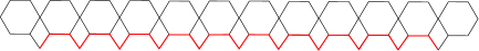
Figure 1. The transformations of $w^{2}$ to the word with reduced middle part $(1b23a4)^{3}$.

6.4 Corollary.

The word $w^{n}$ has form

$$w^{n}=1a3(1b23a4)^{2n-1}2b4$$

and, hence, it has length at least $12n-12$.

Proof.

Note that $w^{2}\cdot w$ reduces to

$$1a3\cdot 1b2\cdot 3a4\cdot 2b1\cdot 4a3\cdot 1b2\cdot 3a4\cdot 2b4\cdot a1ab3ba2ab4b\to$$

$$1a3\cdot 1b23a42b14a31b23a4\cdot 2b4\cdot 1a13b32a24b4\to$$

$$1a3\cdot 1b23a42b14a31b23a4\cdot 2b1\cdot 4a3\cdot 1b2\cdot 3a4\cdot 2b4\to 1a3\cdot(1b23a4)^{5}2b4.$$

In general, we see that $w^{n}$ reduces to

$$1a3\cdot 1b2\cdot 3a4\cdot 1b2\cdot 3a4\cdot 1b2\cdot 3a4\cdot 2b4\to 1a3(1b23a4)^{2n-1}2b4.$$

The estimate of the length comes from having $6(2n-1)+6$ letters. The part of length $6(2n-1)$ is reduced and we allow for cancellation of the prefix and suffix, with $3$ letters each, cancelling at most $12$ letters. ∎

6.5 Proposition.

The word $w^{n}=(a1ab3ba2ab4b)^{n}$ is reduced for all $n\geq 2$.

Proof.

We assume it is not, then there is a power $p$ of $w$ such that $w^{p}$ is not reduced. The word $w^{p}$ has $12p$ letters. Denote by $w^{p}_{-}$ and $w^{p}_{+}$ the beginning and end of the path in the Cayley graph labelled by $w^{p}$. We assume first, there is a shorter connection between $w^{p}_{-}$ and $w^{p}_{+}$ in the Cayley graph with at most $12p-1$ letters. Now assume $n\geq 13\cdot p$ and denote by $w^{n}_{-}$ and $w^{n}_{+}$ the beginning and end of the path in the Cayley graph labelled by $w^{n}$. This is depicted in Figure (2).

length $12n-6$ at 150 -5 $12p-1$ at 27 35 $12p-6$ at 40 15 $\dots\dots$ at 250 20

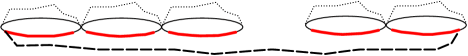
Figure 2. The word $w^{n}$, each block represents $w^{p}$ as in Figure 1 where the red line represents the reduced part.

There are $n/p$ copies of $w^{p}$ connecting $w^{n}_{-}$ with $w^{n}_{+}$. Denote by $s_{-}$ and $s_{+}$ the two vertices connecting the reduced middle part $(1b23a4)^{2n-1}$ of length $12n-6$ of $w^{n}$. Because each part $w^{p}$ of $w^{n}$ is connected by a path of length $12p-1$, we get a connection from $s_{-}$ to $s_{+}$ of length at most

$$\tfrac{n}{p}\cdot(12p-1)+6=12n-\tfrac{n}{p}+6\leq 12n-13+6=12n-7.$$

However, by Corollary 6.2 the subword $(1b23a4)^{2n-1}$ between $s_{-}$ and $s_{+}$ has length $12n-6$. ∎

6.6 Theorem.

The word $w^{n}=(a1ab3ba2ab4b)^{n}$ is a u.l.g.

Proof.

We observe that asymptotically there are each one third $a$’s, one third $b$’s and $\frac{1}{12}th$ every number $1,2,3$ and $4$. We first show that the only way to have a u.l.g. with this distribution is a periodic word. Assume the infinite word is not periodic. Then the maximal distance between two occurances of one of the letters $1,2,3,4$ must be bigger than $12$, because it is $12$ on average. Assume without loss of generality that it is the letter $1$ which has two occurances in the infinite word of distance more than $12$. Because of the symmetries of the Coxeter tree defining $\tilde{D}_{6}$ the same arguments work for $2,3$ and $4$. This can only happen in one of the following cases. (Recall that a u.l.g. has to be a connected path in the graph.)

We go through all other possiblities which do not yield the word $(a1ab3ba2ab4b)^{n}$. Most of them either contain either $xyxy$, $xyx\dots xyx$ or $xy\dots yxy$ with no $x$ in the dots. The first two are not reduced words, the latter not a u.l.g. A complete list of cases can be found in the Appendix 7.2. We discuss only the cases which are not immediate:

1. $a1a2ab4b$

2. $a1ab4ba2ab3ba1$

3. $a1ab4b3ba2ab4ba1a$

4. $a1ab4b3bab4b3b$

5. $a1ab4ba2ab3b4bab3b$

6. $a1ab4ba2ab3b4ba1a$

7. $a1ab4ba2ab3b4ba1ab3b$

8. $a1ab4ba2ab3b4ba1a2ab3b$

9. $a1ab4ba2ab3b4ba1a2aba1a2a$

10. $a1ab4b3ba2ab4b3ba1a2ab4b$

11. $a1ab4b3ba2ab4b3ba1a2aba1a$

12. $a1ab4b3ba2ab4b3ba1a2abab$

13. $a1ab4b3ba2ab4b3ba1ab4b$

(5) Isomorphic to (6) and follows because of the isomorphism $3\leftrightarrow 4$.

(17) $a1ab4ba2ab3ba1$ in this case the letter $1$ occurs with distance $12$.

(23) $a1ab4b3ba2ab4ba1a$ this is the complex case: We easily verify that neither $b4b$, $b3b$ nor $ab$ can be a prefix. Hence the only case to check is $a2a1a\dots$:

This can only occur after $aba2a1a\dots$, which can only occur after either

$$a1\cdot aba2a1a\dots\mbox{ or }a2\cdot aba2a1a\dots.$$

The word $a2aba2a1a=2a2\cdot ba2a1a=2ab\cdot 2a2a\cdot 1a$ is not reduced. Hence we need to check $a1aba2a\cdot a1a\dots$:

$$a1aba2a1ab4b3ba2ab4ba1a=\; a1ab\cdot 2a2\cdot 1ab4b3ba2ab4ba1a$$

$$a1ab\cdot 2a1\cdot 2a\cdot b4b3ba2ab4ba1a=\; a1ab\cdot 2a1\cdot a2a2\cdot b4b3ba2ab4ba1a$$

$$a1ab2a1a2ab4b3b\cdot 2a2a\cdot b4ba1a=\; 1a1\cdot b2a1a2ab4b3ba2b4ba1a$$

$$1a\cdot b2\cdot 1a1a\cdot 2ab4b3ba2b4ba1a=\; 1ab2\cdot a1\cdot 2ab4b3ba2b4ba1a.$$

The first word has length $23$ the last word has length $21$, hence it is not reduced and cannot occur as part of a u.l.g.

(27)

$$a1ab4b3bab4b3b=a1ab4b3\cdot aba\cdot 4b3b=\; a1a\cdot 4b4\cdot 3aba4b3b$$

$$a1a4b3a\cdot 4b4\cdot ab3b=\; a1a4b3a\cdot b4b\cdot ab3b$$

$$a14aba3\cdot b4b\cdot ab3b=\; a14\cdot bab\cdot 3b4bab3b.$$

Both the first and last term have $3$ times $a$, six times $b$, once $1$ and twice each $3$ and $4$. Hence it cannot be part of a u.l.g.

(28) This word is not reduced:

$$a1ab4ba2ab3b4bab3b=\; a1ab4ba2a\cdot 3b3\cdot 4bab3b$$

$$a1ab4ba2a\cdot 3b\cdot 4\cdot 3b\cdot ab3b=\; a1ab4ba2a\cdot b3b3\cdot 4\cdot 3b\cdot ab3b$$

$$a1ab4ba2a\cdot 3b4\cdot b3b3\cdot ab3b=\; a1ab4ba2a\cdot 3b4\cdot b3b\cdot a\cdot 3b3b$$

$$a1ab4ba2a\cdot 3b4b3b\cdot a\cdot b3=\; a1ab4ba2a3\cdot 4b4\cdot 3bab3$$

$$=\; a1a\cdot b4b4\cdot a2a3b43bab3.$$

(31) This is the inverse of 23. Hence it cannot be succeeded by anything valid.

(33) This word is not reduced:

$$a1ab4ba2ab3b4ba1ab3b=\; a1ab4ba2a\cdot 3b3\cdot 4ba1ab3b$$

$$a1ab4ba2a3b\cdot 4\cdot b3b3\cdot a1ab3b=\; a1ab4ba2a3b4\cdot b3b\cdot a1a\cdot 3b3b$$

$$a1ab4ba2a3\cdot 4b4\cdot 3ba1a\cdot b3=\; a1ab4b4\cdot a2a3\cdot b4\cdot 3ba1ab3$$

$$=\; a1a\cdot 4b\cdot a2a3b43ba1ab3.$$

(36) This word is not reduced:

$$a1ab4ba2ab3b4ba1a2ab3b=\; a1ab4ba2a\cdot 3b3\cdot 4ba1a2ab3b$$

$$a1ab4ba2a\cdot 3b4\cdot b3b3\cdot a1a2ab3b=\; a1ab4ba2a\cdot 3\cdot 4b4\cdot 3ba1a2a\cdot b3$$

$$a1a\cdot b4b4\cdot a2a34b43ba1a2ab3=\; a1a\cdot 4b\cdot a2a34b43ba1a2ab3.$$

(52) We study the end of the sequence $a2ab3b4ba1a2aba1a2a$ and show it is not reduced:

$$a2ab3b4ba1a2aba1a2a=\; a2ab3b4ba1\cdot 2a2\cdot ba1a2a$$

$$a2ab3b4ba\cdot 21\cdot a2ba1a2a=\; a2ab3b4b\cdot 2a2a\cdot 1a2b\cdot 1a1\cdot 2a$$

$$a2a\cdot 2\cdot b3b4ba2\cdot 1a1\cdot 2b\cdot 1a1\cdot 2a=\; 2a\cdot b3b4ba2\cdot 1a\cdot 2b\cdot a1\cdot 2a.$$

(59) This word is not reduced:

$$a1ab4b3ba2ab4b3ba1a2ab4b=\; a1ab4b3ba2ab4\cdot 3b3\cdot a1a2ab4b$$

$$a1ab4b3ba2a\cdot 3b3b\cdot 4b3a1a2ab4b=\; a1ab4\cdot 3b\cdot a2ab3\cdot 4b4\cdot 3a1a2ab4b$$

$$a1ab43ba2ab34b\cdot 3a1a2a\cdot 4b4b.$$

(60) This word is not reduced:

$$a1ab4b3ba2ab4b3ba1a2aba1a=\; a1ab4b3ba2ab4b3ba1\cdot 2a2\cdot ba1a$$

$$a1ab4b3ba2ab4b3b\cdot 2a2a\cdot 1\cdot a2\cdot ba1a=\; a1ab4b3b\cdot a2a2\cdot b4b3ba2a1a2ba1a$$

$$a1ab4b3b\cdot 2a\cdot b4b3ba2\cdot 1a1\cdot 2ba1a=\; a1ab4b3b2ab4b3ba21a2b\cdot 1a1a.$$

(62) The same as in 59, since the extra $a1a2$ in (59) has no effect on the technique.

(68) $a1ab4b3ba2ab4b3ba1ab4b$ is not reduced by the same argument as in (59) as well.

It is left to show that the above word does not transform into the one under the isomorphisms $3\mapsto 4$ or $1\mapsto 2$.

Case 1: We look at $3\mapsto 4$ first:

$$w^{2}=\; a1ab3ba2ab4ba1ab3ba2ab4b=1a1\cdot 3b3\cdot 2a2\cdot 4b4\cdot 1a1\cdot 3b3\cdot 2a2\cdot 4b4$$

$$=\; 1a31b23a42b14a31b23a42b4=1a32b13a41b23a42b13a42b4$$

$$=\; 1a32b31a14b42a23b31a24b4=1a23b3a1ab4ba2ab3b1a24b4.$$

Even though the last transformation of $w^{2}$ contains the word $w_{2}=a1ab4ba2ab3b$, the letter $1$ occurs more often than in $w^{2}$. Further, the last line is not a u.l.g. which implies that $w^{n}$ is a u.l.g.

Case 2: We now check the isomorphism $1\mapsto 2$.

$$w^{2}= \;a1ab3ba2ab4b\cdot a1ab3ba2ab4b=1a1\cdot 3b3\cdot 2a2\cdot 4b4\cdot 1a1\cdot 3b3\cdot 2a2\cdot 4b4$$

$$= \;1a31b23a42b14a31b23a42b4=1a3\cdot 2b1\cdot 3a4\cdot 1b2\cdot 3a4\cdot 2b1\cdot 3a42b4$$

$$= \;1a3\cdot b41\cdot 2a2\cdot 3b3\cdot 1a1\cdot 4b4\cdot 2a2\cdot 3b4=1a3b41\cdot a2ab3ba1ab4b\cdot 2a23b4.\qed$$

6.7 Corollary.

The words $w_{2}^{n}=(a1ab4ba2ab3b)^{n}$ and $w_{3}^{n}=(a2ab3ba1ab4b)^{n}$ are u.l.g.’s for all $n\geq 1$.

We finish with an observation regarding the two bi-infinite geodesic rays of $w^{n}$ and $w_{2}^{n}$ in the Cayley graph of $W$. We say two geodesics $\gamma_{1}$ and $\gamma_{2}$ are fellow travelling if there exists a constant $D$ such that every point on $\gamma_{2}$ is at distance at most $D$ from a point on $\gamma_{1}$.

6.8 Theorem.

The bi-infinite u.l.g.’s with labels

1. $w^{n}=(a1ab3ba2ab4b)^{n}$

2. $w_{2}^{n}=(a1ab4ba2ab3b)^{n}$

3. and $w_{3}^{n}=(a2ab3ba1ab4b)^{n}$

are fellow travelling at distance at most $5$ but at least $2$ from each other on their entire lengths.

$a$ at 30 160 $1$ at 55 175 $a$ at 87 165 $b$ at 99 165 $3$ at 130 175 $b$ at 152 165 $a$ at 165 165 $2$ at 190 175 $a$ at 218 165 $b$ at 228 165 $4$ at 260 175 $b$ at 282 165 $a$ at 295 165 $1$ at 320 175 $a$ at 346 165 $b$ at 358 162 $3$ at 380 175 $b$ at 412 165 $a$ at 422 165 $2$ at 450 175 $a$ at 475 165 $b$ at 490 165 $4$ at 510 175 $b$ at 540 165 $a$ at 553 160 $1$ at 580 175 $a$ at 605 165 $b$ at 618 165 $3$ at 640 175 $b$ at 670 165 $a$ at 682 165 $2$ at 705 175 $a$ at 735 165 $b$ at 748 165 $4$ at 775 175 $b$ at 803 165

$a$ at 30 15 $1$ at 55 -5 $a$ at 87 10 $b$ at 100 10 $4$ at 130 -5 $b$ at 152 10 $a$ at 163 12 $2$ at 190 -5 $a$ at 215 10 $b$ at 226 10 $3$ at 260 -5 $b$ at 280 10 $a$ at 292 10 $1$ at 320 -5 $a$ at 345 10 $b$ at 358 10 $4$ at 380 -5 $b$ at 411 10 $a$ at 420 10 $2$ at 450 -5 $a$ at 477 10 $b$ at 488 10 $3$ at 510 -5 $b$ at 542 10 $a$ at 553 10 $1$ at 580 -5 $a$ at 607 10 $b$ at 618 10 $4$ at 640 -5 $b$ at 671 10 $a$ at 682 10 $2$ at 705 -5 $a$ at 736 10 $b$ at 749 10 $3$ at 775 -5 $b$ at 802 10

$1$ at 30 130 $a$ at 55 122 $1$ at 85 130 $4$ at 100 130 $b$ at 130 122 $4$ at 1300 130 $2$ at 165 130 $a$ at 190 122 $2$ at 2130 130 $3$ at 226 130 $b$ at 260 122 $3$ at 280 130 $1$ at 295 130 $a$ at 320 122 $1$ at 345 130 $4$ at 358 130 $b$ at 380 122 $4$ at 410 130 $2$ at 420 130 $a$ at 450 122 $2$ at 475 130 $3$ at 490 130 $b$ at 510 122 $3$ at 540 130 $1$ at 555 130 $a$ at 580 122 $1$ at 605 130 $4$ at 618 130 $b$ at 640 122 $4$ at 670 130 $2$ at 682 130 $a$ at 705 122 $2$ at 735 130 $3$ at 750 130 $b$ at 775 122 $3$ at 800 130

$3$ at 30 70 $a$ at 55 52 $4$ at 85 70 $2$ at 100 70 $b$ at 130 52 $1$ at 150 70 $3$ at 165 70 $a$ at 190 52 $4$ at 213 70 $2$ at 226 70 $b$ at 260 52 $1$ at 280 70 $3$ at 295 70 $a$ at 320 52 $4$ at 345 70 $2$ at 358 70 $b$ at 380 52 $1$ at 410 70 $3$ at 420 70 $a$ at 450 52 $4$ at 475 70 $2$ at 490 70 $b$ at 510 52 $1$ at 540 70 $3$ at 555 70 $a$ at 580 52 $4$ at 605 70 $2$ at 618 70 $b$ at 640 52 $1$ at 670 70 $3$ at 682 70 $a$ at 705 52 $4$ at 735 70 $2$ at 750 70 $b$ at 775 52 $1$ at 800 70

$3$ at 30 110 $4$ at 85 110 $1$ at 100 110 $2$ at 150 110 $3$ at 165 110

$4$ at 213 110 $2$ at 226 110

$1$ at 280 110 $3$ at 295 110

$4$ at 345 110 $2$ at 358 110

$1$ at 410 110 $3$ at 420 110

$4$ at 475 110 $2$ at 490 110

$1$ at 540 110 $3$ at 555 110

$4$ at 605 110 $2$ at 618 110

$1$ at 670 110 $3$ at 682 110

$4$ at 735 110 $2$ at 750 110

$1$ at 800 110

Figure 3. The geodesic $w^{n}$ on the top, the geodesic $w_{2}^{n}$ on the bottom.

Proof.

We can reduce $w^{2}=a1ab3ba2ab4b\cdot a1ab3ba2ab4b$ as follows:

$$w^{2}=\; 1a1\cdot 3b3\cdot 2a2\cdot 4b4\cdot 1a1\cdot 3b3\cdot 2a2\cdot 4b4$$

$$=\; 1a31b23a42b14a31b23a42b4=1a32b13a41b23a42b13a42b4$$

$$=\; 1a32b31a14b42a23b31a24b4=1a23b3a1ab4ba2ab3b1a24b4.$$

We note that a cyclic permutation of the last line gives $w_{2}^{2}$ and we applied $6$ relations to get to the last line. However, as it can be verified in Figure 3, the shortest distance actually remains uniformly bounded above by $5$.

We note that this method is independent of how many copies of $w$ we had in the beginning. In a similar fashion it can be seen that we can obtain $w_{3}=a2ab3ba1ab4b$. Hence we have a bundle of three bi-infinite geodesics which remain at distance at most $5$ from each other. ∎

7. Appendix

7.1. Type $A$ examples

We list the u.l.g.’s with different labels for the groups of type $A_{n}$ for $n=3,4,5$ by enumerating all total labels which give a u.l.g. including the word of length $0$, which gives the constant term in the generating function. It can be verified that these numbers correspond to the formula in Corollary 3.7.

Type	Labels of u.l.g.’s	Total
		number
$A_{3}$	100 110 120 122 010 011 012 221 001 111 021 131 121	15
	210 000
$A_{4}$	Type I: 1000 0100 0010 0001 1100 0110 0011 0111 1110	33
	1111 0000
	Type II and III: 1200 0120 0012 1210 0121 1220 0122
	0021 2210 0221 2221 1321 1231 1331 1310 0131 1211 1121
	1222 1221 0210 2100
$A_{5}$	Type I: 10000 01000 00100 00010 00001 11000 01100 00110	66
	00011 11100 01110 00111 11110 01111 11111 00000
	Type II: 12000 01200 00120 00012 21000 02100 00210 00021
	01220 00122 22100 02210 00221 12220 01222 22210 02221
	22221 12100 01210 00121 12110 01211 11210 01121 12111
	12210 01221 12211 11221 12221 12200 12222 11121
	Type III: 12121 12321 12310 13210 13100 01310 00131
	01231 12331 13321 12231 13221 13310 01331 13331 01321

7.2. Infinite u.l.g.’s in the group $\tilde{D}_{6}$

We list all cases that have to be considered in Theorem 6.6. Figure 4 depicts the first part of these words, and the corresponding end-vertices of the trees labelled with $T2$, $T3$ and $T4$ indicate that the tree continues with Figure 5, 6 or 7.

1. $a1a2a1a$

2. $a1a2a2$

3. $a1a2aba2a$

4. $a1a2abab$

5. $a1a2ab4b$

6. $a1a2ab3b3b$

7. $a1a2ab3b4ba2a$

8. $a1a2ab3b4b3b$

9. $a1a2ab3bab$

10. $a1a2ab3ba2a$

11. $a1aba2ab$

12. $a1aba2a2$

13. $a1ab3bab$

14. $a1ab3b4b$

15. $a1ab4bab$

16. $a1ab4ba2ab4b$

17. $a1ab4ba2ab3ba1$

18. $a1ab4b3b4b$

19. $a1ab4b3ba2aba$

20. $a1ab4b3ba2ab3b$

21. $a1ab4b3ba2ab4b3b3$

22. $a1ab4b3ba2ab4ba2a$

23. $a1ab4b3ba2ab4ba1a$

24. $a1ab4b3baba$

25. $a1ab4b3bab3b$

26. $a1ab4b3bab4ba$

27. $a1ab4b3bab4b3b$

28. $a1ab4ba2ab3b4bab3b$

29. $a1ab4ba2ab3b4bab4b$

30. $a1ab4ba2ab3b4baba$

31. $a1ab4ba2ab3b4ba1a$

32. $a1ab4ba2ab3b4ba2a$

33. $a1ab4ba2ab3b4ba1ab3b$

34. $a1ab4ba2ab3b4ba1ab4b$

35. $a1ab4ba2ab3b4ba1aba$

36. $a1ab4ba2ab3b4ba1a2ab3b$

37. $a1ab4ba2ab3b4ba1a2ab4b$

38. $a1ab4ba2ab3b4ba1a1$

39. $a1ab4ba2ab3b4b3b$

40. $a1ab4ba2ab3b4b4$

41. $a1ab4b4$

42. $a1ab4b3b3$

43. $a1ab4b3ba2a2$

44. $a1ab4b3bab4b4$

45. $a1ab4ba2a2$

46. $a1ab4ba2ab3b3$

47. $a1ab4b3ba2ab4b4$

48. $a1ab4b3ba2ab4bab$

49. $a1ab4ba2ab3b4ba1a2abab$

50. $a1ab4ba2ab3b4ba1a2aba2a$

51. $a1ab4ba2ab3b4ba1a2aba1ab$

52. $a1ab4ba2ab3b4ba1a2aba1a2a$

53. $a1ab4ba2ab3b4ba1a2aba1a1a$

54. $a1ab4b3ba2ab4b3b4b$

55. $a1ab4b3ba2ab4b3ba2a$

56. $a1ab4b3ba2ab4b3ba1aba$

57. $a1ab4b3ba2ab4b3ba1a1a$

58. $a1ab4b3ba2ab4b3ba1a2ab3b$

59. $a1ab4b3ba2ab4b3ba1a2ab4b$

60. $a1ab4b3ba2ab4b3ba1a2aba1a$

61. $a1ab4b3ba2ab4b3ba1a2aba2a$

62. $a1ab4b3ba2ab4b3ba1a2abab$

63. $a1ab4b3ba2ab4b3baba$

64. $a1ab4b3ba2ab4b3bab4b$

65. $a1ab4b3ba2ab4b3bab3b$

66. $a1ab4ba2aba$

67. $a1ab4b3ba2ab4b3ba1ab3b$

68. $a1ab4b3ba2ab4b3ba1ab4b$

Checking the cases of the tree:

• The following cases have been shown in the proof of Theorem 6.6:

  $$\small{\{\eqref{cases:5},\eqref{cases:19},\eqref{cases:30},\eqref{cases:33},\eqref{cases:35},\eqref{cases:38},\eqref{cases:54},\eqref{cases:61},\eqref{cases:62},\eqref{cases:64},\eqref{cases:70}\}.}$$

• The following cases contain a sequence $xyxy$ and are hence not reduced:

  $${\small\{\ref{cases:2},\ref{cases:4},\ref{cases:6},\ref{cases:12},\ref{cases:23},\ref{cases:26},\ref{cases:32},\ref{cases:40},\ref{cases:42},\ref{cases:43},\ref{cases:44},\ref{cases:45},\ref{cases:46},\ref{cases:47},\ref{cases:48},\ref{cases:49},\ref{cases:51},\ref{cases:55},\ref{cases:64},\ref{cases:65}\}.}$$

• The following cases contain $xyx\dots xyx$ where the dots do not contain $x$ or $y$. These cases are not reduced:

  $${\small\{\ref{cases:1},\ref{cases:3},\ref{cases:7},\ref{cases:8},\ref{cases:10},\ref{cases:18},\ref{cases:20},\ref{cases:22},\ref{cases:24},\ref{cases:27},\ref{cases:31},\ref{cases:34},\ref{cases:36},\ref{cases:41},\ref{cases:52},\ref{cases:56},\ref{cases:57},\ref{cases:59},\ref{cases:60},\ref{cases:63},\ref{cases:67},\ref{cases:69}\}.}$$

• The following cases contain $xy\dots yxy$ and are hence not a u.l.g.:

  $${\small\{\ref{cases:9},\ref{cases:11},\ref{cases:15},\ref{cases:17},\ref{cases:21},\ref{cases:28},\ref{cases:37},\ref{cases:39},\ref{cases:50},\ref{cases:53},\ref{cases:58},\ref{cases:68}\}.}$$

$1$ at 150 280 $a$ at 150 260 $b$ at 140 250 $3$ at 120 240 $b$ at 80 210 $4$ at 50 200 $b$ at 20 180 $a$ at 60 180 $b$ at 55 170 $4$ at 120 220 $a$ at 145 220 $2$ at 135 180 $a$ at 120 160 $b$ at 90 130 $2$ at 120 130 $2$ at 180 240 $a$ at 210 200 $b$ at 250 190 $1$ at 215 180 $a$ at 205 160 $2$ at 240 170 $3$ at 300 170 $a$ at 260 150 $b$ at 250 120 $2$ at 290 110 $a$ at 280 80 $4$ at 300 150 $b$ at 320 110 $b$ at 360 150 $3$ at 350 120 $4$ at 370 120 $b$ at 370 90 $a$ at 360 60 $2$ at 350 40 $a$ at 330 20 $b$ at 380 60 $3$ at 405 40 $b$ at 395 10 $a$ at 380 130 $2$ at 420 110 $b$ at 400 90 $a$ at 440 80

at 0 157 at 40 150 at 103 200 at 70 110 at 120 110 at 200 135 at 235 152 at 260 80 at 290 47 at 310 80 at 350 100 at 320 0 at 412 0 at 409 75 at 440 45

Figure 4. Tree 1

$a$ at 150 370 $4$ at 200 380 $b$ at 90 330 $2$ at 120 330 $b$ at 180 330 $a$ at 90 290 $b$ at 60 250 $2$ at 90 250 $a$ at 20 230 $4$ at 30 210 $3$ at 60 210 $b$ at 50 180 $a$ at 40 150 $4$ at 70 140 $1$ at 20 120 $a$ at 0 70 $b$ at 70 100 $3$ at 40 60 $a$ at 50 50 $4$ at 80 50 $3$ at 180 370 $a$ at 230 290 $3$ at 180 280 $4$ at 210 280 $b$ at 200 250 $b$ at 280 270 $2$ at 260 250 $a$ at 260 220 $b$ at 260 180 $4$ at 220 150 $b$ at 180 120 $4$ at 150 80 $3$ at 160 70 $b$ at 160 40 $a$ at 190 90 $1$ at 220 70 $a$ at 270 30 $2$ at 210 50 $a$ at 210 30 $a$ at 230 130 $3$ at 260 130 $b$ at 290 100 $a$ at 290 230 $3$ at 320 230 $4$ at 330 250 $b$ at 340 200 $b$ at 370 210 $a$ at 370 180 $3$ at 410 180 $b$ at 440 165

at 0 220 at -5 180 at 63 300 at 100 208 at -7 50 at 20 30 at 63 23 at 110 23 at 170 260 at 205 215 at 235 105 at 130 50 at 160 10 at 200 0 at 260 -8 at 300 80 at 305 190 at 345 170 at 380 155 at 440 145 at 260 367

Figure 5. Tree 2

$b$ at 80 300 $4$ at 60 280 $b$ at 50 270 $3$ at 60 260 $a$ at 85 260 $b$ at 75 250 $a$ at 60 230 $1$ at 90 240 $a$ at 85 220 $1$ at 140 300 $2$ at 100 270 $a$ at 110 240 $a$ at 200 260 $2$ at 240 240 $1$ at 180 230 $b$ at 215 230 $a$ at 180 210 $3$ at 200 190 $4$ at 220 190 $b$ at 200 160 $b$ at 235 160 $a$ at 260 210 $b$ at 300 190 $a$ at 260 140 $3$ at 300 150 $4$ at 330 160 $b$ at 280 120 $b$ at 340 130 $2$ at 190 100 $a$ at 150 80 $1$ at 220 100 $b$ at 250 100 $a$ at 210 70 $b$ at 180 50 $2$ at 200 40 $a$ at 200 20 $1$ at 230 50 $a$ at 255 20

at 0 225 at 25 220 at 50 195 at 90 195 at 110 210 at 162 215 at 145 190 at 185 120 at 225 135 at 115 50 at 170 23 at 195 0 at 268 0 at 270 75 at 280 105 at 340 105

Figure 6. Tree 3

$3$ at 100 300 $b$ at 50 270 $b$ at 80 270 $4$ at 140 300 $a$ at 170 300 $b$ at 140 240 $3$ at 110 210 $b$ at 80 170 $4$ at 125 200 $a$ at 150 200 $2$ at 180 240 $a$ at 175 200 $1$ at 200 250 $a$ at 240 200 $b$ at 220 180 $a$ at 190 150 $3$ at 210 150 $4$ at 230 150 $b$ at 180 110 $b$ at 220 110 $1$ at 237 170 $2$ at 260 170 $a$ at 280 140 $b$ at 300 100 $a$ at 320 80 $4$ at 290 80 $3$ at 305 70 $b$ at 270 60 $b$ at 290 60 $1$ at 320 50 $a$ at 320 20 $b$ at 350 60 $2$ at 340 40 $a$ at 340 10

at 0 235 at 40 235 at 70 148 at 122 145 at 150 180 at 175 180 at 170 130 at 170 90 at 220 90 at 245 145 at 260 33 at 290 30 at 305 0 at 355 0 at 375 33

Figure 7. Tree 4

References

- [AC13] Y. Antolin, L. Ciobanu, Geodesic growth in right-angled and even Coxeter groups, European Journal of Combinatorics 34 (2013), 859–874.
- [A04] A. Avasjö, Automata and growth functions of Coxeter groups, Licentiate Thesis Department of Mathematics, KTH, 2004.
- [BB] A. Björner, F. Brenti, Combinatorics of Coxeter Groups, GTM 231, Springer, 2005.
- [BH93] B. Brink and R. Howlett, A finiteness property and an automatic structure for Coxeter groups, Math. Ann. 296, (1993), 179–190.
- [CD91] R. Charney, M. Davis, Reciprocity of growth functions of Coxeter groups, Geometriae Dedicata 39 (1991), Issue 3, 373–378.
- [CK16] L. Ciobanu, A. Kolpakov, Geodesic growth of right-angled Coxeter groups based on trees, J. Algebr. Comb. 44 (2016), 249–264.
- [Ed95] P. Edelman, Lexicographically first reduced words, Discrete Math. 147 (1995), no.1-3, 95–106.
- [El97] S. Elnitsky, Rhombic tilings of polygons and classes of reduced words in Coxeter groups, J. Combin. Theory Ser. A 77 (1997), no. 2, 193 221.
- [EE10] H. Eriksson, K. Eriksson, Words with intervening neighbours in infinite Coxeter groups are reduced, The Electronic Journal of Combinatorics 17 (2010), no 9.
- [FZ07] S. Fomin, A. Zelevinsky, Cluster algebras. IV. Coefficients, Compositio Math. 143 (2007), no. 1, 112–164.
- [GN97] R. I. Grigorchuk, T. Nagnibeda, Complete growth functions of hyperbolic groups, Invent. Math. 130 (1997), 159–188.
- [Ha17] S. Hart, How many elements of a Coxeter group have a unique reduced expression? Preprint arXiv:1701.01138 (2017).
- [He94] P. Headley, Reduced expressions in infinite Coxeter groups, PhD Thesis, University of Michigan, 1994.
- [HNW] C. Hohlweg, P. Nadeau and N. Williams, Automata, reduced words, and Garside shadows in Coxeter groups, Journal of Algebra 457 (2016), 331–456.
- [Hu90] J. Humphreys, Reflection groups and Coxeter groups. Cambridge studies in Advanced Math. 29, Cambridge Univ. Press, 1990.
- [LP13] T. Lam, P. Pylyavskyy, Total positivity for loop groups II: Chevalley generators, Transformation Groups 18 (2013), no. 1, 179–231.
- [M03] M. J. Mamaghani, Complete growth series of Coxeter Groups with more than three generators, Bulletin of the Iranian Mathematical Society Vol. 29 No. 1 (2003), 65–76.
- [MT13] M. Mihalik, S. Tschantz, Geodesically tracking quasi-geodesic paths for Coxeter groups, Bull. London Math. Soc. 45 (2013), 700–714.
- [P90] L. Paris, Growth series of Coxeter groups, Group theory from a geometrical viewpoint (Trieste, 1990), 302–310, World Sci. Publ., River Edge, NJ, 1991.
- [S09] D. Speyer, Powers of Coxeter elements in infinite groups are reduced, Proceedings of the American Math. Soc. 137 (2009), no. 4, 1295–1302.
- [St84] R. Stanley, On the number of Reduced Decompositions of Elements of Coxeter groups, Europ. J. Combinatorics 5 (1984), 359–372.
- [St97] J. Stembridge, Some combinatorial aspects of reduced words in finite Coxeter groups, Transactions of the American Math. Soc. 349 (1997), no. 4, 1285–1332.