NOMA Assisted Wireless Caching:
Strategies and Performance Analysis

Abstract

Conventional wireless caching assumes that content can be pushed to local caching infrastructure during off-peak hours in an error-free manner; however, this assumption is not applicable if local caches need to be frequently updated via wireless transmission. This paper investigates a new approach to wireless caching for the case when cache content has to be updated during on-peak hours. Two non-orthogonal multiple access (NOMA) assisted caching strategies are developed, namely the push-then-deliver strategy and the push-and-deliver strategy. In the push-then-deliver strategy, the NOMA principle is applied to push more content files to the content servers during a short time interval reserved for content pushing in on-peak hours and to provide more connectivity for content delivery, compared to the conventional orthogonal multiple access (OMA) strategy. The push-and-deliver strategy is motivated by the fact that some users’ requests cannot be accommodated locally and the base station has to serve them directly. These events during the content delivery phase are exploited as opportunities for content pushing, which further facilitates the frequent update of the files cached at the content servers. It is also shown that this strategy can be straightforwardly extended to device-to-device caching, and various analytical results are developed to illustrate the superiority of the proposed caching strategies compared to OMA based schemes.

I Introduction

Recently non-orthogonal multiple access (NOMA) has received significant attention as a key enabling technique for future wireless networks [2, 3, 4]. The key idea of NOMA is to encourage spectrum sharing among mobile nodes, which not only improves the spectral efficiency but also ensures that massive connectivity can be effectively supported. Practical concepts for implementing the NOMA principle for a single resource block, such as an orthogonal frequency division multiplexing (OFDM) subcarrier, include power domain NOMA and cognitive radio (CR) inspired NOMA [5, 6, 7], which provide different tradeoffs between throughput and fairness. When each user is allowed to occupy multiple subcarriers, dynamically grouping the users on different subcarriers is a challenging problem, and various multi-carrier NOMA schemes, such as sparse code multiple access (SCMA) and pattern division multiple access (PDMA) [8, 9], provide practical solutions for achieving different performance-complexity tradeoffs. Unlike single-carrier NOMA, in multi-carrier NOMA, a user’s message is spread over multiple resource blocks, which requires efficient encoding schemes, such as multi-dimensional coding, to be implemented at the transmitter and low-complexity decoding schemes, such as message passing algorithms, to be used at the receivers.

NOMA has been shown to be compatible with many other advanced communication concepts. For example, several features of millimeter-wave (mmWave) communications, such as highly directional transmission, and the mismatch between the users’ channel vectors and the commonly used finite resolution analog beamforming, facilitate the implementation of NOMA in mmWave networks [10, 11]. In addition, NOMA can further improve the spectral efficiency of multiple-input multiple-output (MIMO) systems. For example, MIMO-NOMA can efficiently exploit the spatial degrees of freedom of MIMO channels and, unlike single-input single-output (SISO) NOMA, is beneficial even if the users have similar channel conditions [12, 13, 14]. Furthermore, conventionally, when the users have a single antenna, cooperative transmission can be used to exploit spatial diversity but suffers from a reduced overall data rate, since relaying consumes extra bandwidth resources [15]. In this context, the application of NOMA can efficiently reduce the number of consumed bandwidth resource blocks, such as subcarriers and time slots, and hence improve the spectral efficiency of cooperative communications [16, 17, 18]. Furthermore, existing studies have also revealed a strong synergy between NOMA and CR networks, where the use of NOMA can significantly improve the connectivity for the users of the secondary network [19].

Wireless caching is another important enabling technique for future communication networks [20, 21], but little is known about the coexistence of NOMA and wireless caching. The key idea of wireless caching is to push the content in off-peak hours during the so-called content pushing phase close to the users before it is requested, and therefore, the users’ requests can be locally served during the so-called content delivery phase. In fact, asking a base station (BS) to serve the users’ requests directly is not preferable, not only because the maximal number of users that a BS can serve concurrently is small, but also because non-caching transmission schemes are severely constrained by the limited backhaul capacity of wireless networks. Most caching schemes can be grouped into one of two classes [21, 24]. The first class assumes the existence of a content caching infrastructure, such as content servers, small cell BSs, etc., [25, 26, 27]. When caching infrastructure (e.g., content servers) is available, the objective in the content pushing phase is to push the content files to the content servers in a timely and reliable manner, before the users request these files. During the phase of content delivery, an ideal situation is that all the users’ requests can be locally served, without communicating with the central controller of the network, e.g., the BS. The second class, also known as device-to-device (D2D) caching, assumes that there is no dedicated caching infrastructure, and relies on user cooperation [28, 29]. Particularly, during the content pushing phase, all users will proactively cache some content. During the content delivery phase, a user will communicate with its BS only if none of its neighbours can help the user locally, i.e., the user cannot find its requested file in the caches of its surrounding neighbours.

A fundamental assumption made in the existing caching literature is that, in the content pushing phase, content is pushed to the content servers in an error-free manner during off-peak hours. However, performing caching only during off-peak hours is not effective if the popularity of the content is rapidly changing or the files to be cached need to be frequently updated. Typical examples for this type of content include up-to-the-minute news, sports events requiring live updates, e-commerce promotion with frequent pricing changes, newly released music videos, etc. Similarly, assuming error-free content pushing may also be questionable in many practical communication scenarios. In practice, connecting the content servers wirelessly with the BS is preferable since the cost for setting up the network is reduced and the installation of cables is avoided. Furthermore, wireless networks facilitate D2D caching, since file sharing among users in wireless networks is straightforward, whereas realizing pairwise connections in wireline networks is more difficult. However, wireless transmission is prone to noise, distortion, and attenuation, which makes error-free transmission a very strong assumption in practice. The objective of this paper is to apply the NOMA principle to wireless caching and to develop NOMA assisted caching strategies which do not require the aforementioned assumptions. The contributions of the paper are summarized as follows:

• For the case where the content pushing and delivery phases are separated and limited bandwidth resources are periodically available for content pushing in on-peak hours, a NOMA-assisted push-then-deliver strategy is proposed. Particularly, during the content pushing phase, the BS will use the NOMA principle and push multiple files to the content servers simultaneously. A CR inspired NOMA power allocation policy is used to ensure that content files are delivered to their target content servers with the same outage probability as with conventional orthogonal multiple access (OMA) based transmission. However, by using NOMA, additional files can be pushed to the content servers simultaneously, which is important to efficiently use the limited resources reserved for content pushing and hence to improve the cache hit probability. During the content delivery phase, the use of NOMA not only improves the reliability of content delivery, but also ensures that more user requests can be served concurrently by a content server.

• The objective of the proposed push-and-deliver strategy is to provide additional bandwidth resources for content pushing. Unlike the push-then-deliver strategy, the push-and-deliver strategy seeks opportunities for content pushing during the content delivery phase. In particular, during the content delivery phase, the BS occasionally has to serve some users directly, since these users’ requested files cannot be found in the local content severs. Conventionally, this is a non-ideal situation which reduces the spectral efficiency. Nevertheless, this non-ideal situation is inevitable in practice and is expected to occur frequently, as the users’ requests cannot be perfectly predicted. In this paper, this non-ideal situation for content delivery is exploited as an opportunity for additional content pushing. In other words, the push-and-deliver strategy is particularly useful when the bandwidth resources reserved for content pushing are limited, but the files at the content servers need to be frequently updated. The proposed push-and-deliver strategy is also extended to D2D caching without caching infrastructure, where the caches at the D2D helpers can be refreshed while users are directly served by the base station. We note that the NOMA-multicasting scheme proposed in [30] can be viewed as a D2D special case of the proposed push-and-deliver strategy, if the multicasting phase in [30] is viewed as the content delivery phase. However, the impact of integrating content pushing and delivery on the cache hit probability was not investigated in [30].

• Analytical results for the cache hit probability, the transmission outage probability, and the D2D cache miss probability are derived in order to obtain a better understanding of the performance of the proposed caching strategies. Conventionally, the cache hit probability is mainly determined by the size of the caches of the content servers, instead of by transmission outages, since conventional content pushing is carried out during off-peak hours, which means that the amount of the pushed content is much larger than the size of the caches of the content servers. However, for the schemes proposed in this paper, the outage based cache hit probability is a more suitable metric for performance evaluation, as explained in the following. In particular, we assume that a short time interval is periodically reserved during on-peak hours for pushing new content to the content servers. The time interval reserved for content pushing has to be short in order to achieve high spectral efficiency and has to be shared by multiple content servers. Thus, the amount of content that can be pushed to the content servers may be much smaller than the size of the storage of the content servers. Considering the tremendous increase in storage capacity available with current technologies, this is a realistic assumption. For the considered caching scenario, the crucial issue is how to quickly push the content files to the content servers during the short time interval available for content pushing during on-peak hours. Therefore, the outage based cache hit probability is the relevant performance criterion. When caching infrastructure is available, the impact of NOMA on the content pushing phase is quantified by exploiting the joint probability density function (pdf) of the distances between the content servers and the BS, and closed-form expressions for the achieved cache hit probability are developed. The impact of NOMA on the content delivery phase is investigated by using the transmission outage probability as a performance criterion and modelling the locations of the users and the content servers as Poisson cluster processes (PCPs). Furthermore, the impact of NOMA on D2D caching is studied by modelling the effect of content pushing as a thinning Poisson point process and deriving the cache miss probability, i.e., the probability of the event that a user cannot find its requested file in the caches of its neighbours. The provided simulations verify the accuracy of the proposed analysis, and illustrate the effectiveness of the proposed NOMA based wireless caching schemes.

The remainder of the paper is organized as follows. In Section II, the considered system model, including the caching model and the spatial model, are introduced. In Section III, the NOMA-assisted push-then-deliver strategy is presented, and its impact on the content pushing and delivery phases is investigated. In Section IV, the proposed push-and-deliver strategy is developed by efficiently merging the content pushing and delivery phases, its impact on the cache hit probability is investigated, and its extension to D2D scenarios is discussed. Computer simulations are provided in Section V, and the paper is concluded in Section VI. The details of all proofs are collected in the appendix.

II System Model

Consider a two-tier heterogeneous communication scenario, where multiple users request cacheable content with the help of one BS and multiple content servers. The D2D scenario without caching infrastructure, e.g., content servers, will be described in Section IV.C. Assume that each user is associated with a single content server. If the file requested by a user can be found in the cache of its associated content server, this server will serve the user, which means that multiple content servers can communicate with their respective users concurrently and hence the spectral efficiency is high. However, if the file requested by a user cannot be found locally, the BS will serve the user directly, a situation which is not ideal for caching and should be avoided. The assumption that each user is associated with a single content server facilitates the use of PCP modelling, as discussed in the following subsection.

II-A Spatial Clustering Model

Assume that the BS is located in the origin of a two-dimensional Euclidean plane, denoted by $\mathbb{R}^{2}$. As shown in Fig. 1, there are multiple content servers. The locations of the content servers and the users are modelled as PCPs. In particular, assume that the locations of the content servers are denoted by $x_{i}$ and are modelled as a homogeneous Poisson point process (HPPP), denoted by $\Phi_{c}$, with density $\lambda_{c}$, i.e., $x_{i}\in\Phi_{c}$. For notational simplicity, the location of the BS is denoted by $x_{0}$.

Each content server is the parent node of a cluster covering a disk whose radius is denoted by $\mathcal{R}_{c}$. Denote the content server in cluster $i$ by $\text{CS}_{i}$. Without loss of generality, assume that there are $K$ users associated with $\text{CS}_{i}$, denoted by $\text{U}_{i,k}$. Note that users associated with the same content server are viewed as offspring nodes [31]. The offspring nodes are uniformly distributed in the disk associated with $\text{CS}_{i}$, and their locations are denoted by $y_{i,k}$. To simplify the notation, the locations of the cluster users are conditioned on the locations of their cluster heads (content severs). As such, the distance from a user to its content server is simply given by $||y_{i,k}||$, and the distance from user $\text{U}_{i,k}$ to content server $\text{CS}_{j}$ is denoted by $||y_{i,k}+x_{i}-x_{j}||$ [32, 33].

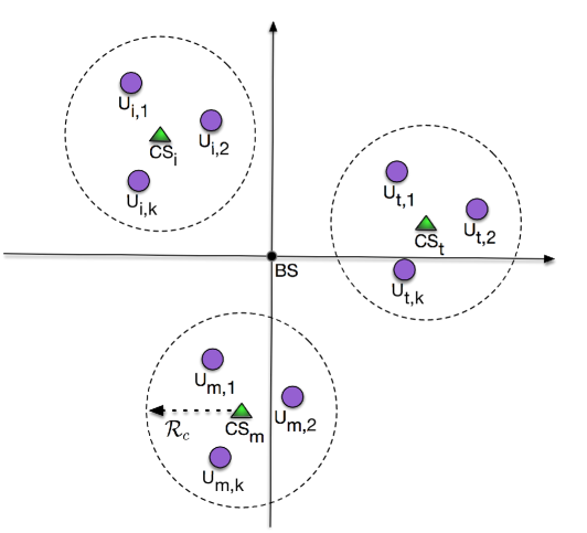
Figure 1: An illustration of the assumed spatial model.

II-B Caching Assumptions

Consider that the files to be requested by the users are collected in a finite content library $\mathcal{F}=\{f_{1},\cdots,f_{F}\}$. The popularity of the requested files is modelled by a Zipf distribution [34]. Particularly, the popularity of file $f_{i}$, denoted by $\mathrm{P}(f_{l})$, is modelled as follows:

$$\mathrm{P}(f_{l})=\frac{\frac{1}{l^{\gamma}}}{\sum^{F}_{p=1}\frac{1}{p^{\gamma}}},$$ (1)

where $\gamma>0$ denotes the shape parameter defining the content popularity skewness. We note that $\mathrm{P}(f_{l})$ is the probability that a user requests file $f_{i}$. Similar to the existing wireless caching literature, [20, 21, 25, 26, 27], packets belonging to different files are assumed to have the same length. However, unlike the existing literature, we do not assume that the amount of information contained in the packets of different files is identical. Particularly, the prefixed data rate of the packets of file $f_{l}$ is denoted by $R_{l}$. We assume that packets belonging to different files have the same size but may contain different amounts of information for the following reasons. Firstly, the packet size is typically predefined according to practical system standards and cannot be changed. Therefore, it is reasonable to assume that all packets have the same size. Secondly, packets belonging to different files have different priorities and different target reception reliabilities, which requires the use of different channel coding rates for different packets. As a result, packets which have the same size do not necessarily contain the same amount of information. We note that all analytical results developed in this paper, except for Lemma 2, do not require the assumption that the packets contain different amounts of information. In fact, the performance for the special case of identical target data rates for all files is investigated in the simulation section.

Finally, we assume that the BS has access to all files. In this paper, when content servers exist, we assume that the users have no caching capabilities. On the other hand, for the D2D assisted caching discussed in Section IV.C, it is assumed that each user has a cache.

III Push-then-deliver Strategy

In this section, we consider the case where the two caching phases, content pushing and content delivery, are separated. Unlike conventional caching which relies on the use of off-peak hours for content pushing, the proposed push-then-deliver strategy assumes that limited bandwidth resources, such as short time intervals, are periodically reserved for pushing new files to the content servers during on-peak hours. For example, every hour, a BS deployed in a large shopping mall or an airport may use a few seconds to push updated advertising and marketing videos to the content servers. The time interval reserved for content pushing during on-peak hours has to be short in order to achieve high system spectral efficiency. As will be shown, the proposed push-then-deliver strategy allows more files to be pushed within this short time interval compared to OMA.

In the following two subsections, we will demonstrate the impact of the NOMA principle on the content pushing and delivery phases, respectively.

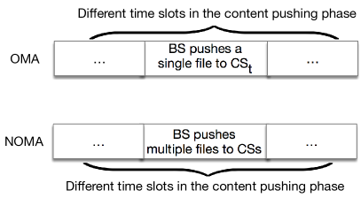
(a) A general illustration of the content pushing phase

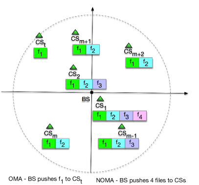
(b) An example for the outcome of content pushing

Figure 2: An illustration of the impact of NOMA on content pushing. “CS” denotes a content server in the subfigures. For the example shown in subfigure (b), it is assumed that $\text{CS}_{m}$ is closer to the BS than $\text{CS}_{t}$, for $1<m<t$. In OMA, a single file is pushed to $\text{CS}_{t}$, and in NOMA, the BS pushes a superimposed mixture consisting of four files, where content servers closer to the BS are likely able to decode more pushed files.

III-A Content Pushing Phase

In order to have a baseline for the performance of NOMA assisted content pushing, conventional OMA based content pushing is introduced first.

III-A1 OMA Based Content Pushing

In OMA, the BS divides the content pushing phase into multiple time slots, and different content servers are served during different time slots, as shown in Fig. 2(a). Without loss of generality, we focus on a time slot in which the BS needs to push a file to $\text{CS}_{t}$. Since the use of OMA means that only a single file can be pushed during this time slot, the BS will push the most popular file $f_{1}$ to $\text{CS}_{t}$ .

Therefore, $\text{CS}_{t}$ is able to decode file $f_{1}$ with the following achievable data rate:

$$R^{CP}_{t,OMA}=\log\left(1+\rho\frac{1}{{L\left(||x_{t}-x_{0}||\right)}}\right),$$ (2)

where $\rho$ denotes the transmit signal-to-noise ratio (SNR), and $\frac{1}{L\left(||x_{t}||\right)}$ is the large scale path loss between $\text{CS}_{t}$ and the BS located at $x_{0}$. Particularly, the following path loss model is used, $\frac{1}{L\left(||x_{t}||\right)}$, where $L\left(||x_{t}||\right)=||x_{t}||^{\alpha}$ and $\alpha$ denotes the path loss exponent. For a large scale network, the probability that $||x_{t}-x_{0}||<1$ is very small, and therefore, the simplified unbounded path loss model is used in this paper [35, 32, 33]. Nevertheless, the presented analytical results can be extended to other path loss models, e.g., $L\left(||x_{t}||\right)=||1+x_{t}||^{\alpha}$ or $L\left(||x_{t}||\right)=\max\{1,||x_{t}||^{\alpha}\}$, in a straightforward manner. We note that small scale multi-path fading is not considered for the channel gain associated with $\text{CS}_{t}$ since the content servers can be deployed such that line-of-sight connections to the BS are ensured, which means that large scale path loss is the dominant factor for signal attenuation. However, small scale fading will be considered for the channel gains associated with the users, since the users may not have line-of-sight connections to their transmitters.

III-A2 NOMA Assisted Content Pushing

By applying the concept of NOMA, more content can be simultaneously delivered from the BS to the content servers, as illustrated in Fig. 2(b). Particularly, the BS sends the following mixture, which contains the $M_{s}$ most popular files:

$$s_{i}=\sum^{M_{s}}_{i=1}\alpha_{i}\bar{f}_{i},$$ (3)

where $\bar{f}_{i}$ denotes the signal which represents the information contained in file $f_{i}$, $\alpha_{i}$ denotes the real-valued power allocation coefficient and $\sum^{M_{s}}_{i=1}\alpha_{i}^{2}=1$. The content servers carry out successive interference cancellation (SIC). The SIC decoding order is determined by the priority of the files, i.e., a more popular file, $f_{i}$, will be decoded before a less popular file, $f_{j}$, $i<j$. Suppose that the files $f_{j}$, $j<i$, have been decoded and subtracted correctly by content server $\text{CS}_{m}$. In this case, $\text{CS}_{m}$ can decode the next most popular file, $f_{i}$, with the following data rate:

$$R^{CP}_{m,i}= \log\left(1+\frac{\rho\alpha_{i}^{2}\frac{1}{{L\left(||x_{m}-x_{0}||\right)}}}{\rho\frac{1}{{L\left(||x_{m}-x_{0}||\right)}}\sum^{M_{s}}_{j=i+1}\alpha_{j}^{2}+1}\right).$$ (4)

If $R^{CP}_{m,i}\geq R_{i}$, then file $f_{i}$ can be decoded and subtracted correctly at $\text{CS}_{m}$.

For a fair comparison with OMA, which pushes only one file at a time, a sophisticated power allocation policy is needed for the NOMA scheme. Without loss of generality, we assume that the content servers are ordered as follows:

$$\frac{1}{{L\left(||x_{1}-x_{0}||\right)}}\cdots\geq\frac{1}{{L\left(||x_{m}-x_{0}||\right)}}\geq\cdots\geq\frac{1}{{L\left(||x_{t}-x_{0}||\right)}}\geq\cdots,$$ (5)

for $1\leq m<t$. Furthermore, since the considered time slot is used to push $f_{1}$ to $\text{CS}_{t}$, we make the following quality of service (QoS) assumption, in order to facilitate the design of the power allocation coefficients:

QoS Target: The most popular file, $$f_{1} t \text{CS}_{t}$$, needs to reach the -th nearest content server ().

Both the OMA and NOMA transmission schemes need to ensure this QoS target. Therefore, the CR inspired power allocation policy can be used for NOMA [7], i.e., power allocation coefficient $\alpha_{1}$ is chosen such that $f_{1}$ can be delivered reliably to $\text{CS}_{t}$, i.e.,

$$R^{CP}_{t,1}\geq R_{1}.$$ (6)

This constraint results in the following choice of $\alpha_{1}$:

$$\alpha_{1}^{2}=\min\left\{1,\frac{\epsilon_{1}\left(\rho\frac{1}{{L\left(||x_{t}-x_{0}||\right)}}+1\right)}{\rho(1+\epsilon_{1})\frac{1}{{L\left(||x_{t}-x_{0}||\right)}}}\right\},$$ (7)

where $\epsilon_{l}=2^{R_{l}}-1$. The use of the power allocation policy in (7) ensures that the outage probability for pushing file, $f_{1}$, to $\text{CS}_{t}$ is the same as that for OMA. The reason is that if there is an outage in OMA, $\alpha_{1}$ becomes one, i.e., all the power is allocated to $f_{1}$. Or in other words, additional files are pushed in NOMA only if $f_{1}$ is pushed to $\text{CS}_{t}$ successfully.

Since $\sum^{{M_{s}}}_{j=1}\alpha_{j}^{2}=1$, (7) implies that the sum of the power allocation coefficients, excluding $\alpha_{1}$, is constrained as follows:

$$\sum^{{M_{s}}}_{j=2}\alpha_{j}^{2}=\max\left\{0,\frac{\rho\frac{1}{{L\left(||x_{t}-x_{0}||\right)}}-\epsilon_{1}}{\rho(1+\epsilon_{1})\frac{1}{{L\left(||x_{t}-x_{0}||\right)}}}\right\}.$$ (8)

The constraint in (7) is sufficient to guarantee the successful delivery of $f_{1}$ to the $t$-th nearest content server. How the remaining power shown in (8) is allocated to the other files, $f_{i}$, $i\neq 1$, does not affect the delivery of $f_{1}$. Therefore, in this paper, it is assumed that the portion allocated to $f_{i}$, $i\neq 1$, is fixed, i.e., $\alpha_{i}^{2}=\beta_{i}P_{r}$, where $P_{r}=\max\left\{0,\frac{\rho\frac{1}{{L\left(||x_{t}-x_{0}||\right)}}-\epsilon_{1}}{\rho(1+\epsilon_{1})\frac{1}{{L\left(||x_{t}-x_{0}||\right)}}}\right\}$ and $\beta_{i}$ are constants, which satisfy the constraint $\sum^{{M_{s}}}_{j=2}\beta_{i}=1$. Note that the coefficients, $\beta_{i}$, indicate how the remaining transmission power, after the power for $f_{1}$ has been deducted is allocated to the additional files.

III-A3 Performance Analysis

An important criterion for evaluating content pushing is the cache hit probability which is the probability that, during the content delivery phase, a user finds its requested file in the cache of its associated content server. Since the request probability for file $l$ is decided by its popularity, the hit probability for a user associated with $\text{CS}_{m}$ can be expressed as follows:

$$\mathrm{P}^{hit}_{m}=\sum^{M_{s}}_{i=1}\mathrm{P}(f_{i})(1-\mathrm{P}_{m,i}),$$ (9)

where $\mathrm{P}_{m,i}$ denotes the outage probability of $\text{CS}_{m}$ for decoding file $i$. Note that for the OMA case, only file $f_{1}$ will be sent, and hence the corresponding OMA hit probability is simply given by

$$\mathrm{P}^{hit}_{m,OMA}=\mathrm{P}(f_{1})(1-\mathrm{P}^{OMA}_{m,1}),$$ (10)

where $\mathrm{P}^{OMA}_{m,1}$ denotes the outage probability of $\text{CS}_{m}$ for decoding file $f_{1}$. The following theorem reveals the benefit of using NOMA for content pushing.

Theorem 1.

The cache hit probability achieved by the proposed NOMA assisted push-then-deliver strategy is always larger than or at least equal to that of the conventional OMA based strategy, i.e.,

$$\mathrm{P}^{hit}_{m}\geq\mathrm{P}^{hit}_{m,OMA},$$ (11)

for $1\leq m\leq t$.

Proof.

See Appendix A. ∎

Remark 1: Theorem 1 clearly demonstrates the superior performance of the proposed NOMA assisted caching strategy compared to OMA based caching. This performance gain originates from the fact that multiple content files are pushed concurrently during the content pushing phase.

Remark 2: Only the $t$ nearest content servers are of interest in (11), i.e., $1\leq m\leq t$, which is due to our assumption that the BS aims to push the most popular file, $f_{1}$, to $\text{CS}_{t}$.

Remark 3: As shown in Appendix A, the key step to prove the theorem is to show $\mathrm{P}^{OMA}_{m,1}=\mathrm{P}_{m,1}$, i.e., the outage performance of NOMA for decoding $f_{1}$ at $\text{CS}_{m}$ is the same as that of OMA. If $f_{1}$ is viewed as the message to the primary user in a CR NOMA system, this observation about the equivalence between the outage performances of NOMA and OMA is consistent with the results in [7] and [13].

While the use of the CR power allocation policy guarantees that $\text{CS}_{t}$ can decode $f_{1}$, this also implies that the outage performance at $\text{CS}_{m}$ depends on the channel conditions of $\text{CS}_{t}$. This means that for calculation of the outage probability, $\mathrm{P}_{m,i}$, the joint distribution of the ordered distances of $\text{CS}_{t}$ and $\text{CS}_{m}$ to the BS is needed. The following lemma provides an analytical expression for this joint distribution.

$\mathbf{Lemma}$ 1.

Denote the distance between the BS and the $i$-th nearest content server by $r_{i}$. The joint pdf of $r_{m}$ and $r_{t}$ is given by

$$f_{r_{m},r_{t}}(x,y)= 4y(\lambda_{c}\pi)^{t}e^{-\lambda_{c}\pi y^{2}}\frac{x^{2m-1}(y^{2}-x^{2})^{t-m-1}}{(t-m-1)!(m-1)!}.$$ (12)

Proof.

See Appendix B. ∎

Remark 4: We note that Lemma 1 is general and can be applied to any two HPPP nodes which are ordered according to their distances to the origin.

Remark 5: It is worth pointing out that the joint pdf obtained in [36] is a special case of Lemma 1, when $m=1$ and $t=2$.

Since the cache hit probability is a function of the outage probability, we provide the outage performance for content pushing in the following lemma.

$\mathbf{Lemma}$ 2.

Assume $\epsilon_{M_{s}}\geq\epsilon_{1}$. The outage probability of $\text{CS}_{n}$, $1\leq n\leq t$, for decoding $f_{1}$ is given by

$$\mathrm{P}_{n,1}=e^{-\lambda_{c}\pi\left(\frac{\rho}{\epsilon_{1}}\right)^{\frac{2}{\alpha}}}\sum^{n-1}_{k=0}\frac{(\lambda_{c}\pi)^{k}\left(\frac{\rho}{\epsilon_{1}}\right)^{\frac{2k}{\alpha}}}{k!}.$$ (13)

The outage probability of $\text{CS}_{t}$ for decoding $f_{i}$, $2\leq i\leq M_{s}$, is given by

$$\mathrm{P}_{t,i} =e^{-\lambda_{c}\pi\left(\frac{\epsilon_{1}}{\rho}+\frac{(1+\epsilon_{1})}{\rho\phi_{i}}\right)^{-\frac{2}{\alpha}}}\sum^{t-1}_{k=0}\frac{(\lambda_{c}\pi)^{k}\left(\frac{\epsilon_{1}}{\rho}+\frac{(1+\epsilon_{1})}{\rho\phi_{i}}\right)^{-\frac{2k}{\alpha}}}{k!},$$ (14)

where $\phi_{i}=\min\left\{\frac{\bar{\xi}_{2}}{\epsilon_{2}},\cdots,\frac{\bar{\xi}_{i}}{\epsilon_{i}}\right\}$, $\bar{\xi}_{i}=\left(\beta_{i}-\epsilon_{i}\sum^{{M_{s}}}_{j=i+1}\beta_{j}\right)$ for $2\leq i<M_{s}$, and $\bar{\xi}_{M_{s}}=\beta_{M_{s}}$.

The outage probability of $\text{CS}_{m}$, $1\leq m<t$, for decoding $f_{i}$, $2\leq i\leq M_{s}$, is given by

$$\mathrm{P}_{m,i} \approx\mathrm{P}_{t,1}+\frac{4(\lambda_{c}\pi)^{t}}{(t-m-1)!(m-1)!}\sum^{t-m-1}_{p=0}(-1)^{p}{t-m-1\choose p}$$

$$\times\sum^{N}_{l=1}\frac{\pi\left(\tau_{2}-\tau_{1}\right)}{2N}f_{m}\left(\frac{\tau_{2}-\tau_{1}}{2}w_{l}+\frac{\tau_{2}+\tau_{1}}{2}\right)\sqrt{1-w_{l}^{2}},$$

where $\tau_{1}=\left(\frac{\rho\phi_{i}}{1+\epsilon_{1}+\epsilon_{1}\phi_{i}}\right)^{\frac{1}{\alpha}}$, $\tau_{2}=\left(\frac{\epsilon_{1}}{\rho}\right)^{-\frac{1}{\alpha}}$, $N$ denotes the parameter for Chebyshev-Gauss quadrature, $w_{l}=\cos\left(\frac{2l-1}{2N}\pi\right)$, $g(y)=\left(\frac{(1+\epsilon_{1})}{\phi_{i}\left(\rho-\epsilon_{1}y^{\alpha}\right)}\right)^{-\frac{1}{\alpha}}$, and

$$f_{m}(y)= \frac{e^{-\lambda_{c}\pi y^{2}}y^{2(t-m-1)-2p+1}}{2m+2p}\left(y^{2m+2p}-(g(y))^{2m+2p})\right).$$ (15)

Proof.

See Appendix C. ∎

Remark 6: By using the closed-form expressions developed in Lemma 2, the outage probabilities for content pushing can be evaluated in a straightforward manner, and computationally challenging Monte Carlo simulations can be avoided.

Remark 7: We note that, in Lemma 2 it is assumed that the target data rates and the power allocation coefficients are chosen to ensure $\bar{\xi}_{i}>0$. Otherwise, an outage will always happen for decoding file $f_{i}$, $i\geq 2$, at the content servers.

Remark 8: In Lemma 2, it is also assumed that $\epsilon_{M_{s}}\geq\epsilon_{1}$, in order to avoid a trivial case for the integral calculation, as shown in (79) in Appendix C. This assumption means that the target data rate for file $f_{M_{s}}$ is larger than that of file $f_{1}$, and the assumption is important to the performance gain of the NOMA assisted strategy over the OMA based one, as explained in the following. Recall that the CR power allocation policy in (7) ensures that $\text{CS}_{t}$ can decode the pushed file $f_{1}$. If there is any power left after satisfying the needs of $\text{CS}_{t}$, the BS will use the remaining power to push additional files. If the target data rate of $f_{1}$, $R_{1}$, is very large, meeting the decoding requirement of $\text{CS}_{t}$ becomes challenging, i.e., it is very likely that there is not much power available for pushing additional files. In this case, the use of the proposed push-then-deliver strategy will not offer much performance gain compared to OMA. In other words, a large $R_{1}$ is not ideal for applying the proposed NOMA based push-then-deliver strategy. The proposed strategy is more beneficial in scenarios when the target data rate of $f_{1}$ is small.

III-B Content Delivery Phase

In the previous subsection, the cache hit probability for content delivery has been analyzed. However, the event that a user can find its requested file in the cache of its associated content server is not equivalent to the event that this user can receive the file correctly, due to the multi-path fading and path loss attenuation that affect its link to the content server. Hence, in this subsection, the impact of NOMA on the reliability of content delivery is investigated. Similar to the previous subsection, the conventional OMA based content delivery strategy is described first as a benchmark scheme.

III-B1 OMA Based Content Delivery

Similar to the content pushing phase, the content delivery phase is also divided into multiple time slots, as shown in Fig. 3(a). During each time slot, for the OMA case, each content server randomly schedules a single user whose requested file is available in its cache. We assume that each content server can find a user to serve for this OMA based content delivery, and multiple content servers help their associated users simultaneously.

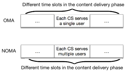
(a) A general illustration for the content delivery phase

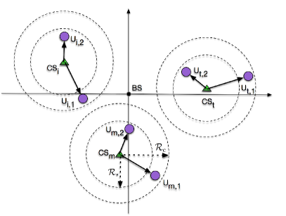
(b) An example for the outcome of content pushing

Figure 3: An illustration of the impact of NOMA on content delivery. In OMA, each content server serves a single user. By using NOMA, an additional user can be served.

III-B2 NOMA Assisted Content Delivery

If the NOMA principle is applied in the content delivery phase, each content server can serve two users. Thereby, it is assumed that each content server can find at least two users whose requests can be accommodated locally. This assumption is applicable to high-density wireless networks, such as networks deployed in sport stadiums or airports, where the number of users is much larger than the number of content servers. We note that this assumption constitutes the worst case for the reception reliability of the users. In fact, content servers that do not have any user to server will not cause interference to the users served by other content servers. Without loss of generality, assume that the two users are ordered based on their distances to the associated content server. As shown in Fig. 3, the far user, which is far from the content server and is denoted by $\text{U}_{m,1}$, is inside a ring bounded by radii $\mathcal{R}_{s}$ and $\mathcal{R}_{c}$, $\mathcal{R}_{s}<\mathcal{R}_{c}$. The near user, which is close to the content server and is denoted by $\text{U}_{m,2}$, is inside a disc with radius $\mathcal{R}_{s}$. Without loss of generality, denote the file requested by $\text{U}_{m,k}$ by $f_{m,k}$, $f_{m,k}\in\mathcal{F}$. Each content server broadcasts a superposition signal containing two messages, and $\text{U}_{m,k}$, which is associated with $\text{CS}_{m}$, receives the following signal:

$$y_{m,k}= \underset{\text{Signals from $\text{CS}_{m}$}}{\underbrace{\frac{h_{m,mk}}{\sqrt{L\left(||y_{m,k}||\right)}}\sum^{2}_{l=1}\alpha_{l}\bar{f}_{m,l}}}$$ (16)

$$+\underset{\text{Signals from interfering clusters}}{\underbrace{\sum_{x_{j}\in\Phi_{c}\backslash m}\frac{h_{j,mk}}{\sqrt{L\left(||y_{m,k}+x_{m}-x_{j}||\right)}}\sum^{2}_{l=1}\alpha_{l}\bar{f}_{j,l}}}+n_{m,k},$$

where $\bar{f}_{j,l}$ denotes the signal which represents the information contained in file ${f}_{j,l}$, $\alpha_{l}$ denotes the NOMA power allocation coefficient, $n_{m,k}$ is the additive complex Gaussian noise, and $h_{j,mk}$ denotes the Rayleigh fading channel coefficient between $\text{CS}_{j}$ and $\text{U}_{m,k}$. In order to obtain tractable analytical results, fixed power allocation is used, instead of CR power allocation, and it is assumed that all content servers use the same fixed power allocation coefficients. In order to keep the notations consistent, the power allocation coefficients are still denoted by $\alpha_{i}$. We note that the simulation results provided in Section V show that the use of this fixed power allocation can still ensure that NOMA outperforms OMA for both users.

$\text{U}_{m,1}$ will treat its partner’s message as noise and decode its own message $f_{m,1}$ with the following SINR:

$$\text{SINR}^{1}_{m,1}= \frac{\frac{\alpha_{1}^{2}|h_{m,m1}|^{2}}{L\left(||y_{m,1}||\right)}}{\frac{\alpha_{2}^{2}|h_{m,m1}|^{2}}{L\left(||y_{m,1}||\right)}+\text{I}^{m,1}_{inter}+\frac{1}{\rho}},$$ (17)

where

$$\text{I}^{m,1}_{inter}=\underset{x_{j}\in\Phi_{c}\backslash m}{\sum}\frac{|h_{j,m1}|^{2}}{L\left(||y_{m,1}+x_{m}-x_{j}||\right)}.$$

In practice, the content servers are expected to use less transmission power than the BS, but for notational simplicity, $\rho$ is still used to denote the ratio between the transmission power of the content servers and the noise power. In Section V, for the presented computer simulation results, different transmission powers are adopted for the BS and the content servers.

The near user, $\text{U}_{m,2}$, intends to first decode its partner’s message with the data rate $\log(1+\text{SINR}^{1}_{m,2})$, where $\text{SINR}^{1}_{m,2}$ is defined similarly to $\text{SINR}^{1}_{m,1}$, i.e., $\text{SINR}^{1}_{m,2}=\frac{\frac{\alpha_{1}^{2}|h_{m,m2}|^{2}}{L\left(||y_{m,2}||\right)}}{\frac{\alpha_{2}^{2}|h_{m,m2}|^{2}}{L\left(||y_{m,2}||\right)}+\text{I}^{m,2}_{inter}+\frac{1}{\rho}}$, and the inter-cluster interference, $\text{I}^{m,2}_{inter}$, is defined similarly to $\text{I}^{m,1}_{inter}$. If $\log(1+\text{SINR}^{1}_{m,2})>R_{1}$, i.e., $\text{U}_{m,2}$ can decode its partner’s message successfully, $\text{U}_{m,2}$ will remove $f_{m,1}$ and decode its own message with the following SINR:

$$\text{SINR}^{2}_{m,2}= \frac{\frac{\alpha_{2}^{2}|h_{m,m2}|^{2}}{L\left(||y_{m,2}||\right)}}{\text{I}^{m,2}_{inter}+\frac{1}{\rho}}.$$ (18)

The outage probabilities of the two users are defined as follows:

$$\mathrm{P}^{1}_{m,1}=\mathrm{P}(\log(1+\text{SINR}^{1}_{m,1})<R_{1}),$$ (19)

and

$$\mathrm{P}^{2}_{m,2}=1-\mathrm{P}(\log(1+\text{SINR}^{1}_{m,2})>R_{1},\log(1+\text{SINR}^{2}_{m,2})>R_{2}).$$ (20)

The following lemma provides closed-form expressions for these outage probabilities.

$\mathbf{Lemma}$ 3.

The outage probability of $\text{U}_{m,2}$ can be expressed as follows:

$$\mathrm{P}^{o}_{m,2}\approx 1-\sum^{N}_{n=1}\bar{w}_{n}e^{-\frac{c_{n,\mathcal{R}_{s}}\frac{1}{\rho}}{\tilde{\tau}}}q\left(\frac{c_{n,\mathcal{R}_{s}}}{\tilde{\tau}}\right),$$ (21)

where $\tilde{\tau}=\min\left\{\frac{\alpha^{2}_{1}-\epsilon_{1}\alpha^{2}_{2}}{\epsilon_{1}},\frac{\alpha^{2}_{2}}{\epsilon_{2}}\right\}$, $q(s)={\rm exp}\left(-2\pi\lambda_{c}\frac{s^{\frac{2}{\alpha}}}{\alpha}\text{B}\left(\frac{2}{\alpha},\frac{\alpha-2}{\alpha}\right)\right)$, $\text{B}(\cdot,\cdot)$ denotes the Beta function, $\bar{w}_{n}=\frac{\pi}{2N}\sqrt{1-w_{n}^{2}}\left(w_{n}+1\right)$, $w_{n}$ is defined in Lemma 2, and $c_{n,r}=\left(\frac{r}{2}w_{n}+\frac{r}{2}\right)^{\alpha}$.

The outage probability of $\text{U}_{m,1}$ can be expressed as follows:

$$\mathrm{P}^{o}_{m,1}\approx 1+\frac{\mathcal{R}_{s}^{2}}{\mathcal{R}_{c}^{2}-\mathcal{R}_{s}^{2}}\sum^{N}_{n=1}\bar{w}_{n}e^{-\frac{c_{n,\mathcal{R}_{s}}\frac{\epsilon_{1}}{\rho}}{\alpha^{2}_{1}-\epsilon_{1}\alpha^{2}_{2}}}q\left(e^{-\frac{c_{n,\mathcal{R}_{s}}\epsilon_{1}}{\alpha^{2}_{1}-\epsilon_{1}\alpha^{2}_{2}}}\right)$$ (22)

$$-\frac{\mathcal{R}_{c}^{2}}{\mathcal{R}_{c}^{2}-\mathcal{R}_{s}^{2}}\sum^{N}_{n=1}\bar{w}_{n}e^{-\frac{c_{n,\mathcal{R}_{c}}\frac{\epsilon_{1}}{\rho}}{\alpha^{2}_{1}-\epsilon_{1}\alpha^{2}_{2}}}q\left(e^{-\frac{c_{n,\mathcal{R}_{c}}\epsilon_{1}}{\alpha^{2}_{1}-\epsilon_{1}\alpha^{2}_{2}}}\right).$$

Proof.

See Appendix D. ∎

Remark 9: In the previous subsection, the CR power allocation policy is used and this type of power allocation ensures that the NOMA outage performance of the far user, $\text{U}_{m,1}$, is the same as that for OMA. Since fixed power allocation coefficients are used in this subsection for content pushing, the performance of the far user is no longer guaranteed, but surprisingly, our simulation results indicate that the use of NOMA can still yield an outage performance gain for the far user, compared to OMA, as shown in Section V.

IV Push-and-deliver Strategy

While the proposed push-then-deliver strategy ensures that more files can be pushed to the content servers during a short content pushing phase, it still relies on the same principle as conventional caching in the sense that content pushing and content delivery are separately carried out. Therefore, if the time interval between two adjacent content pushing phases is large, the caches of the content servers can be updated only infrequently. If new content arrives during the content delivery phase, the use of both conventional caching and the proposed push-then-deliver strategy means that the base station has to wait until the next content pushing phase in order to update the caches of the content servers. In contrast, the proposed push-and-deliver strategy provides an efficient mechanism for frequently updating the files cached at the content servers by exploiting opportunities for content pushing during the content delivery phase as illustrated in Fig. 4(a). In particular, such opportunities arise, when the BS has to serve a user directly during the content delivery phase, as explained in the following.

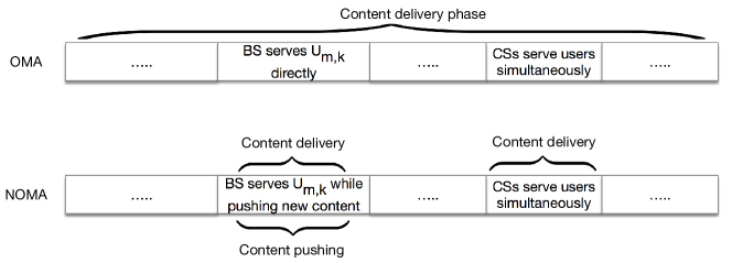
(a) General principle of push-and-deliver

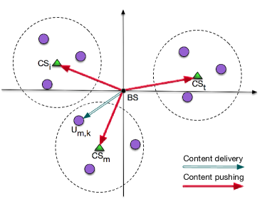
(b) An illustration of push-and-deliver

Figure 4: An illustration of the proposed push-and-deliver strategy.

In particular, consider a time slot which is dedicated to user $\text{U}_{m,k}$, as shown in Fig. 4(b). During this time slot, if OMA is used, only this user can be served by the BS directly. However, the use of the NOMA principle offers the opportunity to also push new content to the content servers, i.e., the BS sends a superposition signal containing the file requested by $\text{U}_{m,k}$, denoted by ${f}_{0}$, and the $M_{s}$ most popular files pushed by the BS, denoted by $f_{i}$, $1\leq i\leq M_{s}$. Assume that ${f}_{0}$ and $f_{i}$, $1\leq i\leq M_{s}$, belong to different file libraries, and the newly pushed files are useful to all the content servers, in order to avoid correlation among these files and to simplify the expression for the cache hit probability. This assumption is reasonable in practice and can be justified by using the following scenario as an example. Assume that after a period following the initial content pushing phase, one user needs to be served by the BS directly, and during this period, a new library of files, e.g., a set of videos for breaking news, has arrived at the BS to be pushed to the content servers. None of the content servers has had a chance to cache these files yet. With the proposed push-and-deliver strategy, the BS can push the new files to the content servers, while serving the requesting user directly, i.e., waiting for the next content pushing phase is avoided.

IV-A Performance Analysis

Following similar steps as in the previous section, the data rate of $\text{U}_{m,k}$ for decoding its requested file, $f_{0}$, which is directly sent by the BS, is given by

$$\text{R}_{m,k}= \log\left(1+\frac{\frac{\alpha_{0}^{2}|h_{mk}|^{2}}{L\left(||y_{m,k}+x_{m}||\right)}}{\sum^{M_{s}}_{l=1}\frac{\alpha_{l}^{2}|h_{mk}|^{2}}{L\left(||y_{m,k}+x_{m}||\right)}+\frac{1}{\rho}}\right),$$ (23)

and each content server, $\text{CS}_{m}$, can decode the additionally pushed file $f_{i}$ with the following data rate:

$$\text{R}^{l}_{m}= \log\left(1+\frac{\frac{\alpha_{l}^{2}}{L\left(||x_{m}||\right)}}{\sum^{M_{s}}_{l=i+1}\frac{\alpha_{l}^{2}}{L\left(||x_{m}||\right)}+\frac{1}{\rho}}\right),$$ (24)

if $\text{R}^{j}_{m}$ is larger than $R_{j}$, for $0\leq j\leq i-1$, where $R_{l}$ denotes the target data rate of $f_{l}$. Again, small scale multi-path fading is not considered in the channel model for $\text{CS}_{m}$, as we assume that the large scale path loss is dominant in this case, but small scale fading is considered for the users’ channels. Note that the indices of the power allocation coefficients $\alpha_{i}$ start from $0$, due to file $f_{0}$. Compared to the distance between $\text{CS}_{m}$ and the BS, the corresponding distance between $\text{U}_{m,k}$ and the BS has a very complicated pdf, as shown in the following subsection. Therefore, in order to obtain tractable analytical results, fixed power allocation coefficients $\alpha_{i}$ will be used, instead of the CR based ones. The outage probabilities of the user and the content servers will be studied in the following subsections, respectively.

IV-A1 Performance of the user

The main challenge in analyzing the outage performance at the user is the complicated expression for the pdf of the distance $||y_{m,k}+x_{m}||$. First, we define $\bar{z}_{m,k}=\frac{|h_{mk}|^{2}}{L\left(||y_{m,k}+x_{m}||\right)}$. The outage probability at the user can be expressed as follows:

$$\mathrm{P}_{m,k}^{1}= \mathrm{P}(\text{R}_{m,k}<R_{0})=\mathrm{P}\left(\bar{z}_{m,k}<\frac{{\epsilon}_{0}}{\rho\zeta_{1}}\right)$$ (25)

$$= \mathcal{E}_{L\left(||y_{m,k}+x_{m}||\right)}\left\{1-e^{-L\left(||y_{m,k}+x_{m}||\right)\frac{{\epsilon}_{0}}{\rho\zeta_{0}}}\right\},$$

where $\zeta_{l}=\alpha^{2}_{l}-{\epsilon}_{l}\sum^{M_{s}}_{j=l+1}\alpha^{2}_{j}$ for $0\leq l<M_{s}$, and $\zeta_{M_{s}}=\alpha^{2}_{M_{s}}$. Again, it is assumed that the power allocation coefficients and the target data rates are carefully chosen to ensure that $\zeta_{l}$ is positive.

In order to derive the pdf of $||y_{m,k}+x_{m}||$, we first define $r_{m}=||x_{m}||$ and also a function

$$g(r_{m},r)=\frac{2r\arccos\frac{r_{m}^{2}+r^{2}-\mathcal{R}_{c}^{2}}{2r_{m}r}}{\pi\mathcal{R}_{c}^{2}}.$$

Conditioned on $r_{m}$, the pdf of $||y_{m,k}+x_{m}||$ is given by [38]

$$f_{||y_{m,k}+x_{m}||}(r|r_{m})=g(r_{m},r),$$ (26)

for $r_{m}-\mathcal{R}_{c}\leq r\leq r_{m}+\mathcal{R}_{c}$, if $r_{m}>\mathcal{R}_{c}$. Otherwise, we have

$$\begin{array}[]{ll}&f_{||y_{m,k}+x_{m}||}(r|r_{m})\\ =&\left\{\begin{array}[]{ll}2\pi r,&\text{if }r\leq\mathcal{R}_{c}-r_{m}\\ 2\pi r-g(r_{m},r),&\text{if }\mathcal{R}_{c}-r_{m}<r\leq\sqrt{\mathcal{R}_{c}^{2}-r_{m}^{2}}\\ g(r_{m},r),&\text{if }\sqrt{\mathcal{R}_{c}^{2}-r_{m}^{2}}<r\leq\mathcal{R}_{c}+r_{m}\end{array}\right..\end{array}$$ (32)

In order to avoid the trivial cases, which lead to $r=0$, i.e., the user is located at the same place as the BS, we assume that no content server can be located inside the disc, denoted by $\mathcal{B}(x_{0},\delta\mathcal{R}_{c})$, i.e., a disc with the BS located at its origin and radius $\delta\mathcal{R}_{c}$ with $\delta>1$, which means that $r_{m}\geq\delta\mathcal{R}_{c}$ for all $m\geq 1$. Therefore, only the expression in (26) needs to be used since $r_{m}$ is strictly larger than $\mathcal{R}_{c}$.

After using the pdf of $||y_{m,k}+x_{m}||$, the outage probability can be expressed as follows:

$$\mathrm{P}_{m,k}^{1}= 1-\int_{\delta\mathcal{R}_{c}}^{\infty}\int^{z+\mathcal{R}_{c}}_{z-\mathcal{R}_{c}}e^{-\frac{{\epsilon}_{0}r^{\alpha}}{\rho\zeta_{0}}}g(z,r)dr\bar{f}_{r_{m}}(z)dz,$$ (33)

where $\bar{f}_{r_{m}}(z)$ denotes the pdf of $r_{m}$. Because of the assumption that no content server can be located inside of $\mathcal{B}(x_{0},\delta\mathcal{R}_{c})$, the pdf of $r_{m}$ is different from that in (55), but the steps of the proof for Theorem 1 in [39] can still be applied to obtain the pdf of $r_{m}$. Particularly, first denote by $\mathcal{A}_{r}$ the ring with inner radius $\delta\mathcal{R}_{c}$ and outer radius $r$. The cumulative distribution function (CDF) of $r_{m}$ can be expressed as follows:

$$\tilde{F}_{r_{m}}(r)= 1-\mathrm{P}(\#\text{ of nodes in the ring }\mathcal{A}_{r}<m)$$ (34)

$$= 1-\sum^{m-1}_{l=0}\frac{(\lambda_{c}[\pi r^{2}-\pi\delta^{2}\mathcal{R}_{c}^{2}])^{l}}{l!}e^{-\lambda_{c}[\pi r^{2}-\pi\delta^{2}\mathcal{R}_{c}^{2}]}.$$

Therefore, the pdf of $r_{m}$ can be calculated as follows:

$$\bar{f}_{r_{m}}(r)= -2\pi\lambda_{c}re^{-\lambda_{c}[\pi r^{2}-\pi\delta^{2}\mathcal{R}_{c}^{2}]}\left(\sum^{m-1}_{l=1}\frac{(\lambda_{c}[\pi r^{2}-\pi\delta^{2}\mathcal{R}_{c}^{2}])^{l-1}}{(l-1)!}\right.$$

$$\left.-\sum^{m-1}_{l=0}\frac{(\lambda[\pi r^{2}-\pi\delta^{2}\mathcal{R}_{c}^{2}])^{l}}{l!}\right)$$

$$= 2\pi\lambda_{c}^{m}re^{-\lambda_{c}[\pi r^{2}-\pi\delta^{2}\mathcal{R}_{c}^{2}]}\frac{[\pi r^{2}-\pi\delta^{2}\mathcal{R}_{c}^{2}]^{m-1}}{(m-1)!}.$$ (35)

Substituting (IV-A1) into (33), the outage probability of the user can be obtained.

IV-A2 Performance of the content servers

The content servers need to carry out SIC in order to decode the newly pushed files $f_{l}$. As a result, the outage probability of $\text{CS}_{m}$ for decoding $f_{i}$ can be expressed as follows:

$$\mathrm{P}_{m}^{i}= 1-\mathrm{P}(\text{R}_{m}^{l}>R_{l},\forall l\in\{0,\cdots,i\})$$ (36)

$$= \mathrm{P}\left(L(||x_{m}||)>\min\left\{\frac{\rho\zeta_{l}}{{\epsilon}_{l}},\forall l\in\{0,\cdots,i\}\right\}\right).$$

By applying the assumption that $r_{m}\geq\delta\mathcal{R}_{c}$ and also the pdf in (IV-A1), the outage probability of $\text{CS}_{m}$ for decoding $f_{i}$ can be expressed as follows:

$$\mathrm{P}_{m}^{i}= \sum^{m-1}_{l=0}\frac{(\lambda_{c}\left[\frac{\pi}{\bar{\tau}_{i}^{2}}-\pi\delta^{2}\mathcal{R}_{c}^{2}\right])^{l}}{l!}e^{-\lambda_{c}\left[\frac{\pi}{\bar{\tau}_{i}^{2}}-\pi\delta^{2}\mathcal{R}_{c}^{2}\right]},$$ (37)

where $\bar{\tau}_{i}=\left(\frac{1}{\min\left\{\frac{\rho\zeta_{l}}{{\epsilon}_{l}},\forall l\in\{0,\cdots,i\}\right\}}\right)^{\frac{1}{\alpha}}$.

Based on the outage probability $\mathrm{P}_{m}^{i}$, the corresponding cache hit probability for a user associated with $\text{CS}_{m}$ can be expressed as follows:

$$\mathrm{P}^{hit}_{m}=\sum^{M_{s}}_{i=1}\mathrm{P}(f_{i})(1-\mathrm{P}_{m}^{i}),$$ (38)

where $f_{0}$ has been omitted as it is the file currently requested by a user and it is assumed that $f_{0}$ and $f_{l}$, $1\leq l\leq M_{s}$, belong to different libraries.

IV-B OMA Benchmarks

A naive OMA based benchmark is that the BS does not push new content while serving a user directly. Compared to this naive OMA scheme, the benefit of the proposed push-and-deliver strategy is obvious since new content is delivered and the cache hit probability will be improved.

A more sophisticated OMA scheme is to divide a single time slot into $(M_{s}+1)$ sub-slots. During the first sub-slot, the user is served directly by the BS. From the second until the $(M_{s}+1)$-th sub-slots, the BS will individually push the files, $f_{i}$, $i\in\{1,\cdots,M_{s}\}$, to the content servers. Compared to this more sophisticated OMA scheme, the use of the proposed push-and-deliver strategy still offers a significant gain in terms of the cache hit probability, as will be shown in Section V.

IV-C Extension to D2D Caching

The aim of this subsection is to show that the concept of push-and-deliver can also be applied to D2D caching. Assume that a time slot is dedicated to a user whose request cannot be found in the caches of its neighbours, and during this time slot, the BS will send the requested file ${f}_{0}$ to the user directly. By applying the push-and-deliver strategy, the BS will also proactively push $M_{s}$ new files, $f_{l}$, $1\leq l\leq M_{s}$, to all users for future use. In other words, when the BS addresses the current demand of a user directly, the BS pushes more content files to all users, including the user which requests $f_{0}$, for future use.

In the context of D2D caching, content servers are no longer needed. Therefore, the spatial model presented in Section II needs to be revised accordingly. Particularly, it is assumed that the locations of the users are denoted by $y_{k}$ and modelled as an HPPP, denoted by $\Phi_{u}$, with density $\lambda_{u}$.

After implementing the push-and-deliver strategy, following similar steps as in the previous subsection, for a user with distance $r$ from the BS and Rayleigh fading channel gain $h$, the outage probability for decoding $f_{i}$ is given by

$$\text{R}^{i}_{r}= \log\left(1+\frac{\alpha_{i}^{2}|h|^{2}r^{-\alpha}}{\sum^{M_{s}}_{j=i+1}\alpha_{j}^{2}|h|^{2}r^{-\alpha}+\frac{1}{\rho}}\right),$$ (39)

when $\text{R}^{l}_{r}>R_{l}$, for $0\leq l\leq i-1$. If $f_{j}$, $0\leq j\leq M_{s}-1$, can be decoded correctly, $f_{M_{s}}$ can be decoded by this user with the following data rate:

$$\text{R}^{M_{s}}_{r}= \log\left(1+\rho\alpha_{M_{s}}^{2}|h|^{2}r^{-\alpha}\right).$$ (40)

Consequently, for a user with distance $r$ from the BS, the probability of successfully decoding $f_{i}$ can be expressed as follows:

$$\mathrm{P}^{i}(r)= \mathrm{P}\left(\text{R}^{l}_{r}>R_{l},\forall l\in\{0,\cdots,i\}\right)$$ (41)

$$= e^{-\bar{\tau}_{i}^{\alpha}r^{\alpha}}.$$

Following (41), one can draw the conclusion that the locations of the users which can successfully receive $f_{i}$ no longer follow the original HPPP with $\lambda_{u}$, but follow an inhomogeneous PPP which is thinned from the original HPPP by $\mathrm{P}^{i}(r)$, i.e., the density of this new PPP is $\mathrm{P}^{i}(r)\lambda_{u}$. By using this thinning process, the cache miss probability can be characterized as follows.

During the D2D content delivery phase, assume a newly arrived user, whose location is denoted by $y_{0}$, requests file $f_{i}$. Denote by $\mathcal{B}(y_{0},d)$ a disc with radius $d$ and its origin located at $y_{0}$. This disc is the area in which the user searches for a helpful neighbour which has the requested file in its cache. For this inhomogeneous PPP, the cache hit probability for the user requesting $f_{i}$ is given by

$$\mathrm{P}^{hit}_{i}= 1-\mathrm{P}(\text{no user in }\mathcal{B}(y_{0},d)\text{ caches }f_{i})$$ (42)

$$= 1-e^{-\Lambda_{i}(\mathcal{B}(y_{0},d))},$$

where $\Lambda_{i}(\mathcal{B}(y_{0},d))$ denotes the intensity measure of the inhomogeneous PPP for the users which have $f_{i}$ in their caches. In (42), the hit probability is found by determining the cache miss probability which corresponds to the event that the user cannot find its requested file in the caches of its neighbours located in the disc $\mathcal{B}(y_{0},d)$. The calculation of the cache hit probability depends on the relationship between $d$ and the distance between the observing user and the BS, denoted by $r_{0}$, as shown in the following subsections.

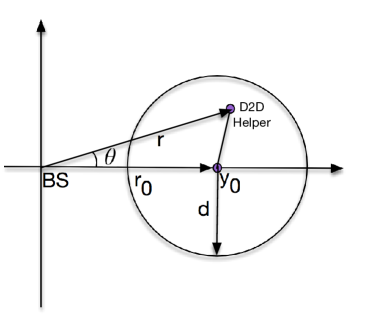
(a) $d<r_{0}$

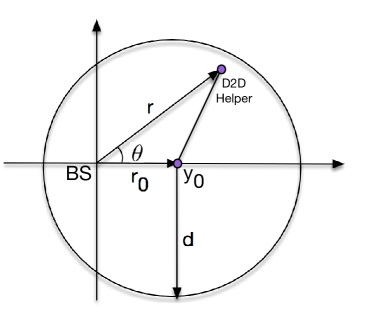
(b) $d\geq r_{0}$

Figure 5: Two possible cases between the radius of the search disc, $\mathcal{B}(y_{0},d)$, and the distance between the observing user located at $y_{0}$ and the BS.

IV-C1 For the case of $d<r_{0}$

For $d<r_{0}$, define $\Lambda_{i}(\mathcal{B}(y_{0},d))\triangleq\Lambda^{i}_{d\leq r_{0}}(r_{0})$. The assumption $d<r_{0}$ means that the BS is excluded from $\mathcal{B}(y_{0},d)$. Therefore, the intensity measure can be calculated as follows:

$$\Lambda^{i}_{d\leq r_{0}}(r_{0}) =\underset{{r,\theta\in\mathcal{B}(y_{0},d)}}{\int\int}\mathrm{P}^{i}(r)\lambda_{u}d\theta rdr.$$ (43)

As can be observed from Fig. 5, the constraint on $r$ and $\theta$ can be expressed as follows:

$$r^{2}+r_{0}^{2}-2r_{0}r\cos\theta\leq d^{2}.$$ (44)

Therefore, the intensity measure can be expressed as follows:

$$\Lambda^{i}_{d\leq r_{0}}(r_{0}) =\int^{r_{0}+d}_{r_{0}-d}\int^{\arccos\frac{r^{2}+r_{0}^{2}-d^{2}}{2r_{0}r}}_{-\arccos\frac{r^{2}+r_{0}^{2}-d^{2}}{2r_{0}r}}\mathrm{P}^{i}(r)\lambda_{u}d\theta rdr$$

$$=2\lambda_{u}\int^{r_{0}+d}_{r_{0}-d}\mathrm{P}^{i}(r)r\arccos\frac{r^{2}+r_{0}^{2}-d^{2}}{2r_{0}r}dr.$$ (45)

By applying Chebyshev-Gauss quadrature, the intensity measure can be calculated as follows:

$$\Lambda^{i}_{d\leq r_{0}}(r_{0}) \approx 2\lambda_{u}d\sum^{N}_{l=1}\frac{\pi}{N}g_{r}\left(r_{0}+dw_{l}\right)\sqrt{1-w_{l}^{2}},$$ (46)

where $g_{r}(z)$ is given by

$$g_{r}(z)=\mathrm{P}^{i}(z)z\arccos\frac{z^{2}+r_{0}^{2}-d^{2}}{2r_{0}z}.$$ (47)

IV-C2 For the case of $d\geq r_{0}$

For $d\geq r_{0}$, define $\Lambda^{i}(\mathcal{B}(y_{0},d))\triangleq\Lambda_{d>r_{0}}$. The assumption, $d\geq r_{0}$, means that the BS is inside of $\mathcal{B}(y_{0},d)$. Following similar steps as in the previous case, the intensity measure can be evaluated as follows:

$$\Lambda^{i}_{d\leq r_{0}}(r_{0})= \int_{0}^{d-r_{0}}\int^{\pi}_{-\pi}\mathrm{P}_{i}(r)\lambda_{u}d\theta rdr$$

$$+\int^{r_{0}+d}_{d-r_{0}}\int^{\arccos\frac{r^{2}+r_{0}^{2}-d^{2}}{2r_{0}r}}_{-\arccos\frac{r^{2}+r_{0}^{2}-d^{2}}{2r_{0}r}}\mathrm{P}_{i}(r)\lambda_{u}d\theta rdr$$

$$\approx \frac{2\pi\lambda_{u}}{\alpha\bar{\tau}_{i}^{2}}\gamma\left(\frac{2}{\alpha},\bar{\tau}_{i}^{\alpha}(d-r_{0})^{\alpha}\right)$$

$$+2\lambda_{u}r_{0}\sum^{N}_{l=1}\frac{\pi}{N}g_{r}\left(d+r_{0}w_{l}\right)\sqrt{1-w_{l}^{2}},$$ (48)

where $\gamma(\cdot)$ denotes the incomplete Gamma function, and the approximation in the last step follows from the application of Chebyshev-Gauss quadrature.

Finally, the cache hit probability can be obtained by substituting (46) and (48) into (42).

V Numerical Studies and Discussions

In this section, the performances achieved by the proposed push-then-deliver and push-and-deliver strategies are studied by using computer simulations, where the accuracy of the developed analytical results will be also verified. The system parameters adopted for simulation and analysis are specified in the captions of the figures shown in this section.

V-A Performance of Push-then-deliver Strategy

In Figs. 6 and 7, the impact of the NOMA assisted push-then-deliver strategy on the cache hit probability is studied. The thermal noise is set as $\sigma_{n}^{2}=-100$ dBm. The density of the content servers is parameterized by cluster radius $\mathcal{R}_{c}$, i.e., $\lambda_{c}=\frac{0.01}{\pi\mathcal{R}_{c}^{2}}$, in order to account for the fact that the density of the content servers is affected by $\mathcal{R}_{c}$. By applying the NOMA principle to the content pushing phase, more content can be pushed to the content servers simultaneously, and hence, the cache hit probability is improved, compared to the OMA case, as can be observed from Fig. 6. For example, when the transmission power is $40$ dBm, the shape parameter for the content popularity is $\gamma=0.5$, and $\mathcal{R}_{c}=50$ m, the use of OMA yields a hit probability of $0.2$, and the use of NOMA improves this value to $0.45$, which corresponds to a $100\%$ improvement. At low SNR, NOMA and OMA yield the same performance. This is due to the use of the CR inspired power allocation policy in (7), which implies that at low SNR, all the power is allocated to file $f_{1}$, and hence, there is no difference between the OMA and NOMA schemes. Note that the curves for analysis and simulation match perfectly in Fig. 6, which demonstrates the accuracy of the developed analytical results. Furthermore, we note that the NOMA power allocation coefficients $\beta_{i}$ are assumed to be fixed. Optimizing these power allocation coefficients dynamically according to the users’ channel conditions can further enhance the performance gain of NOMA assisted caching compared to the OMA baseline scheme.

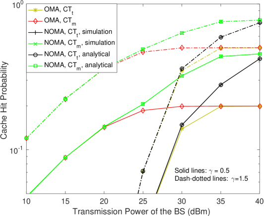
(a) $\mathcal{R}_{c}=100$m

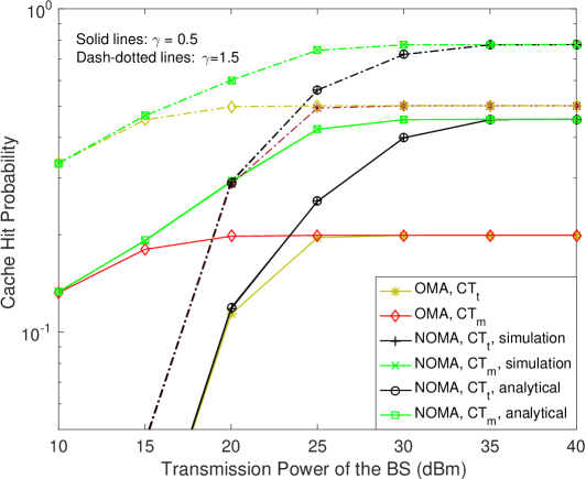
(b) $\mathcal{R}_{c}=50$m

Figure 6: The cache hit probability for the push-then-deliver strategy. $N=20$, $\alpha=3$, $\lambda_{c}=\frac{0.01}{\pi\mathcal{R}_{c}^{2}}$, $t=5$, $m=1$, $M_{s}=3$, and $R_{l}=1$ bit per channel use (BPCU), for $1\leq l\leq 3$. The power allocation coefficient for file $f_{1}$ is based on the CR power allocation policy. The power allocation coefficients for files $f_{2}$ and $f_{3}$ are $\beta_{2}=\frac{3}{4}$ and $\beta_{3}=\frac{1}{4}$, respectively. $|\mathcal{F}|=10$.

The impact of $\gamma$, the shape parameter defining the content popularity, on the hit probability is significant, as can be observed in Fig. 6. Particularly, increasing the value of $\gamma$ improves the hit probability. This is because a larger value of $\gamma$ implies that the first $M_{s}$ files become more popular, hence ensuring the delivery of these more popular files can significantly improve the hit probability, as indicated by (9). Comparing Fig. 6(a) with Fig. 6(b), one can observe that the impact of $\mathcal{R}_{c}$ on the hit probability is also significant, which is due to the fact that the density of the content servers depends on $\mathcal{R}_{c}$. Particularly, a larger $\mathcal{R}_{c}$ means that the content servers are more sparsely deployed and hence it is more difficult for the BS to push content to the content servers, and the cache hit probability decreases.

Recall that during the time slot considered for content pushing in Section III-A, the BS pushes additional files to $\text{CS}_{m}$ while ensuring that $f_{1}$ is pushed to $\text{CS}_{t}$. In Fig. 7, the impact of different choices of $m$ and $t$ on the cache hit probability is studied. As can be observed from the figure, increasing $t$ will decrease the hit probability. This is again due to the use of the CR power allocation policy. In particular, a larger $t$ means that more transmission power is needed to delivery $f_{1}$ to $\text{CS}_{t}$, and hence, less power is available for other files. An interesting observation in Fig. 7 is that the shape of the hit probability curves is not smooth. This is due to the fact that the hit probability is the summation of popularity probabilities $P(f_{l})$ and these popularity probabilities are prefixed and not continuous, as shown in (1). On the other hand, for a fixed $t$, increasing $m$ reduces the cache hit probability, since increasing $m$ means that $\text{CS}_{m}$ is further away from the BS and hence its reception reliability deteriorates.

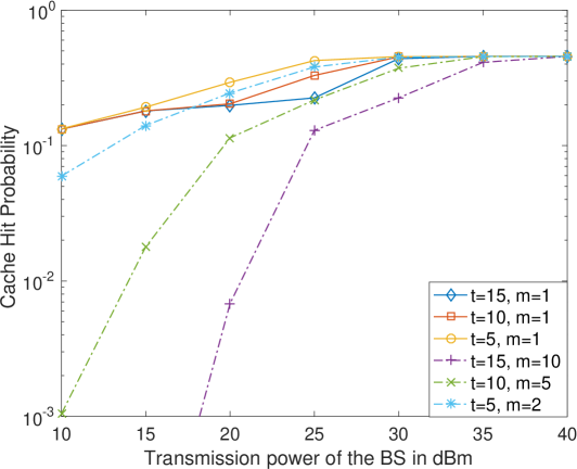
Figure 7: The impact of the choices of $m$ and $t$ on the cache hit probabilities for the push-then-deliver strategy. $N=20$, $\alpha=3$, $\mathcal{R}_{c}=50$m, $\lambda_{c}=\frac{0.01}{\pi\mathcal{R}_{c}^{2}}$, ${M_{s}}=3$, $t=5$, $m=1$, and $R_{l}=1$ BPCU, for $1\leq l\leq 3$. The power allocation coefficient for file $f_{1}$ is based on the CR power allocation policy. The power allocation coefficients for files $f_{2}$ and $f_{3}$ are $\beta_{2}=\frac{3}{4}$ and $\beta_{3}=\frac{1}{4}$, respectively. $\gamma=0.5$ and $|\mathcal{F}|=3$. Analytical results are used to generate the figure.

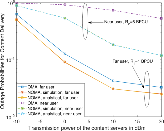
(a) $\alpha=3$

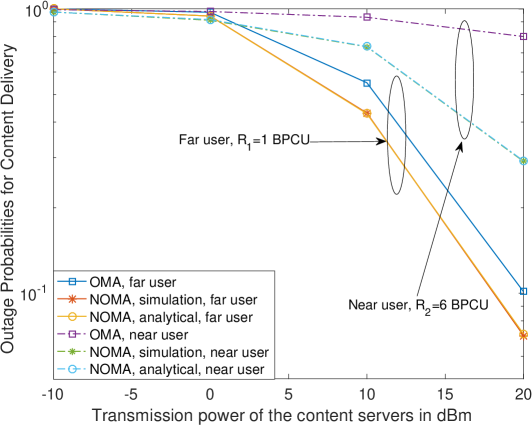
(b) $\alpha=4$

Figure 8: The outage probabilities for content delivery for the push-then-deliver strategy. $N=20$, $\alpha=4$, $\mathcal{R}_{c}=100$m. $\lambda_{c}=\frac{0.01}{\pi\mathcal{R}_{c}^{2}}$, $R_{1}=1$ BPCU, and $R_{2}=6$ BPCU. The power allocation coefficients are $\alpha_{1}^{2}=\frac{3}{4}$ and $\alpha_{2}^{2}=\frac{1}{4}$.

In Fig. 8, the impact of using NOMA for content delivery is studied, where the rate pair $\{R_{1},R_{2}\}$ is set to $\{1,6\}$ BPCU to account for the fact that the near user can achieve a higher data rate. As can be observed from the figure, the proposed push-then-deliver strategy can improve the reliability of content delivery, particularly for the user with strong channel conditions. For example, when the path loss exponent is set to $\alpha=3$ and the transmission power of the content servers is $20$ dBm, the use of NOMA ensures that the outage probability for the far user is improved from $4.5\times 10^{-2}$ to $3\times 10^{-2}$, which is a relatively small performance gain. However, the performance gap between the OMA and NOMA schemes for the near user is much larger, e.g., for the same case as considered before, the outage probability is improved from $5\times 10^{-1}$ to $1.1\times 10^{-2}$. Note that the outage probability for content delivery has an error floor, i.e., increasing the transmission power of the content severs cannot reduce the outage probability to zero. This is because multiple content servers transmit simultaneously, and hence, content delivery becomes interference limited at high SNR. We note that the impact of the path loss exponent on the reliability of content delivery is significant, as can be observed by comparing Figs. 8(a) and 8(b). This is due to the fact that a smaller value of $\alpha$ results in a lower path loss, which leads to an improved reception reliability.

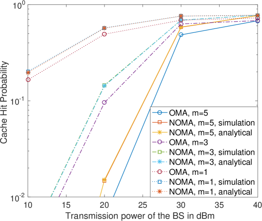
(a) Case 1

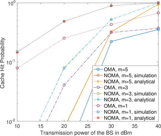
(b) Case 2

Figure 9: The cache hit probability for the proposed push-and-deliver strategy. $\mathcal{R}_{c}=50$m, $N=20$, $\gamma=1.5$, $\alpha=3$, $\lambda_{c}=\frac{0.01}{\pi\mathcal{R}_{c}^{2}}$, $M_{s}=3$, $\delta=1.1$. $R_{0}=\frac{1}{8}$ BPCU, $R_{1}=\frac{3}{4}$ BPCU, $R_{2}=\frac{7}{8}$ BPCU, and $R_{3}=\frac{11}{4}$ BPCU. The power allocation coefficients are $\alpha_{0}^{2}=\frac{4}{8}$, $\alpha_{1}^{2}=\frac{3}{8}$, $\alpha_{2}^{2}=\frac{2}{8}$, and $\alpha_{3}^{2}=\frac{1}{8}$.

V-B Performance of Push-and-deliver Strategy

In Fig. 9, the impact of the proposed push-and-deliver strategy on the cache hit probability is studied. We employ $\delta=1.1$ to avoid the trivial case where the user is located at the same place as the BS, as discussed in Section IV-A. As can be observed, the use of the proposed strategy can effectively improve the cache hit probability compared to the OMA case, which is consistent with the conclusions drawn in the previous subsection. In both sub-figures of Fig. 9, the analytical results perfectly match the simulation results, which verifies the accuracy of the developed analysis.

In Fig. 9, the impact of different choices for the popularity parameters on the cache hit probability is studied. In particular, the following two cases are considered:

• Case 1: ${\mathcal{F}}_{1}=\{f_{1},\cdots,f_{10}\}$, and the power allocation coefficient for $f_{l}$ is $\alpha_{l}$;

• Case 2: ${\mathcal{F}}_{2}=\{f_{1},\cdots,f_{3}\}$, and the power allocation coefficient for $f_{l}$ is $\alpha_{4-l}$.

The two cases correspond to two different options for mapping files with different popularities to different power levels (or equivalently SIC decoding orders), where in the first case, more popular files are assigned more power, and in the second case, less power is assigned to more popular files.

In Case 1, the performance gap between NOMA and OMA is not significant, as can be observed from Fig. 9(a). For example, when the transmit power is $40$ dBm and $m=5$, the use of OMA results in a hit probability of $0.7$ and the use of NOMA yields a hit probability of $0.8$, where the gap is $0.1$ only. However, for a different set of popularity parameters, i.e., Case 2, the performance gap between OMA and NOMA is significantly increased. For example, for a transmit power of $40$ dBm and $m=5$, the performance gap between OMA and NOMA is enlarged to $0.5$. The reason behind this phenomenon is as follows. Recall that the use of NOMA can significantly improve the reception reliability of the files which are decoded at the later stages of the SIC procedure, but the improvement for the files which are decoded during the first few stages of SIC is not significant. In Case 1, the first few files will get larger weights in the sum of the cache hit probability, i.e., file $f_{l}$, for a small $l$, has more impact on the overall performance. As a result, the gap between OMA and NOMA in Case 1 is small, since the reception reliability for decoding these files in the case of NOMA is not so different from that for OMA. On the other hand, Case 2 means that the most popular file, $f_{1}$, will be decoded last. As discussed before, the capabilities of OMA and NOMA to decode $f_{1}$ are quite different, which is the reason for the larger performance gap in Case 2.

Recall that the key idea of the push-and-deliver strategy is to perform content pushing when asking the BS to serve the users directly. Fig. 9 clearly demonstrates that this strategy can efficiently push new content to the content servers, but it does not demonstrate the impact of this strategy on content delivery, which is studied in Fig. 10. Particularly, as can be observed from the figure, the use of the proposed push-and-deliver strategy does not degrade the reception reliability of content delivery. In fact, the use of NOMA can even improve the outage probability for content delivery.

In Fig. 11, the concept of the proposed push-and-deliver strategy is extended to D2D caching scenarios. Without loss of generality, the newly arrived user is located at $y_{0}=(500\rm{m},500m)$. As expected, the use of the proposed strategy can significantly reduce the miss probability, compared to the case of OMA. For example, for the case where the user density is $\lambda_{u}=5\times 10^{-5}$, a transmit power of $40$ dBm, and $d=150$ m, the use of NOMA yields a miss probability of $6\times 10^{-2}$, whereas the miss probability for OMA is $1.6\times 10^{-1}$, which is much worse. As can be observed from the figure, increasing the value of $d$ can reduce the miss probability, since the area for searching for a D2D helper is increased. Another important observation is that by increasing the density of the users, the miss probability can be further reduced, since increasing the density means that more users are located in the same area and hence it is more likely to find a D2D helper. We note that, in Fig. 11, computer simulation and analytical results match perfectly, which demonstrates again the accuracy of the developed analysis.

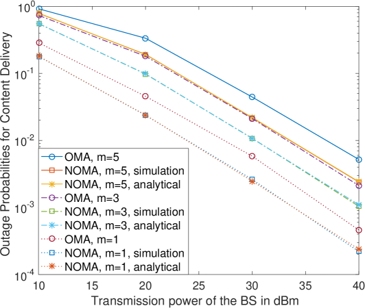
Figure 10: The impact of the push-and-deliver strategy on content delivery. $\mathcal{R}_{c}=50$m, $\gamma=1.5$, $\alpha=3$, $\lambda_{c}=\frac{0.01}{\pi\mathcal{R}_{c}^{2}}$, $M_{s}=3$, $N=20$, $\delta=1.1$. $R_{0}=\frac{1}{8}$ BPCU, $R_{1}=\frac{3}{4}$ BPCU, $R_{2}=\frac{7}{8}$ BPCU, and $R_{3}=\frac{11}{4}$ BPCU. The power allocation coefficients are $\alpha_{0}^{2}=\frac{4}{8}$, $\alpha_{1}^{2}=\frac{3}{8}$, $\alpha_{2}^{2}=\frac{2}{8}$, and $\alpha_{3}^{2}=\frac{1}{8}$. Case 2 is considered.

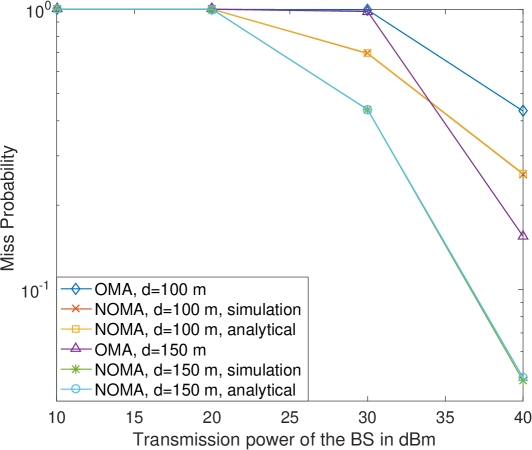
(a) $\lambda_{u}=5\times 10^{-5}$

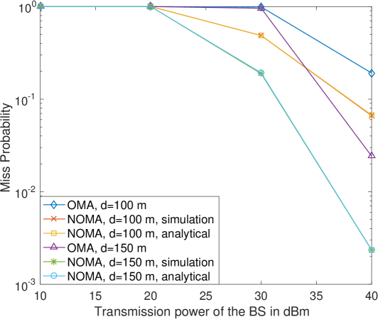
(b) $\lambda_{u}=1\times 10^{-4}$

Figure 11: The impact of the proposed push-and-deliver strategy on the cache miss probability in D2D caching scenarios. $N=20$, $\alpha=3$, $y_{0}=$ (500 m, 500 m), $R_{0}=0.5$ BPCU, $R_{1}=4$ BPCU and $M_{s}=1$. The power allocation coefficients are $\alpha_{0}^{2}=\frac{3}{4}$ and $\alpha_{1}^{2}=\frac{1}{4}$.

VI Conclusions

Unlike conventional wireless caching strategies which rely on the use of off-peak hours for content pushing, in this paper, the NOMA principle has been applied to wireless caching to enable the frequent update of the local caches via wireless transmission during on-peak hours. Two NOMA assisted caching strategies have been developed, namely the push-then-deliver strategy and the push-and-deliver strategy. The push-then-deliver strategy is applicable to the case when the content pushing phase and the content delivery phase are separated, and utilizes the NOMA principle independently in both phases. The developed analytical results demonstrate that the proposed NOMA assisted caching scheme can efficiently improve the cache hit probability and reduce the delivery outage probability. The push-and-deliver strategy is motivated by the fact that, in practice, it is inevitable that some user requests cannot be accommodated locally and the BS has to serve these users directly. The key idea of the push-and-deliver strategy is to merge the two phases, i.e., the BS pushes content to the content servers while simultaneously serving users directly. Furthermore, in addition to the caching scenario with caching infrastructure, e.g., content servers, we have considered D2D caching, where the use of NOMA has also been shown to yield superior performance compared to OMA.

The results in this paper open several new directions for future research. First, in this paper, the file popularity parameter has been assumed to be given and fixed. As demonstrated in Fig. 9, different choices for this parameter yield different cache hit probabilities, which means that dynamically optimizing the NOMA power allocation (or equivalently the NOMA SIC decoding order) for given content popularity parameters could further improve the performance of NOMA-assisted caching. Second, fixed NOMA power allocation coefficients have been adopted in this paper, except for Section III-A2, where CR inspired power allocation was used. In general, optimizing the power allocation coefficients is expected to further improve the performance of NOMA based caching. Third, increasing the density of the users or the search area in D2D caching can increase the cache hit probability, but might also cause stronger interference during the content delivery phase, when the D2D helpers deliver the requested files to their neighbours simultaneously. Therefore, for the content delivery phase, it is important to design low-complexity algorithms for efficient scheduling of the users’ requests in order to limit co-channel interference. In this context, coordinated multi-point transmission (CoMP) and cloud radio access networks (C-RAN) are interesting options for suppressing co-channel interference [40, 25]. Fourth, in this paper, content pushing is carried out without exploiting the structure of the content files. As shown in [22], the spectral efficiency of wireless caching can be further improved by applying coded caching, since only parts of the content files need to be cached and one multicast transmission during the content delivery phase can benefit multiple users simultaneously. Thus, enhanced caching and delivery schemes combining the benefits of the proposed NOMA based strategies and coded caching are of interest. Fifth, in this paper, the cache hit probability has been used as the performance criterion, whereas latency is another important metric [41, 42, 43]. The proposed caching strategies can potentially decrease the latency for content delivery. On the one hand, the proposed push-then-deliver strategy can effectively reduce the waiting time of the users for being served, since multiple users can be simultaneously served by one content server. On the other hand, with the proposed push-and-deliver strategy, the files cached at the content servers can be updated more frequently, which indirectly helps in reducing the latency of content delivery. Hence, a formal analysis of the impact of the proposed caching strategies on the latency of content delivery is needed, where various effects have to be considered, including the number of retransmissions of the content, the scheduling delay for those users which are served by the BS directly, etc.

Appendix A Proof of Theorem 1

Recall that the NOMA cache hit probability is $\mathrm{P}^{hit}_{m}=\sum^{M_{s}}_{i=1}\mathrm{P}(f_{i})(1-\mathrm{P}_{m,i})$ and the OMA hit probability is $\mathrm{P}^{hit}_{m,OMA}=\mathrm{P}(f_{1})(1-\mathrm{P}^{OMA}_{m,1})$. Since the file popularity probabilities are positive and identical for the NOMA and OMA cases, proving $\mathrm{P}^{OMA}_{m,1}=\mathrm{P}_{m,1}$ for all $\text{CS}_{m}$, $1\leq m\leq t$, is sufficient to prove the theorem.

Recall that each content server will carry out SIC, i.e., files $j$, $1\leq j<i$, are decoded before file $i$ is decoded. Therefore, the outage probability of $\text{CS}_{m}$ for decoding file $i$ can be expressed as follows:

$$\mathrm{P}_{m,i}=1-\mathrm{P}\left(f_{j}\text{ is decoded},\forall j\leq i\right).$$ (49)

For notational simplicity, first define $z_{m}\triangleq\frac{1}{{L\left(||x_{m}-x_{0}||\right)}}$, and note that these channel gains are ordered as follows: $z_{1}\geq\cdots\geq z_{t}$. Therefore, the outage probability can be expressed as follows:

$$\mathrm{P}_{m,i}=1-\mathrm{P}\left(z_{m}>\frac{\epsilon_{l}}{\rho\xi_{l}},\forall l\leq i\right),$$ (50)

where $\xi_{l}=\alpha_{l}^{2}-\epsilon_{l}\sum^{{M_{s}}}_{j=l+1}\alpha_{j}^{2}$.

As discussed previously, showing $\mathrm{P}^{OMA}_{m,1}=\mathrm{P}_{m,1}$ is sufficient to prove the theorem. First, we focus on the performance of $\text{CS}_{t}$. According to the definition of the CR NOMA power allocation policy, the outage probability of $\text{CS}_{t}$ for decoding the most popular file, $f_{1}$, is given by

$$\mathrm{P}_{t,1} =\mathrm{P}\left(z_{t}<\frac{\epsilon_{1}}{\rho\xi_{1}}\right)$$

$$\overset{(a)}{=}\mathrm{P}\left(\alpha_{1}=1\right)=\mathrm{P}\left(z_{t}<\frac{\epsilon_{1}}{\rho}\right)=\mathrm{P}^{OMA}_{t,1},$$ (51)

where $\epsilon_{1}$ and $\xi_{1}$ are used since they are valid for file $f_{1}$. Step $(a)$ follows from the fact that an outage occurs at $\text{CS}_{t}$ only if all the power is assigned to file $f_{1}$, i.e., $\alpha_{1}=1$. Therefore, regarding the capability of $\text{CS}_{t}$ to decode $f_{1}$, adopting NOMA does not bring any difference, compared to OMA.

Second, the outage probability of $\text{CS}_{m}$, $1\leq m<t$, for decoding $f_{1}$, is given by

$$\mathrm{P}_{m,1} =\mathrm{P}\left(z_{m}<\frac{\epsilon_{1}}{\rho\xi_{1}}\right)$$

$$=\mathrm{P}\left(\alpha_{1}=1,z_{m}<\frac{\epsilon_{1}}{\rho\xi_{1}}\right)+\mathrm{P}\left(\alpha_{1}<1,z_{m}<\frac{\epsilon_{1}}{\rho\xi_{1}}\right).$$

Since the channel conditions of $\text{CS}_{m}$ are better than those of $\text{CS}_{t}$, the condition that $\text{CS}_{t}$ can decode $f_{1}$ correctly, i.e., $\alpha_{1}<1$, is sufficient to guarantee successful detection of $f_{1}$ at $\text{CS}_{m}$. Therefore, the outage probability can be simplified as follows:

$$\mathrm{P}_{m,1} =\mathrm{P}\left(\alpha_{1}=1,z_{m}<\frac{\epsilon_{1}}{\rho\xi_{1}}\right).$$ (52)

Note that the use of the CR power allocation policy in (7) complicates the expression for the outage probability, since the power allocation coefficients depend on the channel conditions of $\text{CS}_{t}$. In order to better understand the outage events, we express the event $\{z_{m}<\frac{\epsilon_{1}}{\rho\xi_{1}}\}$ as follows:

$$\left\{z_{m}<\frac{\epsilon_{1}}{\rho\xi_{1}}\right\}= \left\{z_{m}<\frac{\epsilon_{1}}{\rho\left(1-P_{r}-\epsilon_{1}P_{r}\right)}\right\}$$ (53)

$$= \left\{z_{m}<\frac{\epsilon_{1}}{\rho\left(1-(1+\epsilon_{1})\max\left\{0,\frac{\rho z_{t}-\epsilon_{1}}{\rho(1+\epsilon_{1})z_{t}}\right\}\right)}\right\}$$

$$= \left\{z_{m}<\frac{\epsilon_{1}}{\rho\left(1-\max\left\{0,\frac{\rho z_{t}-\epsilon_{1}}{\rho z_{t}}\right\}\right)}\right\}.$$

By combining (52) and (53), surprisingly probability $\mathrm{P}_{m,1}$ can be simplified as follows:

$$\mathrm{P}_{m,1}=\mathrm{P}\left(z_{t}<\frac{\epsilon_{1}}{\rho},z_{m}<\frac{\epsilon_{1}}{\rho}\right),$$ (54)

since $\max\left\{0,\frac{\rho z_{t}-\epsilon_{1}}{\rho(1+\epsilon_{1})z_{t}}\right\}=0$ for the case $z_{t}<\frac{\epsilon_{1}}{\rho\xi_{1}}$. On the other hand, it is straightforward to show that the outage probability for OMA is given by

$$\mathrm{P}^{OMA}_{m,1} =\mathrm{P}\left(z_{t}>\frac{\epsilon_{1}}{\rho},z_{m}<\frac{\epsilon_{1}}{\rho}\right)+\mathrm{P}\left(z_{t}<\frac{\epsilon_{1}}{\rho},z_{m}<\frac{\epsilon_{1}}{\rho}\right)$$

$$=\mathrm{P}_{m,1}.$$

Therefore, the NOMA outage performance of $\text{CS}_{m}$, $1\leq m\leq t$, for decoding $f_{1}$ is the same as that of OMA, but the use of NOMA can ensure that more content is delivered to the content servers, which proves the theorem.

Appendix B Proof of Lemma 1

Since the content servers follow an HPPP, the pdf for the $m$-th shortest distance is given by [39]

$$f_{r_{m}}(x)=\frac{2\lambda_{c}^{m}\pi^{m}x^{2m-1}}{(m-1)!}e^{-\lambda_{c}\pi x^{2}}.$$ (55)

The conditional CDF for the $t$-th shortest distance, given $r_{m}=x$, can be expressed as follows:

$$F_{r_{t}|r_{m}}(y) \triangleq\mathrm{P}(r_{t}\leq y|r_{m}=x)$$ (56)

$$=1-\mathrm{P}(r_{t}>y|r_{m}=x).$$

The event, $(r_{t}>y|r_{m}=x)$, corresponds to the case where the $t$-th nearest content server is not located inside the ring between a larger circle with radius $y$ and a smaller one with radius $x$. Or equivalently, the event, $(r_{t}>y|r_{m}=x)$, means that at most $(t-m-1)$ content servers are inside the ring between the two circles. Therefore, the conditional CDF, $F_{r_{t}|r_{m}}(y)$, can be explicitly written as follows:

$$F_{r_{t}|r_{m}}(y) =1-\sum^{t-m-1}_{n=0}\mathrm{P}(\#({\bf int}(\mathcal{B}(x_{0},x),\mathcal{B}(x_{0},y))=n),$$ (57)

where $\#(\mathcal{A})$ denotes the number of points falling into the area $\mathcal{A}$, $\mathcal{B}(x_{0},x)$ denotes a disc with its origin located at $x_{0}$ and radius $x$, and ${\bf int}(\mathcal{B}(x_{0},x),\mathcal{B}(x_{0},y))$ denotes the ring between the boundaries of $\mathcal{B}(x_{0},x)$ and $\mathcal{B}(x_{0},y)$.

By applying the HPPP assumption, the conditional CDF can be found as follows:

$$F_{r_{t}|r_{m}}(y)=1-\sum^{t-m-1}_{n=0}(\lambda_{c}\pi)^{n}(y^{2}-x^{2})^{n}\frac{e^{-\lambda_{c}\pi(y^{2}-x^{2})}}{n!}.$$ (58)

In order to find the joint pdf between $r_{m}$ and $r_{t}$, the conditional pdf is needed first. However, the derivative of the CDF $F_{r_{t}|r_{m}}(y)$ shown in the above equation has the following complicated form:

$$f_{r_{t}|r_{m}}(y)= \sum^{t-m-1}_{n=1}\frac{2y(\lambda_{c}\pi)^{n}(y^{2}-x^{2})^{n-1}}{n!}e^{-\lambda_{c}\pi(y^{2}-x^{2})}$$ (59)

$$\times\left[\lambda_{c}\pi(y^{2}-x^{2})-n\right]+2\lambda_{c}\pi ye^{-\lambda_{c}\pi(y^{2}-x^{2})}.$$

This complicated form makes the calculation of the outage probability very difficult. Instead, the steps provided in [39] can be used to obtain a much simpler form, as shown in the following. First, define $S_{n}=\frac{(\lambda_{c}\pi(y^{2}-x^{2}))^{n}}{n!}$, and hence the conditional CDF obtained in (58) can be re-written as follows:

$$F_{r_{t}|r_{m}}(y)=1-\sum^{t-m-1}_{n=0}S_{n}e^{-\lambda_{c}\pi(y^{2}-x^{2})}.$$ (60)

After taking the derivative of the CDF and exploiting the structure of $S_{n}$, the conditional pdf can be obtained as follows:

$$f_{r_{t}|r_{m}}(y)= 2y\lambda_{c}\pi e^{-\lambda_{c}\pi(y^{2}-x^{2})}\left(\sum^{t-m-1}_{n=0}S_{n}-\sum^{t-m-1}_{n=1}S_{n-1}\right)$$

$$= 2y(\lambda_{c}\pi)^{t-m}e^{-\lambda_{c}\pi(y^{2}-x^{2})}\frac{(y^{2}-x^{2})^{t-m-1}}{(t-m-1)!},$$ (61)

which is much simpler than the expression in (59).

By applying Bayes’ rule, the joint pdf between $r_{m}$ and $r_{t}$ can be obtained as follows:

$$f_{r_{m},r_{t}}(x,y)= f_{r_{m}|r_{t}}(x)f_{r_{t}}(y)$$ (62)

$$= 4y(\lambda_{c}\pi)^{t}e^{-\lambda_{c}\pi y^{2}}\frac{x^{2m-1}(y^{2}-x^{2})^{t-m-1}}{(t-m-1)!(m-1)!}.$$

Note that, for the special case of $m=t-1$, the two parameters, $x$ and $y$, are decoupled to yield the following simplified form for the joint pdf:

$$f_{r_{m},r_{t}}(x,y) =\frac{4(\lambda_{c}\pi)^{m+1}yx^{2m-1}}{(m-1)!}e^{-\lambda_{c}\pi y^{2}}.$$ (63)

This completes the proof of the lemma.

Appendix C Proof of Lemma 2

Following the steps provided in the proof of Theorem 1, the outage probability for $\text{CS}_{t}$ to decode $f_{1}$ is given by

$$\mathrm{P}_{t,1}=\mathrm{P}\left(z_{t}<\frac{\epsilon_{1}}{\rho}\right).$$

After applying the marginal pdf of the $t$-th shortest distance shown in (55), $\mathrm{P}_{t,1}$ can be calculated as follows:

$$\mathrm{P}_{t,1} =\frac{2\lambda_{c}^{t}\pi^{t}}{(t-1)!}\int^{\infty}_{\frac{\rho^{\frac{1}{\alpha}}}{\epsilon_{1}^{\frac{1}{\alpha}}}}y^{2t-1}e^{-\lambda_{c}\pi y^{2}}dy$$ (64)

$$=e^{-\lambda_{c}\pi\left(\frac{\rho}{\epsilon_{1}}\right)^{\frac{2}{\alpha}}}\sum^{t-1}_{k=0}\frac{(\lambda_{c}\pi)^{k}\left(\frac{\rho}{\epsilon_{1}}\right)^{\frac{2k}{\alpha}}}{k!}.$$

According to (54), the outage probability for $\text{CS}_{m}$ to decode $f_{1}$ is given by

$$\mathrm{P}_{m,1}=\mathrm{P}\left(z_{t}<\frac{\epsilon_{1}}{\rho},z_{m}<\frac{\epsilon_{1}}{\rho}\right).$$

By using the fact that $r_{m}\leq r_{n}$ and again applying the marginal distribution of $r_{m}$, the outage probability can be straightforwardly obtained as follows:

$$\mathrm{P}_{m,1} =\mathrm{P}\left(z_{m}<\frac{\epsilon_{1}}{\rho}\right)=e^{-\lambda_{c}\pi\left(\frac{\rho}{\epsilon_{1}}\right)^{\frac{2}{\alpha}}}\sum^{m-1}_{k=0}\frac{(\lambda_{c}\pi)^{k}\left(\frac{\rho}{\epsilon_{1}}\right)^{\frac{2k}{\alpha}}}{k!}.$$ (65)

Hence, the first part of the lemma is proved.

The outage probability for file $i$, $i>1$, is more complicated than the case of $f_{1}$. The impact of the channel condition of $\text{CS}_{t}$ on the outage performance of $\text{CS}_{m}$ can be made explicit by expressing the individual event $\left\{z_{m}<\frac{\epsilon_{i}}{\rho\xi_{i}}\right\}$, $i>1$, as follows:

$$\left\{z_{m}<\frac{\epsilon_{i}}{\rho\xi_{i}}\right\} =\left\{z_{m}<\frac{\epsilon_{i}}{\rho\left(\alpha_{i}^{2}-\epsilon_{i}\sum^{{M_{s}}}_{j=i+1}\alpha_{j}^{2}\right)}\right\}$$ (66)

$$=\left\{z_{m}<\frac{\epsilon_{i}}{\rho\bar{\xi}_{i}\max\left\{0,\frac{\rho z_{t}-\epsilon_{1}}{\rho(1+\epsilon_{1})z_{t}}\right\}}\right\},$$

where the last step follows from the fact that $P_{r}=\max\left\{0,\frac{\rho z_{t}-\epsilon_{1}}{\rho(1+\epsilon_{1})z_{t}}\right\}$. Recall that $\bar{\xi}_{i}=\left(\beta_{i}-\epsilon_{i}\sum^{{M_{s}}}_{j=i+1}\beta_{j}\right)$ is a constant and not a function of the channel conditions of $\text{CS}_{t}$. Therefore, the outage probability of $\text{CS}_{t}$ for decoding $f_{i}$, $i>1$, is given by

$$\mathrm{P}_{t,i}= \mathrm{P}\left(\alpha_{1}=1,z_{t}<\max\left\{\frac{\epsilon_{1}}{\rho\xi_{1}},\cdots,\frac{\epsilon_{i}}{\rho\xi_{i}}\right\}\right)$$ (67)

$$+\mathrm{P}\left(\alpha_{1}<1,z_{t}<\max\left\{\frac{\epsilon_{1}}{\rho\xi_{1}},\cdots,\frac{\epsilon_{i}}{\rho\xi_{i}}\right\}\right).$$

Note that $\alpha_{1}=1$ corresponds to the event that all the power is allocated to $f_{1}$. Therefore, $z_{t}<\max\left\{\frac{\epsilon_{1}}{\rho\xi_{1}},\cdots,\frac{\epsilon_{i}}{\rho\xi_{i}}\right\}$ is always true if $\alpha_{1}=1$, and therefore, the outage probability can be simplified as follows:

$$\mathrm{P}_{t,i}= \mathrm{P}\left(\alpha_{1}=1\right)$$ (68)

$$+\mathrm{P}\left(\alpha_{1}<1,z_{t}<\max\left\{\frac{\epsilon_{2}}{\rho\xi_{2}},\cdots,\frac{\epsilon_{i}}{\rho\xi_{i}}\right\}\right).$$

Note that when $\alpha<1$, the expression for the event $\{z_{t}<\frac{\epsilon_{i}}{\rho\xi_{i}}\}$ in (66) can be simplified as follows:

$$\left\{z_{t}<\frac{\epsilon_{i}}{\rho\xi_{i}}\right\} =\left\{z_{t}<\frac{\epsilon_{i}}{\rho\bar{\xi}_{i}\frac{\rho z_{t}-\epsilon_{1}}{\rho(1+\epsilon_{1})z_{t}}}\right\}.$$ (69)

Therefore, the outage probability can be rewritten as follows:

$$\mathrm{P}_{t,i}= \mathrm{P}\left(\alpha_{1}=1\right)$$ (70)

$$+\mathrm{P}\left(\alpha_{1}<1,z_{t}<\max\left\{\frac{\epsilon_{j}}{\rho\bar{\xi}_{j}\frac{\rho z_{t}-\epsilon_{1}}{\rho(1+\epsilon_{1})z_{t}}},2\leq j\leq i\right\}\right)$$

$$=\mathrm{P}\left(z_{t}<\frac{\epsilon_{1}}{\rho}\right)+\mathrm{P}\left(z_{t}>\frac{\epsilon_{1}}{\rho},z_{t}<\frac{\epsilon_{1}}{\rho}+\frac{(1+\epsilon_{1})}{\rho\phi_{i}}\right).$$

By applying the marginal pdf for the $t$-th shortest distance, the outage probability for $\text{CS}_{t}$ to decode $f_{i}$ can be obtained as follows:

$$\mathrm{P}_{t,i} =e^{-\lambda_{c}\pi\left(\frac{\epsilon_{1}}{\rho}+\frac{(1+\epsilon_{1})}{\rho\phi_{i}}\right)^{-\frac{2}{\alpha}}}\sum^{t-1}_{k=0}\frac{(\lambda_{c}\pi)^{k}\left(\frac{\epsilon_{1}}{\rho}+\frac{(1+\epsilon_{1})}{\rho\phi_{i}}\right)^{-\frac{2k}{\alpha}}}{k!}.$$ (71)

Hence, the second part of the lemma is proved.

The outage probability for $\text{CS}_{m}$ to decode $f_{i}$, $i>1$, is the most difficult to obtain among the probabilities shown in the lemma. This probability can be first expressed as follows:

$$\mathrm{P}_{m,i}= \mathrm{P}\left(\alpha_{1}=1,z_{m}<\max\left\{\frac{\epsilon_{1}}{\rho\xi_{1}},\cdots,\frac{\epsilon_{i}}{\rho\xi_{i}}\right\}\right)$$ (72)

$$+\mathrm{P}\left(\alpha_{1}<1,z_{m}<\max\left\{\frac{\epsilon_{1}}{\rho\xi_{1}},\cdots,\frac{\epsilon_{1}}{\rho\xi_{i}}\right\}\right).$$

Note that $\alpha_{1}=1$ results in the situation that no power is allocated to $f_{j}$, $j>1$, which means that the event $z_{m}<\max\left\{\frac{\epsilon_{1}}{\rho\xi_{1}},\cdots,\frac{\epsilon_{i}}{\rho\xi_{i}}\right\}$ always happens, if $\alpha_{1}=1$. In addition, by using the fact that $r_{m}\leq r_{t}$, the outage probability can be simplified as follows:

$$\mathrm{P}_{m,i}= \mathrm{P}\left(z_{t}<\frac{\epsilon_{1}}{\rho}\right)$$ (73)

$$+\underset{Q_{1}}{\underbrace{\mathrm{P}\left(z_{t}>\frac{\epsilon_{1}}{\rho},z_{m}<\max\left\{\frac{\epsilon_{2}}{\rho\xi_{2}},\cdots,\frac{\epsilon_{i}}{\rho\xi_{i}}\right\}\right)}}.$$

Note that $z_{t}>\frac{\epsilon_{1}}{\rho}$ guarantees $z_{m}>\frac{\epsilon_{1}}{\rho\xi_{1}}$, as $z_{t}\leq z_{m}$ and $z_{t}>\frac{\epsilon_{1}}{\rho\xi_{1}}$ is equivalent to $z_{t}>\frac{\epsilon_{1}}{\rho}$. However, $z_{t}>\frac{\epsilon_{1}}{\rho}$ does not guarantee $z_{m}>\frac{\epsilon_{j}}{\rho\xi_{j}}$, $j>1$. Recall that conditioned on $z_{t}>\frac{\epsilon_{1}}{\rho}$, the term $\frac{\epsilon_{j}}{\rho\xi_{j}}$, $j>1$, can be simplified as follows:

$$\frac{\epsilon_{i}}{\rho\xi_{i}} =\frac{\epsilon_{i}}{\bar{\xi}_{i}\frac{\rho z_{t}-\epsilon_{1}}{(1+\epsilon_{1})z_{t}}}.$$ (74)

Therefore, the term $Q_{1}$ can be calculated as follows:

$$Q_{1} =\mathrm{P}\left(z_{t}>\frac{\epsilon_{1}}{\rho},z_{m}<\max\left\{\frac{\epsilon_{2}}{\rho\xi_{2}},\cdots,\frac{\epsilon_{i}}{\rho\xi_{i}}\right\}\right)$$ (75)

$$=\mathrm{P}\left(z_{t}>\frac{\epsilon_{1}}{\rho},z_{m}<\frac{(1+\epsilon_{1})}{\phi_{i}\left(\rho-\frac{\epsilon_{1}}{z_{t}}\right)}\right).$$

After applying the path loss model, $z_{t}$ ($z_{m}$) can be replaced by the distance between the BS and $\text{CS}_{t}$ ($\text{CS}_{m}$), and the outage probability can be expressed as follows:

$$Q_{1} =\mathrm{P}\left(y<\left(\frac{\epsilon_{1}}{\rho}\right)^{-\frac{1}{\alpha}},x>\left(\frac{(1+\epsilon_{1})}{\phi_{i}\left(\rho-\epsilon_{1}y^{\alpha}\right)}\right)^{-\frac{1}{\alpha}}\right),$$ (76)

where $x$ denotes the distance between the BS and $\text{CS}_{t}$ and $y$ denotes the distance between the BS and $\text{CS}_{m}$. However, there is an extra constraint on $y$ as follows:

$$\left(\frac{\epsilon_{1}}{\rho}\right)^{-\frac{1}{\alpha}}>\left(\frac{(1+\epsilon_{1})}{\phi_{i}\left(\rho-\epsilon_{1}y^{\alpha}\right)}\right)^{-\frac{1}{\alpha}},$$ (77)

which leads to the following constraint on $y$:

$$y^{\alpha}>\frac{\rho}{\epsilon_{1}}\left[1-\frac{1+\epsilon_{1}}{\epsilon_{1}\phi_{i}}\right].$$ (78)

To better understand this constraint, the term $\frac{1+\epsilon_{1}}{\epsilon_{1}\phi_{i}}$ is rewritten as follows:

$$\frac{1+\epsilon_{1}}{\epsilon_{1}\phi_{i}}= \frac{1+\epsilon_{1}}{\epsilon_{1}\min\left\{\frac{\bar{\xi}_{2}}{\epsilon_{2}},\cdots,\frac{\bar{\xi}_{M_{s}}}{\epsilon_{M_{s}}}\right\}}\geq\frac{1+\epsilon_{1}}{\epsilon_{1}\frac{\bar{\xi}_{M_{s}}}{\epsilon_{M_{s}}}}=\frac{\epsilon_{M_{s}}2^{R_{1}}}{\epsilon_{1}\bar{\xi}_{M_{s}}},$$ (79)

where $\bar{\xi}_{M_{s}}\leq 1$ and $2^{R_{1}}\geq 1$ hold. The only uncertainty for the comparison between the term $\frac{1+\epsilon_{1}}{\epsilon_{1}\phi_{i}}$ and $1$ is caused by the relationship between $\epsilon_{1}$ and $\epsilon_{M_{s}}$. In the lemma, it is assumed that $\epsilon_{1}\leq\epsilon_{M_{s}}$. As a result, the constraint in (78) is always satisfied since $\frac{1+\epsilon_{1}}{\epsilon_{1}\phi_{i}}\geq 1$. However, the probability in (76) also implies the following constraint:

$$y>\left(\frac{(1+\epsilon_{1})}{\phi_{i}\left(\rho-\epsilon_{1}y^{\alpha}\right)}\right)^{-\frac{1}{\alpha}}.$$ (80)

This leads to the following constraint on $y$:

$$y>\left(\frac{\rho\phi_{i}}{1+\epsilon_{1}+\epsilon_{1}\phi_{i}}\right)^{\frac{1}{\alpha}}\triangleq\tau_{1}.$$ (81)

After understanding the ranges of $x$ and $y$, we can now apply the joint pdf to calculate the outage probability, which yields the following:

$$Q_{1} =\int_{\tau_{1}}^{\tau_{2}}\int^{y}_{\left(\frac{(1+\epsilon_{1})}{\phi_{i}\left(\rho-\epsilon_{1}y^{\alpha}\right)}\right)^{-\frac{1}{\alpha}}}f_{r_{m},r_{t}}(x,y)dxdy,$$ (82)

where $\tau_{2}$ is defined in the lemma. To facilitate the calculation of this integral, the joint pdf is rewritten as follows:

$$f_{r_{m},r_{t}}(x,y)= \frac{4(\lambda_{c}\pi)^{t}}{(t-m-1)!(m-1)!}e^{-\lambda_{c}\pi y^{2}}\sum^{t-m-1}_{p=0}(-1)^{p}$$ (83)

$$\times{t-m-1\choose p}y^{2(t-m-1)-2p+1}x^{2m+2p-1}.$$

Now, we can apply the joint pdf which yields the following:

$$Q_{1}= \frac{4(\lambda_{c}\pi)^{t}}{(t-m-1)!(m-1)!}\sum^{t-m-1}_{p=0}(-1)^{p}{t-m-1\choose p}$$ (84)

$$\times\int_{\tau_{1}}^{\tau_{2}}f_{m}(y)dy,$$

where $f_{m}(\cdot)$ is defined in the lemma. One can apply Chebyshev-Gauss quadrature to obtain the following expression for $Q_{1}$:

$$Q_{1} \approx\frac{4(\lambda_{c}\pi)^{t}}{(t-m-1)!(m-1)!}\sum^{t-m-1}_{p=0}(-1)^{p}{t-m-1\choose p}$$ (85)

$$\times\sum^{N}_{l=1}\frac{\pi\left(\tau_{2}-\tau_{1}\right)}{2N}f_{m}\left(\frac{\tau_{2}-\tau_{1}}{2}w_{l}+\frac{\tau_{2}+\tau_{1}}{2}\right)\sqrt{1-w_{l}^{2}}.$$

Substituting (85) and (65) into (73), the third part of the lemma is proved.

Appendix D Proof of Lemma 3

Because the two users associated with the same content server are located in different regions inside the disc with radius $\mathcal{R}_{c}$, the density functions for their channel gains are different, and therefore, the two users’ outage probabilities will be calculated separately in the following subsections.

D-1 The outage performance at $\text{U}_{m,2}$

First define the composite channel gain as $z_{m,k}\triangleq\frac{|h_{m,mk}|^{2}}{L\left(||y_{m,k}||\right)}$, for $k\in\{1,2\}$. Recall that, for a user which is uniformly distributed in a disc with radius $r$, the CDF of its composite channel gain which includes the effects of small scale Rayleigh fading and path loss can be expressed as follows [6]:

$$F_{r}(z)\approx\sum^{N}_{n=1}\bar{w}_{n}\left(1-e^{-c_{n,r}z}\right),$$ (86)

and the corresponding pdf of the channel gain is $f_{r}(z)\approx\sum^{N}_{n=1}\bar{w}_{n}c_{n,r}e^{-c_{n,r}z}$. Recall that $\text{U}_{m,2}$ is uniformly distributed in a disc with radius $\mathcal{R}_{s}$, and therefore, the CDF and pdf of the channel gain of $\text{U}_{m,2}$ are simply given by $F_{\mathcal{R}_{s}}(z)$ and $f_{\mathcal{R}_{s}}(z)$ by replacing $r$ with $\mathcal{R}_{s}$. The reason for using the approximated form in (86) is that both the approximated CDF and pdf are in the form of exponential functions. In the following, we will show that these exponential functions will signficiantly simplify the application of the probability generating functional (PGFL).

With the definition of $z_{m,k}\triangleq\frac{|h_{m,mk}|^{2}}{L\left(||y_{m,k}||\right)}$, the SINR of $\text{U}_{m,2}$ for decoding the first message, $f_{m,1}$, is given by

$$\text{SINR}_{m,2}^{1}=\frac{\alpha^{2}_{1}z_{m,2}}{\alpha^{2}_{2}z_{m,2}+\text{I}^{m,2}_{inter}+\frac{1}{\rho}}.$$ (87)

Similarly, the SINR of $\text{U}_{m,2}$ for decoding its own message, $f_{m,2}$, can be rewritten as follows:

$$\text{SINR}_{m,2}^{2}=\frac{\alpha^{2}_{2}z_{m,2}}{\text{I}^{m,2}_{inter}+\frac{1}{\rho}}.$$ (88)

Therefore, the outage probability of $\text{U}_{m,2}$ for decoding its own message can be expressed as follows:

$$\mathrm{P}^{o}_{m,2}= 1-\mathrm{P}\left(\log(1+\text{SINR}^{l}_{m,2})>R_{l},l\in\{1,2\}\right)$$ (89)

$$= \mathcal{E}_{\text{I}^{m,2}_{inter}}\left\{\mathrm{P}\left(z_{m,2}<\max\left\{\frac{\epsilon_{1}\text{I}^{m,2}_{inter}+\frac{\epsilon_{1}}{\rho}}{\alpha^{2}_{1}-\epsilon_{1}\alpha^{2}_{2}},\frac{\epsilon_{2}\text{I}^{m,2}_{inter}+\frac{\epsilon_{2}}{\rho}}{\alpha^{2}_{2}}\right\}\right)\right\},$$

where $\mathcal{E}_{x}\{\cdot\}$ denotes the expectation operation with respect to $x$. In order to facilitate the application of the PGFL, the outage probability is first rewritten as follows:

$$\mathrm{P}^{o}_{m,2}= \mathcal{E}_{\text{I}^{m,2}_{inter}}\left\{\mathrm{P}\left(z_{m,2}<\max\left\{\frac{\text{I}^{m,2}_{inter}+\frac{1}{\rho}}{\frac{\alpha^{2}_{1}-\epsilon_{1}\alpha^{2}_{2}}{\epsilon_{1}}},\frac{\text{I}^{m,2}_{inter}+\frac{1}{\rho}}{\frac{\alpha^{2}_{2}}{\epsilon_{2}}}\right\}\right)\right\}$$ (90)

$$= \mathcal{E}_{\text{I}^{m,2}_{inter}}\left\{\mathrm{P}\left(z_{m,2}<\frac{\text{I}^{m,2}_{inter}+\frac{1}{\rho}}{\min\left\{\frac{\alpha^{2}_{1}-\epsilon_{1}\alpha^{2}_{2}}{\epsilon_{1}},\frac{\alpha^{2}_{2}}{\epsilon_{2}}\right\}}\right)\right\}.$$

After using the approximated expression for the pdf of $z_{m,2}$, the outage probability can be approximated as follows:

$$\mathrm{P}^{o}_{m,2}\approx \mathcal{E}_{\text{I}^{m,2}_{inter}}\left\{\sum^{N}_{n=1}\bar{w}_{n}\left(1-e^{-c_{n,\mathcal{R}_{s}}\frac{\text{I}^{m,2}_{inter}+\frac{1}{\rho}}{\min\left\{\frac{\alpha^{2}_{1}-\epsilon_{1}\alpha^{2}_{2}}{\epsilon_{1}},\frac{\alpha^{2}_{2}}{\epsilon_{2}}\right\}}}\right)\right\}$$ (91)

$$\approx 1-\sum^{N}_{n=1}\bar{w}_{n}e^{-\frac{c_{n,\mathcal{R}_{s}}\frac{1}{\rho}}{\min\left\{\frac{\alpha^{2}_{1}-\epsilon_{1}\alpha^{2}_{2}}{\epsilon_{1}},\frac{\alpha^{2}_{2}}{\epsilon_{2}}\right\}}}\mathcal{E}_{\text{I}^{m,2}_{inter}}\left\{e^{-\frac{c_{n,\mathcal{R}_{s}}\text{I}^{m,2}_{inter}}{\min\left\{\frac{\alpha^{2}_{1}-\epsilon_{1}\alpha^{2}_{2}}{\epsilon_{1}},\frac{\alpha^{2}_{2}}{\epsilon_{2}}\right\}}}\right\}.$$

Denote the Laplace transform of $\text{I}^{m,2}_{inter}$ by $\mathcal{L}_{\text{I}^{m,2}_{inter}}(s)$. Then, the outage probability can be rewritten as follows:

$$\mathrm{P}^{o}_{m,2}\approx 1-\sum^{N}_{n=1}\bar{w}_{n}e^{-\frac{c_{n,\mathcal{R}_{s}}\frac{1}{\rho}}{\min\left\{\frac{\alpha^{2}_{1}-\epsilon_{1}\alpha^{2}_{2}}{\epsilon_{1}},\frac{\alpha^{2}_{2}}{\epsilon_{2}}\right\}}}\mathcal{L}_{\text{I}^{m,2}_{inter}}\left(\frac{c_{n,\mathcal{R}_{s}}}{\min\left\{\frac{\alpha^{2}_{1}-\epsilon_{1}\alpha^{2}_{2}}{\epsilon_{1}},\frac{\alpha^{2}_{2}}{\epsilon_{2}}\right\}}\right).$$ (92)

Therefore, the outage probability can be calculated if the Laplace transform of $\text{I}^{m,2}_{inter}$ is known. Particularly, the Laplace transform of $\text{I}^{m,2}_{inter}$, $\mathcal{L}_{\text{I}^{m,2}_{inter}}(s)$, can be first expressed as follows:

$$\mathcal{L}_{\text{I}^{m,2}_{inter}}(s) =\mathcal{E}\left\{\prod_{x_{j}\in\Phi_{c}\backslash x_{m}}{\rm exp}\left(-s\frac{|h_{j,m2}|^{2}}{{L\left(||y_{m,2}+x_{m}-x_{j}||\right)}}\right)\right\}.$$

By using the assumption that $h_{j,m2}$ is Rayleigh distributed, the small scale fading gain can be averaged out in the expression, and the Laplace transform can be expressed as follows:

$$\mathcal{L}_{\text{I}^{m,2}_{inter}}(s) =\mathcal{E}\left\{\prod_{x_{j}\in\Phi_{c}\backslash x_{m}}\frac{1}{\frac{s}{{L\left(||y_{m,2}+x_{m}-x_{j}||\right)}}+1}\right\}.$$ (93)

By applying the Campell theorem and the PFGL [31, 32, 44], the Laplace transform can be simplified as follows:

$$\mathcal{L}_{\text{I}^{m,2}_{inter}}(s)= {\rm exp}\left(-\lambda_{c}\int_{\mathbb{R}^{2}}\left(1-\mathcal{E}_{y_{m,2}}\left\{\frac{1}{\frac{s}{{L\left(||y_{m,2}+x_{m}-x||\right)}}+1}\right\}\right)dx\right),$$ (94)

which contains a 2-D integral with respect to a HPPP point $x$. Denote the pdf of $y_{m,2}$, $y_{m,2}\in\mathcal{B}(x_{m},\mathcal{R}_{s})$, by $f_{y_{m,2}}(y)$, where we recall that $\mathcal{B}(x_{m},\mathcal{R}_{s})$ denotes the disc with radius $\mathcal{R}_{s}$ and its origin located at $x_{m}$. Therefore, the Laplace transform can be expressed as follows:

$$\mathcal{L}_{\text{I}^{m,2}_{inter}}(s)= {\rm exp}\left(-\lambda_{c}\int_{\mathcal{B}(x_{m},\mathcal{R}_{s})}f_{y_{m,2}}(y)\int_{\mathbb{R}^{2}}\left(1-\frac{1}{\frac{s}{{L\left(||y+x_{m}-x||\right)}}+1}\right)dxdy\right).$$ (95)

Following similar steps as in [31, 32, 33, 44], the substitution of $y+x_{m}-x\rightarrow x^{\prime}$ can be used to simplify the expression of the Laplace transform as follows:

$$\mathcal{L}_{\text{I}^{m,2}_{inter}}(s)= {\rm exp}\left(-\lambda_{c}\int_{\mathcal{B}(x_{m},\mathcal{R}_{s})}f_{y_{m,2}}(y)\int_{\mathbb{R}^{2}}\left(1-\frac{1}{\frac{s}{{L\left(||x^{\prime}||\right)}}+1}\right)dx^{\prime}dy\right)$$ (96)

$$= {\rm exp}\left(-\lambda_{c}\int_{\mathcal{B}(x_{m},\mathcal{R}_{s})}f_{y_{m,2}}(y)2\pi\int_{0}^{\infty}\left(1-\frac{1}{\frac{s}{{L\left(r\right)}}+1}\right)rdrdy\right).$$

After applying the Beta function [45], the Laplace transform can be obtained as follows:

$$\mathcal{L}_{\text{I}^{m,2}_{inter}}(s)= {\rm exp}\left(-\lambda_{c}\int_{\mathcal{B}(x_{m},\mathcal{R}_{s})}f_{y_{m,2}}(y)2\pi\frac{s^{\frac{2}{\alpha}}}{\alpha}\text{B}\left(\frac{2}{\alpha},\frac{\alpha-2}{\alpha}\right)dy\right)$$

$$= {\rm exp}\left(-2\pi\lambda_{c}\frac{s^{\frac{2}{\alpha}}}{\alpha}\text{B}\left(\frac{2}{\alpha},\frac{\alpha-2}{\alpha}\right)\right),$$ (97)

where the last equality follows from the fact that the integral with respect to $y$ is not a function of $x$. Substituting (97) into (92), the first part of the lemma is proved.

D-2 The outage performance at $\text{U}_{m,1}$

Recall that $\text{U}_{m,1}$ is located inside a ring with $\mathcal{R}_{s}$ as the inner radius and $\mathcal{R}_{c}$ as the outer radius. Therefore, the CDF of this user’s channel gain needs to be calculated differently compared to that of $\text{U}_{m,2}$. First, by using the assumptions that the user is uniformly distributed inside the ring and the fading gain is Rayleigh distributed, the CDF of $z_{m,1}$ can be expressed as follows [46]:

$$F_{z_{m,1}}(z)= \frac{2}{\mathcal{R}_{c}^{2}-\mathcal{R}_{s}^{2}}\int^{\mathcal{R}_{c}}_{\mathcal{R}_{s}}\left(1-e^{-r^{\alpha}z}\right)rdr$$ (98)

$$= \frac{1}{\mathcal{R}_{c}^{2}-\mathcal{R}_{s}^{2}}\left[\mathcal{R}_{c}^{2}\frac{2}{\mathcal{R}_{c}^{2}}\int^{\mathcal{R}_{c}}_{0}\left(1-e^{-r^{\alpha}z}\right)rdr\right.$$

$$\left.-\mathcal{R}_{s}^{2}\frac{2}{\mathcal{R}_{s}^{2}}\int^{\mathcal{R}_{s}}_{0}\left(1-e^{-r^{\alpha}z}\right)rdr\right].$$

Comparing this with [6, Eq. (3)], one can find that the approximated form shown in (86) can be applied to each term in the above expression, and hence the CDF can be approximated as follows:

$$F_{z_{m,1}}(z)= \frac{1}{\mathcal{R}_{c}^{2}-\mathcal{R}_{s}^{2}}\left[\mathcal{R}_{c}^{2}F_{\mathcal{R}_{c}}(z)-\mathcal{R}_{s}^{2}F_{\mathcal{R}_{s}}(z)\right].$$ (99)

Following similar steps as in the previous subsection, the outage probability of $\text{U}_{m,1}$ for decoding $f_{m,1}$ can be obtained as follows

$$\mathrm{P}^{o}_{m,1}= \mathcal{E}_{\text{I}^{m,1}_{inter}}\left\{\mathrm{P}\left(z_{m,1}<\frac{\epsilon_{1}\text{I}^{m,1}_{inter}+\frac{\epsilon_{1}}{\rho}}{\alpha^{2}_{1}-\epsilon_{1}\alpha^{2}_{2}}\right)\right\}.$$ (100)

After using the approximated expression for the pdf of $z_{m,1}$, the outage probability can be approximated as follows:

$$\mathrm{P}^{o}_{m,1}\approx \frac{\mathcal{R}_{c}^{2}}{\mathcal{R}_{c}^{2}-\mathcal{R}_{s}^{2}}\mathcal{E}_{\text{I}^{m,1}_{inter}}\left\{\sum^{N}_{n=1}\bar{w}_{n}\left(1-e^{-c_{n,\mathcal{R}_{c}}\frac{\epsilon_{1}\text{I}^{m,1}_{inter}+\frac{\epsilon_{1}}{\rho}}{\alpha^{2}_{1}-\epsilon_{1}\alpha^{2}_{2}}}\right)\right\}$$

$$-\frac{\mathcal{R}_{s}^{2}}{\mathcal{R}_{c}^{2}-\mathcal{R}_{s}^{2}}\mathcal{E}_{\text{I}^{m,1}_{inter}}\left\{\sum^{N}_{n=1}\bar{w}_{n}\left(1-e^{-c_{n,\mathcal{R}_{s}}\frac{\epsilon_{1}\text{I}^{m,1}_{inter}+\frac{\epsilon_{1}}{\rho}}{\alpha^{2}_{1}-\epsilon_{1}\alpha^{2}_{2}}}\right)\right\}$$

$$\approx 1+\frac{\mathcal{R}_{s}^{2}}{\mathcal{R}_{c}^{2}-\mathcal{R}_{s}^{2}}\sum^{N}_{n=1}\bar{w}_{n}e^{-\frac{c_{n,\mathcal{R}_{s}}\frac{\epsilon_{1}}{\rho}}{\alpha^{2}_{1}-\epsilon_{1}\alpha^{2}_{2}}}\mathcal{E}_{\text{I}^{m,1}_{inter}}\left\{e^{-\frac{c_{n,\mathcal{R}_{s}}\epsilon_{1}\text{I}^{m,1}_{inter}}{\alpha^{2}_{1}-\epsilon_{1}\alpha^{2}_{2}}}\right\}$$ (101)

$$-\frac{\mathcal{R}_{c}^{2}}{\mathcal{R}_{c}^{2}-\mathcal{R}_{s}^{2}}\sum^{N}_{n=1}\bar{w}_{n}e^{-\frac{c_{n,\mathcal{R}_{c}}\frac{\epsilon_{1}}{\rho}}{\alpha^{2}_{1}-\epsilon_{1}\alpha^{2}_{2}}}\mathcal{E}_{\text{I}^{m,1}_{inter}}\left\{e^{-\frac{c_{n,\mathcal{R}_{c}}\epsilon_{1}\text{I}^{m,1}_{inter}}{\alpha^{2}_{1}-\epsilon_{1}\alpha^{2}_{2}}}\right\}.$$

It is straightforward to show that the Laplace transform of $\text{I}^{m,1}_{inter}$ is the same as that of $\text{I}^{m,2}_{inter}$. Therefore, substituting (97) with (101), the second part of the lemma is proved.

References

• [1] Z. Ding, P. Fan, G. Karagiannidis, R. Schober, and H. V. Poor, “On the application of NOMA to wireless caching,” in Proc. IEEE Int. Conf. on Commun., Kansas City, MO, May 2018.
• [2] Z. Ding, X. Lei, G. K. Karagiannidis, R. Schober, J. Yuan, and V. Bhargava, “A survey on non-orthogonal multiple access for 5G networks: Research challenges and future trends,” IEEE J. Sel. Areas Commun., vol. 35, no. 10, pp. 2181 –2195, 2017.
• [3] “5G radio access: Requirements, concepts and technologies,” NTT DOCOMO, Inc., Tokyo, Japan, 5G Whitepaper, Jul. 2014.
• [4] “5G innovation opportunities- a discussion paper,” techUK, London, 5G Whitepaper, Aug. 2015.
• [5] Y. Saito, Y. Kishiyama, A. Benjebbour, T. Nakamura, A. Li, and K. Higuchi, “Non-orthogonal multiple access (NOMA) for cellular future radio access,” in Proc. IEEE Veh. Tech. Conf., Dresden, Germany, Jun. 2013.
• [6] Z. Ding, Z. Yang, P. Fan, and H. V. Poor, “On the performance of non-orthogonal multiple access in 5G systems with randomly deployed users,” IEEE Signal Process. Lett., vol. 21, no. 12, pp. 1501–1505, Dec. 2014.
• [7] Z. Ding, P. Fan, and H. V. Poor, “Impact of user pairing on 5G non-orthogonal multiple access,” IEEE Trans. Veh. Tech., vol. 65, no. 8, pp. 6010–6023, Aug. 2016.
• [8] H. Nikopour and H. Baligh, “Sparse code multiple access,” in Proc. IEEE Int. Symposium on Personal Indoor and Mobile Radio Commun., London, UK, Sept. 2013.
• [9] X. Dai, S. Chen, S. Sun, S. Kang, Y. Wang, Z. Shen, and J. Xu, “Successive interference cancelation amenable multiple access (SAMA) for future wireless communications,” in Proc. IEEE Int. Conf. Commun. Systems, Coimbatore, India, Nov. 2014.
• [10] Z. Ding, P. Fan, and H. V. Poor, “Random beamforming in millimeter-wave NOMA networks,” IEEE Access, vol. 5, pp. 7667–7681, 2017.
• [11] Z. Ding, L. Dai, R. Schober, and H. V. Poor, “NOMA meets finite resolution analog beamforming in massive MIMO and millimeter-wave networks,” IEEE Commun. Lett., vol. 21, no. 8, pp. 1879–1882, Aug. 2017.
• [12] J. Choi, “Minimum power multicast beamforming with superposition coding for multiresolution broadcast and application to NOMA systems,” IEEE Trans. Commun., vol. 63, no. 3, pp. 791–800, Mar. 2015.
• [13] Z. Ding, F. Adachi, and H. V. Poor, “The application of MIMO to non-orthogonal multiple access,” IEEE Trans. Wireless Commun., vol. 15, no. 1, pp. 537–552, Jan. 2016.
• [14] X. Chen, Z. Zhang, C. Zhong, and D. W. K. Ng, “Exploiting multiple-antenna techniques for non-orthogonal multiple access,” IEEE J. Sel. Areas Commun., vol. 35, no. 10, pp. 2207 – 2220, 2017.
• [15] J. N. Laneman, D. N. C. Tse, and G. W. Wornell, “Cooperative diversity in wireless networks: Efficient protocols and outage behavior,” IEEE Trans. Inform. Theory, vol. 50, pp. 3062–3080, Dec. 2004.
• [16] Z. Ding, M. Peng, and H. V. Poor, “Cooperative non-orthogonal multiple access in 5G systems,” IEEE Commun. Lett., vol. 19, no. 8, pp. 1462–1465, Aug. 2015.
• [17] B. Zheng, X. Wang, M. Wen, and F.-J. Chen, “NOMA-based multi-pair two-way relay networks with rate splitting and group decoding,” IEEE J. Sel. Areas Commun., vol. PP, no. 99, pp. 1–1, 2017.
• [18] M. Xu, F. Ji, M. Wen, and W. Duan, “Novel receiver design for the cooperative relaying system with non-orthogonal multiple access,” IEEE Commun. Lett., vol. 20, no. 8, pp. 1679–1682, Aug. 2016.
• [19] Y. Liu, Z. Ding, M. Elkashlan, and J. Yuan, “Nonorthogonal multiple access in large-scale underlay cognitive radio networks,” IEEE Trans. Veh. Tech., vol. 65, no. 12, pp. 10 152–10 157, Dec. 2016.
• [20] E. Bastug, M. Bennis, and M. Debbah, “Living on the edge: The role of proactive caching in 5G wireless networks,” IEEE Commun. Mag., vol. 52, no. 8, pp. 82–89, Aug. 2014.
• [21] N. Golrezaei, A. F. Molisch, A. G. Dimakis, and G. Caire, “Femtocaching and device-to-device collaboration: A new architecture for wireless video distribution,” IEEE Commun. Mag., vol. 51, no. 4, pp. 142–149, Apr. 2013.
• [22] M. A. Maddah-Ali and U. Niesen, “Fundamental limits of caching,” IEEE Trans. Inform. Theory, vol. 60, no. 5, pp. 2856–2867, May 2014.
• [23] X. Xu and M. Tao, “Modeling, analysis, and optimization of coded caching in small-cell networks,” IEEE Trans. Commun., vol. 65, no. 8, pp. 3415–3428, Aug. 2017.
• [24] Z. Chen and M. Kountouris, “D2D caching vs. small cell caching: Where to cache content in a wireless network?” in Proc. Int. Workshop on Signal Processing Advances in Wireless Commun., Edinburgh, UK, Jul. 2016.
• [25] M. Tao, E. Chen, H. Zhou, and W. Yu, “Content-centric sparse multicast beamforming for cache-enabled cloud RAN,” IEEE Trans. Wireless Commu., vol. 15, no. 9, pp. 6118–6131, Sept. 2016.
• [26] N. Zhao, X. Liu, F. R. Yu, M. Li, and V. C. M. Leung, “Communications, caching, and computing oriented small cell networks with interference alignment,” IEEE Commun. Mag., vol. 54, no. 9, pp. 29–35, Sept. 2016.
• [27] F. Cheng, Y. Yu, Z. Zhao, N. Zhao, Y. Chen, and H. Lin, “Power allocation for cache-aided small-cell networks with limited backhaul,” IEEE Access, vol. 5, pp. 1272–1283, 2017.
• [28] M. Ji, G. Caire, and A. F. Molisch, “Fundamental limits of caching in wireless D2D networks,” IEEE Trans. Inform. Theory, vol. 62, no. 2, pp. 849–869, Feb 2016.
• [29] R. Wang, J. Zhang, S. H. Song, and K. B. Letaief, “Mobility-aware caching in D2D networks,” IEEE Trans. Wireless Commun., vol. 16, no. 8, pp. 5001–5015, Aug. 2017.
• [30] Z. Zhao, M. Xu, Y. Li, and M. Peng, “A non-orthogonal multiple access (NOMA)-based multicast scheme in wireless content caching networks,” IEEE J. Sel. Areas Commun., vol. PP, no. 99, pp. 1–1, 2017.
• [31] M. Haenggi, Stochastic Geometry for Wireless Networks.   Cambridge University Press, Cambridge, UK, 2012.
• [32] K. Gulati, B. L. Evans, J. G. Andrews, and K. R. Tinsley, “Statistics of co-channel interference in a field of Poisson and Poisson-Poisson clustered interferers,” IEEE Trans. Signal Process., vol. 58, no. 12, pp. 6207–6222, Dec. 2010.
• [33] Y. J. Chun, M. O. Hasna, and A. Ghrayeb, “Modeling heterogeneous cellular networks interference using Poisson cluster processes,” IEEE J. Sel. Areas Commun., vol. 33, no. 10, pp. 2182–2195, Oct. 2015.
• [34] K. Shanmugam, N. Golrezaei, A. G. Dimakis, A. F. Molisch, and G. Caire, “FemtoCaching: Wireless content delivery through distributed caching helpers,” IEEE Trans. Inform. Theory, vol. 59, no. 12, pp. 8402–8413, Dec. 2013.
• [35] J. Venkataraman, M. Haenggi, and O. Collins, “Shot noise models for outage and throughput analyses in wireless ad hoc networks,” in Proc. IEEE Military Commun. Conf., Washington, DC, USA, Oct. 2006.
• [36] F. Baccelli and A. Giovanidis, “A stochastic geometry framework for analyzing pairwise-cooperative cellular networks,” IEEE Trans. Wireless Commu., vol. 14, no. 2, pp. 794–808, Feb. 2015.
• [37] 3rd Generation Partnership Project (3GPP), “Study on downlink multiuser superposition transmission for LTE,” Mar. 2015.
• [38] J. Tang, G. Chen, J. P. Coon, and D. E. Simmons, “Distance distributions for matern cluster processes with application to network performance analysis,” in Proc. IEEE Int. Conf. on Commun., Paris, France, May 2017, pp. 1–7.
• [39] M. Haenggi, “On distances in uniformly random networks,” IEEE Trans. on Information Theory, vol. 51, no. 10, pp. 3584–3586, Oct. 2005.
• [40] A. Liu and V. K. N. Lau, “Cache-enabled opportunistic cooperative MIMO for video streaming in wireless systems,” IEEE Trans. Signal Process., vol. 62, no. 2, pp. 390–402, Jan. 2014.
• [41] J. Liu, B. Bai, J. Zhang, and K. B. Letaief, “Cache placement in Fog-RANs: From centralized to distributed algorithms,” IEEE Trans. Wireless Commu., vol. 16, no. 11, pp. 7039–7051, Nov. 2017.
• [42] Y. Cao, M. Tao, F. Xu, and K. Liu, “Fundamental storage-latency tradeoff in cache-aided MIMO interference networks,” IEEE Trans. Wireless Commu., vol. 16, no. 8, pp. 5061–5076, Aug. 2017.
• [43] A. Sengupta, R. Tandon, and O. Simeone, “Fog-aided wireless networks for content delivery: Fundamental latency tradeoffs,” IEEE Trans. Inform. Theory, vol. 63, no. 10, pp. 6650–6678, Oct 2017.
• [44] Z. Qin, Y. Liu, G. Y. Li, and J. A. McCann, “Modelling and analysis of low-power wide-area networks,” in Proc. IEEE Int. Conf. on Commun., Paris, France, May 2017, pp. 1–7.
• [45] I. S. Gradshteyn and I. M. Ryzhik, Table of Integrals, Series and Products, 6th ed.   New York: Academic Press, 2000.
• [46] H. Wang, S. Ma, T.-S. Ng, and H. V. Poor, “A general analytical approach for opportunistic cooperative systems with spatially random relays,” IEEE Trans. Wireless Commun., vol. 10, no. 12, pp. 4122–4129, Dec. 2011.