Existence of stable wormholes on a noncommutative-geometric background in modified gravity

Abstract

In this paper, we discuss spherically symmetric wormhole solutions in $f(R,T)$ modified theory of gravity by introducing well-known non-commutative geometry in terms of Gaussian and Lorentizian distributions of string theory. For some analytic discussion, we consider an interesting model of $f(R,T)$ gravity defined by $f(R,T)=f_{1}(R)+\lambda T$. By taking two different choices for the function $f_{1}(R)$, that is, $f_{1}(R)=R$ and $f_{1}(R)=R+\alpha R^{2}+\gamma R^{n}$, we discuss the possible existence of wormhole solutions. In the presence of non-commutative Gaussian and Lorentizian distributions, we get exact and numerical solutions for both these models. By taking appropriate values of the free parameters, we discuss different properties of these wormhole models analytically and graphically. Further, using equilibrium condition, it is found that these solutions are stable. Also, we discuss the phenomenon of gravitational lensing for the exact wormhole model and it is found that the deflection angle diverges at wormhole throat.

Keywords: Noncommutative geometry; Wormholes; $f(R,T)$ gravity; Energy Conditions.

I Introduction

In modern cosmology, the phenomenon of accelerated cosmic expansion and its possible causes, as confirmed by numerous astronomical probes, have become a center of interest for the researchers 1 -3 . In this respect, the first attempt was made by Einstien, by introducing a well-known $\Lambda CDM$ model but in spite of its all beauty and success, this model cannot be proved as problem free 4 . Later on, a bulk of different proposals have been presented by the researchers that can be grouped into two kinds: modified matter proposals and modified curvature proposals. Tachyon model, quintessence, Chaplygin gas and its different versions, phantom, quintom etc. are all obtained by introducing some extra terms in matter section and hence are members of the modified matter proposal group 5 . The other idea is to modify the curvature sector of Einstein’s general relativity (GR) by including some extra degrees of freedom there. One of the primary alterations was the speculation of the Einstein-Hilbert lagrangian density with an arbitrary function $f(R)$ instead of Ricci scalar $R$. This theory has been widely used in literature 6 to examine the dark energy (DE) and its resulting speedy cosmic expansion. Moreover, $f(R)$ theory of gravitation provides a unified picture of early stages of cosmos (inflation) as well as the late stages of accelerated cosmos. Some other well-known examples include Brans-Dicke gravity, generalized scalar-tensor theory, $f(\tau)$ gravity, where $\tau$ is a torsion, Gauss-Bonnet gravity and its generalized forms like $f(G)$ gravity, $f(R,G)$ gravity, and $f(\tau,\tau_{G})$ theory, etc. 7 .

Another significant modification of Einstein gravity namely $f(R,T)$ gravity was proposed by Harko et al. 8 almost five years ago. In this formulation, a generic function $f(R,T)$, representing the coupling of Ricci scalar and energy-momentum tensor trace, replaces the Ricci scalar $R$ for the possible modification of curvature sector. Using metric formalism, they derived the associated field equations for some specific cases. In 9 , some interesting cosmological $f(R,T)$ models have been developed by employing various scenarios namely, auxiliary scalar field, dark energy models and anisotropic universe models. In literature 12 , different cosmological applications of $f(R,T)$ gravity have been discussed like energy conditions, thermodynamics, exact and numerical solutions of field equations with different matter content, phase space perturbation, compact stars and stability of collapsing objects etc.

The existence and construction of wormhole solutions is one of the most fascinating topics in modern cosmology. Wormholes are topological passage like structures connecting two distant parts of the same universe or different universes together through a shortcut called tunnel or bridge. Generally, in nature, wormholes are categorized into two sorts namely static wormholes and dynamic wormholes 13 . For the development of wormhole structures, an exotic fluid (hypothetical form of matter) is required which violates the null energy condition (NEC) in GR. This violation of energy condition is regarded as one of the basic requirements for wormhole construction. The existence of wormhole solutions in GR has always been a great challenge for the researchers. Although GR allows the existence of wormholes but it is necessary to first modify the matter sector by including some extra terms (as the ordinary matter satisfies the energy bounds and hence violates the basic criteria for wormhole existence). These extra terms are responsible for energy bound violation and hence permits the existence of wormhole in GR. In 1935, Einstein and Rosen 14 discussed the mathematical criteria of wormholes in GR and they obtained the wormhole solutions known as Lorentzian wormholes or Schwarzchild wormholes. In 1988, it was shown 15 that wormholes could be large enough for humanoid travelers and even permit time travel. In literature 16 ; 17 , numerous authors constructed wormholes by including different types of exotic matter like quintom, scalar field models, non-commutative geometry and electromagnetic field etc. and obtained different interesting and physically viable results. Some important and interesting results regarding the stable wormhole solutions without inclusion of any exotic matter are discussed in a . In a recent paper b , the existence of wormhole solutions and its different properties in $f(R,T)$ theory gravity has been discussed.

“On a D-brane, the coordinates may be treated as non-commutative operators”, this is one of the most interesting aspect of non-commutative geometry of string theory that provides a mathematical way to explore some important concepts of quantum gravity 18 . Basically, non-commutative geometry is an effort to construct a unified platform where one can take the spacetime gravitational forces as a combined form of weak and strong forces with gravity. Non-commutativity has an important feature of replacing point-like structures by smeared objects and hence corresponds to spacetime discretization which is due to the commutator defined by $[x^{\alpha},x^{\beta}]=i\theta^{\alpha\beta}$, where $\theta^{\alpha\beta}$ is an anti-symmetric second-order matrix. This smearing effect can be modeled by including Gaussian distribution and Lorentizian distribution of minimal length $\sqrt{\theta}$ instead of the Dirac delta function. The spherically symmetric, static particle like gravitational source representing Gaussian distribution of non-commutative geometry with total mass $M$ has energy density given by 19

$$\rho(r)=\frac{M}{(4\pi\theta)^{\frac{3}{2}}}e^{-\frac{r^{2}}{4\theta}},$$

while with reference to Lorentzian distribution, we can take the density function of particle-like mass $M$ as follows

$$\rho(r)=\frac{M\sqrt{\theta}}{\pi^{2}(r^{2}+\theta)^{2}}.$$

Here total mass $M$ can be considered as wormhole, a type of diffused centralized object and clearly, $\theta$ is the noncommutative parameter. The Gaussian distribution source has been utilized by Sushkov to model phantom-energy upheld wormholes 19a . Also, Nicolini and Spalluci 20 used this distribution to demonstrate physical impacts of short-separation changes of non-commutative coordinates in the investigation of black holes.

Being motivated from this literature, in this manuscript, we will construct spherically symmetric static wormholes in the presence of curvature matter coupling with non-commutative geometry. In the next section, we will describe the basic mathematical formulation of $f(R,T)$ gravity and the corresponding field equations for static spherically symmetric spacetime. In section III, we shall discuss the wormhole solutions for both Gaussian and Lorentzian distributions of non-commutative geometry by taking linear model of $f(R,T)$ gravity, i.e., $f(R,T)=R+\lambda T$. Section IV provides wormhole solutions for both these distributions of non-commutative geometry where the model $f(R,T)=R+\alpha R^{2}+\gamma R^{n}+\lambda T$ will be taken into account. In section V, the stability of these obtained wormhole solutions will be discussed through graphs. Section VI will be devoted to investigate the gravitational lensing phenomenon for the exact model of section III by exploring deflection angle at the wormhole throat. Last section will summarize the whole discussion by highlighting the major achievements.

II Field Equations of $f(R,T)$ Gravity and Spherically Symmetric Wormhole Geometry

In this section, we shall discuss the basic formulation of $f(R,T)$ gravity and its corresponding field equations for spherically symmetric spacetime in the presence of ordinary matter. For this purpose, we take the following action of this modified gravity 8 :

$$S=\frac{1}{16\pi}\int f(R,T)\sqrt{-g}d^{4}x+\int L_{m}\sqrt{-g}d^{4}x,$$ (1)

where $f(R,T)$ is an arbitrary function of Ricci scalar $R$ and the trace of energy-momentum tensor $T=g^{\mu\nu}T_{\mu\nu}$. Here $L_{m}$ represents the Lagrangian density of ordinary matter. By taking variation of the above action, we have the following set of equations:

$$8\pi T_{\mu\nu}-f_{T}(R,T)T_{\mu\nu}-f_{T}(R,T)\Theta_{\mu\nu} = f_{R}(R,T)R_{\mu\nu}-\frac{1}{2}f(R,T)g_{\mu\nu}$$ (2)

$$+ (g_{\mu\nu}\Box-\nabla_{\mu}\nabla_{\nu})f_{R}(R,T).$$

By contracting the above equation, we have a relation between Ricci scalar $R$ and the trace $T$ of the energy momentum tensor as follows

$$8\pi T-f_{T}(R,T)T-f_{T}(R,T)\Theta=f_{R}(R,T)R+3\Box f_{R}(R,T)-2f(R,T).$$ (3)

These two equations involves covariant derivative and d’Alembert operator denoted by $\nabla$ and $\Box$, respectively. Furthermore, $f_{R}(R,T)$ and $f_{T}(R,T)$ correspond to the function derivatives with respect to $R$ and $T$, respectively. Also, the term $\Theta_{\mu\nu}$ is defined by

$$\Theta_{\mu\nu}=\frac{g^{\alpha\beta}\delta T_{\mu\nu}}{\delta g^{\mu\nu}}=-2T_{\mu\nu}+g_{\mu\nu}L_{m}-2g^{\alpha\beta}\frac{\partial^{2}L_{m}}{\partial g^{\mu\nu}\partial g^{\alpha\beta}}.$$

The energy-momentum tensor for anisotropic fluid is given by

$$T_{\mu\nu}=(\rho+p_{t})V_{\mu}V_{\nu}-p_{t}g_{\mu\nu}+(p_{r}-p_{t})\chi_{\mu}\chi_{\nu},$$

where $V_{\mu}$ is the 4-velocity vector of the fluid given by $V^{\mu}=e^{-a}\delta^{\mu}_{0}$ and $\chi^{\mu}=e^{-b}\delta^{\mu}_{1}$ which satisfy the relations: $V^{\mu}V_{\mu}=-\chi^{\mu}\chi_{\mu}=1$. Here we choose $L_{m}=\rho$, which leads to following expression for $\Theta_{\mu\nu}$:

$$\Theta_{\mu\nu}=-2T_{\mu\nu}-\rho g_{\mu\nu}.$$

We relate the trace equation (3) with equation (2), then Einstein field equations take the form given by

$$f_{R}(R,T)G_{\mu\nu} = (8\pi+f_{T}(R,T))T_{\mu\nu}+[\nabla_{\mu}\nabla_{\nu}f_{R}(R,T)$$ (4)

$$- \frac{1}{4}g_{\mu\nu}\{(8\pi+f_{T}(R,T))T+\Box f_{R}(R,T)+f_{R}(R,T)R)\}].$$

The spherically symmetric wormhole geometry is defined by the spacetime:

$$ds^{2}=-e^{2\Phi(r)}dt^{2}+\frac{dr^{2}}{1-b(r)/r}+r^{2}(d\theta^{2}+sin^{2}\theta d\Phi^{2}),$$ (5)

where $\Phi(r)$ and $b(r)$ both are functions of radial coordinate $r$ and represent redshift and shape functions, respectively 15 ; 21 . In the subsequent discussion, we shall assume the red shift function to be constant, i.e., $\Phi^{\prime}(r)=0$. Here the radial coordinate $r$ is non-monotonic as it decreases from infinity to a minimum value $r_{0}$, representing the location of wormhole throat, i.e., $b(r_{0})=r_{0}$, then it increases back from $r_{0}$ to infinity. The most important condition for wormhole existence is the flaring out property where the shape function satisfies the inequality: $(b-b^{{}^{\prime}}r)/b^{2}>0$, while at the wormhole throat, it satisfies $b(r_{0})=r_{0}$. Further, the property $b^{{}^{\prime}}(r_{0})<1$, is also a necessary condition to be satisfied for the wormhole solutions. Basically these conditions lead to NEC violation in classical GR. Furthermore, another condition that needs to be satisfied for wormhole solutions is $1-b(r)/r>0$. These all conditions collectively provide a basic criteria for the existence of a physically realistic wormhole model.

In order to find the relations for $\rho,~{}p_{r}$ and $p_{t}$, we substitute the corresponding quantities for the metric (5) in the equation (4) and then by rearranging the resulting equations, we have

$$\frac{b^{{}^{\prime}}}{r^{2}} = \frac{(8\pi+f_{T}(R,T))}{f_{R}(R,T)}\rho+\frac{H}{f_{R}(R,T)},$$ (6)

$$-\frac{b}{r^{3}} = \frac{(8\pi+f_{T}(R,T))}{f_{R}(R,T)}p_{r}+\frac{1}{f_{R}(R,T)}(1-\frac{b}{r})[(f^{{}^{\prime\prime}}_{R}(R,T)$$ (7)

$$- f^{{}^{\prime}}_{R}(R,T)\frac{(b^{{}^{\prime}}r-b)}{2r^{2}(1-b/r)})]-\frac{H}{f_{R}(R,T)},$$

$$-\frac{b^{{}^{\prime}}r-b}{2r^{3}} = \frac{(8\pi+f_{T}(R,T))}{f_{R}(R,T)}p_{t}+\frac{1}{f_{R}(R,T)}(1-\frac{b}{r})\frac{f^{{}^{\prime}}_{R}(R,T)}{r}$$ (8)

$$- \frac{H}{f_{R}(R,T)},$$

where

$$H=H(r)=\frac{1}{4}(f_{R}(R,T)R+\Box f_{R}(R,T)+(8\pi+f_{T}(R,T))T).$$ (9)

The curvature scalar $R$ is given by

$$R=\frac{2b^{{}^{\prime}}}{r^{2}}$$ (10)

and $\Box f_{R}(R,T)$ has the following expression

$$\Box f_{R}(R,T)=(1-\frac{b}{r})[f^{{}^{\prime\prime}}_{R}(R,T)-f^{{}^{\prime}}_{R}(R,T)\frac{(b^{{}^{\prime}}r-b)}{2r^{2}(1-b/r)}+\frac{2f^{{}^{\prime}}_{R}(R,T)}{r}].$$ (11)

Since the above system, involving higher-order derivatives with many unknowns, is very complicated to solve for the quantities $\rho,\;p_{r}$ and $p_{t}$ therefore, for the sake of simplicity in calculations, we assume a particular form of the function $f(R,T)$ given by the relation $f(R,T)=f_{1}(R)+f_{2}(T)$ with $f_{2}(T)=\lambda T$, where $\lambda$ is a coupling parameter. After inserting this form of $f(R,T)$ and then by simplifying the corresponding equations (6)-(8), we get

$$\rho =\frac{b^{{}^{\prime}}f_{R}}{r^{2}(8\pi+\lambda)},$$ (12)

$$p_{r} =-\frac{bf_{R}}{r^{3}(8\pi+\lambda)}+\frac{f^{{}^{\prime}}_{R}}{2r^{2}(8\pi+\lambda)}(b^{{}^{\prime}}r-b)-(1-\frac{b}{r})\frac{f^{{}^{\prime\prime}}_{R}}{(8\pi+\lambda)},$$ (13)

$$p_{t} =-\frac{f^{{}^{\prime}}_{R}}{r(8\pi+\lambda)}(1-\frac{b}{r})+\frac{f_{R}}{2r^{3}(8\pi+\lambda)}(b^{{}^{\prime}}r-b).$$ (14)

III Wormhole Solutions: Gaussian and Lorentzian Distributions for $f_{1}(R)=R$ model

In this section, we shall consider a specific and interesting $f(R)$ model 22 that is given by the linear function of Ricci scalar:

$$f_{1}(R)=R.$$ (15)

Using this relation in Eqs.(12)-(14) and after doing some simplifications, we get the following set of field equations:

$$\rho =\frac{b^{{}^{\prime}}}{r^{2}(8\pi+\lambda)},$$ (16)

$$p_{r} =-\frac{b}{r^{3}(8\pi+\lambda)},$$ (17)

$$p_{t} =\frac{(b-b^{{}^{\prime}}r)}{2r^{3}(8\pi+\lambda)}.$$ (18)

Here we include the smearing effect mathematically by substituting Gaussian distribution of insignificant width $\sqrt{\theta}$ in the place of Dirac-delta function, where $\theta$ is a noncommutative parameter of Gaussian distribution. Here we consider the mass density of a static, spherically symmetric, smeared, particle-like gravitational source given by

$$\rho(r)=\frac{M}{(4\pi\theta)^{\frac{3}{2}}}e^{-\frac{r^{2}}{4\theta}}.$$ (19)

The particle mass $M$, rather than of being splendidly restricted at the point, diffused on a region of direct estimate $\sqrt{\theta}$. This is because of fact that the uncertainty is encoded in the coordinate commutator.

Comparing equations (16) and (19), and then by solving the resulting differential equation, we get the shape function $b(r)$ in terms of error function as follows

$$b(r)=m_{0}[-2r\theta e^{-\frac{r^{2}}{4\theta}}+2\theta^{\frac{3}{2}}\pi^{\frac{1}{2}}erf\{\frac{r}{2\sqrt{\theta}}\}+C_{1}],$$ (20)

where

$$m_{0}=\frac{M(8\pi+\lambda)}{8\pi^{\frac{3}{2}}\theta^{\frac{3}{2}}}$$

and

$$erf(\theta)=\frac{2}{\sqrt{\pi}}\int^{\theta}_{0}e^{-t^{2}}dt.$$

Here $C_{1}$ is a constant of integration. Also, $\lambda\neq-8\pi$ which clearly leads to $b(r)=0$. Using equation (20) in (16)-(18), we get the following relations for the ordinary energy density, tangential and radial pressures that will be helpful to discuss the energy bounds.

$$\rho =\frac{Me^{-\frac{r^{2}}{4\theta}}}{8\pi^{3/2}\theta^{3/2}},$$ (21)

$$p_{r} =-\frac{\text{C}_{1}+\frac{M(\lambda+8\pi)erf\left(\frac{r}{2\sqrt{\theta}}\right)}{4\pi}-\frac{M(\lambda+8\pi)re^{-\frac{r^{2}}{4\theta}}}{4\pi^{3/2}\sqrt{\theta}}}{(\lambda+8\pi)r^{3}},$$ (22)

$$p_{t} =\frac{2\sqrt{\pi}\left(\frac{4\pi\text{C}_{1}}{\lambda+8\pi}+\text{erf}\left(\frac{r}{2\sqrt{\theta}}\right)M\right)-\frac{re^{-\frac{r^{2}}{4\theta}}\left(2\theta+r^{2}\right)M}{\theta^{3/2}}}{16\pi^{3/2}r^{3}}.$$ (23)

In case of noncommutative geometry with the reference to Lorentzian distribution, we take the density function as follows

$$\rho(r)=\frac{M\sqrt{\theta}}{\pi^{2}(r^{2}+\theta)^{2}},$$ (24)

where $M$ is a mass which is diffused centralized object such as a wormhole and $\theta$ is a noncommutative parameter. Comparing (16) and (24) and then by solving the resulting differential equation, we get the following form of shape function:

$$b(r)=\frac{(\lambda+8\pi)M\left(\left(\theta+r^{2}\right)\tan^{-1}\left(\frac{r}{\sqrt{\theta}}\right)-\sqrt{\theta}r\right)}{2\pi^{2}\left(\theta+r^{2}\right)}+C_{2},$$ (25)

where $C_{2}$ is an integration constant. Again using equation (25) in (16) and (18), we get a new set of equations which help us to discuss the energy conditions for the existence of wormhole structure. In this case, the expressions for energy density, radial and tangential pressures are given by

$$\rho =\frac{\sqrt{\theta}M}{\pi^{2}\left(\theta+r^{2}\right)^{2}},$$ (26)

$$p_{r} =-\frac{C_{2}+\frac{(\lambda+8\pi)M\left(\left(\theta+r^{2}\right)\tan^{-1}\left(\frac{r}{\sqrt{\theta}}\right)-\sqrt{\theta}r\right)}{2\pi^{2}\left(\theta+r^{2}\right)}}{(\lambda+8\pi)r^{3}},$$ (27)

$$p_{t} =-\frac{\sqrt{\theta}M}{2\pi^{2}\left(\theta+r^{2}\right)^{2}}+\frac{C_{2}+\frac{(\lambda+8\pi)M\left(\left(\theta+r^{2}\right)\tan^{-1}\left(\frac{r}{\sqrt{\theta}}\right)-\sqrt{\theta}r\right)}{2\pi^{2}\left(\theta+r^{2}\right)}}{2(\lambda+8\pi)r^{3}}.$$ (28)

Now we will present the graphical illustration of the obtained shape functions as well as the conditions that are needed to be fulfilled for wormhole existence. For this purpose, we take different suitable choices for the involved free parameters. Firstly, we check the behavior of shape function $b(r)$ for Gaussian distribution where the red shift function has been taken as a constant. The left graph of Figure 1 indicates the positive increasing behavior of the shape function and its right graph corresponds to the behavior of shape function ratio to radial coordinate, i.e., $\frac{b(r)}{r}$ which shows that as the radial coordinate gets larger values, the ratio $\frac{b(r)}{r}$ approaches to zero, and hence confirms the asymptotic behavior of shape function. The left part of Figure 2 indicates the behavior of $b(r)-r$ which shows that the wormhole throat for this model is located at $r_{0}=0.2$ where $b(r_{0})=r_{0}$. In the right part of this figure, we check the flaring out condition for this model by plotting $b^{{}^{\prime}}(r)$. It shows that at wormhole throat $r_{0}=0.2$, clearly the condition $b^{{}^{\prime}}(r_{0})<1$ is satisfied. The graphical behavior of density function as well as the null energy conditions $\rho+p_{r}$ and $\rho+p_{t}$ are shown in Figures 3 and 4, respectively. It is clear from these graphs that the energy density function and the function $\rho+p_{t}$ indicate the positive but decreasing behavior versus radial coordinate while $\rho+p_{r}$ shows negative and increasing behavior and hence violates the NEC. Thus it can be concluded that the obtained wormhole solutions are acceptable in this modified gravity.

Figure 1: This shows the behavior of shape function $b(r)$ and $\frac{b(r)}{r}$ versus $r$ for Gaussian distribution. Here, we fix the free parameters as $\theta=4,~{}M=0.0001,~{}C_{1}=0.2$ and $\lambda=2$.

Figure 2: This indicates the development of $b(r)-r$ and $b^{{}^{\prime}}(r)$ versus $r$ for Gaussian distribution. Here, we choose some specific values of the free parameters as $\theta=4,M=0.0001,C_{1}=0.2$ and $\lambda=2$.

Figure 3: This shows the graphical illustration of $\rho$ and $\rho+p_{t}$ versus $r$ for Gaussian distribution. Here, we used these values of free parameters $\theta=4,M=0.0001,C_{1}=0.2$ and $\lambda=2$.

Figure 4: This corresponds to the development of $\rho+p_{r}$ versus $r$ for Gaussian distribution. Here, we choose $\theta=4,M=0.0001,C_{1}=0.2$ and $\lambda=2$.

In case of wormhole solution with Lorentzian distribution, the graphical behavior of shape function as well as its corresponding properties are given in Figures 5-7. The left curve of Figure 5 corresponds to the behavior of shape function while the right graph shows the behavior of $\frac{b(r)}{r}$. It is clear from the curves that the shape function is positive and increasing satisfying the asymptotic flatness condition as $r\rightarrow 0$. Figure 6 indicates the location of wormhole throat and the flaring out condition. It is seen that the wormhole throat is located at $r_{0}=0.1$ where the function $b(r)-r$ crosses the radial coordinate axis. Also, at this wormhole throat, the flaring out condition $b^{{}^{\prime}}(r_{0})<1$ is satisfied for this case as provided in the right part of Figure 6. The behavior of energy density profile and the functions $\rho+p_{r}$ and $\rho+p_{t}$ is presented in Figures 7 and 8. These show that the energy density remains positive and increasing with increasing values of $r$. Similarly, the function $\rho+p_{t}$ indicates the positive but decreasing behavior whereas the function $\rho+p_{r}$ shows the negative increasing behavior versus $r$. This confirms the violation of NEC in this case and hence allows the wormhole existence. Thus in both cases, all necessary and important characteristics of shape function for the wormhole existence are satisfied and thus it can be concluded that the obtained solutions are physically viable.

Figure 5: This indicates the behavior of $b(r)$ and $\frac{b(r)}{r}$ versus $r$ for Lorentzian distribution. Here, we choose the free parameters as $\theta=0.9,M=0.0001,C_{2}=0.1$ and $\lambda=2$.

Figure 6: This illustrate the development of $b(r)-r$ and $b^{{}^{\prime}}(r)$ versus $r$ for Lorentzian distribution. Here, we fix the free parameters as $\theta=0.9,M=0.0001,C_{2}=0.1$ and $\lambda=2$.

Figure 7: This shows graph of $\rho$ and $\rho+p_{t}$ versus $r$ for Lorentzian distribution. Here, $\theta=0.9,M=0.0001,C_{2}=0.1$ and $\lambda=2$.

Figure 8: This shows $\rho+p_{r}$ versus $r$ for Lorentzian distribution. Here, we fix $\theta=0.9,M=0.0001,C_{2}=0.1$ and $\lambda=2$.

IV Wormhole Solutions: Gaussian and Lorentzian Distributions for $f_{1}(R)=R+\alpha R^{2}+\gamma R^{n}$ Model

In this segment, we will consider another specific $f_{1}(R)$ model 23 ; 24 which is given by the relation

$$f_{1}(R)=R+\alpha R^{2}+\gamma R^{n},$$ (29)

where $\alpha$ and $\gamma$ are arbitrary constants while $n\geq 3$. Using the model (29) in Eqs.(12)-(14), we get the following set of equations for energy density, radial and tangential pressures

$$\rho = \frac{b^{\prime}(r)\left(\gamma 2^{n-1}n(\frac{b^{\prime}(r)}{r^{2}})^{n-1}+\frac{4\alpha b^{\prime}(r)}{r^{2}}+1\right)}{r^{2}(8\pi+\lambda)},$$ (30)

$$p_{r} = \frac{1}{4r^{5}(8\pi+\lambda)(b^{\prime}(r))^{3}}\left(-8r\alpha b^{\prime}(r)^{3}\left(-8rb^{\prime\prime}(r)+b^{\prime}(r)\left(12+2b^{\prime}(r)\right.\right.\right.$$ (31)

$$- \left.\left.\left.rb^{\prime\prime}(r)\right)+2r^{2}b^{(3)}(r)\right)-2^{n}(-1+n)nr^{5}\gamma\left(\frac{b^{\prime}(r)}{r^{2}}\right)^{n}\left(2(b^{\prime}(r))^{3}+2\right.\right.$$

$$\times \left.\left.(-2+n)r^{2}(b^{\prime\prime}(r)^{2}+(b^{\prime}(r))^{2}\left(-4+8n-rb^{\prime\prime}(r)\right)+2rb^{\prime}(r)\right.\right.$$

$$\times \left.\left.\left(-4(-1+n)b^{\prime\prime}(r)+rb^{(3)}(r)\right)\right)+b(r)\left(2^{n}nr^{4}\gamma\left(\frac{b^{\prime}(r)}{r^{2}}\right)^{n}\left(2n\right.\right.\right.$$

$$\times \left.\left.\left.(-5+4n)b^{\prime}(r)^{2}+2(-2+n)(-1+n)r^{2}b^{\prime\prime}(r)^{2}-(-1+n)rb^{\prime}(r)\right.\right.\right.$$

$$\times \left.\left.\left.\left((-7+8n)b^{\prime\prime}(r)-2rb^{(3)}(r)\right)\right)+4(b^{\prime}(r))^{3}\left(24\alpha b^{\prime}(r)+r\left(-r\right.\right.\right.\right.$$

$$- \left.\left.\left.\left.18\alpha b^{\prime\prime}(r)+4r\alpha b^{(3)}(r)\right)\right)\right)\right),$$

$$p_{t} = -\frac{1}{4r^{5}(8\pi+\lambda)(b^{\prime}(r))^{2}}\left(2^{n}nr^{4}\gamma\left(\frac{b^{\prime}(r)}{r^{2}}\right)^{n}\left(b^{\prime}(r)\left((-5+4n)b(r)+r\right.\right.\right.$$ (32)

$$\times \left.\left.\left.\left(4-4n+b^{\prime}(r)\right)\right)+2(-1+n)r(r-b(r))b^{\prime\prime}(r)\right)+2(b^{\prime}(r))^{2}\left(r\left(b^{\prime}(r)\right.\right.\right.$$

$$- \left.\left.\left.\left(r^{2}-16\alpha+4\alpha b^{\prime}(r)\right)+8r\alpha b^{\prime\prime}(r)\right)-b(r)\left(-12\alpha b^{\prime}(r)+r\right.\right.\right.$$

$$\times \left.\left.\left.\left(r+8\alpha b^{\prime\prime}(r)\right)\right)\right)\right).$$

The comparison of Eqs.(19) and (30) (Gaussian distribution) yields the following non-linear differential equation:

$$\frac{b^{\prime}(r)\left(\gamma 2^{n-1}n\left(\frac{b^{\prime}(r)}{r^{2}}\right)^{n-1}+\frac{4\alpha b^{\prime}(r)}{r^{2}}+1\right)}{(\lambda+8\pi)r^{2}}=\frac{Me^{-\frac{r^{2}}{4\theta}}}{(4\pi\theta)^{3/2}},$$

which is complicated and hence we solve it numerically for the shape function $b(r)$.

In the similar way, by comparing Eqs.(24) and (30) (Lorentzian distribution), we get the following non-linear differential equation:

$$\frac{b^{\prime}(r)\left(\gamma 2^{n-1}n\left(\frac{b^{\prime}(r)}{r^{2}}\right)^{n-1}+\frac{4\alpha b^{\prime}(r)}{r^{2}}+1\right)}{(\lambda+8\pi)r^{2}}=\frac{M\sqrt{\theta}}{\pi^{2}\left(\theta+r^{2}\right)^{2}}$$

whose analytic solution is also not possible, thus we evaluate the possible form of shape function by solving this equation numerically.

Figure 9: This corresponds to the development of $b(r)$ and $\frac{b(r)}{r}$ versus $r$ for Gaussian distribution. Here, we take $\theta=10,M=0.01,n=3,\alpha=2.5,\gamma=2.5$ and $\lambda=2$.

Figure 10: This shows the graphs of $b(r)-r$ and $b^{{}^{\prime}}(r)$ versus $r$ for Gaussian distribution. Here, $\theta=10,M=0.01,n=3,\alpha=2.5,\gamma=2.5$ and $\lambda=2$.

Figure 11: This indicates the behavior of $\rho$ and $\rho+p_{t}$ versus $r$ for Gaussian distribution. Here, $\theta=0.5,M=0.01,n=3,\alpha=2.5,\gamma=2.5$ and $\lambda=2$.

Figure 12: This provides the development of $\rho+p_{r}$ versus $r$ for Gaussian distribution with same values of the involved parameters.

Now we will discuss the behavior of shape functions that are obtained by numerical approach as well as their corresponding important and necessary properties for the existence of wormhole structure for both Gaussian and Lorentizian distributions. For this purpose, we utilize a fixed value $n=3$ for the modified model (29) which results in the cubic form given by $f(R)=R+\alpha R^{2}+\gamma R^{3}$. For the other higher values, i.e., $n>3$, it is observed that the resulting form of shape function is not physically viable. For graphical illustration of shape functions and their other properties, we will take different feasible values of the free parameters. The left part of Figure 9 indicates that the shape function remains positive and increasing for the Gaussian distribution (obtained numerically), while its right part shows behavior of the function $\frac{b(r)}{r}$ versus radial coordinate. Clearly, it indicates that as the radial coordinate increases, the function tends to zero and hence leads to the asymptotic behavior of shape function. In Figure 10, the left curve corresponds to the function $b(r)-r$ which provides the location of wormhole throat at $r_{0}=0.001$ where it cuts the $r$-axis. Its right curve provides information about the flaring out condition, i.e., $b^{{}^{\prime}}(r_{0})<1$ which is clearly compatible at the obtained wormhole throat. Furthermore, the graphical illustration of energy density, tangential and radial pressures is given in Figures 11 and 12. The left part of Figure 11 corresponds to energy density which shows positive but decreasing behavior while the right curve shows the graph of $\rho+p_{t}$ which is also positive decreasing. Figure 12 indicates the behavior of $\rho+p_{r}$ which is clearly negative and increasing versus $r$ and hence violates the NEC. Thus all the conditions are satisfied allowing the existence of physically viable wormhole solution.

Figure 13: This shows the behavior of $b(r)$ and $\frac{b(r)}{r}$ versus $r$. Here, we choose the free parameters as $\theta=0.5,M=0.0001,n=3,\alpha=2,\gamma=2$ and $\lambda=2$.

Figure 14: This corresponds to the development of $b(r)-r$ and $b^{{}^{\prime}}(r)$ versus $r$ for Lorentzian distribution with the same choices of free parameters.

Figure 15: This indicates the graphs of $\rho$ and $\rho+p_{t}$ versus $r$ for Lorentzian distribution with the same free parameters choices.

Figure 16: This shows the development of $\rho+p_{r}$ versus $r$ for Lorentzian distribution.

Similarly, for the Lorentzian distribution, the graphical behavior of shape function and its properties like asymptotic behavior, wormhole throat and the flaring out condition are shown in figures 13 and 14. It can be easily observed that the obtained shape function is positive increasing and is compatible with all conditions. Further, the graphs for resulting density profile, $\rho+p_{t}$ and $\rho+p_{r}$ are given in Figures 15 and 16, respectively which confirm the violation of NEC for this wormhole model. Thus it can be concluded that the obtained wormhole solutions for this cubic polynomial $f_{1}(R)$ model are physically interesting for both non-commutative distributions.

V Equilibrium Condition

In this segment, we explore the stability of obtained solutions using equilibrium conditions in the presence of Gaussian and Lorentzian distributions of non-commutative geometry. For this purpose, we take Tolman-Oppenheimer-Volkov equation 17 which is given by

$$\frac{dp_{r}}{dr}+\frac{\sigma^{{}^{\prime}}}{2}(\rho+p_{r})+\frac{2}{r}(p_{r}-p_{t})=0,$$ (33)

where $\sigma(r)=2\Phi(r)$. This equation determines the equilibrium state of configuration by taking the gravitational, hydrostatic as well as the anisotropic forces (arising due to anisotropy of matter) into account. These forces are defined by the following relations:

$$F_{gf}=-\frac{\sigma^{{}^{\prime}}(\rho+p_{r})}{2},\;\;\;\;\;\;\;\;F_{hf}=-\frac{dp_{r}}{dr},\;\;\;\;\;\;\;\;F_{af}=2\frac{(p_{t}-p_{r})}{r},$$

and thus Eq.(33) takes the form given by

$$F_{af}+F_{gf}+F_{hf}=0.$$

Since we assumed the red shift function as a constant so that $\Phi^{\prime}(r)=0$, therefore it leads to $F_{gf}=0$ and hence the equilibrium condition reduces to the following form:

$$F_{af}+F_{hf}=0.$$

We shall discuss the stability condition for both exact and numerical solutions in the presence of both distributions of non-commutative geometry. Firstly, we calculate $F_{af}$ and $F_{hf}$ for Gaussian distribution as follows

$$F_{af} = \frac{6\sqrt{\pi}\left(\frac{4\pi\text{C1}}{8\pi+\lambda}+\text{erf}\left(\frac{r}{2\sqrt{\theta}}\right)M\right)-\frac{Mre^{-\frac{r^{2}}{4\theta}}\left(6\theta+r^{2}\right)}{\theta^{3/2}}}{8\pi^{3/2}r^{4}},$$

$$F_{hf} = \frac{6\sqrt{\pi}\left(-\frac{4\pi\text{C1}}{8\pi+\lambda}-\text{erf}\left(\frac{r}{2\sqrt{\theta}}\right)M\right)+\frac{Mre^{-\frac{r^{2}}{4\theta}}\left(6\theta+r^{2}\right)}{\theta^{3/2}}}{8\pi^{3/2}r^{4}},$$

while for Lorentizian distribution, these are given by

$$F_{af} = \frac{6\pi^{2}C_{2}\left(\theta+r^{2}\right)^{2}-\sqrt{\theta}(8\pi+\lambda)Mr\left(3\theta+5r^{2}\right)+3M(8\pi+\lambda)\left(\theta+r^{2}\right)^{2}\tan^{-1}\left(\frac{r}{\sqrt{\theta}}\right)}{2\pi^{2}(8\pi+\lambda)r^{4}\left(\theta+r^{2}\right)^{2}},$$

$$F_{hf} = \frac{-6\pi^{2}C_{2}\left(\theta+r^{2}\right)^{2}+\sqrt{\theta}(8\pi+\lambda)Mr\left(3\theta+5r^{2}\right)-3M(8\pi+\lambda)\left(\theta+r^{2}\right)^{2}\tan^{-1}\left(\frac{r}{\sqrt{\theta}}\right)}{2\pi^{2}(8\pi+\lambda)r^{4}\left(\theta+r^{2}\right)^{2}}.$$

The graphical behavior of these forces is given in Figures 17 and 18. The left graph indicates the behavior of these forces for Gaussian distribution while the right graph corresponds to Lorentzian distribution for simple $f_{1}(R)$ model. It is clear from the graph that both these forces show the same but opposite behavior and hence cancel each other’s effect and thus leaving a stable wormhole configuration.

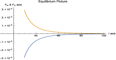
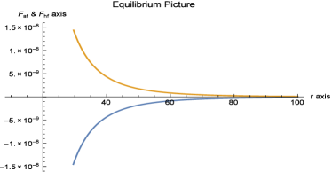
Figure 17: This shows the graphical illustration of $F_{af}$ and $F_{hf}$ forces versus $r$ for Gaussian and Lorentizian distribution when $f_{1}(R)=R$ in the left and right panels, respectively. Here, $\theta=0.5,M=0.01,n=3,\alpha=2.5,\gamma=2.5$ and $\lambda=2$

Similarly, we investigate the stability of numerical solutions for modified cubic $f(R)$ model using both the Gaussian and Lorentzian distributions. The graphical behavior of resulting forces is given by Figure 18. Its left part corresponds to behavior of these forces for Gaussian distribution whereas the right graph provides the behavior for Lorentzian distribution which clearly indicates that these forces are also balancing each other’s effect and thus leading to a stable wormhole structure.

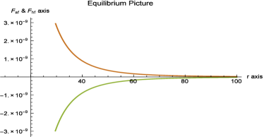
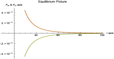
Figure 18: This shows the development of $F_{af}$ and $F_{hf}$ forces versus $r$ for Gaussian and Lorentzian distributions when $f(R)=R+\alpha R^{2}+\gamma R^{3}$. Here, we fix: $\theta=0.5,M=0.01,n=3,\alpha=2.5,\gamma=2.5$ and $\lambda=2$.

VI Gravitational Lensing effect of Wormhole for Simple $f(R)=R$ model

In this section, we will explore the possible detection of traversable wormhole through gravitational lensing phenomena. For this purpose, we consider the static spherical symmetric metric involving $x=\frac{r}{2M}$ representing the radius in Schwarzschild units and is given by

$$ds^{2}=-A(x)dt^{2}+B(x)dx^{2}+C(x)(d\theta^{2}+\sin^{2}\theta d\phi^{2}).$$ (34)

Here the closest path taken by the light ray is $\hat{x}=\frac{\hat{r}}{2M}$. Here we will consider the obtained exact form of shape function in case of simple linear $f_{1}(R)=R$ model (section III). The integration of this shape function from wormhole throat $r_{0}$ to $r$ is given as follows

$$b(r)=\frac{(\lambda+8\pi)M\sqrt{\theta}}{2\pi^{2}}[\frac{1}{\sqrt{\theta}}\arctan(\frac{r}{\sqrt{\theta}})-\frac{r}{(r^{2}+\theta)}-\frac{1}{\sqrt{\theta}}\arctan(\frac{r_{0}}{\sqrt{\theta}})-\frac{r_{0}}{(r_{0}^{2}+\theta)}]+r_{0}.$$ (35)

Here clearly the coupling constant satisfies $\lambda\neq-8\pi$. Basically, we consider the form of static spherically symmetric wormhole metric (5) where $e^{2\Phi(r)}=(\frac{r}{b_{0}})^{m}$ where $b_{0}$ is an integration constant while $m=2(v^{\phi})^{2}$, where $v^{\phi}$ indicates the rotational velocity. In 25 , it is pointed out that $m=0.000001$ which is very small values (nearly zero) and hence leaving the red shift function as a constant (as we assumed in previous sections). The comparison of these metrics leads to the following relations:

$$A(x)=(\frac{r}{b_{0}})^{m},\quad B(x)=(1-\frac{b(r)}{r})^{-1},\quad C(x)=r^{2}.$$ (36)

The deflection angle for light ray is given by

$$\alpha(\hat{x})=-\ln(\frac{2d}{3}-1)-0.8056+I(\hat{x}).$$ (37)

Here $d$ represents the mouth of wormhole because of exterior Schwarzschild line element while the internal metric contribution is provided by $I(\hat{x})$ which determines that the closest path taken by the ray of light is bigger than the wormhole mouth. This is defined by the relation:

$$I(\hat{x})=\int^{\infty}_{\hat{x}}\frac{2\sqrt{B(x)dx}}{\sqrt{C(x)\sqrt{\frac{C(x)A(\hat{x})}{C(\hat{x})A(x)}}-1}}.$$ (38)

In our case, this integral take the following form:

$$I(\hat{x})=\int^{d}_{\hat{x}}G(x)dx$$ (39)

representing the closest approach for the light ray to be inside the wormhole mouth. Here the function $G(x)$ is given by

$$G(x)=\frac{2}{\sqrt{x^{2}[1-\frac{1}{x}(\frac{\lambda+8\pi}{4\pi^{2}})(\arctan(\frac{x}{\sqrt{\theta}})-\frac{x\sqrt{\theta}}{(x^{2}+\theta)}-\arctan(\frac{x_{0}}{\sqrt{\theta}})+\frac{x_{0}\sqrt{\theta}}{(x^{2}_{0}+\theta)})+x_{0}]}\sqrt{\frac{x^{2-m}}{\hat{x}^{2-m}}-1}}.$$ (40)

In order to investigate the convergence/divergence of this integral, we can redefine the variable as $y=\frac{x}{\hat{x}}$ for the sake of simplicity in calculations. Thus the integral takes the following form

$$I(\hat{x})=\int^{d/\hat{x}}_{1}\frac{2}{\sqrt{[1-\frac{1}{\hat{x}y}(\frac{\lambda+8\pi}{4\pi^{2}})(\arctan(\frac{\hat{x}y}{\sqrt{\theta}})-\frac{\hat{x}y\sqrt{\theta}}{(\hat{x}^{2}y^{2}+\theta)}-\arctan(\frac{\hat{x}y_{0}}{\sqrt{\theta}})+\frac{\hat{x}y_{0}\sqrt{\theta}}{(\hat{x}^{2}y_{0}^{2}+\theta)})+\hat{x}y_{0}]}\sqrt{y^{4-m}-y^{2}}}.$$ (41)

In the integrand of the above integral, we can assume that $H(y)=f(y)(y^{4-m}-y^{2})$, where

$$f(y)=1-\frac{1}{\hat{x}y}(\frac{\lambda+8\pi}{4\pi^{2}})[\arctan(\frac{\hat{x}y}{\sqrt{\theta}})-\frac{\hat{x}y\sqrt{\theta}}{(\hat{x}^{2}y^{2}+\theta)}-\arctan(\frac{\hat{x}y_{0}}{\sqrt{\theta}})+\frac{\hat{x}y_{0}\sqrt{\theta}}{(\hat{x}^{2}y_{0}^{2}+\theta)}]+\hat{x}y_{0}.$$ (42)

Taylor’s series can be used to expand the function $H(y)$ around $y=1$ as follows

$$H(y)=(2-m)f(1)(y-1)+[\frac{1}{2}(5-m)(2-m)f(1)+(2-m)f^{\prime}(1)](y-1)^{2}+O(y-1)^{3}.$$ (43)

Here we truncate the Taylor’s expansion up to second-order where $O(y-1)^{3}$ indicates the cubic and higher-order terms of factor $(y-1)$. It can be easily observed that the integral $I(\hat{x})$ converges or diverges because of the leading term in the above expression. Integral can be convergent if the first $(y-1)^{1/2}$ leads the expression where $g(1)\neq 0$. If $g(1)=0$, then second term will lead the expression and whose integration will be $\ln(y-1)$. Since $y=1$, therefore it turns out be undefined there and hence the integral diverges. If we choose the nearest approach of light ray as the wormhole throat, i.e., $\hat{r}=r_{0}$, then consequently, we have $y_{0}=\frac{x_{0}}{\hat{x}}$ and thus $y_{0}=1$. Using these values in $f(y)$, it can be easily verified that $f(1)=0$. Hence a photon sphere with radius $\hat{r}$ (closest path taken by light ray) equal to throat radius $r_{0}$, can be found.

VII Conclusions

The existence and construction of wormhole solutions in GR with some exotic matter has always been of great interest for the researchers. The presence of exotic matter is one of the most important requirement for wormhole construction as it leads to NEC violation and hence permits the wormhole existence. In case of modified theories, construction of wormholes has become more fascinating topic as these include the effective energy-momentum tensor that violates NEC without inclusion of any exotic matter separately. In the present paper, we have constructed spherically symmetric wormhole solutions in the presence of two interesting Gaussian and Lorentzian distributions of non-commutative geometry in $f(R,T)$ modified gravity. For this purpose, in order to make system of equations closed, we assumed the function $f(R,T)=f_{1}(R)+\lambda T$ with two different forms of $f_{1}(R)$, i.e., the linear form $f_{1}(R)=R$ and $f_{1}(R)=R+\alpha R^{2}+\gamma R^{n},~{}n\geq 3$.

Firstly, we talked about the possible wormhole construction for the linear $f_{1}(R)$ model with both Gaussian and Lorentzian distributions. For Lorentzian and Gaussian distribution, we found the exact solution. In order to examine the physical behavior of these obtained solutions, we plotted $b(r)$ versus radial coordinate. It is observed that shape functions show positive increasing behaviors for both these non-commutative distributions. Further we found the location of wormhole throats and analyzed some important characteristics of the shape functions namely asymptotic behavior, the flaring out condition and the violation of NEC using graphs. This discussion has been given in Figures 1-8. It is concluded from these graphs that the obtained shape functions show asymptotic behavior, i.e., $\frac{b(r)}{r}\rightarrow 0$ as $r\rightarrow\infty$. Also, for both cases, wormhole throats are located at $r_{0}=0.2$ and $r_{0}=0.1$. Furthermore, the obtained shape functions are compatible with the flaring out condition and NEC as the function $\rho+p_{r}$ indicated negative behavior for both distributions. Thus the obtained solutions are viable permitting wormhole to exist in non-commutative $f(R,T)$ gravity.

Secondly, we checked the wormhole existence for model $f_{1}(R)=R+\alpha R^{2}+\gamma R^{n},~{}n\geq 3$ by taking both non-commutative distributions into account. In this case, we obtained very complicated non-linear differential equations for $b(r)$ whose analytic solutions are not possible, therefore we solved them numerically. It is worthwhile to mention here that we fixed $n=3$ for numerical solutions and their graphical behaviors as it is found that for $n>3$, the obtained solutions are not physically interesting (not meeting the necessary criteria for wormhole existence). In the left parts of Figure 9 and 13, it is shown that the numerical solutions for $b(r)$ indicate increasing positive behavior. Other necessary conditions like asymptotic behavior of shape function, flaring out condition as well as NEC have been given in Figures 9-16. The wormhole throat for solutions in both distributions are located at $r_{0}=0.001$. Also, $\rho+p_{r}$ shows negative behavior and hence NEC is incompatible for this solution. Thus it is concluded that all the conditions are satisfied for the chosen specific values of free parameters and hence the obtained wormhole solutions are viable. It is also interesting to mention here that for a different selection of free parameters $\theta,~{}M,~{}\lambda$ etc. (other than the used values in the present paper), all the functions show a similar graphical behavior as presented in the Figures. Thus all the necessary conditions for wormhole existence will also be satisfied in these cases and hence the wormhole solution still exist.

Further, we examined the stability of obtained solutions using equilibrium condition given by Tolman-Oppenheimer-Volkov equation. Here we explored the stability for both models of $f_{1}(R)$ in the presence of Gaussian and Lorentzian distributions. After evaluating the possible expressions of anisotropic and hydrostatic forces for these cases, we examined them graphically as shown in Figures 17 and 18. It can be easily observed from the graphs that these forces are almost equal in magnitude but opposite in behavior, therefore canceling each other’s effect and hence leaving a balanced final wormhole configuration. Furthermore, we explored the possible detection of photon sphere at wormhole throat. For this purpose, we followed the procedure given in reference 25 and explored the convergence of deflection angle. It is observed that for the obtained exact solution for $f_{1}(R)=R$, the resulting integral diverges at wormhole throat and hence it is concluded that a photon sphere with radius $r_{0}$ (closest path taken by light ray) equal to throat radius, can be detected.

References

- (1) Perlmutter, S. et al.: Astrophys, J. 483(1997)565.
- (2) Perlmutter, S. et al.: Nature 391(1998)51.
- (3) Perlmutter, S. et al.: Astrophys, J. 517(1999)565.
- (4) Weinberg, S.: Rev. Mod. Phys. 61(1989)1.
- (5) Bento, M.C., Bertolami, O. and Sen, A.A.: Phys. Rev. D 66(2002)043507; Fujii, Y.: Phys. Rev. D 26(1982)2580; Ford, L.H.: Phys. Rev. D 35(1987)2339; Wetterich, C.: Nucl. Phys. B 302(1988)668; Ratra, B. and Peebles, P.J.E.: Phys. Rev. D 37(1988)3406; Chiba, T., Sugiyama, N. and Nakamura, T.: Mon. Not. Roy. Astron. Soc. 289(1997)L5; Caldwell, R.R., Dave, R. and Steinhardt, P.J.: Phys. Rev. Lett. 80(1998)1582; Armendariz-Picon, C., Damour, T. and Mukhanov, V.F.: Phys. Lett. B 458(1999)209; Chiba, T., Okabe, T. and Yamaguchi, M.: Phys. Rev. D 62(2000)023511, Chimento, L.P.: Phys. Rev. D 69(2004)123517; Chimento, L.P. and Feinstein, A.: Mod. Phys. Lett. A 19(2004)761.
- (6) Nojiri, S. and Oditsov, S.D.: Phys. Rep. 505(2011)59.
- (7) Starobinksy, A. A.: Phys. Lett. B 91(1980)99; Ferraro, R. and Fiorini, F.: Phys. Rev. D 75(2007)084031; Zubair, M.: Int. J. Modern. Phys. D 25(2016)1650057; Carroll, S. et al., Phys. Rev. D 71, 063513 (2005); Cognola, G.: Phys. Rev. D 73(2006)084007; Agnese, A. G. and Camera, M. La.: Phys. Rev. D 51(1995)2011; Kofinas, G. and Saridakis, N. E.: Phys. Rev. D 90(2014)084044; Sharif, M. and Waheed, S.: Adv. High Energy Phys. 2013(2013)253985; Zubair, M. and Kousar, F.: Eur. Phys. J. C (2016) 76:254; Zubair, M., Kousar, F. and Bahamonde, S.: Physics of the Dark Universe 14(2016)116 125.
- (8) Harko, T. et al.: Phys. Rev. D 84(2011)024020.
- (9) Houndjo, M. J. S. et al.: Int. J. Mod. Phys. D 21(2012)1250003; Sharif, M. and Zubair, M.: Gen. Relativ. Gravit. 46(2014)1723; Zubair, M. and Syed M. Ali Hassan: Astrophys Space Sci (2016) 361:149; Zubair, M., Syed M. Ali Hassan and Abbas, G.: Canadian Journal of Physics, 2016, 94(12): 1289-1296; Jamil, M., Momeni1, D, Raza, M. and Myrzakulov, R.: Eur. Phys. J. C 72(2012)1999.
- (10) Singh, C.P. and Singh, V.: Gen. Relativ. Gravitt. 46(2014)1696; Sharif, M. and Zubair, M.: J. Phys. Soc. Jpn. 82(2013)064001; Shabani, H. and Farhoudi, M.: Phys. Rev. D 88(2013)044048; ibid. Phys. Rev. D 90(2014)044031; Santos, A.F.: Modern Phys. Lett. A 28(2013)1350141; Zubair, M. and Noureen, I.: Eur. Phys. J. C 75(2015)265; Noureen, I. and Zubair, M.: Eur. Phys. J. C 75(2015)62; Noureen, I. and Zubair, M., Bhatti, A.A. and Abbas, G.: Eur. Phys. J. C 75(2015)323; Alvarenga et al.: Phys. Rev. D 87(2013)103526; Baffou et al. Astrophys. Space Sci. 356(2015)173; Shamir, M.F.: Eur. Phys. J. C 75(2015)354; Moraes, P.H.R.S.: Eur. Phys. J. C 75(2015)168; Zubair, M. et al.: Astrophys Space Sci. 361(2016)8; Zubair, M., Azmat, H. and Noureen, I.: Eur. Phys. J. C (2017) 77:169; Shabani, H., and Farhoudi, M.: ibid. Phys. Rev. D 90, 044031 (2014).
- (11) Jamil, M., Momeni, D. and Myrzakulov, R.: Eur. Phys. J. C 73(2013)2267.
- (12) Einstein, A. and Rosen, N.: Phys. Rev. 48(1935)73.
- (13) Morris, M. S. and Thorne, K. S.: Am. J. Phys. 56(1988)395.
- (14) Kim, S. W. and Lee, H.: Phys. Rev. D 63(2001)064014; Jamil, M. and Farooq, M. U.: Int. J. Theor. Phys. 49(2010)835; Rahaman, F. and Islam, S., Kuhfittig, P. K. F. and Ray, S.: Phys. Rev. D 86(2012)106010; Lobo, F.S.N., Parsaei, F. and Riazi, N.: Phys. Rev. D 87(2013)084030; Rahaman, F. et al.: Int. J. Theor. Phys. 53(2014)1910; Sharif, M. and Rani, S.: Eur. Phy. J. Plus 129(2014)237; Jamil, M. et al.: J. Korean Phys. Soc. 65(2014)917; Zubair, M., Waheed, S. and Ahmad, Y.: Eur. Phys. J. C (2016) 76:444.
- (15) Khufittig, P. K. F.: Eur. Phys. J. C 74(2014)2818.
- (16) Kanti, P., Kleihaus, B. and Kunz, J.: Phys. Rev. Lett. 107(2011)271101; Phys. Rev. D 85(2012)044007.
- (17) Moraes, P., Correa, R. and Lobato, R.: JCAP 07(2017)1707.
- (18) Witten, E.: Nucl. Phys. B 460(1996)335; Seiberg, N. and Witten, E.: J. High Energy Phys. 09 (1999).
- (19) Gruppuso, A.: J. Phys. A 38(2005)2039; Smailagic, A. and Spalluci, E. : J. Phys. A 36(2003)467L; Nicolini, P., Smailagic, A. and Spalluci, E.: Phys. Lett. B 632(2006)547.
- (20) Sushkov, S. V.: Phys. Rev. D 71 (2005) 043520.
- (21) Nicolini, P. and Spalluci, E.: Classical Quantum Gravity 27, 015010 (2010).
- (22) Morris, M.S., Throne, K.S. and Yurtseve, U.: Phys. Rev. Lett. 61, 1446 (1988).
- (23) Moraes, P.H.R.S.: Astrophys. Space Sci. 352(2014); Eur. Phys. J. C 75(2015)168.
- (24) Ozkan, M. and Pang, Y.: Class. Quantum Grav. 31(2014)205004.
- (25) Goswami, U.D. and Deka, K.: Int. J. Mod. phys. D 22(2013)1350083.
- (26) Tejeiro, J. M. and Larranaga, E. A.: arXiv: gr-qc/0505054; Rom. J. Phys. 57(2012)736; Kuhfittig, P.K.F.: Eur. Phys. J. C 74(2014)2818; Scientific Voyage 2(2016)1.