Optimized Structured Sparse Sensing Matrices for Compressive Sensing

Abstract

We consider designing a robust structured sparse sensing matrix consisting of a sparse matrix with a few non-zero entries per row and a dense base matrix for capturing signals efficiently. We design the robust structured sparse sensing matrix through minimizing the distance between the Gram matrix of the equivalent dictionary and the target Gram of matrix holding small mutual coherence. Moreover, a regularization is added to enforce the robustness of the optimized structured sparse sensing matrix to the sparse representation error (SRE) of signals of interests. An alternating minimization algorithm with global sequence convergence is proposed for solving the corresponding optimization problem. Numerical experiments on synthetic data and natural images show that the obtained structured sensing matrix results in a higher signal reconstruction than a random dense sensing matrix.

1 Introduction

Compressive sensing (CS) supplies a paradigm of joint compression and sensing signals of interest [1, 2]. A CS system contains two main ingredients: a sensing matrix $\bar{\bm{\Phi}}\in\mathbb{R}^{M\times N}$ ($M\ll N$) which compresses a signal $\bm{x}$ via $\bm{y}=\bar{\bm{\Phi}}\bm{x}$ and a dictionary $\bar{\bm{\Psi}}\in\mathbb{R}^{N\times L}$ ($L\geq N$) that captures the sparse structure of the signal. In particular, we say $\bm{x}\in\mathbb{R}^{N}$ is sparse if it can be represented with a few columns of $\bar{\bm{\Psi}}$:

$$\bm{x}=\bar{\bm{\Psi}}\bm{s}+\bm{e}=\sum_{\ell}\bar{\bm{\Psi}}(:,\ell)\bm{s}(\ell)+\bm{e},$$ (1)

where $\|\bm{s}\|_{0}\leq K$ with $K\ll N\leq L$. The term $\bm{e}$ is referred to as the sparse representation error (SRE) of $\bm{x}$ under $\bar{\bm{\Psi}}$. If $\bm{e}$ is nil, we say $\bm{x}$ is exactly sparse.

The choice of dictionary $\bar{\bm{\Psi}}$ depends on the signal model and traditionally it is chosen to concisely capture the structure of the signals of interest, e.g., the Fourier matrix for frequency-sparse signals, and a multiband modulated Discrete Prolate Spheroidal Sequences (DPSS’s) dictionary for sampled multiband signals [3]. Furthermore, we can also learn a dictionary from a set of representative signals (training data) called dictionary learning [4, 5, 6].

In CS, the sensing matrix $\bar{\bm{\Phi}}$ is used to preserve the useful information contained in the signal $\bm{x}$ such that it is possible to recover $\bm{x}$ from its low dimensional measurements $\bm{y}=\bar{\bm{\Phi}}\bm{x}$. It has been shown that if the equivalent dictionary $\bar{\bm{\Phi}}\bar{\bm{\Psi}}$ satisfies the restricted isometry property (RIP), the sparse vector $\bm{s}$ in (1) can be exactly recovered from $\bm{y}$ [7, 1]. Although random matrices satisfy the RIP with high probability [7], confirming whether a general matrix satisfies the RIP is NP-hard [8]. Alternatively, mutual coherence, another measure of sensing matrices that is much easier to verify, has been introduced in practice to quantify and design sensing matrices [9, 10, 11, 12, 13, 14, 15, 16, 17, 18, 19].

Structured sensing matrices (e.g., Toeplitz matrices and sparse matrices) have been proposed [20, 21, 22, 23, 24, 25, 26] to reduce the computational complexity of sensing signals in hardware (such as digital signal processor and FPGA) [27, 28], or applications like electrocardiography (ECG) compression [29] and data stream computing [30]. A Toeplitz matrix can be implemented efficiently to a vector by the fast Fourier transform (FFT). The advantage of sparse sensing matrix over a regular one is that it contains fewer non-zero elements per row and thus can significantly reduce the number of multiplication units for practical applications. However, similar to a random sensing matrix, a random sparse one is less competitive than an optimized sensing matrix regarding signal recovery accuracy.

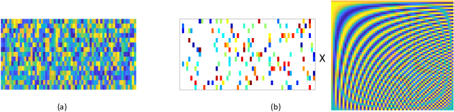
Figure 1: (a) a random Gaussian matrix; (b) a structured sparse sensing matrix consists of a sparse sensing matrix and a base sensing matrix

Motivated by this, we consider the design of a structured sparse sensing matrix that can not only efficiently compress signals but also has similar performance as the dense ones. Specifically, we attempt to design a structured sparse sensing matrix via enhancing the mutual coherence (defined in (2)) property of the equivalent dictionary, $\bar{\bm{\Phi}}\bar{\bm{\Psi}}$. Our main contributions are stated as follows:

• We propose a framework for designing a structured sparse sensing matrix by decreasing the mutual coherence of the equivalent dictionary. As shown in Figure 1, the structured sparse sensing matrix consists of $\widetilde{\bm{\Phi}}\bm{A}$ where $\widetilde{\bm{\Phi}}\in\mathbb{R}^{M\times N}$ is a row-wise sparse matrix while $\bm{A}\in\mathbb{R}^{N\times N}$ is referred to a base sensing matrix that can be implemented with linear complexity to a signal. In general, the choice of $\bm{A}$ depends on the practical situations, e.g., we choose $\bm{A}$ as a DCT matrix when used for natural images with a dictionary learned by the KSVD algorithm [5]. For some cases, one may simply set $\bm{A}$ as an identity matrix, giving a sparse sensing matrix. To our knowledge, this work is the first attempt to optimize a (structured) sparse sensing matrix by minimizing the mutual coherence.

• We provide an alternating minimization algorithm for solving the formulated nonconvex nonsmooth optimization problem (see (11)). Despite the nonconvexity and nonsmoothness, we perform a rigorous convergence analysis to show that the sequence of iterates generated by our proposed algorithm with random initialization converges to a critical point.

• Experiments on natural images show that the obtained structured sensing matrix—with or without $\bm{A}$—outperforms a random dense sensing matrix. It is of interest to note that by setting $\bm{A}$ as the DCT matrix, the optimized structured sensing matrix has almost identical performance in terms of Peak Signal to Noise Ratio (PSNR) as the optimized dense sensing matrix, see Figure 8.

The outline of this paper is given as follows. We review the previous approaches in robust sensing matrix design in Section 2. In Section 3, a framework for designing a structured sparse sensing matrix is proposed with the mutual coherence behavior of the equivalent dictionary and the SREs of the signals being considered simultaneously. An alternating minimization algorithm for solving the optimal design problem with a rigorous convergence analysis is provided in Section 4. We validate the performance of the obtained structured sensing matrix on both synthetic data and real images in Section 5. Conclusions are given in Section 6.

2 Preliminaries

In this section, we will brief the definition of mutual coherence to CS and introduce the previous work on designing robust sensing matrices.

2.1 Mutual Coherence

The mutual coherence of $\bm{Q}\in\mathbb{R}^{M\times L}$ is defined as

$$\mu(\bm{Q})\triangleq\max_{1\leq i\neq j\leq L}\frac{|\bm{q}_{i}^{\cal T}\bm{q}_{j}|}{\|\bm{q}_{i}\|_{2}\|\bm{q}_{j}\|_{2}}\geq\underline{\mu}\triangleq\sqrt{\frac{L-M}{M(L-1)}},$$ (2)

where $\bm{q}_{i}$ is the $i$th column of $\bm{Q}$ and $\underline{\mu}$ is the lower bound of $\mu(\bm{Q})$ called Welch Bound [31]. The connection between the mutual coherence and the RIP is given in [32, Section 5.2.3]. Roughly speaking, the smaller mutual coherence, the better the RIP.

With the measurements $\bm{y}=\bar{\bm{\Phi}}\bm{x}$ and the prior information that $\bm{x}$ is sparse in $\bar{\bm{\Psi}}$, we can recover the signal as $\widehat{\bm{x}}=\bar{\bm{\Psi}}\widehat{\bm{s}}$ where

$$\widehat{\bm{s}}=\mathop{\rm argmin}_{\bm{s}}\leavevmode\nobreak\ \|\bm{y}-\bar{\bm{\Phi}}\bar{\bm{\Psi}}\bm{s}\|_{2}^{2}\leavevmode\nobreak\ \leavevmode\nobreak\ \leavevmode\nobreak\ \leavevmode\nobreak\ \text{s.t.}\leavevmode\nobreak\ \leavevmode\nobreak\ \leavevmode\nobreak\ \|\bm{s}\|_{0}\leq K$$ (3)

which can be exactly or approximately solved via convex methods [1, 33, 34] or greedy algorithm [35], e.g., the orthogonal marching pursuit (OMP). It is shown in [35] that OMP can stably find $\bm{s}$ (and hence obtain an accurate estimation of $\bm{x}$) if

$$K<\frac{1}{2}\left[1+\frac{1}{\mu(\bar{\bm{\Phi}}\bar{\bm{\Psi}})}\right].$$ (4)

2.2 Optimized Robust Sensing Matrix [14, 16]

Motivated by (4), abundant efforts have been devoted to design the sensing matrix via minimizing the mutual coherence $\mu(\bar{\bm{\Phi}}\bar{\bm{\Psi}})$, including a subgradient projection method [36], and the ones based on alternating minimization. [9, 11, 12]. Experiments on synthetic data indicate that the obtained sensing matrices give much better performance than the random one when the signals are exactly sparse, i.e., $\bm{e}=\bm{0}$ in (1).

However, it was recently realized that an optimized sensing matrix obtained by minimizing the mutual coherence is not robust to SRE in (1) and thus the corresponding CS system yields poor performance [14]. In particular, the SRE always exists in the practical signals of interests, even representing them via a learned dictionary [5]. Let $\bm{X}\in\mathbb{R}^{N\times J}$ be a set of training data and $\bm{S}$ consist of the sparse coefficients of $\bm{X}$ in $\bar{\bm{\Psi}}$: $\bm{X}=\bar{\bm{\Psi}}\bm{S}+\bm{E}$ where $\|\bm{S}(:,j)\|_{0}\leq K,\forall j$. Then, in [14, 16], the SRE matrix

$$\bm{E}:=\bm{X}-\bar{\bm{\Psi}}\bm{S}$$ (5)

is utilized as the regularization to yield a robust sensing matrix.

Denote by $\mathcal{G}_{\xi}$ the set of relaxed equiangular tight frame (ETF) Gram matrices:

$$\mathcal{G}_{\xi}=\bigg{\{}\bm{G}\in\mathbb{S}^{L\times L}:\bm{G}(i,i)=1,\forall i,\max_{i\neq j}|\bm{G}(i,j)|\leq\xi\bigg{\}},$$ (6)

where $\xi\in[0,1)$ is a pre-set threshold and usually chosen as $0$ or $\underline{\mu}$ [11, 12, 14, 16] and $\mathbb{S}^{L\times L}$ denotes a set of real $L\times L$ symmetric matrices. Then the sensing matrices proposed in [14, 16] are optimized by solving the following optimization problem:

$$\underset{\bar{\bm{\Phi}},\bm{G}\in\mathcal{G}_{\xi}}{\text{min}}\leavevmode\nobreak\ ||\bm{G}-\bar{\bm{\Psi}}^{\mathrm{T}}\bar{\bm{\Phi}}^{\mathrm{T}}\bar{\bm{\Phi}}\bar{\bm{\Psi}}||^{2}_{F}+\lambda\|\bar{\bm{\Phi}}\bm{E}\|_{F}^{2},$$ (7)

where the first term is utilized to control the average mutual coherence of the equivalent dictionary, the second term $\|\bar{\bm{\Phi}}\bm{E}\|_{F}^{2}$ is a regularization to make the sensing matrix robust to SRE, and $\lambda\geq 0$ is the trade-off parameter to balance these two terms. Compared with previous work, simulations have shown that the obtained sensing matrices by (7) achieve the highest signal recovery accuracy when the SRE exists [14].

3 Optimized Structured Sparse Sensing Matrix

In this section, we consider designing a structured sensing matrix by taking into account the complexity of signal sensing procedure, robustness against the SRE and the mutual coherence of the equivalent dictionary simultaneously.

As mentioned above, in applications like ECG compression [29], data stream computing [30] and hardware implementation [27], the classical CS system with a dense sensing matrix $\bar{\bm{\Phi}}$ encounters computational issues. Indeed, merely applying a sensing matrix $\bar{\bm{\Phi}}\in\mathbb{R}^{M\times N}$ to capture a length-$N$ signal has the computational complexity of $\mathcal{O}(MN)$. Moreover, in applications like image processing, one often partitions the image into a set of patches of small size (say $8\times 8$ patches, hence $N=64$) to make the problem computationally tractable. However, the recent work in dictionary learning [37] and sensing matrix design [17] has revealed that larger-size patches (say $64\times 64$ patches, hence $N=4096$) lead to better performance for image processing like image denoising and compression. All of these enforce us to reduce the complexity of sensing a signal.

An approach to tackle this computational difficulties is to impose certain structures into the sensing matrix $\bar{\bm{\Phi}}$. One of such structures is the sensing matrix consisting of a sparse matrix and a base matrix that both can be efficiently implemented to sensing signals:

$$\bar{\bm{\Phi}}=\widetilde{\bm{\Phi}}\bm{A},$$ (8)

where $\bm{A}\in\mathbb{R}^{N\times N}$ is referred to as a base sensing matrix and $\widetilde{\bm{\Phi}}\in\mathbb{R}^{M\times N}$ is a row-wise sparse matrix.

To maintain the original purpose for reducing sensing complexity of $\bm{y}=\bar{\Phi}\bm{x}$, we restrict the choices of the base sensing matrix $\bm{A}$ to be either identity matrix or the one that admits fast multiplications like DCT matrix. We also note that the choice of base sensing matrix $\bm{A}$ should depend on specific applications, e.g., we can set $\bm{A}$ to be a DCT matrix in image processing task [38]. Rewrite (8) as

$$\bar{\bm{\Phi}}^{\mathrm{T}}=\bm{A}^{\mathrm{T}}\widetilde{\bm{\Phi}}^{\mathrm{T}}$$ (9)

and view $\widetilde{\bm{\Phi}}^{\mathrm{T}}$ as the sparse representation of $\bar{\bm{\Phi}}^{\mathrm{T}}$ in $\bm{A}^{\mathrm{T}}$. Thus, similar to (1) where we call $\bm{x}$ is sparse (in $\bar{\bm{\Psi}}$) though itself is not sparse, we also say that $\bar{\bm{\Phi}}$ in (8) is a sparse sensing matrix (in $\bm{A}$). Note that the structure of (9) also appears in the double-sparsity dictionary learning task [38], the dictionary $\bar{\bm{\Psi}}=\bm{A}\widetilde{\bm{\Psi}}$ with $\widetilde{\bm{\Psi}}$ being overcomplete but column-wise sparse.

Note that the approach shown in [14, 16] requires the explicit formulation of the SRE matrix $\bm{E}$ (defined in (5)) which can be huge or need extra effort to obtain in some applications, like image processing with a wavelet dictionary that no typical training data is available [17]. Let us draw each column of $\bm{E}$ from an independently and identically distributed (i.i.d.) Gaussian distribution of mean zero and covariance $\sigma^{2}{\bf I}$. Then $\frac{\|\bar{\bm{\Phi}}\bm{E}\|_{F}^{2}}{J}$ converges in probability and almost surely to $\sigma^{2}\|\bar{\bm{\Phi}}\|_{F}^{2}$ when the number of training samples $J$ approaches to $\infty$ [17]. Thus we can get rid of the SRE matrix $\bm{E}$ by minimizing $\|\bar{\bm{\Phi}}\|_{F}$ directly to yield a sensing matrix that is robust to the SRE.

Now our goal is to find a structured sensing matrix $\bar{\bm{\Phi}}=\widetilde{\bm{\Phi}}\bm{A}$ such that it is robust to the SRE of the signals and the equivalent dictionary $\bar{\bm{\Phi}}\bar{\bm{\Psi}}$ has a small mutual coherence. So the corresponding sparse matrix is obtained via solving

$$\{\widetilde{\bm{\Phi}},\widetilde{\bm{G}}\}= \mathop{\rm argmin}_{\bm{\Phi},\bm{G}\in\mathcal{G}_{\xi}}||\bm{G}-\bar{\bm{\Psi}}^{\mathrm{T}}\bm{A}^{\mathrm{T}}\bm{\Phi}^{\mathrm{T}}\bm{\Phi}\bm{A}\bar{\bm{\Psi}}||^{2}_{F}+\lambda\|\bm{\Phi}\bm{A}\|_{F}^{2}$$

$$\leavevmode\nobreak\ \leavevmode\nobreak\ \leavevmode\nobreak\ \leavevmode\nobreak\ \leavevmode\nobreak\ \text{s.t.}\leavevmode\nobreak\ \leavevmode\nobreak\ \leavevmode\nobreak\ \|\bm{\Phi}(m,:)\|_{0}\leq\kappa,\ \forall\ m,$$ (10)

where $\kappa$ denotes the number of non-zero elements in each row of the sensing matrix.

Without the base matrix $\bm{A}$, the complexity of $\bar{\bm{\Phi}}\bm{x}=\widetilde{\bm{\Phi}}\bm{x}$ is $O(M\kappa)$ which is the same as the one shown in [23]. Thus, there is a tradeoff in adding the base matrix $\bm{A}$ since the base matrix may improve the performance, but also increase the computational complexity. Fortunately, by choosing as a DCT matrix, it only slightly increase the computation of $O(N\log N)$ which is small or comparable to $O(M\kappa)$. Moreover, in some cases, $\bm{A}\bm{x}$ can be implemented with complexity $O(N)$. For example, if $\bm{A}$ is an orthogonal matrix and we decompose it into a series of Givens rotation matrices [39]. This is a significant reduction of computational complexity compared with a dense sensing matrix requiring a complexity of $O(MN)$ to sense a signal when $N$ is large and $N\gg\kappa$. We show the difference between $O(MN)$ and $O(N\log N+M\kappa)$ in Figure 2 with various $\kappa$ and $N$.

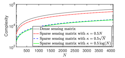
Figure 2: Illustration of the complexity $O(MN)$ (the dotted black line) and $O(N\log N+M\kappa)$ (the other three lines indicating different $\kappa$) with $M=10\log N$.

4 Proposed Algorithm for Designing Structured Sensing Matrix

Aside from the facts that $\bar{\bm{\Phi}}$ is parameterized by $\widetilde{\bm{\Phi}}\bm{A}$ and $\|\bar{\bm{\Phi}}\bm{E}\|_{F}^{2}$ is replaced by $\|\bar{\bm{\Phi}}\|_{F}^{2}$, (10) differs from (7) in that the former has a sparse constraint on the rows of $\widetilde{\bm{\Phi}}$. Note that such a constraint makes (10) highly nonconvex. In this section, we suggest utilizing alternating projected gradient method to address (10). Moreover, we also provide a rigorous convergence analysis of the proposed algorithm.

4.1 Proposed Algorithm for Designing Structured Sensing Matrix

Assume $\bm{A}$ is not null and rewrite (10) as

$$\begin{split}&\min_{\bm{\Phi},\bm{G}}f(\bm{\Phi},\bm{G})=||\bm{G}-\bm{\Psi}^{\mathrm{T}}\bm{\Phi}^{\mathrm{T}}\bm{\Phi}\bm{\Psi}||^{2}_{F}+\lambda\|\bm{\Phi}\|_{F}^{2}\\ &\leavevmode\nobreak\ \leavevmode\nobreak\ \leavevmode\nobreak\ \text{s.t.}\leavevmode\nobreak\ \leavevmode\nobreak\ \|\bm{\Phi}(m,:)\|_{0}\leq\kappa,\ \forall\ m,\ \bm{G}\in\mathcal{G}_{\xi}\end{split}$$ (11)

where $\bm{\Psi}=\bm{A}\bar{\bm{\Psi}}$. Let $\mathcal{P}_{\mathcal{G}_{\xi}}:\mathbb{R}^{L\times L}\rightarrow\mathbb{R}^{L\times L}$ denote an orthogonal projector onto the set $\mathcal{G}_{\xi}$:

$$\left(\mathcal{P}_{\mathcal{G}_{\xi}}(\bm{G})\right)(i,j)=\left\{\begin{matrix}1,&i=j,\\ \operatorname{sign}(\bm{G}(i,j))\min(|\bm{G}(i,j)|,\xi),&i\neq j,\end{matrix}\right.$$

where $\operatorname{sign}(\cdot)$ denotes the sign function. Firstly the solution of minimizing $f$ in terms of $\bm{G}$ with fixed $\bm{\Phi}$ is given by

$$\widehat{\bm{G}}=\mathop{\rm argmin}_{\bm{G}\in\mathcal{G}_{\xi}}f(\bm{\Phi},\bm{G})=\mathcal{P}_{\mathcal{G}_{\xi}}(\bm{\Psi}^{\mathrm{T}}\bm{\Phi}^{\mathrm{T}}\bm{\Phi}\bm{\Psi}).$$ (12)

Now we consider solving (11) in terms of $\bm{\Phi}$ with fixed $\bm{G}$:

$$\min_{\bm{\Phi}}f(\bm{\Phi},\bm{G})\leavevmode\nobreak\ \leavevmode\nobreak\ \leavevmode\nobreak\ \text{s.t.}\ \|\bm{\Phi}(m,:)\|_{0}\leq\kappa,\ \forall\ m.$$ (13)

Without the sparsity constraint, the recent works [40, 41] have shown that any gradient-based algorithms can provably solve $\min_{\bm{\Phi}}f(\bm{\Phi},\bm{G})$. Thus, we suggest utilizing the projected gradient descent (PGD) to solve (13) with the sparsity constraint. The gradient of $f(\bm{\Phi},\bm{G})$ with respect to $\bm{\Phi}$ is:

$$\nabla_{\bm{\Phi}}f(\bm{\Phi},\bm{G})=2\lambda\bm{\Phi}-4\bm{\Phi}\bm{\Psi}\bm{G}\bm{\Psi}^{\mathrm{T}}+4\bm{\Phi}\bm{\Psi}\bm{\Psi}^{\mathrm{T}}\bm{\Phi}^{\mathrm{T}}\bm{\Phi}\bm{\Psi}\bm{\Psi}^{\mathrm{T}}.$$ (14)

For convenience, let $\mathcal{S}_{\kappa}$ denote the set of matrices which have at most $\kappa$ non-zero elements in each row:

$$\mathcal{S}_{\kappa}\triangleq\left\{\bm{Z}\in\mathbb{R}^{M\times N}:\|\bm{Z}(m,:)\|_{0}\leq\kappa,\ \forall\ m\right\}.$$

Denote $\mathcal{P}_{\cal S_{\kappa}}:\mathbb{R}^{M\times N}\rightarrow\mathbb{R}^{M\times N}$ as an orthogonal projector on the set of $\mathcal{S}_{\kappa}$: for any $M\times N$ input matrix, that keeps the largest $\kappa$ absolute values of each row. So, in the $k$th step, we update $\bm{\Phi}$ as

$$\bm{\Phi}_{k}\in\mathcal{P}_{\mathcal{S}_{\kappa}}\left(\bm{\Phi}_{k-1}-\eta\nabla f(\bm{\Phi}_{k-1},\bm{G}_{k-1})\right).$$ (15)

we choose an arbitrary one if there exist more than one projections.

We summarize the proposed alternating minimization for solving (11) in Algorithm 1. Note that alternating minimization-based algorithm has been popularly utilized for designing sensing matrix [9, 10, 11, 12, 14, 16]. However, the convergence of these algorithms is usually neither ensured nor seriously considered. In the following, we provide the rigorous convergence analysis of the proposed Algorithm 1.

Algorithm 1 Algorithm for Designing Sparse Sensing Matrix

0:   Initial value $\bm{\Phi}_{0}$, the number of maximal iterations $Iter_{max}$, step size $\eta$, the sparsity level $\kappa$ and the given trade-off parameter $\lambda$.

0:   Sparse sensing matrix $\bm{\Phi}_{Iter_{max}}$.

1:  $k\leftarrow 1$

2:  while $k\leq Iter_{max}$ do

3:     Update $\bm{\Phi}$: $\bm{\Phi}_{k}\in\mathcal{P}_{\mathcal{S}_{\kappa}}(\bm{\Phi}_{k-1}-\eta\nabla_{\bm{\Phi}}f(\bm{\Phi}_{k-1},\bm{G}_{k-1}))$

4:     Update $\bm{G}$: $\bm{G}_{k}=\mathcal{P}_{\mathcal{G}_{\xi}}(\bm{\Psi}^{\mathrm{T}}\bm{\Phi}_{k}^{\mathrm{T}}\bm{\Phi}_{k}\bm{\Psi})$

5:     $k\leftarrow k+1$

6:  end while

4.2 Convergence Analysis

Transfer (11) into the following unconstrained problem

$$\begin{split}\min_{\bm{\Phi},\bm{G}}\rho(\bm{\Phi},\bm{G}):=f(\bm{\Phi},\bm{G})+\delta_{\mathcal{S}_{\kappa}}(\bm{\Phi})+\delta_{\mathcal{G}_{\xi}}(\bm{G}),\end{split}$$ (16)

where $\delta_{\mathcal{S}_{\kappa}}(\bm{\Phi})=\begin{cases}0,&\bm{\Phi}\in\mathcal{S}_{\kappa},\\ \infty,&\bm{\Phi}\notin\mathcal{S}_{\kappa}\end{cases}$ is the indicator function (and similarly for $\delta_{\mathcal{G}_{\xi}}(\bm{G})$). Clearly, (16) is equivalent to the original constrained problem (11). Compared with (11), it is easier to take the subdifferential for (16) since it has no constraints. Thus, in the sequel, we focus on (16) since the convergence analysis mainly involves the subdifferential.

Note that by updating $\bm{G}$ with (12), $\rho(\bm{\Phi}_{k},\bm{G}_{k})\leq\rho(\bm{\Phi}_{k},\bm{G}_{k-1})$. Following, we show the objective function is decreasing by updating the sensing matrix $\bm{\Phi}$. Denote $\rho_{0}=\rho(\bm{\Phi}_{0},\bm{G}_{0})$ and consider the sublevel set of $\rho$:

$$\mathcal{L}_{\rho_{0}}=\left\{(\bm{\Phi},\bm{G}):\rho(\bm{\Phi},\bm{G})\leq\rho_{0},\bm{G}\in\mathcal{G}_{\xi},\bm{\Phi}\in\mathcal{S}_{\kappa}\right\}.$$

It is clear that for any point $(\bm{\Phi},\bm{G})\in\mathcal{L}_{\rho_{0}}$, $\|\bm{G}\|_{F}$ is finite since $\bm{G}\in\mathcal{G}_{\xi}$ and $\|\bm{\Phi}\|_{F}$ is finite since $\rho\rightarrow\infty$ when $\|\bm{\Phi}\|_{F}\rightarrow\infty$. Then with simple calculation, we have that both $\nabla_{\bm{\Phi}}f(\bm{\Phi},\bm{G})$ and $\nabla_{\bm{G}}f(\bm{\Phi},\bm{G})$ are Lipshitz continuous,

$$\begin{split}&\|\nabla_{\bm{\Phi}}f(\bm{\Phi},\bm{G})-\nabla_{\bm{\Phi}}f(\bm{\Phi}^{\prime},\bm{G})\|_{F}\leq L_{c}\|\bm{\Phi}-\bm{\Phi}^{\prime}\|_{F}\\ &\|\nabla_{\bm{G}}f(\bm{\Phi},\bm{G})-\nabla_{\bm{G}}f(\bm{\Phi},\bm{G}^{\prime})\|_{F}\leq L_{c}\|\bm{G}-\bm{G}^{\prime}\|_{F}\end{split}$$ (17)

for all $(\bm{\Phi},\bm{G}),(\bm{\Phi}^{\prime},\bm{G}),(\bm{\Phi},\bm{G}^{\prime})\in\mathcal{L}_{\rho_{0}}$. Here $L_{c}>0$ is the corresponding Lipschitz constant. A direct consequence of the Lipschitz continuous is as follows.

Lemma 1.

For any $L\geq L_{c}$, denote by

$$h_{L}(\bm{\Phi},\bm{\Phi}^{\prime},\bm{G}):= f(\bm{\Phi}^{\prime},\bm{G})+\langle\nabla_{\bm{\Phi}}f(\bm{\Phi}^{\prime},\bm{G}),\bm{\Phi}-\bm{\Phi}^{\prime}\rangle$$

$$+\frac{L}{2}\|\bm{\Phi}-\bm{\Phi}^{\prime}\|_{F}^{2}.$$

Then, $f(\bm{\Phi},\bm{G})\leq h_{L}(\bm{\Phi},\bm{\Phi}^{\prime},\bm{G})$ for all $(\bm{\Phi},\bm{G}),(\bm{\Phi}^{\prime},\bm{G})\in\mathcal{L}_{\rho_{0}}$.

The proof of 1 is given in A. With 1, we first establish that the sequence generated by Algorithm 1 is bounded and the limit point of any its convergent subsequence is a stationary point of $\rho$.

Theorem 1 (Subsequence convergence).

Let $\{\bm{W}_{k}=(\bm{\Phi}_{k},\bm{G}_{k})\}_{k\geq 0}$ be the sequence generated by Algorithm 1 with step size $\eta<\frac{1}{L_{c}}$. Then the sequence $\{\bm{W}_{k}\}$ is bounded and obeys the following properties:

1. sufficient decrease:

   $$\rho(\bm{W}_{k})-\rho(\bm{\Phi}_{k+1},\bm{G}_{k})\geq\frac{\frac{1}{\eta}-L_{c}}{2}\|\bm{\Phi}_{k}-\bm{\Phi}_{k+1}\|_{F}^{2},$$

   $$\rho(\bm{\Phi}_{k+1},\bm{G}_{k})-\rho(\bm{W}_{k+1})\geq\|\bm{G}_{k}-\bm{G}_{k+1}\|_{F}^{2}.$$ (18)

2. the sequence $\{\rho(\bm{\Phi}_{k},\bm{G}_{k})\}_{k\geq 0}$ is convergent.

3. convergent difference:

   $$\lim_{k\rightarrow\infty}\|\bm{W}^{k+1}-\bm{W}^{k}\|_{F}=0.$$ (19)

4. for any convergent subsequence $\{\bm{W}_{k^{\prime}}\}$, its limit point $\underline{\bm{W}}$ is a stationary point of $\rho$ and

   $$\lim_{k^{\prime}\rightarrow\infty}\rho(\bm{W}_{k^{\prime}})=\lim_{k\rightarrow\infty}\rho(\bm{W}_{k})=\rho(\underline{\bm{W}}).$$ (20)

The proof of Theorem 1 is given in B. In a nutshell, Theorem 1 implies that the sequence generated by Algorithm 1 has at least one convergent subsequence, and the limit point of any convergent subsequence is a stationary point of $\rho$. The following result establishes that the sequence generated by Algorithm 1 is a Cauchy sequence and thus the sequence itself is convergent and converges to a stationary point of $\rho$. Clearly, if the step size is chosen to satisfy (18), the convergence still holds. Thus, we suggest a backtracking method in D to practically choose $\eta$.

Theorem 2 (Sequence convergence).

The sequence of iterates $\{(\bm{\Phi}_{k},\bm{G}_{k})\}_{k\geq 0}$ generated by Algorithm 1 with step size $\eta<\frac{1}{L_{c}}$ converges to a stationary point of $\rho$.

The proof of 2 is given in C. A special property named Kurdyka-Lojasiewicz (KL) inequality (see Definition 2 in C) of the objective function is introduced in proving Theorem 2. We note that the KL inequality has been utilized to prove the convergence of proximal alternating minimization algorithms [42, 43, 44]. Our proposed Algorithm 1 differs from the proximal alternating minimization algorithms [42, 43, 44] in that we update $\bm{G}$ (see (12)) by exactly minimizing the objective function rather than utilizing a proximal operator (which decreases the objective function less than the one by exactly minimizing the objective function). Updating $\bm{G}$ by exactly minimizing the objective function is popularly utilized in [9, 10, 11, 12, 14, 16]. We believe our proof techniques for Theorems 1 and 2 will also be useful to analyze the convergence of other algorithms for designing sensing matrices [9, 10, 11, 12, 14, 16].

Both Theorems 1 and 2 hold for any fixed $\bm{\Psi}$, and hence any $\bm{A}$ and $\bar{\Psi}$. In terms of the step size for updating $\bm{\Phi}$, Algorithm 1 utilizes a simple constant step size to simplify the analysis. But we note that the convergence analysis in Theorems 1 and 2 can also be established for adaptive step sizes (such as obtained by the backtracking method), which may give faster convergence.

When $\xi=0$, $\mathcal{G}_{\xi}$ consists of a single element (i.e., $\mathcal{G}_{\xi}=\{{\bf I}\}$) and the problem (16) is equivalent to

$$\min_{\bm{\Phi}}\nu(\bm{\Phi}):=\|{\bf I}-\bm{\Psi}^{\mathrm{T}}\bm{\Phi}^{\mathrm{T}}\bm{\Phi}\bm{\Psi}\|_{F}^{2}+\lambda\|\bm{\Phi}\|_{F}^{2}+\delta_{\mathcal{S}_{\kappa}}(\bm{\Phi}).$$ (21)

Then, Algorithm 1 reduces to the projected gradient descent (PGD), which is known as the iterative hard thresholding (IHT) algorithm for compressive sensing [45]. As a direct consequence of Theorems 1 and 2, the following result establishes convergence analysis of PGD for solving (21).

Corollary 1.

Let $\{\bm{\Phi}_{k}\}_{k\geq 0}$ be the sequence generated by the PGD method with a constant step size $\eta<\frac{1}{L_{c}}$:

$$\bm{\Phi}_{k+1}=\mathcal{P}_{\mathcal{S}_{\kappa}}(\bm{\Phi}_{k}-\eta\nabla_{\bm{\Phi}}f(\bm{\Phi}_{k},{\bf I})),$$

where $\nabla_{\bm{\Phi}}f(\bm{\Phi}_{k},{\bf I})$ is given in (14). Then

• $\nu(\bm{\Phi}_{k})-\nu(\bm{\Phi}_{k+1})\geq\frac{\frac{1}{\eta}-L_{c}}{2}\|\bm{\Phi}_{k}-\bm{\Phi}_{k+1}\|_{F}^{2}$.

• the sequence $\{\nu(\bm{\Phi}_{k})\}_{k\geq 0}$ converges.

• the sequence $\{\bm{\Phi}_{k}\}$ converges to a stationary point of $\nu$.

We note that Corollary 1 can also be established for PGD solving a general sparsity-constrained problem if the objective function is Lipschitz continuous. We end this section by comparing Corollary 1 with [46, Theorem 3.1], which provides convergence of PGD for solving a general sparsity-constrained problem. Corollary 1 reveals that the sequence generated by PGD is convergent and converges to a stationary point, while [46, Theorem 3.1] only shows subsequential convergence property of PGD, i.e., the limit point of any convergent subsequence converges to a stationary point.

We end this section by noting that an alternative approach is to pose the sparsity for the entire sensing matrix instead of each row. Algorithm 1 can be directly utilized for designing such sparse sensing matrix by simply revising the projection operator in updating the sensing matrix $\bm{\Phi}$. But we empirically observe that such sensing matrix has slightly inferior performance than the one obtained by imposing sparsity on each row. Also, the reason that we do not impose sparsity in each column is because $M$ is usually small as $M<<N$, largely restricting the sparsity level of the sensing matrix $\bm{\Phi}$. For example, when $M=10$ and $N=100$ and if we want to design a sensing matrix with only $10\%$ nonzero elements. Then if we impose the sparsity to each column, then each column can only have one nonzero element which is not easy to optimize with, whereas each row can have ten nonzero elements if we impose the sparsity on each row.

5 Simulations

A set of experiments on synthetic data and real images are conducted in this section to illustrate the performance of the proposed method for designing sparse sensing matrix. We compare with several existing methods for designing sensing matrices [29, 12, 17]. For a given dictionary $\bm{\Psi}$, different sensing matrices resulting in various CS systems, we list below all possible CS systems that are utilized in this paper.

CS_randn: $\bm{\Psi}\leavevmode\nobreak\ +$ A dense random matrix CS_MT: $\bm{\Psi}\leavevmode\nobreak\ +$ Sensing matrix [17] CS_MT-ETF: $\bm{\Psi}\leavevmode\nobreak\ +$ Sensing matrix [17] CS_LZYCB: $\bm{\Psi}\leavevmode\nobreak\ +$ Sensing matrix [12] CS_bispar: $\bm{\Psi}\leavevmode\nobreak\ +$ A binary sparse sensing matrix [29] CS_sparse-A: $\bm{\Psi}\leavevmode\nobreak\ +$ Output of Algorithm 1 with        $\xi=0$ (i.e., $\mathcal{G}_{\xi}=\{{\bf I}\}$) and $\bm{A}=\text{DCT}$ CS_sparse: $\bm{\Psi}\leavevmode\nobreak\ +$ Output of Algorithm 1 with        $\xi=0$ (i.e., $\mathcal{G}_{\xi}=\{{\bf I}\}$) and $\bm{A}={\bf I}$ CS_sparse-ETF: $\bm{\Psi}\leavevmode\nobreak\ +$ Output of Algorithm 1 with        $\xi=\underline{\mu}$ and $\bm{A}={\bf I}$

5.1 Synthetic Data

We generate an $N\times L$ dictionary $\bm{\Psi}$ with normally distributed entries and an $M\times N$ random matrix $\bm{\Phi}_{0}$ for CS_randn. The training and testing data are built as follows: with the given dictionary $\bm{\Psi}$, generate a set of $J$ $K$-sparse vectors $\{\bm{s}_{i}\in\mathbb{R}^{L}\}_{i=1}^{J}$, where the index of the non-zero elements in $\bm{s}_{i}$ obeys a normal distribution; then obtain the sparse signals $\{\bm{x}_{i}\}_{i=1}^{J}$ through

$$\bm{x}_{i}=\bm{\Psi}\bm{s}_{i}+\bm{e}_{i},$$ (22)

where $\bm{e}_{i}$ denotes the Gaussian noise with mean zero and covariance $\sigma^{2}$. Denote SNR as the signal-to-noise ratio (in dB) of the signals in (22).

The performance of a CS system is evaluated via the mean squared error (MSE)

$$\text{MSE}\triangleq\frac{1}{N\times J}\sum_{i=1}^{J}\|\bm{x}_{i}-\hat{\bm{x}}_{i}\|^{2}_{2},$$ (23)

where $\hat{\bm{x}}_{i}=\bm{\Psi}\hat{\bm{s}}_{i}$ denotes the recovered signal and $\hat{\bm{s}}_{i}$ is obtained through

$$\hat{\bm{s}}_{i}={\mathop{\rm argmin}}_{\bm{s}_{i}}||\bm{\Phi}\bm{x}_{i}-\bm{\Phi}\bm{\Psi}\bm{s}_{i}||^{2}_{2}\leavevmode\nobreak\ \leavevmode\nobreak\ \leavevmode\nobreak\ \text{s.t.}\leavevmode\nobreak\ \leavevmode\nobreak\ ||\bm{s}_{i}||_{0}\leq K,\leavevmode\nobreak\ \forall i.$$

Now, we examine the convergence of Algorithm 1. Figure 4 shows the objective function value $f(\bm{\Phi}_{k},\bm{G}_{k})$ and the values of $\|\bm{\Phi}_{k+1}-\bm{\Phi}_{k}\|_{F}$ and $\|\bm{G}_{k+1}-\bm{G}_{k}\|_{F}$ versus number of iteration. We see $f(\bm{\Phi}_{k},\bm{G}_{k})$ decays steadily and $\|\bm{\Phi}_{k+1}-\bm{\Phi}_{k}\|_{F}$ and $\|\bm{G}_{k+1}-\bm{G}_{k}\|_{F}$ decrease to 0 linearly. This coincides with our theoretical analysis.

Next, we discuss the choice of $\lambda$. As we mentioned in Section 2, $\lambda$ is used to balance the importance of mutual coherence and the robustness of SRE. In Figure 3, we show the optimal value of $\lambda$ for CS_sparse with different SNR. We observe that the optimal $\lambda$ becomes large when the SNR is low coinciding with our expectation.

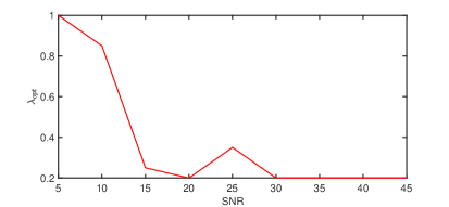
Figure 3: The value of optimal $\lambda$ versus varying SNR for CS_sparse. Here, we set $M=25,N=60,L=80,K=4,J=2000$, and $\kappa=20$.

We then compare the performance of each CS system with varying SNR level in (22). The results are displayed in Figure 5. This experiment indicates CS_MT, CS_MT-ETF, CS_sparse and CS_sparse-ETF outperform the others when SNR $<25$dB. We also see CS_MT-ETF and CS_sparse-ETF outperforms CS_MT and CS_sparse when SNR is high, respectively. Despite the high performance of CS_LYZCB when SNR $>25$dB, it decays fast as SNR decreases, which reveals CS_LYZCB is not robust to SRE. Interestingly, the corresponding sparse sensing matrices CS_sparse and CS_sparse-ETF have comparable performance as CS_MT and CS_MT-ETF, and are much better than CS_randn and CS_bispar.

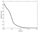
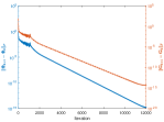
Figure 4: Convergence of Algorithm 1 in terms of (a) objective value, (b) the change of iterates $\{\bm{\Phi}\}_{k}$ (blue line) and $\{\bm{G}\}_{k}$ (red line). Here, we set $M=25,N=60,L=80,\lambda=0.25$ and $\kappa=20$.

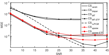
Figure 5: MSE versus different SNR (dB) for the signals in (22). Here, we set $M=25,N=60,L=80,K=4,J=2000,\lambda=0.25$ and $\kappa=20$. Disappearance from this figure means MSE is less than $10^{-5}$.

Finally, we investigate the change of signal recovery accuracy with varying $M$ and $K$. In Figures 6 and 7, we show the recovery accuracy versus various $M$ and $K$. We observe that our approach almost works the same as the dense one, CS_MT and CS_MT-ETF.

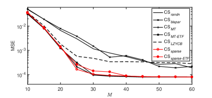
Figure 6: MSE versus different $M$ with SNR$=20$dB. Here, we set $N=60,L=80,K=4,J=2000,\lambda=0.25$ and $\kappa=20$.

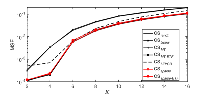
Figure 7: MSE versus different $K$ with SNR$=20$dB. Here, we set $M=25,N=60,L=80,J=2000,\lambda=0.25$ and $\kappa=20$.

5.2 Real Images

We now apply these CS systems to real image reconstruction from their sensing measurements. We examine the performance of the CS systems with two different sizes of dictionaries, a low dimensional dictionary $\bm{\Psi}\in\Re^{64\times 100}$ and a high dimensional one $\bm{\Psi}\in\Re^{256\times 800}$.

The low dimensional dictionary $\bm{\Psi}$ is learnt through KSVD algorithm [5] with a set of $\sqrt{N}\times\sqrt{N}$ non-overlapping patches by extracting randomly 15 patches from each of 400 images in the LabelMe [47] training data set. With each patch of $\sqrt{N}\times\sqrt{N}$ re-arranged as a vector of $N\times 1$, a set of $N\times 6000$ signals are obtained. Similarly, for learning a high dimensional dictionary, we extract more patches from the training dataset and obtains nearly $10^{6}$ signals since a high dimensional dictionary has much more parameters that need to be trained than a low dimensional dictionary. To address such a large training dataset, we choose the online dictionary learning algorithm [48] to learn this dictionary.

The performance of each CS system for real images is evaluated through Peak Signal to Noise Ratio (PSNR),

$$\text{PSNR}\triangleq 10\times\log{10\left[\frac{(2^{r}-1)^{2}}{\text{MSE}}\right]}\text{(dB)}$$

where $r=8$ bits per pixel and MSE is defined in (23).

We choose several test images to demonstrate the reconstruction performance in terms of PSNR. Since patch-based processing of images will introduce the artifact on boundary called blockiness, the deblocking techniques can be introduced here to act as a post-processing step to reduce such an artifact. To this end, we utilize the BM3D denoising algorithm as post-processing to tackle the blockiness [49]. We observe that such a post-processing step not only improves the visual effect, but also increases the PSNR for each method. To illustrate the improvement of the PSNR, we list the amount of increased PSNR by the post-processing in Tables 1 and 2 and Figure 10.

Table 1: Statistics of PSNR (dB) for six images with $M=20,\leavevmode\nobreak\ N=64,\leavevmode\nobreak\ L=100,\leavevmode\nobreak\ K=4,\leavevmode\nobreak\ \lambda=1.4$ using different $\kappa$. The performance of each CS system is described in two rows: the first row is the PSNR without post processing, while the second row is the amount of improved PSNR by post processing.

	Lena		Couple		Barbara		Child		Plane		Man
	$\kappa=10$	$\kappa=20$	$\kappa=10$	$\kappa=20$	$\kappa=10$	$\kappa=20$	$\kappa=10$	$\kappa=20$	$\kappa=10$	$\kappa=20$	$\kappa=10$	$\kappa=20$
CSrandn	$29.69$		$27.01$		$22.44$		$31.20$		$28.57$		$27.41$
	$+1.12$		$+0.95$		$+0.52$		$+1.27$		$+1.08$		$+1.04$
CSMT	$32.75$		$30.01$		$25.36$		$34.22$		$31.60$		$30.39$
	$+1.31$		$+1.05$		$+0.45$		$+1.72$		$+0.78$		$+0.32$
CSLZYCB	$12.74$		$10.38$		$\leavevmode\nobreak\ 4.19$		$15.93$		$14.51$		$\leavevmode\nobreak\ 9.75$
	$+1.58$		$+2.08$		$+7.32$		$+1.76$		$+1.33$		$+3.20$
CSbispar	$29.36$	$29.27$	$26.85$	$26.87$	$22.42$	$22.49$	$30.80$	$30.87$	$28.13$	$28.28$	$27.19$	$27.14$
	$+1.23$	$+1.24$	$+0.97$	$+1.03$	$+0.65$	$+0.61$	$+1.56$	$+1.46$	$+0.78$	$+0.90$	$+1.07$	$+1.09$
CSsparse-A	$32.38$	$32.65$	$29.63$	$29.88$	$24.91$	$25.19$	$33.84$	$34.12$	$31.28$	$31.52$	$30.01$	$30.27$
	$+1.86$	$+1.34$	$+1.31$	$+1.07$	$+1.04$	$+0.47$	$+2.03$	$+1.70$	$+0.85$	$+1.64$	$+0.44$	$+0.38$
CSsparse	$32.26$	$32.56$	$29.47$	$29.79$	$24.76$	$25.11$	$33.75$	$34.07$	$31.15$	$31.48$	$29.83$	$30.15$
	$+1.26$	$+1.33$	$+1.01$	$+1.02$	$+0.54$	$+0.47$	$+1.71$	$+1.68$	$+0.86$	$+1.21$	$+0.61$	$+0.40$

Table 2: Similar to Table 1, but with $M=80,\leavevmode\nobreak\ N=256,\leavevmode\nobreak\ L=800,\leavevmode\nobreak\ K=16,\leavevmode\nobreak\ \lambda=0.5$.

	Lena		Couple		Barbara		Child		Plane		Man
	$\kappa=10$	$\kappa=30$	$\kappa=10$	$\kappa=30$	$\kappa=10$	$\kappa=30$	$\kappa=10$	$\kappa=30$	$\kappa=10$	$\kappa=30$	$\kappa=10$	$\kappa=30$
CSrandn	$30.73$		$27.40$		$22.76$		$31.99$		$29.57$		$27.94$
	$+0.69$		$+0.51$		$+0.21$		$+0.59$		$+0.48$		$+0.48$
CSMT	$34.38$		$30.90$		$26.04$		$35.60$		$33.34$		$31.50$
	$+0.14$		$+0.23$		$+0.13$		$+0$		$+0.24$		$+0.20$
CSbispar	$30.23$	$30.72$	$27.33$	$27.36$	$22.57$	$22.64$	$31.70$	$31.94$	$29.29$	$29.49$	$27.59$	$27.82$
	$+0.67$	$+0.67$	$+0.50$	$+0.52$	$+0.21$	$+0.20$	$+0.58$	$+0.59$	$+0.48$	$+0.48$	$+0.46$	$+0.47$
CSsparse-A	$33.89$	$34.24$	$30.47$	$30.75$	$25.44$	$25.82$	$35.09$	$35.36$	$32.92$	$33.15$	$30.95$	$31.22$
	$+0.34$	$+0.22$	$+0.37$	$+0.29$	$+0.18$	$+0.16$	$+0.25$	$+0.08$	$+0.38$	$+0.29$	$+0.35$	$+0.27$
CSsparse	$33.17$	$33.50$	$29.69$	$29.94$	$24.26$	$24.60$	$34.38$	$34.66$	$32.41$	$32.61$	$30.06$	$30.39$
	$+0.45$	$+0.43$	$+0.42$	$+0.40$	$+0.15$	$+0.16$	$+0.24$	$+0.21$	$+0.38$	$+0.38$	$+0.35$	$+0.36$

With image Lena, we show the PSNR versus the sparsity $\kappa$ (the number of non-zero elements in each row of the sparse sensing matrix) in Figure 8. And furthermore, we list the performance statistics on other images including Couple, Barbara, Child, Plane, and Man in Tables 1 and 2. Figure 10 displays the visual result of “couple”.

As expected, CS_sparse-A and CS_sparse yield higher PSNR when increases the sparsity $\kappa$. It is interesting to see that although the sparsity is very low, for example, $\kappa=10$, CS_sparse-A is only 0.53dB inferior to CS_MT and still has more than $3$dB better than CS_randn which is a dense sensing matrix. We note that the gap between CS_sparse-A and CS_MT is almost negligible (with 0.15 dB) when $\kappa\geq 30$. This meets our argument that we can design a sparse sensing matrix instead of a dense matrix resulting in similar performance so that we can reduce the computational cost for sensing signals.

Figure 8 and Tables 1 and 2 indicate CS_sparse-A has better performance than CS_sparse because of $\bm{A}$ when $\kappa$ is small. This demonstrates the effect of utilizing the auxiliary DCT matrix for designing a structured sparse sensing matrix to increase the reconstruction accuracy.

It is not surprising to note that CS_LZYCB yields very low PSNR for real image experiments. This coincides with Figure 5 and further demonstrates that the sensing matrix in CS_LZYCB is not robust to the SRE. But we observe that the proposed sparse sensing matrices are robust to the SRE and hence the CS_sparse and CS_sparse-A have higher PSNR.

Comparing the results in Table 1 and Table 2, we observe that with a high dimensional dictionary, higher PSNR can be obtained. It is of great interest to note that the proposed sparse sensing matrix becomes extremely efficient for high dimensional patches since it can significantly reduce the sensing costs.

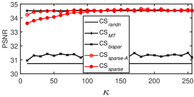
Figure 8: PSNR(dB) versus sparsity $\kappa$ for different CS systems without post-processing on image Lena. Here, $M=80,N=256,L=800,K=16,\lambda=0.5$.

Figure 9: The Original test image: “Couple”.

(a) CS_randn: $27.40$

(b) CS_bispar: $27.33$

(c) CS_sparse: $29.69$

(d) CS_sparse-A: $30.47$

(e) CS_MT: $30.90$

(f) $+0.51$

(g) $+0.50$

(h) $+0.42$

(i) $+0.37$

(j) $+0.23$

Figure 10: The PSNR (dB) of reconstructed images for different CS systems with $M=80,\leavevmode\nobreak\ N=256,\leavevmode\nobreak\ L=800,\leavevmode\nobreak\ K=16,\leavevmode\nobreak\ \lambda=0.5,\kappa=10$. Up: the PSNR without deblocking. Bottom: the amount of improved PSNR with deblocking.

6 Conclusions

We proposed a framework for designing a structured sparse sensing matrix that is robust to sparse representation error that widely exists for practical signals and can be efficiently implemented to sense signals. An alternating minimization-based algorithm is used to solve the optimal design problem, whose convergence is rigorously analyzed. The simulations demonstrate the promising performance of the proposed structured sparse sensing matrix in terms of signal reconstruction accuracy for synthetic data and real images.

As shown in Section 5, utilizing the base matrix $\bm{A}$ can improve the performance of the obtained sparse sensing matrix, especially when the number of non-zeros in $\bm{\Phi}$ is very small. Thus, it is of interest to utilize a base matrix $\bm{A}$ which has a few degrees of freedom (or parameters) that can be optimized, making it possible to simultaneously optimize the base matrix $\bm{A}$ and the sparse matrix $\bm{\Phi}$. One choice of such an idea is to utilize a series of Givens rotation matrices, which have parameters for choosing and can be implemented very efficiently, to act as the base matrix. We refer this to future work. It is also of interest to adopt the optimized structured sparse sensing matrix into analog-to-digital conversion system based on compressive sensing [50, 51]. Towards that end, it is important to develop a quantized (even 1-bit) sparse sensing matrix. We finally note that it remains an open problem to certify certain properties (such as the RIP) for the optimized sensing matrices [9, 10, 11, 12, 13, 14, 15, 16, 17, 18, 19], which empirically outperforms a random one that satisfies the RIP. Works in these directions are ongoing.

Appendix A Proof of 1

Proof.

We parametrize the function value through the line passing $[\bm{\Phi}^{\prime},\bm{\Phi}]$ by $t$, i.e., define $\upsilon(t)=f(\bm{\Phi}^{\prime}+t(\bm{\Phi}-\bm{\Phi}^{\prime}),\bm{G})$. It is clear that $\upsilon(0)=f(\bm{\Phi}^{\prime},\bm{G}),\leavevmode\nobreak\ \upsilon(1)=f(\bm{\Phi},\bm{G})$. Then we have

$$\upsilon(1)-\upsilon(0)=f(\bm{\Phi},\bm{G})-f(\bm{\Phi}^{\prime},\bm{G})=\int_{0}^{1}\upsilon^{\prime}(t)dt$$

$$=\int_{0}^{1}\langle\nabla_{\bm{\Phi}}f(\bm{\Phi}^{\prime}+t(\bm{\Phi}-\bm{\Phi}^{\prime}),\bm{G}),\bm{\Phi}-\bm{\Phi}^{\prime}\rangle dt$$

$$=\int_{0}^{1}\langle\nabla_{\bm{\Phi}}f(\bm{\Phi}^{\prime}+t(\bm{\Phi}-\bm{\Phi}^{\prime}),\bm{G})-\nabla_{\bm{\Phi}}f(\bm{\Phi}^{\prime},\bm{G}),\bm{\Phi}-\bm{\Phi}^{\prime}\rangle dt$$

$$\quad+\langle\nabla_{\bm{\Phi}}f(\bm{\Phi}^{\prime},\bm{G}),\bm{\Phi}-\bm{\Phi}^{\prime}\rangle$$

$$\leq\int_{0}^{1}\|\nabla_{\bm{\Phi}}f(\bm{\Phi}^{\prime}+t(\bm{\Phi}-\bm{\Phi}^{\prime}),\bm{G})-\nabla_{\bm{\Phi}}f(\bm{\Phi}^{\prime},\bm{G})\|_{F}dt$$

$$\quad\cdot\|\bm{\Phi}-\bm{\Phi}^{\prime}\|_{F}+\langle\nabla_{\bm{\Phi}}f(\bm{\Phi}^{\prime},\bm{G}),\bm{\Phi}-\bm{\Phi}^{\prime}\rangle$$

$$\leq L\|\bm{\Phi}-\bm{\Phi}^{\prime}\|_{F}^{2}\int_{0}^{1}tdt+\langle\nabla_{\bm{\Phi}}f(\bm{\Phi}^{\prime},\bm{G}),\bm{\Phi}-\bm{\Phi}^{\prime}\rangle$$

$$=\frac{L}{2}\|\bm{\Phi}-\bm{\Phi}^{\prime}\|_{F}^{2}+\langle\nabla_{\bm{\Phi}}f(\bm{\Phi}^{\prime},\bm{G}),\bm{\Phi}-\bm{\Phi}^{\prime}\rangle,$$

where in the last inequality we have used (17). ∎

Appendix B Proof of 1

We first state the following definition of subdifferential for a general lower semicontinuous function, which is not necessarily differentiable.

Definition 1.

(Subdifferentials [42]) Let $\sigma:\mathbb{R}^{d}\rightarrow(-\infty,\infty]$ be a proper and lower semicontinuous function, whose domain is defined as

$$\operatorname{dom}\sigma:=\left\{\bm{u}\in\mathbb{R}^{d}:\sigma(\bm{u})<\infty\right\}.$$

The Fréchet subdifferential $\partial_{F}\sigma$ of $\sigma$ at $\bm{u}$ is defined by

$$\partial_{F}\sigma(\bm{u})=\left\{\bm{z}:\lim_{\bm{v}\rightarrow\bm{u}}\inf\frac{\sigma(\bm{v})-\sigma(\bm{u})-\langle\bm{z},\bm{v}-\bm{u}\rangle}{\|\bm{u}-\bm{v}\|}\geq 0\right\}$$

for any $\bm{u}\in\operatorname{dom}\sigma$ and $\partial_{F}\sigma(\bm{u})=\emptyset$ if $\bm{u}\notin\operatorname{dom}\sigma$.

The subdifferential $\partial\sigma(\bm{u})$ of $\sigma$ at $\bm{u}\in\operatorname{dom}\sigma$ is defined as follows

$$\partial\sigma=\left\{\bm{z}:\exists\bm{u}_{k}\rightarrow\bm{u},\sigma(\bm{u}_{k})\rightarrow\sigma(\bm{u}),\bm{z}_{k}\in\partial_{F}\sigma(\bm{u}_{k})\rightarrow\bm{z}\right\}$$

We say $\bm{u}$ a critical point (a.k.a. stationary point) if subdifferential at $\bm{u}$ is $\bm{0}$. The set of critical points of $\sigma$ is denoted by $\mathcal{C}(\sigma)$.

Proof of Theorem 1.

We prove Theorem 1 by individually proving the four arguments.

Show (P1): It is clear that for any $k\in\mathbb{N}$, $\bm{\Phi}_{k}\in\mathcal{S}_{\kappa}$ and $\bm{G}_{k}\in\mathcal{G}_{\xi}$. Thus we have $\rho(\bm{\Phi}_{k},\bm{G}_{\ell})=f(\bm{\Phi}_{k},\bm{G}_{\ell})$ for any $k,\ell\in\mathbb{N}$. Let $\bm{B}=\bm{\Psi}^{\mathrm{T}}\bm{\Phi}_{k+1}^{\mathrm{T}}\bm{\Phi}_{k+1}\bm{\Psi}$. Noting that $\mathcal{G}_{\xi}$ is a closed convex set, we have

$$\left\langle\bm{G}-\mathcal{P}_{\mathcal{G}_{\xi}}(\bm{B}),\mathcal{P}_{\mathcal{G}_{\xi}}(\bm{B})-\bm{B}\right\rangle\geq 0,\ \forall\bm{G}\in\mathcal{G}_{\xi},$$

which directly implies

$$\rho(\bm{\Phi}_{k+1},\bm{G}_{k})-\rho(\bm{\Phi}_{k+1},\bm{G}_{k+1})$$

$$=\|\bm{G}_{k}-\bm{B}\|^{2}_{F}-\|\bm{G}_{k+1}-\bm{B}\|^{2}_{F}$$

$$=\|\bm{G}_{k}-\mathcal{P}_{\mathcal{G}_{\xi}}(\bm{B})+\mathcal{P}_{\mathcal{G}_{\xi}}(\bm{B})-\bm{B}\|^{2}_{F}-\|\mathcal{P}_{\mathcal{G}_{\xi}}(\bm{B})-\bm{B}\|^{2}_{F}$$

$$=\|\bm{G}_{k}-\mathcal{P}_{\mathcal{G}_{\xi}}(\bm{B})\|_{F}^{2}+2\left\langle\bm{G}_{k}-\mathcal{P}_{\mathcal{G}_{\xi}}(\bm{B}),\mathcal{P}_{\mathcal{G}_{\xi}}(\bm{B})-\bm{B}\right\rangle$$

$$\geq\|\bm{G}_{k}-\bm{G}_{k+1}\|_{F}^{2}\geq 0.$$

On the other hand, we rewrite (15) as

$$\begin{split}\bm{\Phi}_{k+1}&\in\mathcal{P}_{\mathcal{S}_{\kappa}}(\bm{\Phi}_{k}-\eta\nabla f(\bm{\Phi}_{k},\bm{G}_{k}))\\ &=\mathop{\rm argmin}_{\bm{Z}\in\mathcal{S}_{\kappa}}\|\bm{Z}-\left(\bm{\Phi}_{k}-\eta\nabla f(\bm{\Phi}_{k},\bm{G}_{k})\right)\|_{F}^{2}\\ &\in\mathop{\rm argmin}_{\bm{Z}\in\mathcal{S}_{\kappa}}h_{1/\eta}(\bm{Z},\bm{\Phi}_{k},\bm{G}_{k})\end{split}$$ (24)

which implies that

$$h_{1/\eta}(\bm{\Phi}_{k+1},\bm{\Phi}_{k},\bm{G}_{k}) \leq h_{1/\eta}(\bm{\Phi}_{k},\bm{\Phi}_{k},\bm{G}_{k})$$

$$=f(\bm{\Phi}_{k},\bm{G}_{k}).$$

This along with Lemma 1 gives

$$f(\bm{\Phi}_{k},\bm{G}_{k})-f(\bm{\Phi}_{k+1},\bm{G}_{k})$$

$$\geq f(\bm{\Phi}_{k},\bm{G}_{k})-h_{L_{c}}(\bm{\Phi}_{{k+1}},\bm{\Phi}_{k},\bm{G}_{k})$$

$$\geq h_{1/\eta}(\bm{\Phi}_{k+1},\bm{\Phi}_{k},\bm{G}_{k})-h_{L_{c}}(\bm{\Phi}_{{k+1}},\bm{\Phi}_{k},\bm{G}_{k})$$

$$=\frac{\frac{1}{\eta}-L_{c}}{2}\|\bm{\Phi}_{k}-\bm{\Phi}_{k+1}\|_{F}^{2}.$$

Show (P2): It follows from (18) that

$$\rho_{0}\geq\rho(\bm{\Phi}_{1},\bm{G}_{0})\geq\rho(\bm{\Phi}_{1},\bm{G}_{1})\geq\cdots\rho(\bm{\Phi}_{k},\bm{G}_{k})$$

$$\geq\rho(\bm{\Phi}_{k+1},\bm{G}_{k})\geq\rho(\bm{\Phi}_{k+1},\bm{G}_{k+1})\geq\cdots$$

which together with the fact that $\rho(\bm{\Phi}_{k},\bm{\Psi}_{k})\geq 0$ gives the convergence of sequence $\{\rho(\bm{\Phi}_{k},\bm{G}_{k})\}_{k\geq 0}$. This also implies that $(\bm{\Phi}_{k},\bm{G}_{k})\in\mathcal{L}_{\rho_{0}}$ and hence $\{(\bm{\Phi}_{k},\bm{G}_{k})\}_{k\geq 0}$ is a bounded sequence.

Show (P3): Utilizing (18) for all $k\in\mathbb{N}$ and summing them together, we obtain

$$\sum_{k=0}^{\infty}\frac{\frac{1}{\eta}-L_{c}}{2}\left(\|\bm{\Phi}^{k}-\bm{\Phi}^{k+1}\|_{F}^{2}\right)+\|\bm{G}^{k}-\bm{G}^{k+1}\|_{F}^{2}$$

$$\leq\rho_{0}-\lim_{k\rightarrow\infty}\rho(\bm{\Phi}_{k},\bm{G}_{k})\leq\rho_{0},$$

which implies that the series $\{\sum_{k=0}^{n}\|\bm{\Phi}^{k}-\bm{\Phi}^{k+1}\|_{F}^{2}+\|\bm{G}^{k}-\bm{G}^{k+1}\|_{F}^{2}\}_{n}$ is convergent. This together with the fact that $\|\bm{\Phi}^{k}-\bm{\Phi}^{k+1}\|_{F}^{2}\geq 0$ and $\|\bm{G}^{k}-\bm{G}^{k+1}\|_{F}^{2}\geq 0$ gives (19).

Show (P4): We rewrite (24) as

$$\bm{\Phi}_{k+1}\in\mathop{\rm argmin}_{\bm{\Phi}\in\mathbb{R}^{M\times N}}h_{\frac{1}{\eta}}(\bm{\Phi},\bm{\Phi}_{k},\bm{G}_{k})+\delta_{\mathcal{S}_{\kappa}}(\bm{\Phi}),$$ (25)

which implies (by the optimality of $\bm{\Phi}_{k+1}$ in (25) and letting $\bm{\Phi}=\underline{\bm{\Phi}}$, i.e. the limit of a convergent subsequence $\{\bm{\Phi}_{k^{\prime}}\}_{k^{\prime}}$)

$$\langle\nabla_{\bm{\Phi}}f(\bm{\Phi}_{k},\bm{G}_{k}),\bm{\Phi}_{k+1}-\bm{\Phi}_{k}\rangle+\frac{\eta}{2}\|\bm{\Phi}_{k+1}-\bm{\Phi}_{k}\|_{F}^{2}+\delta_{\mathcal{S}_{\kappa}}(\bm{\Phi}_{k+1})$$

$$\leq\langle\nabla_{\bm{\Phi}}f(\bm{\Phi}_{k},\bm{G}_{k}),\underline{\bm{\Phi}}-\bm{\Phi}_{k}\rangle+\frac{\eta}{2}\|\underline{\bm{\Phi}}-\bm{\Phi}_{k}\|_{F}^{2}+\delta_{\mathcal{S}_{\kappa}}(\underline{\bm{\Phi}}).$$

This further gives (take limit on subsequence $\{\bm{\Phi}_{k^{\prime}}\}_{k^{\prime}}$)

$$\begin{split}&\limsup_{k^{\prime}\rightarrow\infty}\delta_{\mathcal{S}_{\kappa}}(\bm{\Phi}_{k^{\prime}})-\delta_{\mathcal{S}_{\kappa}}(\underline{\bm{\Phi}})\\ &\leq\limsup_{k^{\prime}\rightarrow\infty}\langle\nabla_{\bm{\Phi}}f(\bm{\Phi}_{k^{\prime}-1},\bm{G}_{k^{\prime}-1}),\underline{\bm{\Phi}}-\bm{\Phi}_{k^{\prime}}\rangle\\ &\quad+\frac{\eta}{2}\|\bm{\Phi}_{k^{\prime}-1}-\underline{\bm{\Phi}}\|_{F}^{2}-\frac{\eta}{2}\|\bm{\Phi}_{k^{\prime}}-\bm{\Phi}_{k^{\prime}-1}\|_{F}^{2}\\ &=0,\end{split}$$ (26)

where the last line follows from (19), the fact that scalar product is continuous and $\lim_{k^{\prime}\rightarrow\infty}\|\bm{\Phi}_{k^{\prime}-1}-\underline{\bm{\Phi}}\|_{F}=0$ since

$$0 \leq\lim_{k^{\prime}\rightarrow\infty}\|\bm{\Phi}_{k^{\prime}-1}-\underline{\bm{\Phi}}\|_{F}$$

$$=\lim_{k^{\prime}\rightarrow\infty}\|\bm{\Phi}_{k^{\prime}-1}-\bm{\Phi}_{k^{\prime}}+\bm{\Phi}_{k^{\prime}}-\underline{\bm{\Phi}}\|_{F}$$

$$\leq\lim_{k^{\prime}\rightarrow\infty}\|\bm{\Phi}_{k^{\prime}}-\underline{\bm{\Phi}}\|_{F}+\|\bm{\Phi}_{k^{\prime}}-\bm{\Phi}_{k^{\prime}-1}\|_{F}=0.$$

From the fact that $\delta_{\mathcal{S}_{\kappa}}(\bm{\Phi})$ is lower semi-continuous, we have

$$\delta_{\mathcal{S}_{\kappa}}(\underline{\bm{\Phi}})\leq\liminf_{k^{\prime}\rightarrow\infty}\delta_{\mathcal{S}_{\kappa}}(\bm{\Phi}_{k^{\prime}}).$$

Utilizing (26) gives

$$\limsup_{k^{\prime}\rightarrow\infty}\delta_{\mathcal{S}_{\kappa}}(\bm{\Phi}_{k^{\prime}})\leq\delta_{\mathcal{S}_{\kappa}}(\underline{\bm{\Phi}})\leq\liminf_{k^{\prime}\rightarrow\infty}\delta_{\mathcal{S}_{\kappa}}(\bm{\Phi}_{k^{\prime}}),$$

which together with the fact

$$\liminf_{k^{\prime}\rightarrow\infty}\delta_{\mathcal{S}_{\kappa}}(\bm{\Phi}_{k^{\prime}})\leq\limsup_{k^{\prime}\rightarrow\infty}\delta_{\mathcal{S}_{\kappa}}(\bm{\Phi}_{k^{\prime}})$$

gives

$$\delta_{\mathcal{S}_{\kappa}}(\underline{\bm{\Phi}})=\liminf_{k^{\prime}\rightarrow\infty}\delta_{\mathcal{S}_{\kappa}}(\bm{\Phi}_{k^{\prime}})=\limsup_{k^{\prime}\rightarrow\infty}\delta_{\mathcal{S}_{\kappa}}(\bm{\Phi}_{k^{\prime}}),$$

and hence

$$\lim_{k^{\prime}\rightarrow\infty}\delta_{\mathcal{S}_{\kappa}}(\bm{\Phi}_{k^{\prime}})=\delta_{\mathcal{S}_{\kappa}}(\underline{\bm{\Phi}}).$$

Since $\mathcal{G}_{\xi}$ is a compact set and $\bm{G}_{k^{\prime}}\in\mathcal{G}_{\xi},\ \forall\ k^{\prime}\in\mathbb{N}$, we have the limit point $\underline{\bm{G}}\in\mathcal{G}_{\xi}$. Therefore, we obtain

$$\lim_{k^{\prime}\rightarrow\infty}\rho(\bm{\Phi}_{k^{\prime}},\bm{G}_{k^{\prime}}) =\lim_{k^{\prime}\rightarrow\infty}f(\bm{\Phi}_{k^{\prime}},\bm{G}_{k^{\prime}})+\delta_{\mathcal{S}_{\kappa}}(\bm{\Phi}_{k^{\prime}})+\delta_{\mathcal{G}_{\xi}}(\bm{G}_{k^{\prime}})$$

$$=\rho(\underline{\bm{\Phi}},\underline{\bm{G}}).$$

The remaining part is to prove that $\underline{\bm{W}}=(\underline{\bm{\Phi}},\underline{\bm{G}})$ is a stationary point of $\rho$, which is equivalent to show $(\bm{0},\bm{0})\in\partial\rho(\underline{\bm{\Phi}},\underline{\bm{G}})$. In what follows, we show a stronger result that $({\bf 0},{\bf 0})\in\lim_{k\rightarrow\infty}\partial\rho(\bm{\Phi}_{k},\bm{G}_{k})$.

First note that

$$\bm{G}_{k} =\mathop{\rm argmin}_{\bm{G}\in\mathbb{R}^{L\times L}}\rho(\bm{\Phi}_{k},\bm{G})$$

The optimality condition gives [44]

$${\bf 0}=\underbrace{\nabla_{\bm{G}}f(\bm{\Phi}_{k},\bm{G}_{k})+\bm{U}_{k}}_{\bm{D}_{\bm{G}_{k}}}\in\partial_{\bm{G}}\rho(\bm{W}_{k}),$$ (27)

where $\bm{U}_{k}\in\partial\delta_{\mathcal{G}_{\xi}}(\bm{G}_{k})$. On the other hand, the optimality condition of (25) gives (by setting $k\leftarrow k-1$ in (25))

$$\nabla_{\bm{\Phi}}f(\bm{\Phi}_{k-1},\bm{G}_{k-1})+\frac{1}{\eta}(\bm{\Phi}_{k}-\bm{\Phi}_{k-1})+\bm{V}_{k}=\bm{0},$$

where $\bm{V}_{k}\in\partial\delta_{\mathcal{S}_{\kappa}}(\bm{\Phi}_{k})$. Thus we have

$$\underbrace{\nabla_{\bm{\Phi}}f(\bm{W}_{k})-\nabla_{\bm{\Phi}}f(\bm{W}_{k-1})-\frac{1}{\eta}(\bm{\Phi}_{k}-\bm{\Phi}_{k-1})}_{\bm{D}_{\bm{\Phi}_{k}}}\in\partial_{\bm{\Phi}}\rho(\bm{W}_{k}),$$

which along with (27) gives

$$\left\|(\bm{D}_{\bm{\Phi}_{k}},\bm{D}_{\bm{G}_{k}})\right\|_{F}=\left\|\bm{D}_{\bm{\Phi}_{k}}\right\|_{F}$$

$$=\|\nabla_{\bm{\Phi}}f(\bm{W}_{k})-\nabla_{\bm{\Phi}}f(\bm{W}_{k-1})-\frac{1}{\eta}(\bm{\Phi}_{k}-\bm{\Phi}_{k-1})\|_{F}$$

$$\leq\|\nabla_{\bm{\Phi}}f(\bm{W}_{k})-\nabla_{\bm{\Phi}}f(\bm{\Phi}_{k},\bm{G}_{k-1})\|$$

$$\quad+\|\nabla_{\bm{\Phi}}f(\bm{\Phi}_{k},\bm{G}_{k-1})-\nabla_{\bm{\Phi}}f(\bm{W}_{k-1})\|$$

$$\quad+\frac{1}{\eta}\|\bm{\Phi}_{k}-\bm{\Phi}_{k-1}\|_{F}$$

$$\leq L_{c}\|\bm{G}_{k}-\bm{G}_{k-1}\|_{F}+(L_{c}+\frac{1}{\eta})\|\bm{\Phi}_{k}-\bm{\Phi}_{k-1}\|_{F}$$

$$\leq(2L_{c}+\frac{1}{\eta})\|\bm{W}_{k}-\bm{W}_{k-1}\|_{F},$$ (28)

where we have used the Lipschitz gradient (17) in the second inequality.

Applying (19), we finally obtain

$$\lim_{k\rightarrow\infty}(\bm{D}_{\bm{\Phi}_{k}},\bm{D}_{\bm{G}_{k}})=({\bf 0},{\bf 0})$$

since

$$\lim_{k\rightarrow\infty}\left\|(\bm{D}_{\bm{\Phi}_{k}},\bm{D}_{\bm{G}_{k}})\right\|_{F}=0.$$

Thus $({\bf 0},{\bf 0})\in\lim_{k\rightarrow\infty}\partial\rho(\bm{\Phi}_{k},\bm{G}_{k})$ and we conclude that any convergent subsequence of $\{\bm{W}_{k}\}$ converges to a stationary point of (16).

Finally, the statement

$$\lim_{k\rightarrow\infty}\rho(\bm{W}_{k})=\rho(\underline{\bm{W}}).$$

directly follows from (P2) that the objective value sequence $\{\rho(\bm{W}_{k})\}_{k\in\mathbb{N}}$ is convergent.

∎

Appendix C Proof of 2

We first state the definition of Kurdyka-Lojasiewicz (KL) inequality, which is proved to be useful for convergence analysis [42, 43, 44].

Definition 2.

A proper semi-continuous function $\sigma(\bm{u})$ is said to satisfy Kurdyka-Lojasiewicz (KL) inequality, if $\underline{\bm{u}}$ is a stationary point of $\sigma(\bm{u})$, then $\exists\leavevmode\nobreak\ \delta>0,\leavevmode\nobreak\ \theta\in[0,1),\leavevmode\nobreak\ C_{1}>0,\leavevmode\nobreak\ s.t.$

$$\left|\sigma(\bm{u})-\sigma(\underline{\bm{u}})\right|^{\theta}\leq C_{1}\|\bm{v}\|,\leavevmode\nobreak\ \leavevmode\nobreak\ \forall\leavevmode\nobreak\ \bm{u}\in B(\underline{\bm{u}},\delta),\leavevmode\nobreak\ \forall\leavevmode\nobreak\ \bm{v}\in\partial\sigma(\bm{u})$$

It is clear that our objective function $\rho(\bm{\Phi},\bm{G})$ is lower semi-continuous and it satisfies the above KL inequality since the three components $f(\bm{\Phi},\bm{G})$, $\delta_{\mathcal{S}_{\kappa}}(\bm{\Phi})$ and $\delta_{\mathcal{G}_{\xi}}(\bm{G})$ all have the KL inequality [43, 44].

Proof of Theorem 2.

1 reveals the subsequential convergence property of the iterates sequence $\{\bm{W}_{k}=(\bm{\Phi}_{k},\bm{G}_{k})\}_{k}$, i.e., the limit point of any convergent subsequence converges to a stationary point. In what follows, we show the sequence $\{\bm{W}_{k}=(\bm{\Phi}_{k},\bm{G}_{k})\}_{k}$ itself is indeed convergent, and hence it converges to a certain stationary point of $\underline{\bm{W}}=(\underline{\bm{\Phi}},\underline{\bm{G}})$.

It follows from (20) that for any $\delta>0$, there exists an integer $n$ such that $\bm{W}_{k}\in B(\underline{\bm{W}},\delta),\leavevmode\nobreak\ \forall\leavevmode\nobreak\ k>n$ for some stationary point $\underline{\bm{W}}\in\mathcal{C}(\rho)$. From the concavity of the function $h(y)=y^{1-\theta}$ with domain $y>0$, we have

$$\left[\rho(\bm{W}_{k+1})-\rho(\underline{\bm{W}})\right]^{1-\theta}$$ (29)

$$\leq\left[\rho(\bm{W}_{k})-\rho(\underline{\bm{W}})\right]^{1-\theta}+(1-\theta)\frac{\rho(\bm{W}_{k+1})-\rho(\bm{W}_{k})}{\left[\rho(\bm{W}_{k})-\rho(\underline{\bm{W}})\right]^{\theta}}.$$

We now provide lower bound and upper bound for $\rho(\bm{W}_{k})-\rho(\bm{W}_{k+1})$ and $\left[\rho(\bm{W}_{k})-\rho(\underline{\bm{W}})\right]^{\theta}$, respectively. It follows from (18) that

$$\rho(\bm{W}_{k})-\rho(\bm{W}_{k+1})\geq C_{2}\|\bm{W}_{k+1}-\bm{W}_{k}\|_{F}^{2},$$

where $C_{2}=\min\{\frac{\frac{1}{\eta}-L_{c}}{2},1\}$. On the other hand, from (28) and the KL inequality we have

$$\left[\rho(\bm{W}_{k})-\rho(\underline{\bm{W}})\right]^{\theta} \leq C_{1}\left\|(\bm{D}_{\bm{\Phi}_{k}},\bm{D}_{\bm{G}_{k}})\right\|_{F}$$

$$\leq C_{3}\|\bm{W}_{k}-\bm{W}_{k-1}\|_{F},$$

where $C_{3}=C_{1}(2L_{c}+1/\eta)$. Plugging the above two inequalities into (29) gives

$$\left[\rho(\bm{W}_{k})-\rho(\underline{\bm{W}})\right]^{1-\theta}-\left[\rho(\bm{W}_{k+1})-\rho(\underline{\bm{W}})\right]^{1-\theta}$$

$$\geq(1-\theta)\frac{C_{2}\|\bm{W}_{k+1}-\bm{W}_{k}\|_{F}^{2}}{C_{3}\|\bm{W}_{k}-\bm{W}_{k-1}\|_{F}}.$$ (30)

Let $C_{4}=(1-\theta)C_{2}/C_{3}$. Repeating the above equation for $k$ from $1$ to $\infty$ and summing them gives

$$\frac{1}{C_{4}}\left[\rho(\bm{W}_{1})-\rho(\underline{\bm{W}})\right]^{1-\theta}-\frac{1}{C_{4}}\left[\rho(\bm{W}_{\infty})-\rho(\underline{\bm{W}})\right]^{1-\theta}$$

$$\geq\sum_{k=1}^{\infty}\frac{\|\bm{W}_{k+1}-\bm{W}_{k}\|_{F}^{2}}{\|\bm{W}_{k}-\bm{W}_{k-1}\|_{F}}+\|\bm{W}_{k}-\bm{W}_{k-1}\|_{F}$$

$$\quad-\|\bm{W}_{k}-\bm{W}_{k-1}\|_{F}$$

$$\stackrel{{\scriptstyle(i)}}{{\geq}}2\sum_{k=1}^{\infty}\|\bm{W}_{k+1}-\bm{W}_{k}\|_{F}-\sum_{k=1}^{\infty}\|\bm{W}_{k}-\bm{W}_{k-1}\|_{F}$$

$$=\sum_{k=1}^{\infty}\|\bm{W}_{k+1}-\bm{W}_{k}\|_{F}-\|\bm{W}_{1}-\bm{W}_{0}\|_{F},$$

where $(i)$ is from the arithmetic inequality, i.e., $a^{2}+b^{2}\geq 2ab$. The proof is completed by applying the above result with the boundedness of $\{\bm{W}_{k}\}_{k}$ and (20):

$$\sum_{k=1}^{\infty}\|\bm{W}_{k+1}-\bm{W}_{k}\|_{F}<\infty$$

which implies that the sequence $\{\bm{W}_{k}\}_{k\in\mathbb{N}}$ is Cauchy [44] in a compact set and hence it is convergent. ∎

Appendix D The Choice of Step Size With Unknown Lipschitz Constant $L_{c}$

In practice, it is challenge to choose an appropriate step size since it is not easy to compute the Lipschitz constant $L_{c}$. According to the given convergence analysis in Section 4, we know if the step size is chosen to satisfy (18), the convergence is still guaranteed. Thus, we can utilize the backtracking method [52] with inequality (18) to search an appropriate step size without knowing $L_{c}$. The procedure is detailed in Algorithm 2.

Algorithm 2 Backtracking Procedure

0:   Initial value: $(\eta_{0},\gamma,\alpha)$ where $\eta_{0}$ is the initial guess step size, $\gamma\in(0,1)$ and $\alpha\in(0,1)$.

0:   Step size $\eta$ and Updated $\bm{\Phi}_{k+1}$.

1:  $\eta\leftarrow\eta_{0}$

2:  $\bm{\Phi}_{k+1}\leftarrow\mathcal{P}_{\mathcal{S}_{\kappa}}(\bm{\Phi}_{k}-\eta\nabla_{\bm{\Phi}}f(\bm{\Phi}_{k},\bm{G}_{k}))$

3:  while $\rho(\bm{\Phi}_{k},\bm{G}_{k})-\rho(\bm{\Phi}_{k+1},\bm{G}_{k})<\frac{\gamma}{2\eta}\|\bm{\Phi}_{k+1}-\bm{\Phi}_{k}\|_{F}^{2}$ do

4:     $\eta\leftarrow\alpha\eta$

5:     Update $\bm{\Phi}_{k+1}$: $\bm{\Phi}_{k+1}\leftarrow\mathcal{P}_{\mathcal{S}_{\kappa}}(\bm{\Phi}_{k}-\eta\nabla_{\bm{\Phi}}f(\bm{\Phi}_{k},\bm{G}_{k}))$

6:  end while

References

- [1] E. Candès, J. Romberg, and T. Tao, “Robust uncertainty principles: Exact signal reconstruction from highly incomplete frequency information,” IEEE Trans. Inf. Theory, vol. 52, no. 2, pp. 489–509, 2006.
- [2] E. Candès and M. B. Wakin, “An introduction to compressive sampling,” IEEE Signal Process. Mag., vol. 25, no. 2, pp. 21–30, 2008.
- [3] Z. Zhu and M. B. Wakin, “Approximating sampled sinusoids and multiband signals using multiband modulated DPSS dictionaries,” to appear in J. Fourier Anal. Appl.
- [4] K. Engan, S. O. Aase, and J. Hakon Husoy, “Method of optimal directions for frame design,” in Proc. IEEE Int. Conf. Acoust., Speech, and Signal Processing (ICASSP), vol. 5, pp. 2443–2446, 1999.
- [5] M. Aharon, M. Elad, and A. Bruckstein, “K-SVD: An algorithm for designing overcomplete dictionaries for sparse representation,” IEEE Trans. Signal Process., vol. 54, no. 11, pp. 4311–4322, 2006.
- [6] G. Li, Z. Zhu, H. Bai, and A. Yu, “A new framework for designing incoherent sparsifying dictionaries,” in IEE Int. Conf. Acous. Speech, Signal Process. (ICASSP), pp. 4416–4420, IEEE, 2017.
- [7] R. Baraniuk, M. Davenport, R. DeVore, and M. Wakin, “A simple proof of the restricted isometry property for random matrices,” Constructive Approx., vol. 28, no. 3, pp. 253–263, 2008.
- [8] A. S. Bandeira, E. Dobriban, D. G. Mixon, and W. F. Sawin, “Certifying the restricted isometry property is hard,” IEEE Trans. Inf. Theory, vol. 59, no. 6, pp. 3448–3450, 2013.
- [9] M. Elad, “Optimized projections for compressed sensing,” IEEE Trans. Signal Process., vol. 55, no. 12, pp. 5695–5702, 2007.
- [10] J. M. Duarte-Carvajalino and G. Sapiro, “Learning to sense sparse signals: Simultaneous sensing matrix and sparsifying dictionary optimization,” IEEE Trans. Image Process., vol. 18, no. 7, pp. 1395–1408, 2009.
- [11] V. Abolghasemi, S. Ferdowsi, and S. Sanei, “A gradient-based alternating minimization approach for optimization of the measurement matrix in compressive sensing,” Signal Process., vol. 92, no. 4, pp. 999–1009, 2012.
- [12] G. Li, Z. Zhu, D. Yang, L. Chang, and H. Bai, “On projection matrix optimization for compressive sensing systems,” IEEE Trans. Signal Process., vol. 61, no. 11, pp. 2887–2898, 2013.
- [13] W. Chen, M. R. Rodrigues, and I. J. Wassell, “Projection design for statistical compressive sensing: A tight frame based approach,” IEEE Trans. Signal Process., vol. 61, no. 8, pp. 2016–2029, 2013.
- [14] G. Li, X. Li, S. Li, H. Bai, Q. Jiang, and X. He, “Designing robust sensing matrix for image compression,” IEEE Trans. Image Process., vol. 24, no. 12, pp. 5389–5400, 2015.
- [15] H. Bai, G. Li, S. Li, Q. Li, Q. Jiang, and L. Chang, “Alternating optimization of sensing matrix and sparsifying dictionary for compressed sensing,” IEEE Transactions on Signal Processing, vol. 63, no. 6, pp. 1581–1594.
- [16] T. Hong, H. Bai, S. Li, and Z. Zhu, “An efficient algorithm for designing projection matrix in compressive sensing based on alternating optimization,” Signal Process., vol. 125, pp. 9–20, 2016.
- [17] T. Hong and Z. Zhu, “An efficient method for robust projection matrix design,” Signal Process., vol. 143, no. 3, pp. 200–210, 2018.
- [18] X. Li, H. Bai, and B. Hou, “A gradient-based approach to optimization of compressed sensing systems,” Signal Processing, vol. 139, pp. 49–61, 2017.
- [19] Z. Zhu, G. Li, J. Ding, Q. Li, and X. He, “On collaborative compressive sensing systems: The framework, design, and algorithm,” SIAM J. Imaging Sci., vol. 11, no. 2, pp. 1717–1758, 2018.
- [20] W. Yin, S. Morgan, J. Yang, and Y. Zhang, “Practical compressive sensing with toeplitz and circulant matrices,” in Visual Communications and Image Processing 2010, vol. 7744, p. 77440K, International Society for Optics and Photonics, 2010.
- [21] G. Zhang, S. Jiao, X. Xu, and L. Wang, “Compressed sensing and reconstruction with bernoulli matrices,” in Information and Automation (ICIA), 2010 IEEE International Conference on, pp. 455–460, IEEE, 2010.
- [22] U. Dias and M. E. Rane, “Comparative analysis of sensing matrices for compressed sensed thermal images,” in Automation, Computing, Communication, Control and Compressed Sensing (iMac4s), 2013 International Multi-Conference on, pp. 265–270, IEEE, 2013.
- [23] J. Sun, S. Wang, and Y. Dong, “Sparse block circulant matrices for compressed sensing,” IET Communications, vol. 7, no. 13, pp. 1412–1418, 2013.
- [24] F. Fan, “Toeplitz-structured measurement matrix construction for chaotic compressive sensing,” in Intelligent Control and Information Processing (ICICIP), 2014 Fifth International Conference on, pp. 19–22, IEEE, 2014.
- [25] L. Gan, T. T. Do, and T. D. Tran, “Fast compressive imaging using scrambled block hadamard ensemble,” in Signal Processing Conference, 2008 16th European, pp. 1–5, IEEE, 2008.
- [26] H. Rauhut, “Compressive sensing and structured random matrices,” Theoretical foundations and numerical methods for sparse recovery, vol. 9, pp. 1–92, 2010.
- [27] F. Chen, A. P. Chandrakasan, and V. M. Stojanovic, “Design and analysis of a hardware-efficient compressed sensing architecture for data compression in wireless sensors,” IEEE J. Solid-State Circuits, vol. 47, no. 3, pp. 744–756, 2012.
- [28] Y. Dou, S. Vassiliadis, G. K. Kuzmanov, and G. N. Gaydadjiev, “64-bit floating-point fpga matrix multiplication,” in Proceedings of the 2005 ACM/SIGDA 13th international symposium on Field-programmable gate arrays, pp. 86–95, ACM, 2005.
- [29] H. Mamaghanian, N. Khaled, D. Atienza, and P. Vandergheynst, “Compressed sensing for real-time energy-efficient ecg compression on wireless body sensor nodes,” IEEE T. Biom. Engineer., vol. 58, no. 9, pp. 2456–2466, 2011.
- [30] A. Gilbert and P. Indyk, “Sparse recovery using sparse matrices,” Proceedings of the IEEE, vol. 98, no. 6, pp. 937–947, 2010.
- [31] T. Strohmer and R. W. Heath, “Grassmannian frames with applications to coding and communication,” Appl. Comput. Harmon. Anal., vol. 14, no. 3, pp. 257–275, 2003.
- [32] M. Elad, Sparse and Redundant Representations: From Theory to Applications in Signal and Image Processing. Springer Publishing Company, Incorporated, 1st ed., 2010.
- [33] S. S. Chen, D. L. Donoho, and M. A. Saunders, “Atomic decomposition by basis pursuit,” SIAM J. Sci. Comput., vol. 20, no. 1, pp. 33–61, 1998.
- [34] D. L. Donoho and M. Elad, “Optimally sparse representation in general (nonorthogonal) dictionaries via minimization,” Proc. Natt. Acad. Sci., vol. 100, no. 5, pp. 2197–2202, 2003.
- [35] J. A. Tropp, “Greed is good: Algorithmic results for sparse approximation,” IEEE Trans. Inf. Theory, vol. 50, no. 10, pp. 2231–2242, 2004.
- [36] W.-S. Lu and T. Hinamoto, “Design of projection matrix for compressive sensing by nonsmooth optimization,” in Circuits and Systems (ISCAS), 2014 IEEE International Symposium on, pp. 1279–1282, IEEE, 2014.
- [37] J. Sulam, B. Ophir, M. Zibulevsky, and M. Elad, “Trainlets: Dictionary learning in high dimensions,” IEEE Transactions on Signal Processing, vol. 64, no. 12, pp. 3180–3193, 2016.
- [38] R. Rubinstein, M. Zibulevsky, and M. Elad, “Double sparsity: Learning sparse dictionaries for sparse signal approximation,” IEEE Trans. Signal Process., vol. 58, no. 3, pp. 1553–1564, 2010.
- [39] P. Dita, “Factorization of unitary matrices,” Journal of Physics A: Mathematical and General, vol. 36, no. 11, p. 2781, 2003.
- [40] Z. Zhu, Q. Li, G. Tang, and M. B. Wakin, “Global optimality in low-rank matrix optimization,” IEEE Trans. Signal Process., vol. 66, no. 13, pp. 3614–3628, 2018.
- [41] Q. Li, Z. Zhu, and G. Tang, “The non-convex geometry of low-rank matrix optimization,” Information and Inference: A Journal of the IMA, p. iay003, 2018.
- [42] H. Attouch, J. Bolte, P. Redont, and A. Soubeyran, “Proximal alternating minimization and projection methods for nonconvex problems: An approach based on the kurdyka-lojasiewicz inequality,” Mathematics of Operations Research, vol. 35, no. 2, pp. 438–457, 2010.
- [43] H. Attouch, J. Bolte, and B. F. Svaiter, “Convergence of descent methods for semi-algebraic and tame problems: proximal algorithms, forward–backward splitting, and regularized gauss–seidel methods,” Math. Program., vol. 137, no. 1-2, pp. 91–129, 2013.
- [44] J. Bolte, S. Sabach, and M. Teboulle, “Proximal alternating linearized minimization for nonconvex and nonsmooth problems,” Math. Program., vol. 146, no. 1-2, pp. 459–494, 2014.
- [45] T. Blumensath and M. E. Davies, “Iterative hard thresholding for compressed sensing,” Applied and computational harmonic analysis, vol. 27, no. 3, pp. 265–274, 2009.
- [46] A. Beck and Y. C. Eldar, “Sparsity constrained nonlinear optimization: Optimality conditions and algorithms,” SIAM J. Optimiz., vol. 23, no. 3, pp. 1480–1509, 2013.
- [47] B. C. Russell, A. Torralba, K. P. Murphy, and W. T. Freeman, “Labelme: a database and web-based tool for image annotation,” Int. J. Computer Vision, vol. 77, no. 1, pp. 157–173, 2008.
- [48] J. Mairal, F. Bach, J. Ponce, and G. Sapiro, “Online dictionary learning for sparse coding,” in Proc. the 26th ann. int. conf. machine learning(ICML), pp. 689–696, ACM, 2009.
- [49] K. Dabov, A. Foi, V. Katkovnik, and K. Egiazarian, “Image denoising by sparse 3-d transform-domain collaborative filtering,” IEEE Transactions on image processing, vol. 16, no. 8, pp. 2080–2095, 2007.
- [50] J. A. Tropp, J. N. Laska, M. F. Duarte, J. K. Romberg, and R. G. Baraniuk, “Beyond nyquist: Efficient sampling of sparse bandlimited signals,” IEEE Trans. Inform. Theory, vol. 56, no. 1, pp. 520–544, 2010.
- [51] M. A. Davenport and M. B. Wakin, “Compressive sensing of analog signals using discrete prolate spheroidal sequences,” Applied and Computational Harmonic Analysis, vol. 33, no. 3, pp. 438–472, 2012.
- [52] J. Nocedal and S. Wright, Numerical Optimization. Springer Science & Business Media, 2006.