Evolution of Compact Stars and Dark Dynamical Variables

Abstract

This work is aimed to explore the dark dynamical effects of $f(R,T)$ modified gravity theory on the dynamics of compact celestial star. We have taken the interior geometry as spherical star which is filled with imperfect fluid distribution. The modified field equations are explored by taking a particular form of $f(R,T)$ model, i.e., $f(R,T)=f_{1}(R)+f_{2}(R)f_{3}(T)$. These equations are then utilized to formulate the well-known structure scalars under the dark dynamical effects of this higher order gravity theory. Also, the evolution equations for expansion and shear are formulated with the help of these scalar variables. Further, all this analysis have been made under the condition of constant $R$ and $T$. We found a crucial significance of dark source terms and dynamical variables on the evolution and density inhomogeneity of compact objects.

Keywords: Gravitation; Structure scalars; Relativistic dissipative fluids.
PACS: 04.40.-b, 04.40.Nr, 04.40.Dg

1 Introduction

After many observational astronomical consequences coming from Supernovae Type Ia, BICEP, and cosmic microwave background radiation [1, 2, 3], it has been affirmed that our cosmos is in accelerated expanding phase. Dark energy (DE) is thought to be reliable source behind this enigmatic behavior of the universe. In order to deal with its nature, the modified gravity theories are believed to be one of the mathematical tools. These theories are explored by modifying the Einstein-Hilbert (EH) action and extensively been applied to study the nature and problem of DE, that may lead to confront with accelerating cosmic expansion [4, 5, 6, 7].

Nojiri and Odintsov [8] introduced some modified gravitational models for the complete description of early and late-time evolutionary universe eras. The simplest generalization of GR includes $f(R)$ gravity in which $R$ is the Ricci scalar. Harko et al. [9] modified this theory by invoking corrections coming from the trace of energy-momentum tensor ($T$) in the EH action. This theory is widely known as $f(R,T)$ gravity theory. The motivation of this theory stems from the fact that the influences introduced by quantum effects or dark non-ideal relativistic matter environment are being invoked in this analysis.

Houndjo [10] obtained some observationally well-consistent $f(R,T)$ models that could assist enough to analyze the behavior of matter dominated universe epochs. Baffou et al. [11] used perturbation scheme to investigate the viability of few cosmic models by taking de-Sitter and power law formulations. Bamba et al. [12] checked the role of dark source terms coming from modified gravity models on the dynamics of accelerating and expanding universe. Durrer and Maartens [13] presented some results to the credibility of GR in terms of $f(R)$ gravity. Gravitational stabilities of relativistic compact structures were examined in in $f(R)$ gravity by [14, 15, 16]. Yousaf and his colleagues examined the rate of gravitational implosion with the help of various modified gravity models for the planar [17], spherical [18] as well as cylindrical [19] relativistic objects. Moraes et al. [20] calculated modified hydrostatic expression for investigating the dynamical features of some strange and neutron stars with the help of $f(R,T)=R+2\lambda T$ model.

Herrera et al. [21, 22] discussed the gravitational implosion of cylindrical as well as spherical collapse via some specific boundary conditions. Tewari et al. [23] investigated spherical anisotropic collapse and presented new class of relativistic models that could be helpful to understand various dynamical features of stellar models. Sharif and Bhatti [24] examined the role of adiabatic index as well as physical parameters on the onset of gravitational collapse of axially symmetric self-gravitating systems. Sharif and Yousaf [25, 26] considered the problem of dynamical instability of celestial bodies in modified gravity and found the role of $f(R,T)$ and $f(R)$ in the subsequent phases of collapsing systems. Recently, Yousaf et al. [27, 28] joined interior non-static anisotropic cylindrical system with exterior Einstein-Rosen bridge and investigated the impact of modified corrections on the onset of dynamical instability.

The inhomogeneous state is found to be the predecessor in the process of gravitational collapse for the initially homogenous stellar structures. It is pertinent to mention that one can understand some dynamical properties of self-gravitating systems through investigating the behavior of pressure anisotropy, tidal forces, inhomogeneous energy density (IED), etc. There has been extensive work related to check the cause of IED over the surface of regular compact objects. The work of Penrose and Hawking [29] is among pioneers works in this direction. They found Weyl tensor as a key figure in the emergence of IED in the evolution of spherically symmetric objects. Herrera et al. [30] calculated some factors responsible for creating IED over the anisotropic stellar spheres and inferred that pressure anisotropy may lead the system to develop naked singularity (NS). Virbhadra et al. [31, 32] provided a mathematical platform under which one can differentiate between the formation of NS and black holes.

Herrera et al. [33] described gravitational arrow of time for the dissipative compact systems by making a relation among Weyl invariant, pressure anisotropy and IED. Herrera et al. [34] examined the influences of IED on the expressions of shear and expansion evolutions in the presence of electromagnetic field. Yousaf et al. [35] covered this problem for spherical radiating geometries in modified gravitational theory and concluded that a special combination of $f(R,T)$ gravity model could significantly interfere in the appearance of IED. Bhatti and his colleagues [36] looked into the reasons behind the maintenance of IED against gravitational collapse of relativistic interiors in modified gravity. Herrera et al. [37] and Herrera [38] considered the case of non-comoving coordinate system and checked the reasons for the start up of the spherical collapse by evaluating transport equations. Yousaf et al. [39] modified these results by invoking Palatini $f(R)$ corrections. Recently, Herrera [40] illustrated the answer to the question that why observations of tilted congruences notice dissipative process in stellar interiors which seem to be isentropic for non-tilted observers.

This paper is a continuation of a previous work presented by Herrera et al. [34] in order to check the role of $f(R,T)=R+\lambda R^{2}T^{2}$ cosmic model in the formulations of structure scalars, shear and expansion evolution equations. The paper is outlined as under. Next section is devoted to describe some essential required to understand $f(R,T)$ gravity as well as spherical distribution of radiating fluids. In section 3, we shall compute modified form of structure scalars in the realm of $R+\lambda R^{2}T^{2}$ corrections. We shall also examine the role of shear and expansion evolution equations in this gravity. Section 4 demonstrates the role of scalar parameters in the emergence of IED of the dust relativistic cloud in today values of $R$ and $T$. The brief description as well as conclusion are reported in the last section.

2 Radiating Sphere and $f(R,T)$ Gravity

In $f(R,T)$ gravity, the EH action can be written as [9]

$$A=\int d^{4}x[f(R,T)+L_{M}]\sqrt{-g},$$ (1)

where $g,~{}T$ are the traces of metric and usual energy-momentum tensors, respectively, while $L_{M}$ is the matter Lagrangian. In the following calculations, we shall opt relativistic units that gives $8{\pi}G=c=1$. After considering $L_{M}=\mu$ (where $\mu$ is the fluid energy density) and applying variations in the above modified action with $g_{\alpha\beta}$, one can write field equations as

$${G}_{\lambda\nu}={{T}_{\lambda\nu}}^{\textrm{eff}},$$ (2)

where

$${{T}_{\lambda\nu}}^{\textrm{eff}} =\left[-\mu g_{\lambda\nu}f_{T}(R,T)+T^{(m)}_{\lambda\nu}(1+f_{T}(R,T))+\left(f_{R}(R,T)-\frac{f(R,T)}{R}\right)\frac{R}{2}\right.+$$

$$\left.+\left({\nabla}_{\lambda}{\nabla}_{\nu}+g_{\lambda\nu}{\Box}\right)f_{R}(R,T)\right]\frac{1}{f_{R}(R,T)}.$$

In Eq.(2), ${G}_{\alpha\beta}$ is the Einstein tensor, while ${{T}_{\lambda\nu}}^{\textrm{eff}}$ is widely known as effective form of energy-momentum tensor. However, $\nabla_{\alpha}$, $\Box$, $f_{T}(R,T)$ and $f_{R}(R,T)$ stand for covariant derivative, $\nabla_{\alpha}\nabla^{\alpha}$, partial derivatives with $R$ and $T$, respectively. One can visualize the detailed illustration of the field equations (2) from [9] and [35].

Let us consider an irrotational diagonal non-static form of spherically symmetric metric

$$ds^{2}=H^{2}(t,r)dr^{2}-A^{2}(t,r)dt^{2}+C^{2}(d\theta^{2}+\sin^{2}\theta{d\phi^{2}}),$$ (3)

in which $A,~{}B$ and $C$ depend on $t$ and $r$. It is assumed that above geometry is being coupled with radiating shear locally anisotropic fluid represented by

$$T_{\lambda\nu}={\mu}V_{\lambda}V_{\nu}+P_{\bot}h_{\lambda\nu}+\Pi\chi_{\lambda}\chi_{\nu}-2{\eta}{\sigma}_{\lambda\nu}+{\varepsilon}l_{\lambda}l_{\nu}+q(\chi_{\nu}V_{\lambda}+\chi_{\lambda}V_{\nu}),$$ (4)

where $\varepsilon$ is radiation density, $q_{\beta}$ is heat flux, $\Pi\equiv P_{r}-P_{\perp}$, $h_{\alpha\beta},~{}\sigma_{\alpha\beta}$ are projection and shear tensor, $P_{\bot},~{}P_{r}$ are tangential and radial pressure elements, $\mu$ is the energy density and $\eta$ is coefficient of shear viscosity. The projection tensor is defined as $h_{\alpha\beta}=g_{\alpha\beta}+V_{\alpha}V_{\beta}$, while $\chi^{\beta}$ and $l^{\beta}$ are radial and null four-vectors, respectively. Under co-moving coordinate system, the definitions of these vectors are found as $V^{\nu}=\frac{1}{A}\delta^{\nu}_{0},~{}\chi^{\nu}=\frac{1}{C}\delta^{\nu}_{1},~{}l^{\nu}=\frac{1}{A}\delta^{\nu}_{0}+\frac{1}{B}\delta^{\nu}_{1},~{}q^{\nu}=q(t,r)\chi^{\nu}$. In order to maintain comoving coordinate frame, these obey relations

$$\chi^{\nu}\chi_{\nu}=1,\quad V^{\nu}V_{\nu}=-1,\quad\chi^{\nu}V_{\nu}=0,$$

$$l^{\nu}V_{\nu}=-1,\quad V^{\nu}q_{\nu}=0,\quad l^{\nu}l_{\nu}=0.$$

With reference to Eq. (3), the shear tensor and scalar corresponding to expansion tensor are

$$\sigma A=\left(\frac{\dot{H}}{H}-\frac{\dot{C}}{C}\right),\quad\Theta A=\left(\frac{\dot{H}}{H}+\frac{2\dot{C}}{C}\right).$$

where overdot describes $\frac{\partial}{\partial t}$.

In order to have observationally well-consistent gravitational theory, one need to cope appropriate $f(R,T)$ gravity model. In this perspective, we take the following combinations of $f(R,T)$ model [41]

$$f(R,T)=f_{1}(R)+f_{2}(R)f_{3}(T).$$ (5)

This form of model description states a minimal background of matter and geometry coupling, thereby indicating higher order corrections in well-known a $f(R)$ theory. Realistic $f(R,T)$ models can be achieved by picking any Ricci scalar function from [42] along with any linear form of $T$ function. In this context, we shall take $f(R,T)=R+\lambda R^{2}T^{2}$, where $\lambda\ll 1$. The dynamics proposed by Einstein can be found on setting $\lambda=0$ in the above model. The $f(R,T)$ field equations for Eqs.(3)-(5) are

$$G_{00} =\frac{A^{2}}{1+2R\lambda T^{2}}\left[{\mu}+{\varepsilon}+2T\lambda R^{2}-\frac{\lambda}{2}T^{2}R^{2}+\frac{\varphi_{00}}{A^{2}}\right],$$ (6)

$$G_{01} =\frac{AH}{1+2R\lambda T^{2}}\left[-\frac{(1+2T\lambda R^{2})}{1+2R\lambda T^{2}}(q+{\varepsilon})+\frac{\varphi_{01}}{AH}\right],$$ (7)

$$G_{11} =\frac{H^{2}}{1+2R\lambda T^{2}}\left[\mu 2T\lambda R^{2}+(1+2T\lambda R^{2})(P_{r}+\varepsilon-\frac{4}{3}\eta{\sigma})+\frac{\lambda}{2}T^{2}R^{2}+\frac{\varphi_{11}}{H^{2}}\right],$$ (8)

$$G_{22} =\frac{C^{2}}{1+2R\lambda T^{2}}\left[(1+2T\lambda R^{2})({P_{\bot}}+\frac{2}{3}\eta{\sigma})+\mu 2T\lambda R^{2}+\frac{\lambda}{2}T^{2}R^{2}+\frac{\varphi_{22}}{C^{2}}\right],$$ (9)

where

$$\psi_{00} =2\partial_{tt}f_{R}+\partial_{t}f_{R}\left(-2\frac{\dot{A}}{A}+\frac{\dot{H}}{H}+2\frac{\dot{C}}{C}\right)+\frac{\partial_{r}f_{R}}{H^{2}}\left(-2AA^{\prime}+A^{2}\frac{H^{\prime}}{H}-2A^{2}\frac{C^{\prime}}{C}\right),$$

$$\psi_{11} =-\frac{H^{2}}{A^{2}}\partial_{tt}f_{R}+\frac{\partial_{t}f_{R}}{A^{2}}\left(-2H^{2}\frac{\dot{C}}{C}+H^{2}\frac{\dot{A}}{A}-2H\dot{H}\right)+\partial_{rr}f_{R}$$

$$+\left(\frac{A^{\prime}}{A}+2\frac{C^{\prime}}{C}-2\frac{H^{\prime}}{H}\right)\partial_{r}f_{R},$$

$$\psi_{01} =-\frac{A^{\prime}}{A}\partial_{t}f_{R}+\partial_{t}\partial_{r}f_{R}-\frac{\dot{H}}{H}\partial_{r}f_{R},$$

$$\psi_{22} =-C^{2}\frac{\partial_{tt}f_{R}}{A^{2}}+\frac{C^{2}}{A^{2}}\left(\frac{\dot{A}}{A}-3\frac{\dot{C}}{C}-\frac{\dot{H}}{H}\right)\partial_{t}f_{R}+\frac{C^{2}}{H^{2}}\partial_{r}f_{R}\left(\frac{A^{\prime}}{A}+\frac{C^{\prime}}{C}-\frac{H^{\prime}}{H}\right),$$

while $G_{\gamma\delta}$ are mentioned in [34]. Here, prime indicates $\frac{\partial}{\partial r}$. The relativistic fluid 4-velocity, $U$, can be given as

$$U=D_{T}C=\frac{\dot{C}}{A}.$$ (10)

The spherical mass function via Misner-Sharp formulations can be re-casted as [43]

$$m(t,r)=\frac{C}{2}\left(1+\frac{\dot{C}^{2}}{A^{2}}-\frac{C^{\prime 2}}{H^{2}}\right).$$ (11)

The temporal and radial derivatives of the above equation after using Eqs.(6)-(8) and (10) are found as follows

$$D_{T}{m} =\frac{-1}{2(1+2R\lambda T^{2})}\left[U\left\{(1+2T\lambda R^{2})(\bar{P}_{r}-\frac{4}{3}\eta\sigma)+2T\lambda R^{2}\mu-\frac{\lambda}{2}R^{2}T^{2}\right.\right.$$ (12)

$$\left.\left.+\frac{\varphi_{11}}{H^{2}}\right\}+E\left\{\frac{(1+2T\lambda R^{2})}{1+2R\lambda T^{2}}\bar{q}-\frac{\varphi_{01}}{AH}\right\}\right],$$

$$D_{C}m =\frac{C^{2}}{2(1+2R\lambda T^{2})}\left[\bar{\mu}+2T\lambda R^{2}-\frac{\lambda}{2}R^{2}T^{2}+\frac{\varphi_{00}}{A^{2}}-\frac{U}{E}\left\{\frac{\varphi_{01}}{AH}\right.\right.$$

$$\left.\left.-\frac{(1+2T\lambda R^{2})}{1+2R\lambda T^{2}}\bar{q}\right\}\right],$$ (13)

where over bar notation describes $\bar{X}=\varepsilon+X,$ while $D_{T}=\frac{1}{A}\frac{\partial}{\partial t}$. The second equation from the above set of equations provides

$$m =\frac{1}{2}\int^{C}_{0}\frac{C^{2}}{1+2R\lambda T^{2}}\left[\bar{\mu}+2T\lambda R^{2}-\frac{\lambda}{2}R^{2}T^{2}+\frac{\varphi_{00}}{A^{2}}-\frac{U}{E}\left\{\frac{\varphi_{01}}{AH}\right.\right.$$

$$\left.\left.-\frac{(1+2T\lambda R^{2})}{1+2R\lambda T^{2}}\bar{q}\right\}\right]dC,$$ (14)

where $E\equiv\frac{C^{\prime}}{H}$, whose value can be written through mass function as

$$E\equiv\frac{C^{\prime}}{H}=\left[1+U^{2}-\frac{2m(t,r)}{C}\right]^{1/2}.$$ (15)

Equations (12)-(15) yield

$$\frac{3m}{C^{3}} =\frac{3\kappa}{2C^{3}}\int^{r}_{0}\left[\bar{\mu}+2T\lambda R^{2}-\frac{\lambda}{2}R^{2}T^{2}+\frac{\varphi_{00}}{A^{2}}+\frac{U}{E}\left\{\frac{(1+2T\lambda R^{2})}{1+2R\lambda T^{2}}\bar{q}\right.\right.$$

$$\left.\left.-\frac{\varphi_{01}}{AH}\right\}C^{2}C^{\prime}\right]dr,$$ (16)

that connects various structural variable elements, like energy density, mass function, etc with $f(R,T)$ extra curvature terms. It is well known that in the spherical case, one can decompose the Weyl tensor into two different tensors, i.e., the magnetic $H_{\alpha\beta}$ part and the electric $E_{\alpha\beta}$ part. These two are defined respectively as

$$H_{\alpha\beta}=\frac{1}{2}\epsilon_{\alpha\gamma\eta\delta}C^{\eta\delta}_{~{}~{}\beta{\rho}}V^{\gamma}V^{\rho}=\tilde{C}_{\alpha\gamma\beta\delta}V^{\gamma}V^{\delta}=,\quad E_{\alpha\beta}=C_{\alpha\phi\beta\varphi}V^{\phi}V^{\varphi},$$

where $\epsilon_{\lambda\mu\nu\omega}\equiv\sqrt{-g}\eta_{\lambda\mu\nu\omega}$ with $\eta_{\lambda\mu\nu\omega}$ as a Levi-Civita symbol. The electric component of the Weyl tensor can be expressed through fluid’s 4 vectors as

$$E_{\lambda\nu}=\left[\chi_{\lambda}\chi_{\nu}-\frac{g_{\lambda\nu}}{3}-\frac{1}{3}V_{\lambda}V_{\nu}\right]\mathcal{E},$$

in which $\mathcal{E}$ represents scalar corresponding to the Weyl tesnor. The value of $\mathcal{E}$ through spherical geometric variables are found as

$$\mathcal{E} = -\frac{1}{2C^{2}}+\left[-\frac{\ddot{B}}{B}+\left(\frac{\dot{C}}{C}+\frac{\dot{A}}{A}\right)\left(\frac{\dot{B}}{B}-\frac{\dot{C}}{C}\right)+\frac{\ddot{C}}{C}\right]\frac{1}{2A^{2}}$$ (17)

$$- \left[-\left(\frac{A^{\prime}}{A}-\frac{C^{\prime}}{C}\right)\left(\frac{C^{\prime}}{C}+\frac{B^{\prime}}{B}\right)+\frac{C^{\prime\prime}}{C}-\frac{A^{\prime\prime}}{A}\right]\frac{1}{2B^{2}}.$$

Another way of writing $\mathcal{E}$ with the inclusion of $f(R,T)$ extra curvature terms is

$$\mathcal{E} =\frac{1}{2(1+2R\lambda T^{2})}\left[\bar{\mu}+2R^{2}\lambda T-(1+2R^{2}\lambda T)(\bar{\Pi}-2\eta\sigma)-\frac{\lambda}{2}T^{2}R^{2}+\frac{\varphi_{00}}{A^{2}}\right.$$

$$\left.-\frac{\varphi_{11}}{B^{2}}+\frac{\varphi_{22}}{C^{2}}\right]-\frac{3}{2C^{3}}\int^{r}_{0}\frac{C^{2}}{1+2R\lambda T^{2}}\left[\bar{\mu}+2R^{2}\lambda T-\frac{\lambda}{2}T^{2}R^{2}+\frac{\varphi_{00}}{A^{2}}\right.$$

$$\left.+\frac{U}{E}\left\{\frac{(1+2R^{2}\lambda T)}{1+2R\lambda T^{2}}\bar{q}-\frac{\varphi_{01}}{AH}\right\}C^{2}C^{\prime}\right]dr,$$ (18)

where the bar over $\Pi$ indicates $\bar{\Pi}=\bar{P}_{r}-P_{\perp}$.

3 Modified Scalar Variables and $f(R,T)$ Gravity

Here, we shall compute structure scalars corresponding to radiating spherical bodies in $R+\lambda R^{2}T^{2}$ gravity. In this background, we would use two well-known tensors, i.e., $X_{\alpha\beta}$ and $Y_{\alpha\beta}$. These tensors were proposed by Bel [44] and Herrera et al. [33, 34] after orthogonal splitting of Riemann curvature tensor. These are

$$X_{\alpha\beta}=~{}^{*}R^{*}_{\alpha\gamma\beta\delta}V^{\gamma}V^{\delta}=\frac{1}{2}\eta^{\varepsilon\rho}_{~{}~{}\alpha\gamma}R^{*}_{\epsilon\rho\beta\delta}V^{\gamma}V^{\delta},\quad Y_{\alpha\beta}=R_{\alpha\gamma\beta\delta}V^{\gamma}V^{\delta},$$ (19)

where steric on the right, left and both sides of the tensor describe operation related to right, left and double dual of that term, respectively. These tensors with the help of 4-vector $V_{\alpha}$ and projection tensor, $h_{\alpha\beta}$, can be written as

$$X_{\alpha\beta} =\frac{1}{3}X_{T}h_{\alpha\beta}+X_{TF}\left(\chi_{\alpha}\chi_{\beta}-\frac{1}{3}h_{\alpha\beta}\right),$$ (20)

$$Y_{\alpha\beta} =\frac{1}{3}Y_{T}h_{\alpha\beta}+Y_{TF}\left(\chi_{\alpha}\chi_{\beta}-\frac{1}{3}h_{\alpha\beta}\right),$$ (21)

here $X_{T}$ and $Y_{T}$ indicate trace parts of the tensors $X_{\alpha\beta}$ and $Y_{\alpha\beta}$, respectively, while $X_{TF}$ and $Y_{TF}$ stand for the trace-free components of the tensors $X_{\alpha\beta}$ and $Y_{\alpha\beta}$, respectively (for details, please see [45]). Using Eqs.(6)-(10), (20) and (21), we obtain

$$X_{T} =\frac{1}{1+2R\lambda T^{2}}\left\{\bar{\mu}+2R^{2}\lambda T+\frac{{\varphi}_{00}}{A^{2}}+\frac{\lambda}{2}R^{2}T^{2}\right\},$$ (22)

$$X_{TF} =-\mathcal{E}-\frac{1}{2(1+2R\lambda T^{2})}\left\{(2R^{2}\lambda T+1)(-2{\sigma}{\eta}+\bar{\Pi})-\frac{{\varphi}_{22}}{C^{2}}+\frac{{\varphi}_{11}}{H^{2}}\right\},$$ (23)

$$Y_{T} =\frac{1}{2(1+2R\lambda T^{2})}\left\{6\mu R^{2}\lambda T+\bar{\mu}+2R^{2}\lambda T+3(1+2R^{2}\lambda T)\bar{P_{r}}-2\bar{\Pi}(2R^{2}\lambda T+1)\right.$$

$$\left.+\frac{{\varphi}_{00}}{A^{2}}+\frac{{\varphi}_{11}}{H^{2}}+\frac{2{\varphi}_{22}}{C^{2}}++2{\lambda}T^{2}R^{2}\right\},$$ (24)

$$Y_{TF} =\mathcal{E}-\frac{1}{2(1+2R\lambda T^{2})}\left\{(\bar{\Pi}-2{\eta}{\sigma})(2R^{2}\lambda T+1)-\frac{{\varphi}_{22}}{C^{2}}+\frac{{\varphi}_{11}}{H^{2}}\right\}.$$ (25)

The value of $Y_{TF}$ can be followed from Eqs.(18) and (25) as

$$Y_{TF} =\frac{1}{2(1+2R\lambda T^{2})}\left(\bar{\mu}+2R^{2}\lambda T-2(1+2R^{2}\lambda T)(\bar{\Pi}-4{\eta}{\sigma})+\frac{\lambda}{2}T^{2}R^{2}\right.$$

$$\left.+\frac{{\varphi}_{00}}{A^{2}}-\frac{2{\varphi}_{11}}{H^{2}}+\frac{2{\varphi}_{22}}{C^{2}}\right)-\frac{3}{2C^{3}}\int^{r}_{0}\frac{C^{2}}{1+2R\lambda T^{2}}\left[\bar{\mu}+2R^{2}\lambda T\right.$$

$$\left.-\frac{\lambda}{2}T^{2}R^{2}+\frac{{\varphi}_{00}}{A^{2}}+\frac{U}{E}\left\{\frac{(1+2R^{2}\lambda T)}{1+2R\lambda T^{2}}\bar{q}-\frac{{\varphi}_{01}}{AH}\right\}C^{2}C^{\prime}\right]dr.$$ (26)

One can define few particular collections of fluid and dark source terms as dagger variables as

$$\mu^{{\dagger}} \equiv\bar{\mu}+2R^{2}\lambda T+\frac{{\varphi}_{00}}{A^{2}},\quad P^{{\dagger}}_{r}\equiv\bar{P_{r}}+\frac{{\varphi}_{11}}{H^{2}}-\frac{4}{3}{\eta}{\sigma},$$

$$P^{{\dagger}}_{\bot} \equiv P_{\bot}+\frac{{\varphi}_{22}}{C^{2}}+\frac{2}{3}{\eta}\sigma,$$

$$\Pi^{{\dagger}} \equiv P^{{\dagger}}_{r}-P^{{\dagger}}_{\bot}=\Pi-2{\eta}{\sigma}-\frac{\varphi_{22}}{C^{2}}+\frac{\varphi_{11}}{H^{2}}.$$

In this context, it follows from Eqs.(22)-(25) that

$$X_{TF} =\frac{3\kappa}{2C^{3}}\int^{r}_{0}\left[\frac{1}{\{1+2R\lambda T^{2}\}}\left\{\mu^{{\dagger}}-\frac{\lambda}{2}T^{2}R^{2}+\left(\hat{q}-\frac{\varphi_{q}}{AB}\right)\frac{U}{E}\right\}\right.$$

$$\left.\times C^{2}C^{\prime}\right]dr-\frac{1}{2\{1+2R\lambda T^{2}\}}\left[\mu^{{\dagger}}-\frac{\lambda}{2}T^{2}R^{2}\right],$$ (27)

$$Y_{TF} =\frac{1}{2(1+2R\lambda T^{2})}\left[\mu^{{\dagger}}-\frac{\lambda}{2}T^{2}R^{2}-2(1+2R^{2}\lambda T)\Pi^{{\dagger}}+4R^{2}\lambda T\right.$$

$$\left.\times\left(\frac{{\varphi}_{11}}{H^{2}}-\frac{{\varphi}_{22}}{C^{2}}\right)\right]-\frac{3}{2C^{3}}\int^{r}_{0}\left[\frac{1}{\{1+2R\lambda T^{2}\}}\left\{\mu^{{\dagger}}\right.\right.$$

$$\left.\left.-\frac{\lambda}{2}T^{2}R^{2}+\left(\hat{q}-\frac{\varphi_{q}}{AH}\right)\frac{U}{E}\right\}C^{2}C^{\prime}\right]dr,$$ (28)

$$Y_{T} =\frac{1}{2(1+2R\lambda T^{2})}\left[(1+6R^{2}\lambda T)\mu^{{\dagger}}-6\varepsilon R^{2}\lambda T+3(1+2R^{2}\lambda T)P_{r}^{{\dagger}}-2(1+2R^{2}\lambda T)\Pi^{{\dagger}}\right.$$

$$\left.-2R^{2}\lambda T\left(\frac{\varphi_{11}}{H^{2}}+3\frac{\varphi_{00}}{A^{2}}\right)+2(2+2R^{2}\lambda T)\frac{\varphi_{22}}{C^{2}}-2{\lambda}T^{2}R^{2}\right],$$ (29)

$$X_{T} =\frac{1}{(1+2R\lambda T^{2})}\left[\mu^{{\dagger}}-\frac{\lambda}{2}T^{2}R^{2}\right].$$ (30)

The GR structure scalars [34] can be retrieved by taking $f(R,T)=R$ in the above equations. These quantities have utmost relevance in the study of some important dynamical features of self-gravitating objects, for instance IED, quantity of matter content. In order to understand the the role of $f(R,T)$ terms on the shear and expansion evolution of radiating relativistic interiors, we shall like to compute Raychaudhuri equations. These relations were also evaluated independently by Landau) [46]. With the help of $f(R,T)$ structure scalars, one can write

$$-(Y_{T})=\frac{{\Theta}^{2}}{3}+\frac{2}{3}{\sigma}^{\alpha\beta}{\sigma}_{\alpha\beta}+V^{\alpha}\Theta_{;\alpha}-a^{\alpha}_{~{};\alpha},$$ (31)

thereby describing the importance of one of the $f(R,T)$ scalar functions in the modeling of expansion scalar evolution equation. In the similar fashion, we shall calculate shear evolution equation as

$$Y_{TF}=a^{2}+\chi^{\alpha}a_{;\alpha}-\frac{aC^{\prime}}{BC}-\frac{2}{3}{\Theta}\sigma-V^{\alpha}\sigma_{;\alpha}-\frac{1}{3}\sigma^{2}.$$ (32)

It is pertinent to mention that this equation has been expressed successfully via $f(R,T)$ structure scalar, $Y_{TF}$. Using Eqs.(16)-(16), one can write the differential equation

$$\left[X_{TF}+\frac{\kappa\mu^{{\dagger}}}{2(1+2R\lambda T^{2})}\right]^{\prime}=-X_{TF}\frac{3C^{\prime}}{C}+\frac{\kappa(\Theta-\sigma)}{2(1+2R\lambda T^{2})}\left({q}B-\frac{\varphi_{q}}{A}\right).$$ (33)

On solving it for $X_{TF}$, one can identify that it is the $X_{TF}$ which is controlling IED of the spherical dissipative celestial bodies.

4 Evolution Equations with Constant $R$ and $T$

In this section, we shall investigate the influences of $R+\lambda R^{2}T^{2}$ corrections on the formulations of shear, expansion and Weyl evolution equation for the relativistic dust cloud with constant curvature quantities. In order to represents constant values of $R$ and $T$, we shall use the tilde over the corresponding mathematical quantities. In this framework, the spherical mass function in the presence of $\bar{R}+\lambda\tilde{R}^{2}\tilde{T}^{2}$ corrections is found to be

$$m =\frac{1}{2\{1+2R\lambda T^{2}\}}\int^{r}_{0}(\mu+2T\lambda R^{2})C^{2}C^{\prime}dr-\frac{{\lambda}R^{2}T^{2}}{2\{1+2R\lambda T^{2}\}}\int^{r}_{0}C^{2}C^{\prime}dr,$$ (34)

while the Weyl scalar turns out to be

$$\mathcal{E} =\frac{1}{2C^{3}\{1+2R\lambda T^{2}\}}\int^{r}_{0}\mu^{\prime}C^{3}dr-\frac{{\lambda}R^{2}T^{2}}{4\{1+2R\lambda T^{2}\}}.$$ (35)

The widely known equation relating spherical mass with radiating structural parameters can be recasted as

$$\frac{3m}{C^{3}} =\frac{1}{2\{1+2R\lambda T^{2}\}}\left[\mu+2T\lambda R^{2}-\frac{1}{C^{3}}\int^{r}_{0}\mu^{\prime}C^{3}dr\right]+\frac{{\lambda}R^{2}T^{2}}{2\{1+2R\lambda T^{2}\}}.$$ (36)

The $f(R,T)$ structure scalars with $\bar{R}+\lambda\tilde{R}^{2}\tilde{T}^{2}$ corrections boil down to be

$$\tilde{X}_{T} =\frac{1}{\{1+2R\lambda T^{2}\}}\left[{\mu}+2T\lambda R^{2}-\frac{\lambda}{2}R^{2}T^{2}\right],$$ (37)

$$\tilde{Y}_{TF} =-\tilde{X}_{TF}=\mathcal{E},$$ (38)

$$\tilde{Y}_{T} =\frac{1}{2\{1+2R\lambda T^{2}\}}\left[{\mu}+2T\lambda R^{2}+6\mu T\lambda R^{2}-2{\lambda}R^{2}T^{2}\right].$$ (39)

These equations indicate that $X_{T},~{}Y_{T}$ and $Y_{TF},~{}X_{TF}$ are controlling effects induced by fluid energy density and tidal forces caused by Weyl scalar, respectively in an environment of $f(R,T)$ extra degrees of freedom. An equation describing the evolution of inhomogeneity factors in the emergence of IED for dust fluid is

$$\left[\frac{\mu}{2\{1+2R\lambda T^{2}\}}-\frac{{\lambda}T^{2}R^{2}}{4\{1+2R\lambda T^{2}\}}+\tilde{X}_{TF}\right]^{\prime}=-\frac{3}{C}\tilde{X}_{TF}C^{\prime}.$$ (40)

This equation involves $\tilde{X}_{TF}$ that was pointed out to be inhomogeneity factor in the context of GR. It is seen from the above equation that $\mu=\mu(t)$ if and only if $\tilde{X}_{TF}=0=\lambda$. This shows that, even in $\tilde{R}+\lambda\tilde{R}^{2}\tilde{T}^{2}$ gravity, $\tilde{X}_{TF}$ is a IED factor. In the famework of non-interacting particles evolving with constant $R$ and $T$, the shear as well as expansion evolution equations turn out to be

$$V^{\alpha}\Theta_{;\alpha}+\frac{2}{3}\sigma^{2}+\frac{\Theta^{2}}{3}-a^{\alpha}_{;\alpha} =\frac{1}{\{1+2R\lambda T^{2}\}}\left[{\mu}+2T\lambda R^{2}-\frac{\lambda}{2}T^{2}R^{2}\right]$$

$$=-\tilde{Y}_{T},$$ (41)

$$V^{\alpha}\sigma_{;\alpha}+\frac{\sigma^{2}}{3}+\frac{2}{3}\sigma\Theta =-\mathcal{E}=-\tilde{Y}_{TF}.$$ (42)

These equations have been expressed with the help of $\tilde{Y}_{TF}$ and $\tilde{Y}_{T}$.

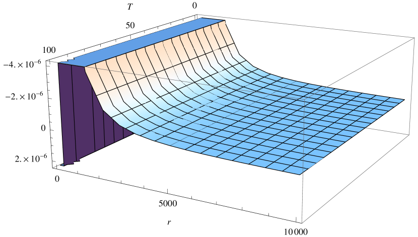
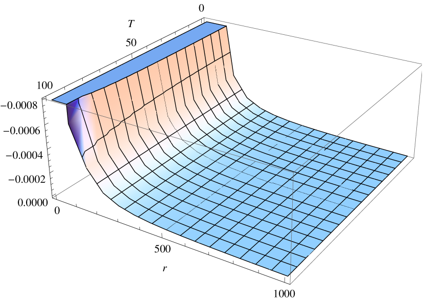
Figure 1: Plot of the dynamical variable $\tilde{Y}_{T}$ for the strange star candidate 4U 1820-30.

Figure 2: Behavior of the dynamical variable $\tilde{X}_{T}$ for the strange star candidate 4U 1820-30.

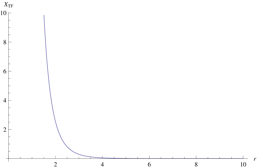
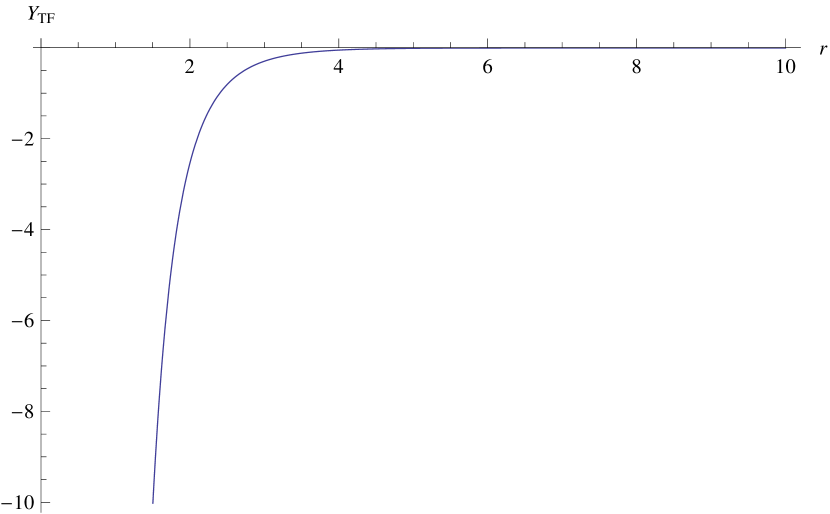
Figure 3: Role of the dark dynamical variable $\tilde{X}_{TF}$ on the evolution of the strange star candidate 4U 1820-30.

Figure 4: Plot for the dark dynamical variable $\tilde{Y}_{TF}$ on the evolution of the strange star candidate 4U 1820-30.

The study of compact objects is amongst the most burning issues of our mysterious dark universe in which, stars came into being during the dying phenomenon of relativistic massive stars. Such celestial bodies are having size as a big city and generally contain mass atleast 40% more mass than solar mass. Due to this fact, their core density exceeds the density of an atomic nucleus. This specifies that the compact stars could be treated as test particle to study some physical features beyond nuclear density.

Rossi X-ray Timing Explorer gathered information based on satellite observations about the structure of a neutron star, named 4U1820-30. They found mass of this star to be $2.25M_{\odot}$ containing high amount of exotic matter. We now apply our results of dynamical dark variables on the observational values of this compact star. As our $f(R,T)$ field equations are non-linear in nature, therefore we suppose that our star consists of non-interacting particles. We suppose that our geometry is demarcated with the three-dimensional boundary surface. The interior to that is given by (3), while the exterior vacuum geometry is given by

$$ds^{2}_{+}=-Z^{2}d\nu^{2}+Z^{-1}d\rho^{2}+\rho^{2}(d\theta^{2}+\sin^{2}{\theta}d\phi^{2}).$$ (43)

where $Z=\left(1-\frac{2M}{\rho}\right)$ with $M$ and $\nu$ are total matter content and retarded time, respectively. We use Darmois junction conditions [49] to make continuous connections between Eqs.(3) and (43) over hypersurface. These conditions, after some manipulations, provide

$$Adt\overset{\Sigma}{=}d\nu\left(1-2\frac{M}{\rho}\right),\quad C\overset{\Sigma}{=}\rho(\nu),$$ (44)

$$M\overset{\Sigma}{=}m(t,r),$$ (45)

These constraints should be fulfilled by both manifolds in order to remove jumps over the boundary.

It is well-known from the literature that the dynamical variable, $Y_{T}$ has the same role as that of the Tolman mass density in the evolutionary phases of those relativistic systems which are in the state of equilibrium or quasi-equilibrium. Figures (2) and (2) state the evolution of $\tilde{Y_{T}}$ and $\tilde{X_{T}}$ variables with the increase of $r$ and $T$, respectively. Other very important dark scalar functions are $\tilde{X_{TF}}$ and $\tilde{Y_{TF}}$. These two variables have opposite behaviors on the dynamical phases of our relativistic 4U 1820-30 star candidate. The modified structure scalar $\tilde{X_{TF}}$ is controlling appearance of inhomogeneities on the initially regular compact object. It can be observed from the Figure (4) that the inhomogeneity of the compact star keep on decreasing by increasing the radial coordinate of the spherical self-gravitating object. The totally reverse behavior of $Y_{TF}$ can be observed from Figure (4).

5 Conclusions

This paper is devoted to explore the effects of extra curvature ingredients of $f(R,T)$ gravity theory on the dynamical variables of compact spherical star. The matter contents in the stellar interior are taken to be imperfect due to anisotropic stresses, shear viscosity and dissipative terms. A particular form of $f(R,T)$ function i.e., $f(R,T)=f_{1}(R)+f_{2}(R)f_{3}(T)$, is utilized to explore the modified field equations. The Misner-Sharp mass function is generalized by including the higher curvature ingredients of $f(R,T)$ theory. We have disintegrated the Weyl tensor, which describes the distortion in the shapes of celestial objects due to tidal forces, in to two parts named as its electric and magnetic parts. The magnetic part vanishes due to the symmetry of spherical star and all the tidal effects are due to its electric component.

A correspondence between the the scalar component associated with Weyl tensor with matter variables has been established under the influence of extra curvature ingredients of $f(R,T)$ theory. In a similar way, we have extracted the electric part of Riemann tensor and formulate its second dual tensor. These couple of tensors are furthers divided into their constituent scalar parts named as structure scalars. These scalar parts are written in terms of matter variables with the help of modified field equations and Weyl scalar. The effects of higher order terms is also found in the formation of these dynamical equations as obtained in Eqs.(27)-(30). These structural dynamical equations have enough significance to discuss the evolution of self-gravitating compact objects. We have also explored the Raychaudhuri equations for shear and expansion scalar which are related with some of the structure scalars. Further, a differential equation is formulated by adopting the procedure developed by Ellis which have importance in the discussion of the inhomogeneous density distribution in the universe. One can find that the irregularities in the matter density can be controlled via one of the scalar variable. We have also explored the dark dynamical variables under the condition of constant Ricci invariant and trace of stress energy tensor. These dark dynamical variables are effected by the tidal effects coming due to the electric part of Weyl tensor. Further, the evolution equations for shear and expansion are formulated in this background and linked with structure scalars. All our results are consistent with those already obtained in the literature.

References

• [1] S. Perlmutter et al., Astrophys. J. 517, 565 (1999).
• [2] A. G. Riess et al., Astron. J. 695, 98 (2007).
• [3] E. Komatsu et al., Astrophys. J. Suppl. 192, 18 (2011).
• [4] T. P. Sotirou and V. Faraoni, Rev. Mod. Phys. 82, 451 (2010).
• [5] S. Capozziello and M. D. Laurentis, Phys. Rep. 509, 167 (2011).
• [6] A. D. Felice and S. Tsujikawa, Living Rev. Relativ. 13, 3 (2010).
• [7] S. Nojiri and S. D. Odintsov, Phys. Rep. 505, 59 (2011) [arXiv:1011.0544 [gr-qc]]
• [8] S. Nojiri and S. D. Odintsov, eConf C 0602061, 06 (2006) [Int. J. Geom. Meth. Mod. Phys. 4, (2007) 115] [hep-th/0601213].
• [9] T. Harko, F. S. N. Lobo, S. Nojiri and S. D. Odintsov, Phys. Rev. D 84, 024020 (2011).
• [10] M. J. S. Houndjo, Int. J. Mod. Phys. D 21, 1250003 (2012).
• [11] E. H. Baffou, A. V. Kpadonou, M. E. Rodrigues, M. J. S. Houndjo and J. Tossa, Astrophys. Space Sci. 356, 173 (2014).
• [12] K.Β Bamba, S.Β Capozziello, S.Β Nojiri and S.Β D.Β Odintsov, Astrophys.Β Space Sci. 342, 155 (2012).
• [13] R. Durrer and R. Maartens, arXiv:0811.4132 [astro-ph].
• [14] S. Capozziello, M. De Laurentis, I. De Martino, M. Formisano and S. D. Odintsov, Phys. Rev. D 85 044022, (2012) [arXiv: 1112.0761].
• [15] S. Capozziello, M. De Laurentis, S. D. Odintsov and A. Stabile Phys. Rev. D 83, 064004 (2011) [arXiv: 1101.0219 [gr-qc]].
• [16] K. Bamba, S. Nojiri and S. D. Odintsov, Phys. Lett. B 698, 451 (2011) [arXiv: 1101.2820].
• [17] M. Sharif and Z. Yousaf, Eur. Phys. J. C 75, 58 (2015); M.Β Z.Β Bhatti,Β Z.Β YousafΒ andΒ S.Β Hanif,Β Mod.Β Phys.Β Lett.Β AΒ 32,Β 1750042Β (2017); Phys. Dark Universe 75, 58 (2017).
• [18] M. Sharif and Z. Yousaf, Eur. Phys. J. C 75, 194 (2015) [arXiv:1504.04367v1 [gr-qc]]; M. Sharif and Z. Yousaf, Astrophys. Space Sci. 355, 317 (2015); Z. Yousaf, K. Bamba and M. Z. Bhatti, Phys. Rev. D 93, 064059 (2016) [arXiv1603.03175 [gr-qc]]; Z. Yousaf, M. Z. Bhatti and U. Farwa, Mon. Not. R. Astron. Soc. 464, 4509 (2017); M. Z. Bhatti, Eur. Phys. J. Plus 131, 428 (2016); Z. Yousaf, Eur. Phys. J. Plus 132, 71 (2017); Eur. Phys. J. Plus 132, 276 (2017); Z.Β Yousaf,Β M.Β Z.Β Bhatti and A. Rafaqat,Β Astrophys. Space Sci. 68, 362 (2017).
• [19] M. Sharif and Z. Yousaf, Astrophys. Space Sci. 357, 49 (2015); Z. Yousaf and M. Z. Bhatti, Mon. Not. R. Astron. Soc. 458, 1785 (2016) [arXiv:1612.02325 [physics.gen-ph]]; Z. Yousaf and M. Z. Bhatti, Eur. Phys. J. C 76, 267 (2016) [arXiv:1604.06271 [physics.gen-ph]].
• [20] P. H. R. S. Moraes, J. D. V. ArbaΓ±il and M. Malheiro, J. Cosmol. Astropart. Phys. 06, 005 (2016).
• [21] L. Herrera, A. Di Prisco, G. Le Denmat, M. A. H. MacCallum and N. O. Santos, Phys. Rev. D 76, 064017 (2007).
• [22] L. Herrera and N. O. Santos, Class. Quantum Grav. 22, 2407 (2005).
• [23] B. C. Tewari, K. Charan and J. Rani, Int. J. Astron. Astrophys. 6, 155 (2016).
• [24] M. Sharif and M. Z. Bhatti, Astropart. Phys. 56, 35 (2014).
• [25] M. Sharif and Z. Yousaf, Astrophys. Space Sci. 354, 471 (2014).
• [26] M. Sharif and Z. Yousaf, Int. J. Theor. Phys. 55, 470 (2016).
• [27] Z. Yousaf, M. Z. Bhatti and U. Farwa, Eur. Phys. J. C 77, 359 (2017).
• [28] Z. Yousaf, M. Z. Bhatti and U. Farwa, Class. Quantum Grav. 34, 145002 (2017).
• [29] R. Penrose and S. W. Hawking, General Relativity, An Einstein Centenary Survey, Cambridge University Press, Cambridge (1979).
• [30] L. Herrera, A. Di Prisco, J. L. HernΓ‘ndez-Pastora and N. O. Santos, Phys. Lett. A 237, 113 (1998).
• [31] K. S. Virbhadra, D. Narasimha, and S. M. Chitre, Astron. Astrophys. 337, 1 (1998); K. S. Virbhadra and G. F. R. Ellis, Phys. Rev. D 65, 103004 (2002).
• [32] K. S. Virbhadra, Phys. Rev. D 79, 083004 (2009).
• [33] L. Herrera, A. Di Prisco, J. Martin, J. Ospino, N. O. Santos and O. Troconis, Phys. Rev. D 69, 084026 (2004).
• [34] L. Herrera, A. Di Prisco and J. IbÑñez, Phys. Rev. D 84, 107501 (2011).
• [35] Z.Β Yousaf,Β K.Β BambaΒ andΒ M.Β Z.Β Bhatti,Β Phys. Rev. D 93, 124048 (2016) [arXiv:1606.00147 [gr-qc]].
• [36] M. Z. Bhatti and Z. Yousaf, Eur. Phys. J. C 76, 219 (2016) [arXiv1604.01395 [gr-qc]]; M. Z. Bhatti and Z. Yousaf, Int. J. Mod. Phys. D 26, 1750029 (2017).
• [37] L. Herrera, A. Di Prisco and J. IbaΓ±ez, Phys. Rev. D 84, 064036 (2011).
• [38] L. Herrera, Entropy 19, 110 (2017) [arXiv:1703.03958 [gr-qc]].
• [39] Z.Β Yousaf,Β K.Β BambaΒ andΒ M.Β Z.Β Bhatti,Β Phys. Rev. D 95, 024024 (2017) [arXiv:1701.03067 [gr-qc]].
• [40] L. Herrera, J. Phys. Conf. Ser. 831, 012001 (2017) [arXiv:1704.04386 [gr-qc]].
• [41] M. J. S. Houndjo and O. F. Piattella, Int. J. Mod. Phys. D 21, 1250024 (2012).
• [42] S. Nojiri and S. D. Odintsov, Phys. Rev. D 68, 123512 (2003).
• [43] C. W. Misner and D. Sharp, Phys. Rev. 136, B571 (1964).
• [44] L. Bel, Ann. Inst. H PoincarΓ© 17, 37 (1961).
• [45] M. Sharif and M. Z. Bhatti, Int. J. Mod. Phys. D 23, 1450085 (2014); Int. J. Mod. Phys. D 24, 1550014 (2015); Mod. Phys. Lett. A 29, 1450165 (2014); 29, 1450094 (2014); M. Sharif and Z. Yousaf, Astrophys. Space Sci. 352, 321 (2015); Astrophys. Space Sci. 354, 481 (2014); Astrophys. Space Sci. 357, 49 (2015); Eur. Phys. J. C 75, 194 (2015); Can. J. Phys. 93, 905 (2015).
• [46] F. D. Albareti, J. A. R. Cembranos, A. de la Cruz-Dombriz and A. Dobado, J. Cosmol. Astropart. Phys. 03, 012 (2014).
• [47] L. Herrera, J. Ospino, A. Di Prisco, E. Fuenmayor and O. Troconis, Phys. Rev. D 79, 064025 (2009).
• [48] L. Herrera, N. O. Santos, and A. Wang, Phys. Rev. D 78, 084026 (2008); L. Herrera, G. Le Denmat, and N. O. Santos, Phys. Rev. D 79, 087505 (2009); M. Sharif and Z. Yousaf, Phys. Rev. D 88, 024020 (2013).
• [49] G. Darmois, Memorial des Sciences Mathematiques (Gautheir-Villars, 1927) Fasc. 25.