A modularity based spectral method for simultaneous community and anti-community detection

Abstract

In a graph or complex network, communities and anti-communities are node sets whose modularity attains extremely large values, positive and negative, respectively. We consider the simultaneous detection of communities and anti-communities, by looking at spectral methods based on various matrix-based definitions of the modularity of a vertex set. Invariant subspaces associated to extreme eigenvalues of these matrices provide indications on the presence of both kinds of modular structure in the network. The localization of the relevant invariant subspaces can be estimated by looking at particular matrix angles based on Frobenius inner products.

1 Introduction

This paper addresses the problem of grouping nodes of a network into communities and anti-communities, possibly emerging from a neutral background. A community is roughly defined as a set of nodes being highly connected inside and poorly connected with the rest of the graph. Conversely, an anti-community is a node set being loosely connected inside but having many external connections. Revealing these structures in data and networks is a challenging and relevant problem which has applications in many disciplines, ranging from computer science to physics and several natural and social sciences [3, 6, 14, 16, 17].

In order to address this problem from the mathematical point of view one needs a quantitative definition of what a community and an anti-community is. To this end several merit functions have been introduced in the recent literature. A very popular and fruitful idea is based on the concept of modularity, originally introduced for community detection in the statistical mechanics literature [18, 19]. The modularity measure of a set of nodes $S\subset V$ in a graph $G=(V,E)$ quantifies the difference between the actual weights of edges in $S$ with respect to the expected weight, if edges were placed at random according to a prescribed null model. The modularity-based criterion for community detection thus identifies a subset $S$ as a community if its modularity measure is “large”, and as an anti-community if its modularity measure is “small”. The (anti-)community detection problem thus boils down to a combinatorial optimization problem, whose solution is typically approximated through a matrix-based technique which exploits the spectrum of a suitably defined modularity matrix.

In this work we show that dominant eigenvalues of generalized modularity matrices can be used to simultaneously look for communities and anti-communities. We propose a spectral method based on the eigenspaces associated with those eigenvalues and relate its performance to certain matrix angles. We then analyze the stochastic block model, one of the most useful generative models in community detection, to obtain indications on the average performance of the proposed method. To that goal, we characterize the dominant eigenvalues and eigenvectors of the average modularity matrix in the model. A couple of numerical experiments are included to validate the proposed computational strategy.

1.1 Notations and preliminaries

In the sequel we give a brief review of standard concepts and symbols from algebraic graph theory that we will use throughout the paper. We assume that $G=(V,E)$ is a finite, undirected graph where $V$ and $E$ are the vertex and edge sets, respectively. We will identify $V$ with $\{1,\dots,n\}$. We denote adjacency of vertices $i$ and $j$ as $ij\in E$. We allow positive weights on both the vertex and the edge sets which we denote by $\mu:V\to\mathbb{R}_{+}$, $i\mapsto\mu(i)$ and $w:E\to\mathbb{R}_{+}$, $ij\mapsto w_{ij}$, respectively.

The symbol $A$ denotes the adjacency matrix of $G$, that is, $A=(a_{ij})$ where $a_{ij}=w_{ij}$ if $ij\in E$, and $a_{ij}=0$ otherwise. In particular, $A$ is a symmetric, componentwise nonnegative matrix. The (generalized) degree of vertex $i\in V$ is $d_{i}=\sum_{j=1}^{n}w_{ij}$, and $\mathbbm{1}$ denotes an all-one vector whose dimension depends on the context. With this notation, the degree vector is $d=A\mathbbm{1}$.

The subgraph induced by a set $C\subseteq V$ is the graph $G(C)$ whose adjacency matrix is the submatrix of $A$ whose row and column indices are in $C$. The cardinality of $C$ is denoted by $|C|$, and its weight by $\mu(C)=\sum_{i\in C}\mu(i)$. For consistency with other works by various authors, a special notation is reserved for the case $\mu(i)=d_{i}$ where we write $\mathrm{vol}(C)=\sum_{i\in C}d_{i}$ for the volume of $C$. Correspondingly, $\mathrm{vol}(V)=\sum_{i\in V}d_{i}$ denotes the volume of the whole graph. Moreover, we denote by $\overline{C}$ the complement $V\setminus C$, and let $\mathbbm{1}_{C}$ be its characteristic vector, defined as $(\mathbbm{1}_{C})_{i}=1$ if $i\in C$ and $(\mathbbm{1}_{C})_{i}=0$ otherwise, so that $\mathrm{vol}(C)=\mathbbm{1}_{C}^{T}d$.

The Frobenius inner product of two matrices $A,B\in\mathbb{R}^{n\times n}$ is $\langle A,B\rangle=\mathrm{trace}(A^{T}B)$, and the associated matrix norm is $\|A\|_{\mathrm{F}}=\langle A,A\rangle^{1/2}$. For later reference, we recall the Hoffman–Wielandt theorem for singular values and the Eckart–Young theorem, see e.g., [13, 21].

Theorem 1.1 (Hoffman–Wielandt).

Let $A$ and $B$ be two $n\times n$ matrices. Denote by $s_{i}(A)$ and $s_{i}(B)$ their singular values arranged in nonincreasing order. Then

$$\sum_{i=1}^{n}(s_{i}(A)-s_{i}(B))^{2}\leq\|A-B\|_{\mathrm{F}}^{2}.$$

Theorem 1.2 (Eckart–Young).

Let $A=U\Lambda U^{T}$ be a symmetric matrix with eigenvalues arranged in nonincreasing modulus, $|\lambda_{1}|\geq|\lambda_{2}|\geq\ldots\geq|\lambda_{n}|$. For any integer $1\leq k\leq n$ let $A_{k}=U_{k}\Lambda_{k}U_{k}^{T}$ where $U_{k}$ is the $n\times k$ matrix formed by the first $k$ columns of $U$ and $\Lambda_{k}=\mathrm{Diag}(\lambda_{1},\ldots,\lambda_{k})$. Then

$$\|A-A_{k}\|_{\mathrm{F}}^{2}=\min_{\mathrm{rank}(B)\leq k}\|A-B\|_{\mathrm{F}}^{2}=\textstyle{\sum_{i=k+1}^{n}\lambda_{i}^{2}}.$$

1.2 Matrix projections and angles

Let $\mathcal{S}$ be a linear subspace of $\mathbb{R}^{n\times n}$. The orthogonal projection of a matrix $A$ onto $\mathcal{S}$ with respect to the Frobenius inner product is

$$P=\mathcal{P}(A,\mathcal{S})\quad\Longleftrightarrow\quad\|A-P\|_{\mathrm{F}}=\min_{B\in\mathcal{S}}\|A-B\|_{\mathrm{F}}.$$

Furthermore, we define the angle between $A$ and $\mathcal{S}$ through the trigonometric functions

$$\sin(A,\mathcal{S})=\frac{\|A-P\|_{\mathrm{F}}}{\|A\|_{\mathrm{F}}},\qquad\cos(A,\mathcal{S})=\frac{\|P\|_{\mathrm{F}}}{\|A\|_{\mathrm{F}}},$$

where $P=\mathcal{P}(A,\mathcal{S})$.

For any fixed integer $1\leq k\leq n-1$ let $\mathbb{O}^{n\times k}$ be the set of all $n\times k$ matrices with orthonormal columns. For any $X=[x_{1},\ldots,x_{k}]\in\mathbb{O}^{n\times k}$ we denote by $\mathcal{H}(X)$ the matrix subspace

$$\mathcal{H}(X)=\left\{H=\sum_{i=1}^{k}\tau_{i}x_{i}x_{i}^{T},\tau_{i}\in\mathbb{R}\right\}.$$

Equivalently, any matrix in $\mathcal{H}(X)$ admits the factorization $XTX^{T}$ where $T=\mathrm{Diag}(\tau_{1},\ldots,\tau_{k})$. Simple arguments produce the explicit expression

$$\mathcal{P}(A,\mathcal{H}(X))=\sum_{i=1}^{k}\tau_{i}x_{i}x_{i}^{T},\qquad\tau_{i}=x_{i}^{T}Ax_{i}.$$

Moreover, we denote by $\mathcal{K}(X)$ the matrix subspace

$$\mathcal{K}(X)=\left\{K=XSX^{T},\ S=S^{T}\in\mathbb{R}^{k\times k}\right\}.$$ (1)

Equivalently, $K\in\mathcal{K}(X)$ if and only if $X^{T}KX$ is a symmetric $k\times k$ matrix. Note that $\mathcal{H}(X)\subset\mathcal{K}(X)$. Simple arguments produce the explicit expression

$$\mathcal{P}(A,\mathcal{K}(X))=XX^{T}AXX^{T}.$$

The following result is an easy consequence of the Eckart–Young theorem; we omit the simple proof, which is based on the fact that, for arbitrary $X\in\mathbb{O}^{n\times k}$, both $\mathcal{H}(X)$ and $\mathcal{K}(X)$ describe the set of all $n\times n$ symmetric matrices with rank not larger than $k$.

Theorem 1.3.

Let $A=U\Lambda U^{T}$ be a symmetric matrix with eigenvalues arranged in nonincreasing modulus, $|\lambda_{1}|\geq|\lambda_{2}|\geq\ldots\geq|\lambda_{n}|$. For any fixed integer $1\leq k\leq n-1$, suppose that $|\lambda_{k}|>|\lambda_{k+1}|$. Let $X_{H},X_{K}\in\mathbb{O}^{n\times k}$ be solutions of the variational problems

$$\max_{X\in\mathbb{O}^{n\times k}}\cos(A,\mathcal{H}(X)),\qquad\max_{X\in\mathbb{O}^{n\times k}}\cos(A,\mathcal{K}(X)),$$

respectively. Then there exist orthogonal matrices $Z_{1},Z_{2}\in\mathbb{R}^{k\times k}$ such that

$$U_{k}=X_{H}Z_{1}=X_{K}Z_{2},$$

where $U_{k}\in\mathbb{O}^{n\times k}$ is formed by the first $k$ columns of $U$. In both cases, the projection of $A$ onto the respective spaces is $A_{k}=U_{k}\Lambda_{k}U_{k}^{T}$ where $\Lambda_{k}=\mathrm{Diag}(\lambda_{1},\ldots,\lambda_{k})$.

2 Communities and anti-communities

Discovering the presence of communities in a network is a central problem in data analysis and modern network science. Although there is no clear-cut definition of what a community is, common sense suggests that a set of nodes can be recognized as a community inside a given network if those nodes are tightly connected internally, and loosely connected with the surrounding ones. A rather successful formalization of this informal argument is originally due to Newman and Girvan [19], who proposed a specific measure, called modularity, to quantify the “strength” of a set of nodes as a community. Such measure is based on the argument that $C\subseteq V$ can be recognized as a community if the subgraph induced by $C$ contains more edges than expected, if edges were placed at random according to a certain random graph model. A very noticeable example is the Newman–Girvan modularity, which is defined for any $C\subseteq V$ as

$$Q(C)=\mathbbm{1}_{C}^{T}\widehat{M}\mathbbm{1}_{C},\qquad\widehat{M}=A-dd^{T}\!/\mathrm{vol}(V).$$ (2)

Here, $\mathbbm{1}_{C}^{T}A\mathbbm{1}_{C}$ quantifies the overall weight of edges internal to the subgraph $G(C)$ while $(\mathbbm{1}_{C}^{T}d)^{2}/\mathrm{vol}(V)$ is an a priori estimate of the former quantity according to the so-called Chung–Lu random graph model [4]. The Newman–Girvan modularity enjoys nice properties, for example $Q(C)=Q(\overline{C})$, and $Q(V)=0$. We point the reader to [7] for an extensive analysis of spectral properties of that matrix $\widehat{M}$.

A number of different variants of the modularity measure have been considered afterwards, see e.g., [1, 8, 23, 25]. All of them can be expressed as $\mathbbm{1}_{C}^{T}\widehat{M}\mathbbm{1}_{C}$ by means of a suitably defined (generalized) modularity matrix $\widehat{M}$. Within this setting, the detection of $k$ largest communities in a prescribed network, or the partitioning of its vertex set into $k$ pairwise disjoint communities translates naturally into the maximization of $\sum_{i=1}^{k}Q(C_{i})$ under appropriate conditions on the family $\mathcal{C}=\{C_{1},\ldots,C_{k}\}$. A major alternative formulation is related to normalized versions of the modularity,

$$q(C)=Q(C)/\mu(C)$$ (3)

where $Q(C)$ is as before and $\mu(C)$ is an additive measure of the set $C$, which is used as a balancing function to promote small node groups. The two most common measures are $\mu(C)=|C|$ and $\mu(C)=\mathrm{vol}(C)$, see e.g., [1]. The use of the normalized modularity $q(C)$ has several advantages because of its more reliable underlying algebraic structure and its ability to localize small communities, despite the known tendency of the standard (unnormalized) modularity measures to overlook small groups [10, 25]. We also mention that the normalization term $\mu(C)=\tau|C|+\mathrm{vol}(C)$ has been introduced in a closely related context to cope with sparse networks with strong degree heterogeneity [2, 20]; there, $\tau>0$ is a constant to be tuned in order to minimize the variance of certain statistical estimators.

Besides communities, another subgraph-level structure of interest in network analysis is that of anti-communities. Probably, the first occurrence of the term “anti-community” can be traced back to [18] with reference to vertex sets having $Q(C)\ll 0$. Roughly speaking, a set of nodes is said to have an anti-community structure if internal connections are fewer than those expected by chance. According to [3], in an anti-community nodes have most of their connections outside their group and have no or fewer connections with the members within the same group. For example, an almost bipartite graph (a bipartite graph possibly containing a few erroneous edges) is made of two anti-communities. These informal definitions can be suitably formalized by means of modularity concepts. Actually, the detection of a bipartite structure in a given graph with vertex set $V$ can be handled by the minimization of the Newman–Girvan modularity over subsets of $V$; owing to the equality $Q(C)=Q(\overline{C})$, if $C$ is a set of minimum modularity then $\{C,\overline{C}\}$ gives the bipartite structure of the graph. In fact, if the subgraph induced by $C$ contains no edges, then $\mathrm{vol}(C)=\mathrm{vol}(\overline{C})=\mathrm{vol}(V)/2$ and

$$Q(C)=-\mathrm{vol}(C)^{2}/\mathrm{vol}(V)=-\mathrm{vol}(V)/4,$$

which is the lower bound for $Q$. Further, literature concerned with anti-community structures addresses both the detection of almost-bipartitiveness, see e.g., [18, 22], and the presence of multiple, possibly overlapping anti-communities [1, 3, 6, 17].

In the present work we address the problem of detecting simultaneously the presence of communities and anti-communities in a given network. To that goal, we extend the spectral approach that has been adopted by various authors in community or anti-community detection, as mentioned above. Henceforth, we agree that a node set $C\subset V$ is an anti-community if $q(C)<0$ and “large” (compared to other subsets), and a module if $q(C)^{2}$ is “large”, where $q(C)$ is a normalized modularity function as in (3).

3 Modularity-based detection of communities and anti-communities

Hereafter, we consider the following framework: we are given a (generalized) modularity matrix $\widehat{M}$ such that $Q(C)=\mathbbm{1}_{C}^{T}\widehat{M}\mathbbm{1}_{C}$ and the diagonal matrix $W=\mathrm{Diag}(\mu(1),\ldots,\mu(n))$. To any subset $C\subseteq V$ we associate the measure vector $\chi_{C}$ defined as

$$\chi_{C}=W^{1/2}\mathbbm{1}_{C}/\|W^{1/2}\mathbbm{1}_{C}\|_{2}.$$

Consequently we have $\chi_{C}^{T}\chi_{C}=1$ and

$$\chi_{C}^{T}M\chi_{C}=q(C),\qquad M=W^{-1/2}\widehat{M}W^{-1/2}.$$

Example 3.1.

Let $Q(C)$ be the Newman–Girvan modularity (2).

• If $\mu(j)=1$ for all $j$ then $M=\widehat{M}$, $\chi_{C}=\mathbbm{1}_{C}/|C|^{1/2}$ and

  $$q(C)=\frac{\mathbbm{1}_{C}^{T}\widehat{M}\mathbbm{1}_{C}}{|C|}=\frac{Q(C)}{|C|};$$

• if $\mu(j)=d_{j}$ then $\chi_{C}=W^{1/2}\mathbbm{1}_{C}/\mathrm{vol}(C)^{1/2}$ and $q(C)=Q(C)/\mathrm{vol}(C)$.

A statistics based scrutiny of these two “penalized” versions of $Q(C)$ has been carried out in [1].

Consider a family $\mathcal{C}=\{C_{1},\ldots,C_{k}\}$ of pairwise disjoint subsets of $V$ with $\cup_{i=1}^{k}C_{i}\subseteq V$, and let $X=[\chi_{1},\ldots,\chi_{k}]\in\mathbb{O}^{n\times k}$ where $\chi_{i}$ is the measure vector of $C_{i}$. The problem of recognizing the $k$ largest modules in $G$ can be obviously stated as the maximization over all such $\mathcal{C}$ of the quantity

$$\sigma(\mathcal{C})=\sum_{i=1}^{k}q(C_{i})^{2}.$$

Owing to the equivalent expressions

$$\sigma(\mathcal{C})=\sum_{i=1}^{k}(\chi_{i}^{T}M\chi_{i})^{2}=\|\mathcal{P}(M,\mathcal{H}(X))\|_{\mathrm{F}}^{2}=\|M\|_{\mathrm{F}}^{2}\cos(M,\mathcal{H}(X))^{2},$$

a continuous relaxation of that combinatorial problem consists of computing

$$X^{*}=\mathrm{arg}\max_{X\in\mathbb{O}^{n\times k}}\cos(M,\mathcal{H}(X)).$$ (4)

As recalled in Theorem 1.3, any solution of (4) is related to the $k$ “dominant” eigenvectors of $M$. In fact, given the spectral decomposition $M=U\Lambda U^{T}$ with $U=[u_{1},\dots,u_{n}]$, consider the eigenvalues of $M$ in nonincreasing moduli:

$$|\lambda_{1}|\geq|\lambda_{2}|\geq\cdots\geq|\lambda_{n}|.$$ (5)

If $|\lambda_{k}|>|\lambda_{k+1}|$ then any solution $X^{*}$ of (4) is an orthogonal transform of $U_{k}=[u_{1},\ldots,u_{k}]$, and the orthogonal projection of $M$ onto $\mathcal{H}(X^{*})$ is

$$H=\mathcal{P}(M,\mathcal{H}(X^{*}))=U_{k}\mathrm{Diag}(\lambda_{1},\ldots,\lambda_{k})U_{k}^{T}.$$

Note that $\|H\|_{\mathrm{F}}^{2}=\sum_{i=1}^{k}\lambda_{i}^{2}$ and $\|M-H\|_{\mathrm{F}}^{2}=\sum_{i=k+1}^{n}\lambda_{i}^{2}$, hence

$$\cos(M,\mathcal{H}(X^{*}))^{2}=\textstyle{(\sum_{i=1}^{k}\lambda_{i}^{2})/(\sum_{i=1}^{n}\lambda_{i}^{2})}.$$ (6)

Thus the presence of a “good” set of $k$ modules is indicated by the presence of $k$ “large” eigenvalues in the spectrum of $M$. Moreover, the subsets $C_{1},\ldots,C_{k}$ can be recovered from $U_{k}$ by virtue of the coincidence of the projections $\mathcal{P}(M,\mathcal{H}(X^{*}))$ and $\mathcal{P}(M,\mathcal{K}(X^{*}))$ as described here below.

Consider the matrix space $\mathcal{K}(X)$ defined in (1) with $X=[\chi_{1},\ldots,\chi_{k}]$. Assuming for the moment that $\cup_{i=1}^{k}C_{i}=V$, any matrix in that space has the following block structure, up to a row and column renumbering:

$$K=K^{T}=\begin{pmatrix}K_{11}&\cdots&K_{1k}\\ \vdots&\vdots&\vdots\\ K_{k1}&\cdots&K_{kk}\end{pmatrix}.$$

Here, block $K_{ij}$ has order $|C_{i}|\times|C_{j}|$ and rank one. In fact, let $S=X^{T}KX=(s_{ij})$ and denote by $\hat{\chi}_{i}$ the nonzero part (i.e., the support) of $\chi_{i}$. Then, $K_{ij}=s_{ij}\hat{\chi}_{i}\hat{\chi}_{j}^{T}$. For example, if $\chi_{i}=\mathbbm{1}_{C_{i}}/\sqrt{|C_{i}|}$ then $K_{ij}=(s_{ij}/\sqrt{|C_{i}||C_{j}|})\mathbbm{1}\mathbbm{1}^{T}$. Moreover, given the spectral decomposition $S=Y^{T}DY$ where $Y=[y_{1},\ldots,y_{k}]$ is orthogonal, the matrix $K$ admits the spectral factorization

$$K=XY^{T}DYX^{T}.$$

The matrix of eigenvectors relative to nonzero eigenvalues of $K$ can be partitioned as follows:

$$XY^{T}=\begin{pmatrix}\hat{\chi}_{1}y_{1}^{T}\vspace{2mm}\\ \hat{\chi}_{2}y_{2}^{T}\vspace{2mm}\\ \vdots\vspace{2mm}\\ \hat{\chi}_{k}y_{k}^{T}\end{pmatrix}\begin{array}[]{c}\big{\}}|C_{1}|\vspace{2mm}\\ \big{\}}{\tiny|C_{2}|\vspace{2mm}}\\ \vdots\vspace{2mm}\\ \big{\}}|C_{k}|\end{array}$$

that is, rows with indices in the same $C_{i}$ are parallel, while rows belonging to different $C_{i}$’s are orthogonal. In particular, if $i\in C_{j}$ then the norm of the $i$-th row is $\sqrt{\mu(i)/\mu(C_{j})}$, so that scaling that row by $1/\sqrt{\mu(i)}$ makes the norm depend only on the block index $j$. Thus the partitioning $\mathcal{C}=\{C_{1},\ldots,C_{k}\}$ can be recovered from $XY^{T}$ by clustering its rows according to their angles and lengths. On the other hand, if $\mathcal{C}$ does not cover $V$ then, up to a row renumbering, the block structure of the matrix $K$ above appears in the upper left corner of a larger matrix bordered by null rows and columns. Indeed, in this case $X$ has a trailing block of null rows, which remains unchanged by right-multiplication times orthogonal matrices. Those null rows indicate nodes not belonging to any $C_{i}$’s, while the nonzero rows convey the same information as before.

Clearly, if $\cos(M,\mathcal{H}(X))=1$ then $M\in\mathcal{H}(X)\subseteq\mathcal{K}(X)$, $U_{k}=XY^{T}$ and the modules of $\mathcal{C}$ are inscribed in the rows of $U_{k}$. In a more realistic setting, by a continuity argument if $\cos(M,\mathcal{H}(X))$ does not exactly equal one but is “close to one” then $U_{k}$ can be regarded as a perturbation of $XY^{T}$ in the sense that there is an orthogonal matrix $Z$ such that $U_{k}-XZ$ has small norm. Precise statements can be obtained from Davis–Kahan “$\sin\theta$” theorem [21, Thm. 3.6]; the ensuing Corollary 4.4 provides a result in that spirit.

Hence, a spectral method to locate $k$ “dominant” modules of a given graph or network, possibly not covering the whole vertex set, can be based on the computation of $k$ extreme eigenpairs of $M$, and the use of a clustering algorithm to group rows of $U_{k}$ according to their position in $\mathbb{R}^{k}$. For that task, a popular idea in the clustering literature is to adopt the $k$-means algorithm, see e.g., [1, 20, 26]. However, since that algorithm always returns a partitioning which covers $V$, we keep in view that the number of disjoint subsets can be equal to the number of considered eigenvalues plus one; the supplemental set can be interpreted as a “background” in the graph from where the dominant modules emerge. This possibility is substantiated in the analysis of the stochastic block model in section 5 and illustrated by a couple of numerical examples in section 6.

4 Analysis of the method

The purpose of this section is to provide theoretical foundation to the foregoing spectral algorithm. In particular, we prove that if the angle between $M$ and $\mathcal{H}(X)$ is “small” then $k$ leading eigenvalues of $M$ are well separated from the others, their values are close to the numbers $q(C_{1}),\ldots,q(C_{k})$, and the span of the corresponding eigenvectors is close to that of $X$. To that goal, we extend the technique introduced in [9] to localize a single dominant eigenvalue of a symmetric matrix.

4.1 Eigenvalues

Equation (6) yields an attainable upper bound on the cosine between $M$ and any space $\mathcal{H}(X)$. In the following theorem we prove a refined upper bound that provides a stronger indication on the dominance of the first $k$ eigenvalues of $M$.

Theorem 4.1.

Let $\{C_{1},\dots,C_{k}\}$ be a family of pairwise disjoint subsets of $V$, ordered so that $|q(C_{1})|\geq\dots\geq|q(C_{k})|$, and let $X=[\chi_{1},\ldots,\chi_{k}]$. Let the eigenvalues of $M$ be denoted as in (5). If $s=\sin(M,\mathcal{H}(X))$ and $c=\cos(M,\mathcal{H}(X))$ then

$$\sum_{i=1}^{k}\lambda_{i}^{2}\geq c^{2}\sum_{i=1}^{n}\lambda_{i}^{2}+\sum_{i=1}^{k}(|\lambda_{i}|-|q(C_{i})|)^{2}.$$

Moreover,

$$\sum_{i=1}^{k}(|\lambda_{i}|-|q(C_{i})|)^{2}\leq s^{2}\sum_{i=1}^{k}\lambda_{i}^{2}.$$

Proof.

Note that the eigenvalues of $H=\mathcal{P}(M,\mathcal{H}(X))$ are the numbers $q(C_{i})$, and the singular values of $M$ and $H$ are the absolute values of their respective eigenvalues. Thus, using Theorem 1.1, we get

$$s^{2}\sum_{i=1}^{n}\lambda_{i}^{2}=s^{2}\|M\|_{\mathrm{F}}^{2}=\|M-H\|_{\mathrm{F}}^{2}\geq\sum_{i=k+1}^{n}\lambda_{i}^{2}+\sum_{i=1}^{k}(|\lambda_{i}|-|q(C_{i})|)^{2}.$$ (7)

With simple manipulations we get

$$\sum_{i=1}^{k}\lambda_{i}^{2}\geq(1-s^{2})\sum_{i=1}^{n}\lambda_{i}^{2}+\sum_{i=1}^{k}(|\lambda_{i}|-|q(C_{i})|)^{2},$$

proving the first claim. Similarly, from (7) we obtain

$$\sum_{i=1}^{k}(|\lambda_{i}|-|q(C_{i})|)^{2}\leq s^{2}\sum_{i=1}^{k}\lambda_{i}^{2}-(1-s^{2})\sum_{i=k+1}^{n}\lambda_{i}^{2}\leq s^{2}\sum_{i=1}^{k}\lambda_{i}^{2}$$

proving the second claim as well. ∎

Remark 4.2.

Simple arguments show the equality

$$\frac{(|\lambda_{i}|-|q(C_{i})|)^{2}}{\lambda_{i}^{2}}=\left|1-\frac{q(C_{i})}{\lambda_{i}}\right|^{2}.$$

Hence, if for $i=1,\dots,k$ we have $|1-q(C_{i})/\lambda_{i}|>s$ then

$$\sum_{i=1}^{k}(|\lambda_{i}|-|q(C_{i})|)^{2}>s^{2}\sum_{i=1}^{k}\lambda_{i}^{2}$$

and the inequality in the last claim of Theorem 4.1 cannot hold. Thus, in the hypotheses of that theorem, for at least some indices $i$ we must have $1-s\leq q(C_{i})/\lambda_{i}\leq 1+s$.

4.2 Eigenspaces

Our next aim is to evaluate quantitatively the closeness of $\chi_{1},\ldots,\chi_{k}$ to the eigenspace associated to the first $k$ eigenvalues of $M$. To quantify the departure of $\mathrm{Range}(X)$ from that eigenspace we resort to a classical metric among subspaces in $\mathbb{R}^{n}$ and a particular inequality in the spirit of Davis–Kahan “$\sin\theta$” theorem [21, Thm. 3.6].

Let $X,Y\in\mathbb{O}^{n\times k}$ and let $\mathcal{X}=\mathrm{Range}(X)$ and $\mathcal{Y}=\mathrm{Range}(Y)$. Recall that the singular values of $X^{T}Y$ are the cosines of the principal angles between $\mathcal{X}$ and $\mathcal{Y}$. These angles quantify the deviation of each subspace from the other. Moreover, if $X_{\perp}$ is an $n\times(n-k)$ matrix such that $[X,X_{\perp}]$ is orthogonal, then the singular values of $X_{\perp}^{T}Y$ are the sines of the same angles. In fact, metrics in the set of all $k$-dimensional subspaces of $\mathbb{R}^{n}$ are usually defined by means of an unitarily invariant matrix norm as $\mathrm{dist}(\mathcal{X},\mathcal{Y})=\|X_{\perp}^{T}Y\|$, see e.g., [21, Thm. 4.9].

Theorem 4.3.

Let $M=U\Lambda U^{T}$ be a spectral decomposition of $M$, and consider the partitioning $U=[U_{1},U_{2}]$ where $U_{1}\in\mathbb{O}^{n\times k}$ is made by unit eigenvectors associated to the $k$ leading eigenvalues of $M$. If $X=[\chi_{1},\ldots,\chi_{k}]$ and $X_{\perp}$ are as before then

$$\|U_{1}^{T}X_{\perp}\|_{\mathrm{F}}^{2}\leq s^{2}\frac{\|M\|_{\mathrm{F}}^{2}}{\lambda_{k}^{2}}-\sum_{i=1}^{k}\frac{\|M\chi_{i}-q(C_{i})\chi_{i}\|_{2}^{2}}{\lambda_{k}^{2}},$$

where $s=\sin(M,\mathcal{H}(X))$.

Proof.

Let $H=\mathcal{P}(M,\mathcal{H}(X))$ and $\Lambda_{1}=U_{1}^{T}MU_{1}=\mathrm{Diag}(\lambda_{1},\ldots,\lambda_{k})$. By construction $HX_{\perp}=O$. Consequently,

$$U_{1}^{T}(M-H)X_{\perp}=U_{1}^{T}MX_{\perp}=\Lambda_{1}U_{1}^{T}X_{\perp}.$$

Moreover,

$$\|(M-H)X_{\perp}\|_{\mathrm{F}}\geq\|U_{1}^{T}(M-H)X_{\perp}\|_{\mathrm{F}}=\|\Lambda_{1}U_{1}^{T}X_{\perp}\|_{\mathrm{F}}\geq|\lambda_{k}|\|U_{1}^{T}X_{\perp}\|_{\mathrm{F}},$$

the last inequality coming from $\|U_{1}^{T}X_{\perp}\|_{\mathrm{F}}\leq\|\Lambda_{1}^{-1}\|_{2}\|\Lambda_{1}U_{1}^{T}X_{\perp}\|_{\mathrm{F}}$. By the orthogonality condition $X^{T}X_{\perp}=O$ we also obtain

$$\|(M-H)X_{\perp}\|_{\mathrm{F}}^{2} =\|M-H\|_{\mathrm{F}}^{2}-\|(M-H)X\|_{\mathrm{F}}^{2}$$

$$=\sin^{2}(M,\mathcal{H}(X))\|M\|_{\mathrm{F}}^{2}-\sum_{i=1}^{k}\|M\chi_{i}-q(C_{i})\chi_{i}\|_{2}^{2}.$$

Collecting all results we complete the proof. ∎

Corollary 4.4.

In the notations of the previous theorem, there exists a $k\times k$ orthogonal matrix $Z$ such that

$$\|U_{1}-XZ\|_{\mathrm{F}}\leq\frac{\sqrt{2}\,\|M\|_{\mathrm{F}}}{|\lambda_{k}|}\sin(M,\mathcal{H}(X)).$$

Proof.

From [21, Thm. 4.11] we get

$$\min_{Z^{T}Z=I}\|U_{1}-XZ\|_{\mathrm{F}}\leq\sqrt{2}\|U_{1}^{T}X_{\perp}\|_{\mathrm{F}},$$

and the claim follows from the previous theorem. ∎

The previous results show that if the angle between $M$ and $\mathcal{H}(X)$ is small then not only $\mathrm{Range}(X)$ is close to $\mathrm{Range}(U_{1})$ but also the residuals $\|M\chi_{i}-q(C_{i})\chi_{i}\|_{2}$ must be small.

5 Modularity analysis of the stochastic block model

A Stochastic Block Model (SBM) with $n$ nodes and $k$ blocks is a random graph model parametrized by the membership matrix $\Theta\in\{0,1\}^{n\times k}$ and the symmetric connectivity matrix $B=(b_{ij})\in\mathbb{R}^{k\times k}$. Every row of the matrix $\Theta$ contains exactly one nonzero entry, whose position indicates which block that node belongs to; and the nonzero entries in the $i$-th column indicate nodes belonging to the $i$-th block. For visual convenience, we assume that each block consists of consecutive integers. The entry $b_{ij}$ is the edge probability between any node in block $i$ and any node in block $j$. Edges are generated independently from one another.

The SBM is one of the most widespread generative models for random graphs and is widely used as a theoretical benchmark for graph partitioning and community detection algorithms, see e.g., [2, 15, 20].

Suppose that the $i$-th block has $n_{i}$ elements, $n_{1}+\cdots+n_{k}=n$. Hence, the average adjacency matrix within the SBM with parameters $(\Theta,B)$ is

$$\overline{A}=\Theta B\Theta^{T}=\begin{pmatrix}\overline{A}_{11}&\cdots&\overline{A}_{1k}\\ \vdots&&\vdots\\ \overline{A}_{k1}&\cdots&\overline{A}_{kk}\end{pmatrix},\qquad\overline{A}_{ij}=b_{ij}\mathbbm{1}\mathbbm{1}^{T}\in\mathbb{R}^{n_{i}\times n_{j}}.$$ (8)

Lemma 5.1.

The average Newman–Girvan modularity matrix (2) of the SBM with parameters $(\Theta,B)$ is

$$\overline{M}=\begin{pmatrix}\overline{M}_{11}&\cdots&\overline{M}_{1k}\\ \vdots&&\vdots\\ \overline{M}_{k1}&\cdots&\overline{M}_{kk}\end{pmatrix},\qquad\overline{M}_{ij}=(b_{ij}-\overline{d}_{i}\overline{d}_{j}/\nu)\mathbbm{1}\mathbbm{1}^{T}\in\mathbb{R}^{n_{i}\times n_{j}},$$

where $\overline{d}=\overline{A}\mathbbm{1}$ and $\nu=\mathbbm{1}^{T}\overline{d}$.

Proof.

By construction, the vector $\overline{d}=\overline{A}\mathbbm{1}$ with $\overline{A}$ given by (8) is the average degree vector for a random graph extracted from the considered model. In particular, if node $i$ belongs to block $\ell$ then $\overline{d}_{i}=\sum_{j=1}^{k}b_{\ell j}n_{j}$. By linearity of the expectation, $\overline{M}=\overline{A}-\overline{d}\,\overline{d}^{T}\!/\nu$ for some scalar $\nu$. Since the equation $M\mathbbm{1}=0$ holds true for every Newman–Girvan modularity matrix, we must set $\overline{M}\mathbbm{1}=0$. That equation produces the value for $\nu$ indicated above, and the proof is complete. ∎

We borrow from [11] the definition of inflation product of two matrices.

Definition 5.2.

Let $A\in\mathbb{R}^{n\times n}$ be a matrix partitioned in $k\times k$ block form, with (nontrivial) square diagonal blocks having possibly different sizes, and let $B=(b_{ij})\in\mathbb{R}^{k\times k}$. The inflation matrix of $B$ with respect to $A$ is the $n\times n$ block matrix

$$B\hbox{$\times\times$}A=\begin{pmatrix}b_{11}A_{11}&\cdots&b_{1k}A_{1k}\\ \vdots&&\vdots\\ b_{k1}A_{k1}&\cdots&b_{kk}A_{kk}\end{pmatrix}.$$

The notation $B\hbox{$\times\times$}A$ does not mention explicitly the partitioning of $A$ on which the result depends; that partitioning should be clear from the context. In this section, we always refer to the block partitioning appearing in (8). Moreover, note that the operator $\times\times$ defined above is a special case of the Khatri–Rao product of two block matrices, see e.g., [13, §12.3.3], and is closely related to the Kronecker product $\otimes$; indeed, when $n_{1}=\ldots=n_{k}=n/k$ and all blocks of $A$ are equal to $Z$ then $B\hbox{$\times\times$}A=B\otimes Z$. For notational convenience, we extend the operator $\times\times$ to vectors as follows: if $w\in\mathbb{R}^{n}$ is a vector partitioned into $k$ (nontrivial) sub-vectors as $w=(w_{1}^{T},\ldots,w_{k}^{T})^{T}$ and $v=(v_{1},\ldots,v_{k})^{T}\in\mathbb{R}^{k}$ then

$$v\hbox{$\times\times$}w=(v_{1}w_{1}^{T},\ldots,v_{k}w_{k}^{T})^{T}\in\mathbb{R}^{n}.$$

The following result is a simple case of more general results shown in Lemma 4.17 and Lemma 4.19 of [11]; we refrain from including the rather technical proof.

Lemma 5.3.

Let $w\in\mathbb{R}^{n}$ be a vector with no zero entries, and let $B\in\mathbb{R}^{k\times k}$ be a symmetric matrix with spectral decomposition $B=V\Lambda V^{T}$ where $V=[v_{1}\ldots,v_{k}]$ and $\Lambda=\mathrm{Diag}(\lambda_{1},\ldots,\lambda_{k})$. Suppose that $w$ is partitioned into $k$ sub-vectors,

$$w=(w_{1}^{T},\ldots,w_{k}^{T})^{T},\qquad w_{i}\in\mathbb{R}^{n_{i}},$$

such that $w_{i}^{T}w_{i}=1$ for $i=1,\ldots,k$. Then

$$B\hbox{$\times\times$}ww^{T}=\sum_{i=1}^{k}\lambda_{i}v_{i}v_{i}^{T}\hbox{$\times\times$}ww^{T}.$$ (9)

Observe that equation (9) is actually a spectral decomposition. Indeed, $v_{i}v_{i}^{T}\hbox{$\times\times$}ww^{T}$ is a rank-one matrix that can be written also as $z_{i}z_{i}^{T}$ with $z_{i}=v_{i}\hbox{$\times\times$}w$; furthermore, $z_{i}^{T}z_{i}=1$ and $z_{i}^{T}z_{j}=0$ for $i\neq j$.

Theorem 5.4.

Let $\overline{M}$ be the average Newman–Girvan modularity matrix of the SBM with parameters $(\Theta,B)$. Let $N=\mathrm{Diag}(n_{1}^{1/2},\ldots,n_{k}^{1/2})$, and let $\delta=(\delta_{1},\ldots,\delta_{k})^{T}$ where $\delta_{i}=\sum_{j=1}^{k}b_{ij}n_{j}$ for $i=1,\ldots,k$. Then the nonzero eigenvalues of $\overline{M}$ coincide with the nonzero eigenvalues of the $k\times k$ matrix

$$N(B-\delta\delta^{T}\!/\nu)N,\qquad\nu=\sum_{i,j}b_{ij}n_{i}n_{j}.$$

Furthermore, let $(\lambda_{i},v_{i})$ be an eigenpair of that matrix and let $z_{i}=N^{-1}v_{i}\hbox{$\times\times$}\mathbbm{1}$. Then $\overline{M}z_{i}=\lambda_{i}z_{i}$.

Proof.

Observe that the number $\delta_{i}$ is the average degree of the nodes belonging to the $i$-th block. In fact, the average degree vector $\overline{d}$ introduced in Lemma 5.1 can be written as $\overline{d}=\delta\hbox{$\times\times$}\mathbbm{1}$. By considering the explicit form of $\overline{M}$ which is given in that lemma, it is not difficult to recognize that $\overline{M}=Z\hbox{$\times\times$}\mathbbm{1}\mathbbm{1}^{T}$ where

$$Z=B-\delta\delta^{T}\!/\nu.$$ (10)

Define $w=(w_{1}^{T},\ldots,w_{k}^{T})^{T}$ where $w_{i}=\mathbbm{1}/n_{i}^{1/2}\in\mathbb{R}^{n_{i}}$ and let $Z=(z_{ij})$. Then, for $i,j=1,\ldots,k$ the block $(i,j)$ of $Z\hbox{$\times\times$}\mathbbm{1}\mathbbm{1}^{T}$ is the $n_{i}\times n_{j}$ matrix

$$z_{ij}\mathbbm{1}\mathbbm{1}^{T}=n_{i}^{1/2}n_{j}^{1/2}z_{ij}w_{i}w_{j}^{T}=(NZN)_{ij}w_{i}w_{j}^{T}=(NZN\hbox{$\times\times$}ww^{T})_{ij},$$

hence $\overline{M}=NZN\hbox{$\times\times$}ww^{T}$. The fist part of the claim follows by a straightforward application of Lemma 5.3. To complete the proof it is sufficient to observe that the $j$-th sub-vector of $z_{i}=v_{i}\hbox{$\times\times$}w_{i}$ is

$$(v_{i}\hbox{$\times\times$}w_{i})_{j}=(v_{i})_{j}\mathbbm{1}/n_{j}^{1/2}=(N^{-1}v_{i})_{j}\mathbbm{1}=(N^{-1}v_{i}\hbox{$\times\times$}\mathbbm{1})_{j}\in\mathbb{R}^{n_{j}}$$

for $j=1,\ldots,k$, hence $z_{i}=N^{-1}v_{i}\hbox{$\times\times$}\mathbbm{1}$ and the proof is complete. ∎

We point out that the matrix $N(B-\delta\delta^{T}\!/\nu)N$ has a nontrivial kernel. Indeed, if $v=(n_{1},\ldots,n_{k})^{T}$ then $Bv=\delta$, $\delta^{T}v=\nu$ and

$$N(B-\delta\delta^{T}\!/\nu)N\mathbbm{1}=N(B-\delta\delta^{T}\!/\nu)v=N(\delta-\delta(\delta^{T}v/\nu))=0.$$

Hence, the matrix $\overline{M}$ for a SBM with $k$ blocks has at most $k-1$ nonzero eigenvalues. This fact suggests that the presence of $k$ “dominant” modules in a SBM graph is indicated by $k-1$ dominant eigenvalues in the spectrum of the modularity matrix. The special case where all those modules have positive modularity (i.e., they are communities) has been considered in Theorem 6.1 of [7].

Remark 5.5.

Let $\Delta=\mathrm{Diag}(\delta_{1},\ldots,\delta_{k})$. Then, $\overline{W}=\Delta\hbox{$\times\times$}I$ is the diagonal matrix of the average degrees in the SBM. By means of arguments completely analogous to the preceding ones, we can also consider the matrix $\widetilde{M}=\overline{W}^{-1/2}\,\overline{M}\,\overline{W}^{-1/2}$ that, within some approximation, can be considered as the average modularity matrix associated to the second case of Example 3.1. The results below are straightforward:

• $\widetilde{M}=\Delta^{-1/2}Z\Delta^{-1/2}\hbox{$\times\times$}\mathbbm{1}\mathbbm{1}^{T}$ where $Z$ is as in (10);

• equivalently, $\widetilde{M}=N\Delta^{-1/2}Z\Delta^{-1/2}N\hbox{$\times\times$}ww^{T}$ where $w$ is as in the proof of Theorem 5.4;

• let $(\lambda_{i},v_{i})$ be an eigenpair of $N\Delta^{-1/2}Z\Delta^{-1/2}N$ and let $z_{i}=N^{-1}v_{i}\hbox{$\times\times$}\mathbbm{1}$. Then $\widetilde{M}z_{i}=\lambda_{i}z_{i}$, and $\widetilde{M}$ has no other nonzero eigenvalues.

Note that the eigenvectors $z_{1},\ldots,z_{k}$ found above of both $\overline{M}$ and $\widetilde{M}$ are constant within each block of the SBM. Consequently, if $\mathcal{C}=\{C_{1},\ldots,C_{k}\}$ covers $V$ and $X=[\chi_{1},\ldots,\chi_{k}]$ then $\cos(\overline{M},\mathcal{H}(X))=\cos(\widetilde{M},\mathcal{H}(X))=1$.

6 Numerical examples

In this section we apply the spectral method discussed so far to the simultaneous search for communities and anti-communities in some real world networks of moderate size. The main aim of the following experimental analysis is to show the effectiveness of the method in recognizing different components of a network being either well inter-connected or well intra-connected, by exploiting the invariant subspace associated to the eigenvalues with largest modulus of the modularity matrix. We do not concern ourselves with implementation details and performance issues.

In the forthcoming experiments we consider graphs with unweighted edges, $w\equiv 1$, and we fix the vertex weight function $\mu\equiv 1$. This leads to the original modularity formulation (2). We locate a small number $k$ of dominant eigenvalues of the modularity matrix that are well separated from the others on the basis of a visual inspection of the spectrum. More precisely, considering the eigenvalues numbered as in (5), we plot the ratios $|\lambda_{i}|/|\lambda_{i+1}|$ for $i=1,\ldots,20$; the index $k$ is chosen by discriminating those ratios that stand out from the others, see Figure 1. Then, we collect the associated eigenvectors in an $n\times k$ matrix; the rows of that matrix are partitioned into $k+1$ groups by means of the Matlab function kmeans, and the resulting clusters are transferred to the original network.

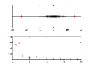
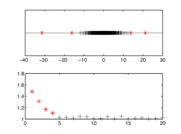
Figure 1: Modularity eigenvalue distributions (top) and ratios $|\lambda_{i}/\lambda_{i+1}|$ (bottom) of two real world networks. Left: Small World citation network. Right: E. Coli protein network. Eigenvalues marked with a red asterisk are considered as relevant.

Small World citation network

The first example we discuss is an instance of the network known as “Small world citation network” where the nodes represent papers that cite the pioneering work of S. Milgram [24] or contain “Small World” in the title, appeared in the period 1967–2003, and edges represent citations. This network contains 233 nodes and 994 oriented edges and is drawn from the Garfield’s collection of citation network datasets produced using the HistCite software [12]. The adjacency matrix, which is freely available in Matlab format from [5], has been symmetrized by neglecting edge orientation. Looking at the two leftmost plots in Figure 1 one clearly recognizes two outliers in the spectrum of the modularity matrix. Thus we embed the nodes into the plane spanned by the eigenvectors associated with the two eigenvalues with largest magnitude and apply $k$-means to partition the node set into three groups, $\mathcal{C}=\{C_{1},C_{2},C_{3}\}$. The method clearly identifies two communities and one anti-community, as shown in Table 1 and Figure 2.

	$C_{1}$	$C_{2}$	$C_{3}$
$|C|$	104	2	127
$Q(C)$	336	$-$30	339
$q(C)$	3.23	$-$15	2.67

Table 1: Size, modularity and normalized modularity values for the sets $C_{1}$, $C_{2}$ and $C_{3}$, located by the spectral method on the Small World citation network.

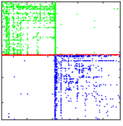
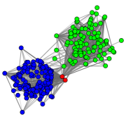
Figure 2: (Best seen in colors) Simultaneous community/anti-community detection on the Small World citation network. Left: colored sparsity pattern (spy) of the adjacency matrix, when the nodes of the network are clustered using the first two eigenvectors of $M$. Right: graph drawing of the communities $C_{1}$ and $C_{3}$ (blue and green) and the anti-community $C_{2}$ (red) located by the method.

E. Coli protein-protein interaction network

The second network shows the interaction between proteins within the Escherichia Coli bacterium. Several instances of this network have been gathered in recent years. Here we consider the dataset from [27] formed by 10788 edges (interactions) between 1251 nodes (proteins). The relative separation of the first $4$ modularity eigenvalues is rather different from that of the bulk of the spectrum, as shown in the rightmost plots in Figure 1, so we set $k=4$ in this example. Using $k$-means to locate a partition into 5 groups, we are able to capture a clear community and anti-community structure in this network. The method locates the partition $\mathcal{C}=\{C_{1},\dots,C_{5}\}$ shown by the colored sparsity patterns in Figure 3. A large portion of the nodes are assigned to a single large community $C_{1}$ (colored in blue) which however has a moderate modularity value $q(C_{1})$ and can be regarded as “background noise”, whereas the remaining nodes are well-clustered into two communities $C_{2}$ and $C_{3}$ (colored in red and green, respectively) and two anti-communities $C_{4}$ and $C_{5}$ (colored in magenta and cyan, respectively). Table 2 shows sizes and modularity scores for the node sets in $\mathcal{C}$, whereas the rightmost plot in Figure 3 provides a qualitative overview of the community/anti-community structure of the most relevant part of the graph.

	$C_{1}$	$C_{2}$	$C_{3}$	$C_{4}$	$C_{5}$
$|C|$	1021	86	60	50	34
$Q(C)$	377	396	289	$-$75	$-$335
$q(C)$	0.36	4.61	4.82	$-$1.51	$-$9.87

Table 2: Size, modularity and normalized modularity values for the sets $C_{1},\dots,C_{5}$, located by the spectral method on the E. Coli protein-protein interaction network.

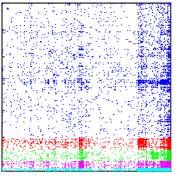
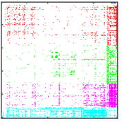
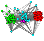
Figure 3: (Best seen in colors) Simultaneous community/anti-community detection on the E. Coli protein-protein interaction network. Left: colored sparsity pattern (spy) of the adjacency matrix, when the nodes of the network are clustered using four dominant eigenvectors of $M$. Center: close-up of the entries of the adjacency matrix corresponding to the four smaller clusters $C_{2},\dots,C_{5}$. Right: graph drawing of the communities $C_{2}$ and $C_{3}$ (red and green) and the anti-communities $C_{4}$ and $C_{5}$ (magenta and cyan) located by the method.

7 Conclusions

Anti-communities are group of nodes showing few internal connections but being highly connected with the rest of the graph. Motivated by a number of data science applications, the interest towards this kind of groups is growing alongside the one for more classical communities.

In this work we propose the use of extremal eigenvalues and eigenvectors of generalized modularity matrices to simultaneously look for non-overlapping group of nodes that are likely to be recognizable as communities or anti-communities in a network. That technique arises as a continuous relaxation of the combinatorial optimization problem of maximizing the sum of squared normalized modularities.

Our approach is not bound to one specific definition of modularity, and allows for different normalization terms. We provide other matrix theoretical evidences of the soundness of the spectral method proposed, together with a detailed analysis of the stochastic block model (SBM). Even though spectral approaches based on Laplacian or adjacency matrices have been proposed in the past for this generative model, the use of generalized modularity matrices in this context has been mostly overlooked. Our analysis together with our final numerical examples, instead, show the effectiveness of this technique on real world data. Furthermore, the machinery we developed for our results can be employed to extend our analysis to the more flexible degree corrected SBM [15, 20] which allows the generation of random graphs having greater degree heterogeneity and may yield a better understanding of the behavior of spectral methods on real world data.

References

- [1] M. Bolla. Penalized versions of the Newman–Girvan modularity and their relation to normalized cuts and K-means clustering. Phys. Rev. E, 84:016108, 2011.
- [2] K. Chaudhuri, F. Chung, and A. Tsiatas. Spectral clustering of graphs with general degrees in the extended planted partition model. In Conference on Learning Theory (COLT), volume 23 of JMLR: Workshop and Conference Proceedings, pages 35:1–35:23, 2012.
- [3] L. Chen, Q. Yu, and B. Chen. Anti-modularity and anti-community detecting in complex networks. Information Sciences, 275:293–313, 2014.
- [4] F. Chung and L. Lu. Complex Graphs and Networks, volume 107 of CBMS Regional Conference Series in Mathematics. AMS, 2006.
- [5] T. A. Davis and Y. Hu. The University of Florida sparse matrix collection. ACM Transactions on Mathematical Software (TOMS), 38:1, 2011.
- [6] D. J. Estrada, E. Higham and N. Hatano. Communicability and multipartite structures in complex networks at negative absolute temperatures. Phys. Rev. E, 78:026102, 2008.
- [7] D. Fasino and F. Tudisco. An algebraic analysis of the graph modularity. SIAM J. Matrix Anal. Appl., 35:997–1018, 2014.
- [8] D. Fasino and F. Tudisco. Generalized modularity matrices. Linear Algebra Appl., 502:327–345, 2016.
- [9] D. Fasino and F. Tudisco. Localization of dominant eigenpairs and planted communities by means of frobenius inner products. Czechoslovak Mathematical Journal, 66:881–893, 2016.
- [10] S. Fortunato and M. Barthelemy. Resolution limit in community detection. Proceedings of the National Academy of Sciences, 104:36–41, 2007.
- [11] S. Friedland, D. Hershkowitz, and H. Schneider. Matrices whose powers are M-matrices or Z-matrices. Trans. Amer. Math. Soc., 300:343–366, 1987.
- [12] E. Garfield and A. I. Pudovkin. The HistCite system for mapping and bibliometric analysis of the output of searches using the ISI Web of Knowledge. In Proceedings of the 67th Annual Meeting of the American Society for Information Science and Technology, pages 12–17, 2004.
- [13] G. H. Golub and C. F. Van Loan. Matrix computations. Johns Hopkins Studies in the Mathematical Sciences. Johns Hopkins University Press, Baltimore, MD, fourth edition, 2013.
- [14] P. Holme, F. Liljeros, C. R. Edling, and B. J. Kim. Network bipartivity. Physical Review E, 68:056107, 2003.
- [15] B. Karrer and M. E. J. Newman. Stochastic blockmodels and community structure in networks. Phys. Rev. E, 83(1):016107, 2011.
- [16] P. Mercado, F. Tudisco, and M. Hein. Clustering signed networks with the geometric mean of Laplacians. In Advances in Neural Information Processing Systems (NIPS), pages 4421–4429, 2016.
- [17] J. L. Morrison, R. Breitling, D. J. Higham, and D. R. Gilbert. A lock-and-key model for protein-protein interactions. Bioinformatics, 2:2012–2019, 2006.
- [18] M. E. J. Newman. Finding community structure in networks using the eigenvectors of matrices. Phys. Rev. E, 74:036104, 2006.
- [19] M. E. J. Newman and M. Girvan. Finding and evaluating community structure in networks. Phys. Rev. E, 69:026113, 2004.
- [20] T. Qin and K. Rohe. Regularized spectral clustering under the degree-corrected stochastic blockmodel. In Advances in Neural Information Processing Systems (NIPS), volume 26, pages 3120–3128, 2013.
- [21] G. W. Stewart and J. G. Sun. Matrix perturbation theory. Computer Science and Scientific Computing. Academic Press, Inc., Boston, MA, 1990.
- [22] A. Taylor, J. K. Vass, and D. J. Higham. Discovering bipartite substructure in directed networks. London Math. Soc. Journal of Computation and Mathematics, 14:72–86, 2011.
- [23] V. A. Traag, P. Van Dooren, and Y. Nesterov. Narrow scope for resolution-limit-free community detection. Phys. Rev. E, 84:016114, 2011.
- [24] J. Travers and S. Milgram. The small world problem. Psychology Today, 1:61–67, 1967.
- [25] F. Tudisco, P. Mercado, and M. Hein. Community detection via nonlinear modularity eigenvectors. Submitted, 2017.
- [26] S. White and P. Smyth. A spectral clustering approach to finding communities in graphs. In Proceedings of the 2005 SIAM International Conference on Data Mining, pages 76–84, 2005.
- [27] S. Wuchty and P. Uetz. Protein-protein interaction networks of E. Coli and S. Cerevisiae are similar. Scientific Reports, 4:7187, 2014.