Vertices cannot be hidden from quantum spatial search for almost all random graphs

Abstract

In this paper we show that all nodes can be found optimally for almost all random Erdős-Rényi $\mathcal{G}(n,p)$ graphs using continuous-time quantum spatial search procedure. This works for both adjacency and Laplacian matrices, though under different conditions. The first one requires $p=\omega(\log^{8}(n)/n)$, while the seconds requires $p\geq(1+\varepsilon)\log(n)/n$, where $\varepsilon>0$. The proof was made by analyzing the convergence of eigenvectors corresponding to outlying eigenvalues in the $\|\cdot\|_{\infty}$ norm. At the same time for $p<(1-\varepsilon)\log(n)/n$, the property does not hold for any matrix, due to the connectivity issues. Hence, our derivation concerning Laplacian matrix is tight.

Introduction

Quantum walk is a topic of great interest in quantum information theory [1, 2, 3]. Numerous possible applications were already discovered, including quantum spatial search [1, 4], Google algorithm [5, 6, 7] or quantum transport [8, 9]. Throughout this article we consider quantum spatial search procedure, which is an example of an algorithm yielding a result up to quadratically faster than its classical counterpart. Since the very first paper describing it was published [1], plenty of new results have appeared in the literature. This includes the noise resistance [10], efficiency analysis [1, 4, 11, 12, 13], imperfect implementation [14], difference in implementation [15], etc.

Unfortunately, most of the results concern very specific graph classes like complete graphs [1, 10] or their simplex [14], and binary trees [13]. Due to some kind of ‘symmetry’, it was not necessary to make analysis for all vertices separately (as for example in complete graphs or hypercubes), or at least it could be easily fixed (for example by the level in binary trees). The first big step towards the generalization into a large collection of graphs is the work of Chakraborty et al. [4], where Erdős-Rényi random graph model $\mathcal{G}(n,p)$ was analyzed (with $n,p$ standing for the number of vertices and probability of an edge being present respectively). The authors have proven that for almost all graphs almost all vertices can be found optimally. Since there are already known examples of graphs for which some vertices are searched in $\Theta(n^{\frac{1}{2}+a})$ time for $a>0$ [1, 13] (throughout this paper $O,o,\Omega,\omega,\Theta,\sim$ denote asymptotic relations, see [16]), the result cannot be strengthened into ‘all graphs’.

The proof of the main result of Chakraborty et al. in [4] is based on a lemma describing limit behavior of a principal eigenvector $|\lambda_{1}\rangle$ of the adjacency matrix. The authors show that for $p>\log^{\frac{3}{2}}(n)/n$, if $|s\rangle=\frac{1}{\sqrt{n}}\sum_{v\in V}|v\rangle=\alpha|\lambda_{1}\rangle+\beta|\lambda_{1}\rangle^{\bot}$, then almost surely $\alpha=1-o(1)$. Since the time needed for quantum spatial search is $\Theta(\frac{1}{|\langle{w}|{\lambda_{1}}\rangle|})$, where $w$ denotes the marked vertex, we have that almost all vertices can be found in optimal time. However, in this case it is not trivial which vertex is chosen, since the Erdős-Rényi graph is not necessarily symmetric. This kind of convergence allows the existence of vertices, which can be found in linear time. As an example consider a vector

$$|\lambda_{1}^{\prime}\rangle=\frac{1}{n\sqrt{k}}\sum_{i=1}^{k}|i\rangle+\frac{\sqrt{n^{2}-1}}{n\sqrt{n-k}}\sum_{i=k+1}^{n}|i\rangle,$$ (1)

for $k=o(n)$. We have, $\langle{s}|{\lambda_{1}^{\prime}}\rangle=\alpha=1-o(1)$ and thus a-priori, vector $|\lambda_{1}^{\prime}\rangle$ from [4], can be the leading eigenvector of an adjacency matrix. In such a case the argument used by [4] is not tight enough to exclude a possibility that all vertices $w\in\{1,\dots,k\}$ will be found in $\Omega(n)$ time, which is actually a random guess complexity. Note that it is even possible that for almost all graphs such vertices exist. Furthermore, many of the applications mentioned in [4] require $\langle{i}|{v_{1}}\rangle\approx\langle{j}|{v_{1}}\rangle$ for arbitrary $i,j$. Otherwise, creating Bell states or quantum transport will be at least very difficult.

What is more, due to the laws of quantum mechanics, the measurement time needs to be known since the beginning. This includes not only differences in the complexity, but a constant as well. For example, if for two different nodes $v,v^{\prime}$ we have $\langle{v}|{\lambda_{1}}\rangle=\frac{1}{\sqrt{n}}$ and $\langle{v^{\prime}}|{\lambda_{1}}\rangle=\frac{2}{\sqrt{n}}$, then different measurement times should be chosen for each.

Both effects mentioned above can be described as hiding nodes in the graphs. Finally, we propose a following research problem: can we actually ‘hide’ a vertex in a random Erdős-Rényi graph? We have managed to show, that in the case of adjacency matrix, $p=\omega(\log^{3}(n)/(n\log^{2}(\log(n)))$ is a sufficient requirement for all-vertices optimal search. Under further constraint $p=\omega(\log^{8}(n)/n)$ we have common time measurement. Moreover, we went a step further than the authors of [4] and studied also Laplacian matrix, which led us to tighter results. In the case of Laplacian matrix, $p>(1+\varepsilon)\log(n)/n$, for constant $\varepsilon>0$, is sufficient for common time measurement, however in the $p=\Theta(\log(n)/n)$ case, it may not be true that almost surely the probability 1 of a successful measurement is achieved. If $p<(1-\varepsilon)\log(n)/n$, then a random graph contains almost surely isolated nodes [17], hence it is possible to hide a vertex.

Element-wise optimality for adjacency matrix.

Let $G=(V,E)$ be a simple undirected graph with node set $V=\{1,\dots,n\}$ and edge set $E\subset V\times V$. Moreover, let $\mathcal{H}_{G}$ be a quantum system spanned by an orthonormal basis $\{|v\rangle:v\in V\}$. Quantum spatial search is based on the Schrödinger differential equation

$$|\dot{\psi}_{t}\rangle=-\mathrm{i}H|\psi_{t}\rangle=-\mathrm{i}\left(-M_{G}-|w\rangle\langle w|\right)|\psi_{t}\rangle,$$ (2)

where $M_{G}$ is a matrix corresponding to the graph structure, typically rescaled adjacency matrix $A$ or Laplacian $L=D-A$, where $D$ is the degree matrix. In [4], authors have proven that for a random Erdős-Rényi graph in case of an adjacency matrix almost all vertices from almost all graphs can be found optimally. We say some property holds almost surely for all graphs, where the probability of choosing random graph having such is $1-o(1)$. The result was based on the following simplified lemma.

Lemma 1 ([4]).

Let $H$ be a Hamiltonian with eigenvalues $\lambda_{1}\geq\dots\geq\lambda_{n}$ satisfying $\lambda_{1}=1$ and $|\lambda_{i}|\leq c<1$ for all $i>1$ with corresponding eigenvectors $|\lambda_{1}\rangle=|s\rangle,|\lambda_{2}\rangle,\dots,|\lambda_{n}\rangle$ and let $w$ denote a marked vertex. For an appropriate choice of $r\in[-\frac{c}{1+c},\frac{c}{1-c}]$, the starting state $|s\rangle$ evolves by the Schr$\ddot{o}$dinger’s equation with the Hamiltonian $(1+r)H+|w\rangle\langle w|$ for time $t=\Theta(\sqrt{n})$ into the state $|f\rangle$ satisfying $|\langle{w}|{f}\rangle|^{2}\geq\frac{1-c}{1+c}+o(1)$.

According to the proof of the lemma, the bound can be derived by choosing $r$ satisfying

$$\sum_{i=2}^{n}\frac{|\langle{w}|{\lambda_{i}}\rangle|^{2}}{(1+r)\lambda_{i}-r}=\sum_{i=2}^{n}|\langle{w}|{\lambda_{i}}\rangle|^{2}.$$ (3)

The assumptions from the Lemma guarantee the existence of $r\in[\frac{-c}{1+c},\frac{c}{1-c}]$ satisfying the above equality. Note that the result is constructive for $c=o(1)$, as in this case $r=o(1)$ as well as $t=\frac{\pi\sqrt{n}}{2}$. Otherwise, a proper determination of $r$ and $t$ is needed.

According to the Lemma, two properties of $M_{G}$ are useful in proving search optimality. Firstly, the matrix should have a single outlying eigenvalue. Secondly, if $|\lambda_{1}\rangle$ is the eigenvector corresponding to the outlying eigenvalue, one should have $|\langle{w}|{\lambda_{1}}\rangle|=\Theta(\frac{1}{\sqrt{n}})$.

Note that in the limit $n\to\infty$, norms cease to be equivalent, thus different concepts of closeness of vectors can be chosen. In [4], authors choose $1-|\langle{\psi}|{\phi}\rangle|$ for arbitrary vectors $|\psi\rangle,|\phi\rangle$, which allows to infer that $o(n)$ of nodes can be found in time $\omega(\sqrt{n})$, see the example given in Eq. (1). In order to make statements concerning all vertices we should study the limit behavior of the principal vector in $L^{\infty}$ norm $\|\cdot\|_{\infty}$, which bounds the maximal deviation of coordinates. More precisely, we are interested whether $\||\lambda_{1}\rangle-|s\rangle\|_{\infty}=\frac{o(1)}{\sqrt{n}}$, as this would imply that for an arbitrary marked node $w$ we have $\langle{w}|{\lambda_{1}}\rangle=(1+o(1))\frac{1}{\sqrt{n}}$. The above will give us the bound $\Theta(\frac{1}{|\langle{w}|{\lambda_{1}}\rangle|})=\Theta(\sqrt{n})$ for the time needed for quantum spatial algorithm to locate vertex $w$.

Indeed, a convergence of infinity norm was shown by Mitra [18] providing $p\geq\log^{6}(n)/n$. We have managed to weaken the assumptions and thereby strengthen the result.

Proposition 1.

Suppose $A$ is an adjacency matrix of a random Erdős-Rényi graph $\mathcal{G}(n,p)$ with $p=\omega(\log^{3}(n)/(n\log^{2}\log n))$. Let $|\lambda_{1}\rangle$ denote the eigenvector corresponding to the largest eigenvalue of $A$ and let $|s\rangle=\frac{1}{\sqrt{n}}\sum_{v}|v\rangle$. Then

$$\||\lambda_{1}\rangle-|s\rangle\|_{\infty}=o\left(\frac{1}{\sqrt{n}}\right)$$ (4)

with probability $1-o(1)$.

The proof, which follows the concept proposed by Mitra [18], can be found in Section A in Supplementary Materials. This implies that all vertices can be found optimally in $\Theta(\sqrt{n})$ time for almost all graphs.

To show the common time measurement suppose that the largest eigenvalue of $\frac{1}{np}A$ satisfies

$$\left|\lambda_{1}-1\right|\leq\delta,$$ (5)

where $\delta\to 0$. Then the probability of measuring the searched vertex $w$ in time $t$ can be approximated by [4]

$$\begin{split}P_{\omega}(t)&=\left|\langle w|\exp(-\mathrm{i}Ht)|s\rangle\right|^{2}\\ &\approx\frac{1}{1+n\delta^{2}/4}\sin^{2}\left(\sqrt{\delta^{2}/4+1/n}t\right).\end{split}$$ (6)

Since $|\lambda_{1}\rangle$ tends to $|s\rangle$ in the $\|\cdot\|_{\infty}$ norm, the approximation works for all nodes. Hence, when $\delta=O(\frac{1}{\sqrt{n}})$ (with small constant in the $\Theta(\frac{1}{\sqrt{n}})$ case), then all of the vertices can be found in time $O(\sqrt{n})$. Nevertheless, $\delta$ depends on a chosen graph, and thus the measurement time may differ. In order to ensure that the time and probability of measurement are the same for all marked nodes and almost all graph chosen, one should provide $\delta=o(\frac{1}{\sqrt{n}})$ almost surely.

If $p=\omega(\log^{8}(n)/n)$, then the largest eigenvalue $\lambda_{1}$ follows $\mathcal{N}\left(1,\frac{1}{n}\sqrt{2(1-p)/p}\right)$ distribution [19], see Section B in Supplementary Materials for a step-by-step derivation, where $\mathcal{N}(\mu,\sigma)$ is the normal distribution with mean $\mu$ and standard deviation $\sigma$. Therefore, one can show that asymptotically almost surely

$$\left|\lambda_{1}\left(\frac{1}{np}A\right)-1\right|\leq\delta,$$ (7)

where $\delta=o(\frac{1}{n\sqrt{p}})$. Note that since $np=\omega(\log^{8}(n))$, we have actually $\delta=o(\frac{1}{\sqrt{n}\log^{4}(n)})$ in the worst case scenario. This, in turn, allows us to use the simplified version of Eq. (6)

$$P_{\omega}(t)\approx\sin^{2}\left(\frac{t}{\sqrt{n}}\right)$$ (8)

for large $n$. Thus we have that in time $t=\frac{\pi}{2}\sqrt{n}$, the probability of measurement is optimal, independently on a chosen marked node. Finally, we can conclude our results concerning adjacency matrix with the following theorem.

Theorem 2.

Suppose we chose a graph according to Erdős-Rényi $\mathcal{G}(n,p)$ model with $p=\omega(\log^{8}(n)/n)$. Then by choosing $M_{G}=\frac{1}{np}A$, where $A$ is an adjacency matrix in Eq. (2), almost surely all vertices can be found with probability $1-o(1)$ with common measurement time approximately $t=\pi\sqrt{n}/2$.

Element-wise optimality for Laplacian matrix.

Similar property holds for a Laplacian matrix $L$. This is a positive semi-definite matrix, where the dimensionality of null-space corresponds to the number of connected components. Based on the results from [20], one can show that for $p=\omega(\log(n)/n)$ all of the others eigenvalues of $\frac{L}{np}$ converge to 1, see Section C in Supplementary Materials. At the same time, the eigenvector corresponding to the null-space is exactly the equal superposition $|s\rangle=|\mu_{n}\rangle=\frac{1}{\sqrt{n}}\sum_{v\in V}|v\rangle$. Thus, since for $p>(1+\varepsilon)\log(n)/n$ a graph is almost surely connected, the Laplacian matrix takes the form

$$\frac{L}{np}=0\cdot|s\rangle\langle s|+\sum_{i=1}^{n-1}\mu_{i}|\mu_{i}\rangle\langle\mu_{i}|,$$ (9)

where $\mu_{i}\to 1$ almost surely for $1\leq i\leq n-1$. Here $\mu_{1},\dots,\mu_{n}$ denote eigenvalues of Laplacian matrix with corresponding eigenvectors $|\mu_{1}\rangle,\dots,|\mu_{n}\rangle$. Note that since the identity matrix corresponds to global phase change only, which is an unmeasurable parameter, we can equivalently choose

$$\mathrm{I}-\frac{L}{np}=|s\rangle\langle s|-\sum_{i=1}^{n-1}(\mu_{i}-1)|\mu_{i}\rangle\langle\mu_{i}|.$$ (10)

Note that the matrix above satisfies the requirements of Lemma 1 from [4], and therefore all of the vertices can be found optimally with probability $1-o(1)$. Common time measurement is a direct application of Lemma 1 from [4], since more in-depth proof analysis shows, that under the theorem assumptions, $t=\pi\sqrt{n}/2$ should be chosen for maximizing the success probability.

The situation changes in the case of $p=O(\log(n)/n)$. Note that for both adjacency and Laplacian matrices the evolution does not change the probability of measuring isolated vertices. If $p<(1-\varepsilon)\log(n)/n$, then graphs almost surely contain such vertices and hence you actually can hide a vertex in such a graph.

The $p\sim p_{0}\log(n)/n$ for a constant $p_{0}>1$ is a smooth transition case between hiding and non-hiding cases mentioned before. In this case based on the Exercise III.4 from [21], one can show that $\mu_{1}\sim(1-p_{0})(W_{0}(\frac{1-p_{0}}{\mathrm{e}p_{0}}))^{-1}\log(n)$ and $\mu_{n-1}\sim(1-p_{0})(W_{-1}(\frac{1-p_{0}}{\mathrm{e}p_{0}}))^{-1}\log(n)$, where $W_{0},W_{-1}$ are Lambert W functions, see Section D in Supplementary Materials. Here we use the notation $f(n)\sim g(n)\iff f(n)-g(n)=o(g(n))$ . In this case, the $M_{G}=\mathrm{I}-\frac{1}{np}L$ does not imply that both $\mu_{1}$ and $\mu_{n-1}$ converge to 1.

Nevertheless, we can still make simple changes in a matrix in order to obtain optimality of the procedure. Let $a=(1-p_{0})(W_{0}(\frac{1-p_{0}}{\mathrm{e}p_{0}}))^{-1}$ and $b=(1-p_{0})(W_{-1}(\frac{1-p_{0}}{\mathrm{e}p_{0}}))^{-1}$ denote constants corresponding to $\mu_{1}$ and $\mu_{n-1}$ limit behavior. Then

$$\mathrm{I}-\frac{2}{(a+b)\log n}L$$ (11)

again satisfies Lemma 1 from [4] with $c=\frac{a-b}{2}$. According to the Lemma 1, the probability of success after time $t=\frac{\pi}{2\sqrt{n}}$ is bounded from below by

$$p_{\mathrm{bound}}=\frac{1-c}{1+c}={W_{0}\left(\frac{1-p_{0}}{\mathrm{e}p_{0}}\right)}/{W_{-1}\left(\frac{1-p_{0}}{\mathrm{e}p_{0}}\right)}.$$ (12)

The bound converges to 0 when $p_{0}\to 1^{+}$ and to 1 when $p_{0}\to\infty$, and monotonically changes in $(1,\infty)$, see Fig. 1. Note that this corresponds to the other results. For $p_{0}<1$ the probability of measuring all vertices is equal to 0 due to the connectivity issues mentioned before. For $p_{0}\to\infty$, the situation becomes similar to $p=\omega(\log(n)/n)$, where non-hiding property was already shown. Note however, that the actual success probability seems to be much higher than the bound, see Fig. 2. Eventually, we conclude all of the results by the following theorems.

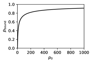
Figure 1: The lower bound of success probability of quantum spatial search for $p=p_{0}\frac{\log(n)}{n}$ for almost all graph from Erdős-Rényi graph model. The exact formula is $p_{\mathrm{bound}}=W_{0}\left(\frac{1-p_{0}}{\mathrm{e}p_{0}}\right)/W_{-1}\left(\frac{1-p_{0}}{\mathrm{e}p_{0}}\right)$. Note that $p_{\mathrm{bound}}\to 0$ as $p_{0}\to 1^{+}$, where connectivity threshold is achieved. Furthermore $p_{\mathrm{bound}}\to 1$ as $p_{0}\to\infty$

Theorem 3.

Suppose we chose a graph according to Erdős-Rényi $\mathcal{G}(n,p)$ model. For $p=\omega(\log(n)/n)$, by choosing $M_{G}=\frac{1}{np}L$ in Eq. (2), almost surely all vertices can be found with probability $1-o(1)$ in asymptotic $\pi\sqrt{n}/2$ time. For $p\sim p_{0}\log(n)/n$, by choosing $M_{G}=(1+r)\gamma L$ for some proper $r$, where $\gamma$ is defined as in Eq. (11), all vertices can be found in $\Theta(\sqrt{n})$ time with probability bounded from below by the constant in Eq. (12).

We leave determining proper $r$ and $t$ values as open question.

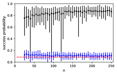
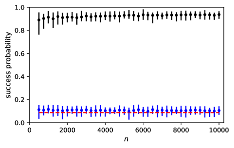
Figure 2: The figure presents probability bounds for quantum spatial search together with success probability derived from simulation. The red dashed line denotes the limit bound for succes probability. The blue error bars denote $\frac{1-c}{1+c}$ for $c=\max\{|\lambda_{2}|,|\lambda_{n}|\}$ for matrix from Eq. 11 for randomly chosen graph. Black error bars denote the actual success probability. Deviations correspond to the maximal and minimal obtained values. Graphs were chosen according to the $\mathcal{G}(n,2\frac{\log(n)}{n})$ model, $r$ were derived according to the Eq. 3 and we chose time $t=\frac{\pi\sqrt{n}}{2}$. 30 graphs were chosen for each size. One can see that the bound for randomly chosen graph oscillates around the limit value, nonetheless the true success probability is much higher than the bound.

Theorem 4.

Suppose we chose a graph according to Erdős-Rényi $\mathcal{G}(n,p)$ model with $p\leq(1-\varepsilon)\log(n)/n$, where $\varepsilon>0$. Then for both adjacency and Laplacian matrices there exist vertices which cannot be found in $o(n)$ time.

Conclusion and discussion.

In this work we prove that all vertices can be found optimally with common measurement time $(\pi\sqrt{n})/2$ for almost all Erdős-Rényi graphs for both adjacency and Laplacian matrices under conditions $p=\omega(\log^{8}(n)/n)$ and $p\geq(1+\varepsilon)\log(n)/n$ respectively. The proof is based on element-wise ergodicity of the eigenvector corresponding to the outlying eigenvalue of adjacency or Laplacian matrix. While under the mentioned constraint adjacency matrix almost surely achieves success probability $1-o(1)$, the same probability for Laplacian matrix in the $p\sim p_{0}\log(n)/n$ case for some $p_{0}>1$ can only be bounded from below by some positive constant. At the same time for $p<(1-\varepsilon)\log(n)/n$, the property does not hold anymore, since almost surely there exist isolated vertices which need $\Omega(n)$ time to be found.

While our derivation concerning the Laplacian matrix is nearlt complete, since only upper-bound for success probability is missing in the $p=\Theta(\log(n)/n)$ case, in our opinion it is possible to weaken the condition on $p$ for the adjacency matrix. The first key step would be showing that the largest eigenvalue $\lambda(\frac{1}{np}A)$ follows $\mathcal{N}(1,\frac{1}{n}\sqrt{2(1-p)/p)}$ distribution for $p\geq(1+\varepsilon)\log(n)/n$. Then, since element-wise convergence of principal vector requires $p=\omega(\log^{3}(n)/(n\log^{2}\log n))$, the result would be strengthened to the last mentioned constraint. The second step would be the generalization of the mentioned element-wise convergence theorem.

Further interesting generalization of the result would be the analysis of more general random graph models as well. While this proposition has already been stated [4], our results show that in order to prove security of the quantum spatial search, it would be desirable to analyze the limit behavior of the principal vector in the sense of $\|\cdot\|_{\infty}$ norm.

Acknowledgements Aleksandra Krawiec, Ryszard Kukulski and Zbigniew Puchała acknowledge the support from the National Science Centre, Poland under project number 2016/22/E/ST6/00062. Adam Glos was supported by the National Science Centre under project number DEC-2011/03/D/ST6/00413.

Appendix A Element-wise bound on principal eigenvector

Let $G_{n,p}$ be a random Erdős-Rényi graph, $\deg(v)$ be a degree of the vertex $v\in V$ and $A$ be its adjacency matrix with eigenvalues $\lambda_{1}\geq\lambda_{2}\geq\ldots\geq\lambda_{n}$. Let also $|\lambda_{i}\rangle$ be an eigenvector corresponding to the eigenvalue $\lambda_{i}$ and $|s\rangle=\frac{1}{\sqrt{n}}|\mathbf{1}\rangle=\frac{1}{\sqrt{n}}\sum_{i=1}^{n}|v\rangle$.

Proposition 5.

For the probability $p=\omega\left(\ln^{3}(n)/(n\log^{2}\log n)\right)$and some constant $c>0$ we have

$$\||\lambda_{1}\rangle-|s\rangle\|_{\infty}\leq c\frac{1}{\sqrt{n}}\frac{\ln^{3/2}(n)}{\sqrt{np}\ln(np)}$$ (13)

with probability $1-o(1)$.

Proof.

Using [20], we have

$$\|A-E(A)\|\leq\sqrt{8np\ln(n)},$$ (14)

$$|\lambda_{1}-np|\leq\sqrt{8np\ln(\sqrt{2}n)},$$ (15)

$$\underset{i\geq 2}{\max}|\lambda_{i}|\leq\sqrt{8np\ln(\sqrt{2}n)},$$ (16)

with probability $1-o(1)$. The first inequality was shown in the proof of Theorem 1 while the second and third inequalities come from Theorem 3 in [20]. Note $\deg(v)$ follows a binomial distribution. Using Lindenberg’s CLT and the fact that the convergence is uniform one can show that

$$\begin{split}P\left(|\deg(v)-np|\leq 2\sqrt{\ln(n)np(1-p)}\right)&\approx P\left(|\mathcal{X}|\leq 2\sqrt{\ln(n)}\right)\\ &\geq 1-\frac{1}{\sqrt{2\pi\ln(n)}n^{2}},\end{split}$$ (17)

where $\mathcal{X}$ is a random variable with standard normal distribution. Let $A=\lambda_{1}|\lambda_{1}\rangle\langle\lambda_{1}|+\sum_{i\geq 2}\lambda_{i}|\lambda_{i}\rangle\langle\lambda_{i}|$ and $|s\rangle=\alpha|\lambda_{1}\rangle+\beta|\lambda_{1}^{\perp}\rangle$. Assume that $|\lambda_{1}\rangle,|\lambda_{1}^{\perp}\rangle,|\lambda_{i}\rangle$ are normed vectors and $|\lambda_{1}^{\perp}\rangle=\sum_{i\geq 2}\gamma_{i}|\lambda_{i}\rangle$. By the Perron-Frobenius Theorem we can choose a vector $|\lambda_{1}\rangle$ such that $\langle{v}|{\lambda_{1}}\rangle\geq 0$ and hence obtain $\langle{s}|{\lambda_{1}}\rangle=\alpha>0$. Thus

$$\begin{split}&\left(A-E(A)\right)|\lambda_{1}\rangle\\ &=\left(\lambda_{1}|\lambda_{1}\rangle\langle\lambda_{1}|+\sum_{i\geq 2}\lambda_{i}|\lambda_{i}\rangle\langle\lambda_{i}|-np|s\rangle\langle s|\right)|\lambda_{1}\rangle\\ &=(\lambda_{1}-np\alpha^{2})|\lambda_{1}\rangle-np\alpha\beta|\lambda_{1}^{\perp}\rangle.\end{split}$$ (18)

With probability $1-o(1)$, using Eq. (14) we have

$$\begin{split}(\lambda_{1}-np\alpha^{2})^{2}+(np)^{2}\alpha^{2}\beta^{2}&=\|\left(A-E(A)\right)|\lambda_{1}\rangle\|^{2}\\ &\leq 8np\ln(n)\end{split}$$ (19)

and thus since $\beta^{2}=1-\alpha^{2}$, then

$$\alpha^{2}np(np-2\lambda_{1})+\lambda_{1}^{2}\leq 8np\ln(n).$$ (20)

Eventually, we receive

$$\begin{split}1\geq\alpha\geq\alpha^{2}&\geq\frac{\lambda_{1}^{2}-8np\ln(n)}{2\lambda_{1}np-(np)^{2}}\\ &\geq 1-\frac{4}{2+\sqrt{\frac{np}{8\ln(\sqrt{2}n)}}}\\ &\geq 1-\frac{16}{\sqrt{\frac{np}{\ln(n)}}},\end{split}$$ (21)

where the fourth inequality comes from Eq. (15). We know that $|\deg(v)-np|\leq 2\sqrt{n\ln(n)p(1-p)}$ with probability greater than $1-\frac{1}{n^{2}}$. Thus, with probability $1-\frac{1}{n}$ the above is true for all $v\in V$ simultaneously. Now, since $\deg(v)=\langle v|A|\mathbf{1}\rangle$, we have

$$\begin{split}\frac{np-2\sqrt{n\ln(n)p(1-p)}}{\lambda_{1}}&\leq\frac{1}{\lambda_{1}}\langle v|\texttt{}A|\mathbf{1}\rangle\\ &\leq\frac{np+2\sqrt{n\ln(n)p(1-p)}}{\lambda_{1}}\end{split}$$ (22)

The lower bound can be estimated as

$$\begin{split}\frac{np-2\sqrt{n\ln(n)p(1-p)}}{\lambda_{1}}&\overset{(\ref{eq:zal2})}{\geq}\frac{1-2\sqrt{\ln(n)\frac{1-p}{np}}}{1+\sqrt{8\frac{\ln(\sqrt{2}n)}{np}}}\\ &\geq\frac{1-2\sqrt{\frac{\ln(n)}{np}}}{1+4\sqrt{\frac{\ln(n)}{np}}}\eqqcolon d\end{split}$$ (23)

and similarly the upper bound

$$\frac{np+2\sqrt{n\ln(n)p(1-p)}}{\lambda_{1}}\leq\frac{1+2\sqrt{\frac{\ln(n)}{np}}}{1-4\sqrt{\frac{\ln(n)}{np}}}\eqqcolon u.$$ (24)

Consequently

$$\frac{d}{\sqrt{n}}\leq\frac{1}{\lambda_{1}}\langle v|A|s\rangle\leq\frac{u}{\sqrt{n}}$$ (25)

for all $v\in V$. Let $l=c\frac{\ln(n)}{\ln(\sqrt{\frac{np}{\ln(n)}}/4)}$, where $c=c(n,p)\in[1,2)$ is chosen to satisfy $l=\left\lceil\frac{\ln(n)}{\ln(\sqrt{\frac{np}{\ln(n)}}/4)}\right\rceil$. Hence

$$\frac{d^{l}}{\sqrt{n}}\leq\langle v|\left(\frac{A}{\lambda}\right)^{l}|s\rangle\leq\frac{u^{l}}{\sqrt{n}}$$ (26)

for all $v\in V$. On the other hand

$$\begin{split}\left(\frac{1}{\lambda_{1}}A\right)^{l}\left(\alpha|\lambda_{1}\rangle+\beta|\lambda_{1}^{\perp}\rangle\right)&=\left(|\lambda_{1}\rangle\langle\lambda_{1}|+\sum_{i\geq 2}\left(\frac{\lambda_{i}}{\lambda_{1}}\right)^{l}|\lambda_{i}\rangle\langle\lambda_{i}|\right)\left(\alpha|\lambda_{1}\rangle+\beta|\lambda_{1}^{\perp}\rangle\right)\\ &=\alpha|\lambda_{1}\rangle+\beta\sum_{i\geq 2}\left(\frac{\lambda_{i}}{\lambda_{1}}\right)^{l}\gamma_{i}|\lambda_{i}\rangle.\end{split}$$ (27)

Using Eq. (14,15) we are able to estimate $\frac{\lambda_{i}}{\lambda_{1}}$ by

$$\begin{split}\frac{\lambda_{i}}{\lambda_{1}}&\leq\frac{\sqrt{8np\ln(\sqrt{2}n)}}{np-\sqrt{8np\ln(\sqrt{2}n)}}\\ &=\frac{1}{\sqrt{\frac{np}{8\ln(\sqrt{2}n)}}-1}\leq\frac{4}{\sqrt{\frac{np}{\ln(n)}}}.\end{split}$$ (28)

Thus

$$\begin{split}\left\|\beta\sum_{i\geq 2}\left(\frac{\lambda_{i}}{\lambda_{1}}\right)^{l}\gamma_{i}|\lambda_{i}\rangle\right\|_{\infty}&\leq|\beta|\left\|\sum_{i\geq 2}\left(\frac{\lambda_{i}}{\lambda_{1}}\right)^{l}\gamma_{i}|\lambda_{i}\rangle\right\|_{2}\\ &\leq|\beta|\sqrt{\sum_{i\geq 2}\gamma_{i}^{2}\left(\frac{4}{\sqrt{\frac{np}{\ln(n)}}}\right)^{2l}}\\ &=\frac{|\beta|}{\left(\frac{\sqrt{\frac{np}{\ln(n)}}}{4}\right)^{l}}=\frac{|\beta|}{n^{c}}\\ &\leq\frac{4}{\left(\frac{np}{\ln(n)}\right)^{1/4}n},\end{split}$$ (29)

where the last inequality comes from Eq. (21) and $\|\cdot\|_{2}$ denotes the Euclidean norm. By Eq. (25,27) we get

$$\frac{d^{l}}{\sqrt{n}}\leq\alpha\langle{v}|{\lambda_{1}}\rangle+\langle v|\left(\beta\sum_{i\geq 2}\left(\frac{\lambda_{i}}{\lambda_{1}}\right)^{l}\gamma_{i}|\lambda_{i}\rangle\right)\leq\frac{u^{l}}{\sqrt{n}},$$ (30)

for all $v\in V$ and using Eq. (21,29) we eventually obtain

$$\frac{\frac{d^{l}}{\sqrt{n}}-\frac{4}{\left(\frac{np}{\ln(n)}\right)^{1/4}n}}{1}\leq\langle{v}|{\lambda_{1}}\rangle\leq\frac{\frac{u^{l}}{\sqrt{n}}+\frac{4}{\left(\frac{np}{\ln(n)}\right)^{1/4}n}}{1-\frac{16}{\sqrt{\frac{np}{\ln(n)}}}}$$ (31)

for all $v\in V$. In order to finish the proof it is necessary to show that

$$(1-d^{l})+\frac{4}{\left(\frac{np}{\ln(n)}\right)^{1/4}\sqrt{n}}=O\left(\frac{\ln^{3/2}(n)}{\sqrt{np}\ln(np)}\right)$$ (32)

and

$$(u^{l}-1)+\frac{4}{\left(\frac{np}{\ln(n)}\right)^{1/4}\sqrt{n}}=O\left(\frac{\ln^{3/2}(n)}{\sqrt{np}\ln(np)}\right).$$ (33)

We need to estimate how quickly $d^{l}$ converges to $1$. Using the fact that $d\rightarrow 1$, it is enough to observe that

$$(1-d)l=O\left(\frac{\ln^{3/2}(n)}{\sqrt{np}\ln\left(\sqrt{\frac{np}{\ln(n)}}/4\right)}\right),$$ (34)

and thus

$$1-d^{l}\approx 1-e^{(d-1)l}=O\left(\frac{\ln^{3/2}(n)}{\sqrt{np}\ln(np)}\right).$$ (35)

The second term of LHS of Eq. (32) converges to $0$ more rapidly than the bound, so it completes the proof for the lower bound. The same thing for the upper bound can be shown analogously. ∎

Appendix B Distribution of the largest eigenvalue of adjacency matrix

Theorem 6.2 from [19] considers the distribution of the largest eigenvalue of rescaled adjacency matrix $\tilde{A}=A/\sqrt{(1-p)pn}$. They show that as long as $p>\frac{1}{n}$, then

$$\mathbb{E}\lambda_{1}(\tilde{A})=\sqrt{\frac{np}{1-p}}+\sqrt{\frac{1-p}{np}}+o(1).$$ (36)

Furthermore, under another condition $p=\omega(\log^{8}(n)/n)$ we have

$$\sqrt{\frac{n}{2}}\left(\lambda_{1}(\tilde{A})-\mathbb{E}\lambda_{1}(\tilde{A})\right)\to\mathcal{N}(0,1)$$ (37)

in a distribution. This allows us to derive the distribution of the largest eigenvalue of the $\frac{1}{np}A$ matrix

$$\begin{split}\lambda_{1}\left(\frac{1}{np}A\right)&=\sqrt{\frac{1-p}{np}}\lambda_{1}(\tilde{A})\\ \ &=\frac{\sqrt{2(1-p)}}{n\sqrt{p}}\left(\sqrt{\frac{n}{2}}\left(\lambda_{1}(\tilde{A})-\mathbb{E}\lambda_{1}(\tilde{A})\right)+\sqrt{\frac{n}{2}}\mathbb{E}\lambda_{1}(\tilde{A})\right)\\ &=\frac{\sqrt{2(1-p)}}{n\sqrt{p}}\mathcal{X}+1+\frac{1-p}{np}+\sqrt{\frac{1-p}{np}}o(1)\end{split}$$ (38)

where $\mathcal{X}\to\mathcal{N}(0,1)$. Hence we have that $\lambda_{1}(\frac{1}{np}A)\sim\mathcal{N}(1,\frac{1}{n}\sqrt{\frac{2(1-p)}{p}})$. Note, that under the condition $p=\omega(\log^{8}(n)/n)$, the standard deviation tends to 0. This means that the largest eigenvalue actually tends to the Dirac distribution $\delta_{x=1}$.

This gives as a bound for $\lambda_{1}(\frac{1}{np}A)$. Note that

$$\mathbb{P}(|\lambda_{1}(A/(np))-1|\leq\delta)=1-\operatorname{erfc}\left(\frac{n\sqrt{p}\delta}{2\sqrt{1-p}}\right).$$ (39)

The probability tends to 1 as long as the argument tends to $\infty$. In order to achieve this, we need to assume $n\sqrt{p}\delta\to\infty$ as $n\to\infty$. This can be done by choosing $\delta=o(\frac{1}{n\sqrt{p}})$. Eventually, we have asymptotically almost surely

$$\left|\lambda_{1}\left(\frac{1}{np}A\right)-1\right|=o\left(\frac{1}{n\sqrt{p}}\right).$$ (40)

Note that for $p=o(1)$ the bound is better than the one used in [4].

Appendix C Laplacian matrix spectrum

Algebraic connectivity satisfies $\mu_{n-1}=np+O(\sqrt{np\log n})$ for $p=\omega(\log(n)/n)$. Similarly we conclude from results of Bryc et al. [22], that $\mu_{1}\sim np$.

Theorem 6.

Let $L_{n}$ be a Laplacian matrix of random Erdős-Rényi graph $\mathcal{G}(n,p)$, where $p=\omega(\frac{\log n}{n})$. Then $\mu_{1}=\mu(L)\sim np$.

Proof.

By Theorem 1.5 from [22], if $\tilde{L}$ is a symmetric matrix whose off-diagonal elements have two-points distribution with mean 0 and variance $p(1-p)$ and $\tilde{L}_{ii}=\sum_{j\neq i}\tilde{L}_{ij}$. Then

$$\lim_{n\to\infty}\frac{\mu(\tilde{L})}{\sqrt{2np(1-p)\log n}}=1.$$ (41)

Note that in the following version $p$ may depend on $n$. Hence, we can extend the Corollary 1.6 from the same paper.

Let $L_{n}=\tilde{L}_{n}+Y_{n}$, where $Y_{n}$ is a deterministic matrix with $-p$ on off-diagonal and $(n-1)p$ on diagonal. Note that $Y_{n}$ is an expectation of a random Erdős-Rényi Laplacian matrix. $Y_{n}$ has a single 0 eigenvalue and all of the others take the form $np$. By this we have $\mu(Y_{n})=\|Y_{n}\|=np$. Then we have

$$\left|\frac{\|L_{n}\|}{np}-\frac{\|Y_{n}\|}{np}\right|\leq\frac{\|L_{n}-Y_{n}\|}{np}=\frac{\|\tilde{L}_{n}\|}{np}\to 0$$ (42)

where the limit comes from the Eq. (41), assuming $p=\omega(\log n/n)$. Finally $\frac{\mu(L_{n})}{np}\to 1$. ∎

Appendix D The largest eigenvalue of Laplacian matrix near the connectivity treshold

Suppose $G$ is a random graph chosen according to $\mathcal{G}(n,p_{0}\frac{\log(n)}{n})$ distribution, for $p_{0}>1$ being a constant. It can be shown, that

$$\delta\sim(1-p_{0})\left(W_{-1}\left(\frac{1-p_{0}}{\mathrm{e}p_{0}}\right)\right)^{-1}\log(n)$$ (43)

and

$$\Delta\sim(1-p_{0})\left(W_{0}\left(\frac{1-p_{0}}{\mathrm{e}p_{0}}\right)\right)^{-1}\log(n),$$ (44)

see [21], Exercise III.4. Here $\delta$ and $\Delta$ denote respectively minimal and maximal degree of the graph. In [23] authors have shown that providing

$$|\delta-cnp|=O(\sqrt{np})$$ (45)

we have

$$|\mu_{n-1}-cnp|=O(\sqrt{np}),$$ (46)

where $\mu_{n-1}$ is the second smallest eigenvalue of the Laplacian matrix. In fact, similar behavior can be stated for the largest eigenvalue, i.e. if

$$|\Delta-cnp|=o(np)$$ (47)

we have

$$|\mu_{1}-cnp|=o(np).$$ (48)

While we plan to prove the statement above, it is possible that the RHS can be reduced to $O(\sqrt{np})$ by following the proof in [23]. Nonetheless, we are satisfied with the mentioned result. The proof is very similar to the proof of Lemma 3.4 in [23]. Furthermore, note, that the theorem holds for $p_{0}>0$.

Theorem 7.

Suppose there exists a $p_{0}>0$ so that $np\geq p_{0}\log(n)$ and $\Delta\sim cnp$ almost surely. Then almost surely $\mu_{1}\sim cnp$.

Proof.

Note, that since the eigenvector corresponding to 0 eigenvalue is the equal superposition, we have

$$\begin{split}\mu_{1}&=\max_{\{|\phi\rangle\bot|s\rangle:\langle{\phi}|{\phi}\rangle=1\}}\langle\phi|L|\phi\rangle\\ &=\max_{\{|\phi\rangle\bot|s\rangle:\langle{\phi}|{\phi}\rangle=1\}}(\langle\phi|D|\phi\rangle-\langle\phi|A|\phi\rangle).\end{split}$$ (49)

Note that

$$\begin{split}\mu_{1}&\leq\max_{\{|\phi\rangle\bot|s\rangle:\langle{\phi}|{\phi}\rangle=1\}}\langle\phi|D|\phi\rangle+\max_{\{|\phi\rangle\bot|s\rangle:\langle{\phi}|{\phi}\rangle=1\}}|\langle\phi|A|\phi\rangle)|\\ &\leq\Delta+C\sqrt{np}\end{split}$$ (50)

by Theorem 2.5 from [24]. Similarly one can show $\mu_{1}\geq\Delta$, which can be done by taking maximum over canonical vectors. After combining those bounds and $\Delta\sim cnp$, we obtain the result. ∎

References

- [1] A. M. Childs and J. Goldstone, “Spatial search by quantum walk,” Physical Review A, vol. 70, no. 2, p. 022314, 2004.
- [2] A. M. Childs, R. Cleve, E. Deotto, E. Farhi, S. Gutmann, and D. A. Spielman, “Exponential algorithmic speedup by a quantum walk,” in Proceedings of the thirty-fifth annual ACM symposium on Theory of computing, pp. 59–68, ACM, 2003.
- [3] A. Ambainis, “Quantum walks and their algorithmic applications,” International Journal of Quantum Information, vol. 1, no. 04, pp. 507–518, 2003.
- [4] S. Chakraborty, L. Novo, A. Ambainis, and Y. Omar, “Spatial search by quantum walk is optimal for almost all graphs,” Physical review letters, vol. 116, no. 10, p. 100501, 2016.
- [5] G. D. Paparo and M. Martin-Delgado, “Google in a quantum network,” Scientific reports, vol. 2, p. 444, 2012.
- [6] G. D. Paparo, M. Müller, F. Comellas, and M. A. Martin-Delgado, “Quantum Google in a complex network,” Scientific reports, vol. 3, 2013.
- [7] E. Sánchez-Burillo, J. Duch, J. Gómez-Gardenes, and D. Zueco, “Quantum navigation and ranking in complex networks,” Scientific reports, vol. 2, 2012.
- [8] O. Mülken, V. Pernice, and A. Blumen, “Quantum transport on small-world networks: A continuous-time quantum walk approach,” Physical Review E, vol. 76, no. 5, p. 051125, 2007.
- [9] O. Mülken and A. Blumen, “Continuous-time quantum walks: Models for coherent transport on complex networks,” Physics Reports, vol. 502, no. 2, pp. 37–87, 2011.
- [10] J. Roland and N. J. Cerf, “Noise resistance of adiabatic quantum computation using random matrix theory,” Physical Review A, vol. 71, no. 3, p. 032330, 2005.
- [11] S. Chakraborty, L. Novo, S. Di Giorgio, and Y. Omar, “Optimal quantum spatial search on random temporal networks,” Phys. Rev. Lett., vol. 119, p. 220503, 2017.
- [12] A. Tulsi, “Success criteria for quantum search on graphs,” arXiv preprint arXiv:1605.05013, 2016.
- [13] P. Philipp, L. Tarrataca, and S. Boettcher, “Continuous-time quantum search on balanced trees,” Physical Review A, vol. 93, no. 3, p. 032305, 2016.
- [14] T. G. Wong, “Spatial search by continuous-time quantum walk with multiple marked vertices,” Quantum Information Processing, vol. 15, no. 4, pp. 1411–1443, 2016.
- [15] T. G. Wong, L. Tarrataca, and N. Nahimov, “Laplacian versus adjacency matrix in quantum walk search,” Quantum Information Processing, vol. 15, no. 10, pp. 4029–4048, 2016.
- [16] D. E. Knuth, “Big omicron and big omega and big theta,” ACM Sigact News, vol. 8, no. 2, pp. 18–24, 1976.
- [17] P. Erdős and A. Rényi, “On the evolution of random graphs,” Publ. Math. Inst. Hung. Acad. Sci, vol. 5, no. 1, pp. 17–60, 1960.
- [18] P. Mitra, “Entrywise bounds for eigenvectors of random graphs,” The electronic journal of combinatorics, vol. 16, no. 1, p. R131, 2009.
- [19] L. Erdős, A. Knowles, H.-T. Yau, J. Yin, and others, “Spectral statistics of Erdős-Rényi graphs I: local semicircle law,” The Annals of Probability, vol. 41, no. 3B, pp. 2279–2375, 2013.
- [20] F. Chung and M. Radcliffe, “On the spectra of general random graphs,” The electronic journal of combinatorics, vol. 18, no. 1, p. P215, 2011.
- [21] B. Bollobás, “Random graphs. 2001,” Cambridge Stud. Adv. Math, 2001.
- [22] W. Bryc, A. Dembo, and T. Jiang, “Spectral measure of large random Hankel, Markov and Toeplitz matrices,” The Annals of Probability, pp. 1–38, 2006.
- [23] T. Kolokolnikov, B. Osting, and J. Von Brecht, “Algebraic connectivity of Erdős-Rényi graphs near the connectivity threshold,” Manuscript in preparation, 2014.
- [24] U. Feige and E. Ofek, “Spectral techniques applied to sparse random graphs,” Random Structures & Algorithms, vol. 27, no. 2, pp. 251–275, 2005.