Lyapunov-Based Stabilization and Control of the Stochastic Schrödinger Equation

Abstract

This paper presents a detailed Lyapunov-based theory to control and stabilize continuously-measured quantum systems, which are driven by Stochastic Schrödinger Equation (SSE). Initially, equivalent classes of states of a quantum system are defined and their properties are presented. With the help of equivalence classes of states, we are able to consider global phase invariance of quantum states in our mathematical analysis. As the second mathematical modelling tool, the conventional Itö formula is further extended to non-differentiable complex functions. Based on this extended Itö formula, a detailed stochastic stability theory is developed to stabilize the SSE. Main results of this proposed theory are sufficient conditions for stochastic stability and asymptotic stochastic stability of the SSE. Based on the main results, a solid mathematical framework is provided for controlling and analyzing quantum system under continuous measurement, which is the first step towards implementing weak continuous feedback control for quantum computing purposes.

1 Introduction

Building quantum computers have been one of the most notable research efforts in the past decades. The idea of quantum computing started with the famous proposal of Richard Feynman of Simulating physics with computers Feynman (1982). Although the original idea of Feynman was to simulate a quantum mechanical system with another quantum system, it turned out that exploiting purely quantum mechanical features is significantly applicable to other engineering demands Dowling and Milburn (2003). These engineering applications mainly include secure communication Renner (2008), fast and efficient data processing DiVincenzo (1995) in addition to simulating nano-scale systems.

Computing with devices at nano scales demands building, manipulating, and efficiently measuring such tiny devices, which is a challenging task. There must be a worthwhile payoff for performing engineering tasks at this level despite these complications. The key element, which makes quantum systems unique, is quantum coherence. This phenomenon lives at nano scales and disappears as the system approaches the classical limit. This many-fold complexity of systems at nano scales makes it exponentially hard to simulate them with classical computers and classical bits. That is why it is almost impossible to simulate and analytically calculate the energy levels of simple molecular structures with classical computers. On the other hand, it has been shown that some classical hard problems can be solved in polynomial time on a hypothetical quantum computer Shor (1999).

The lifesaver property of quantum coherence dies out (decoherence happens) in two main situations, namely uncontrolled interaction of the quantum system with environment, which is undesirable and almost unavoidable Viola et al. (1999) and when the system is measured, which is unavoidable since at some point, the results must be acquired from the system. Therefore, measurement alters the state of the system and inevitably destroys its quantum features Busch (2009). This seems to be a turning point in quantum computing. Fortunately, the introduction of weak measurement and weak values Aharonov et al. (1988); Jozsa (2007); Brun (2002) turned the page. By weakly measuring a quantum system, we can maintain the quantum coherence at the cost of acquiring noisier information about the system Jacobs (2014). Recently, implementing weak continuous measurement of qubits has attracted theoreticians and experimentalists in the area of quantum computing Muhonen et al. (2018); Pfender et al. (2019); Ran et al. (2019); Shojaee et al. (2018); Gross et al. (2018); Vijay et al. (2012). Noisy information about the system is not the only complication induced by implementing weak continuous measurement; dynamics of these quantum systems are also governed by Stochastic Schrödinger Equation (SSE) Wiseman (1996), which takes into account the back-action of weak continuous measurement in the form of additional stochastic terms to the ordinary Schrödinger Equation Breuer and Petruccione (2002); Jacobs and Steck (2006); Wiseman (1994). Controlling and analyzing the stochastic quantum system governed by SSE, requires more consideration and more sophisticated mathematical tools, provided by stochastic and nonlinear control theory Sontag (2013); Khalil (1996); Sastry (2013); Khasminskii (2011); Kushner (1967). In this paper, the aim is to provide a solid mathematical framework (through control theory) to analyze, stabilize, and manipulate quantum systems in the presence of weak continuous measurement, in order to ease the way of implementing this framework for quantum computing purposes.

Lyapunov theory was initially used for quantum systems analysis in Grivopoulos and Bamieh (2003). Following this idea, in early 2000’s, many researchers started to use Lyapunov theory for controlling and stabilization of Schrödinger equation Kuang and Cong (2008); Mirrahimi et al. (2005); Wang and Schirmer (2010). Lyapunov theory has been among the important theories to analyze quantum systems in recent years Wang et al. (2014); Kuang et al. (2018); Ghaeminezhad and Cong (2018); Cardona et al. (2020); Liu et al. (2019); Jie et al. (2018). For instance, Lyapunov theory has been used to stabilize two-level quantum systems Cardona et al. (2018); Qamar and Cong (2019). Despite its importance and experimental applications, stabilization of an open quantum system under continuous measurement has not received the attraction it deserves.

In this paper, we use stochastic Lyapunov theory stability analysis of continuously -measured quantum systems. In quantum physics, global phase gauge invariance induces some difficulties to control purposes. This is due to the fact that some states may be distinguishable from a mathematical viewpoint, but represent the same quantum state. In order to overcome this difficulty, equivalent classes of quantum states are defined and some of their useful properties are studied. The conventional Itö formalism is not capable of evaluating the stochastic increment for the proposed Lyapunov function. Hence, initially, the Itö formalism is extended to non-analytic complex functions. Then, based on the extended Itö formula, the stochastic increment of the Lyapunov function can be evaluated. The Lyapunov function considered in this paper, which is defined based on the well-known Hilbert-Schmidt distance Prugovecki (1982), is highly adaptable to the proposed extended Itö formula. The main results of this paper are two stochastic stability theorems. The first theorem provides the conditions on the desired final state, the Hamiltonian, and the observable that guarantee stochastic stability of the quantum system. In the second part, it is shown that some additional conditions on the control Hamiltonians lead to stochastic asymptotic stability of the quantum system. In this paper, it is assumed that the control system is Equivalent State Controllable (ESC), i.e. it is always possible to find a set of control signals to make the transition between any two arbitrary equivalent classes of states in a finite time interval d’Alessandro (2007). The conditions proposed for asymptotic stochastic stability are reasonably more strict than Equivalent State Controllability (ESC) conditions, since in addition to steering the system, these conditions also guarantee stochastic stability.

This paper consists of the following sections: In section 2, some preliminary background is presented and the problem is formulated. This section mainly introduces continuously-measured quantum systems and their dynamic behaviour. Also, in the problem formulation subsection, some assumptions are defined to be used in the next sections. In section 3, the Lyapunov candidate is defined and the Itö formula is extended to suite non-analytic complex functions. In section 4, main results on the stochastic stability of quantum systems are developed. First, two definitions are presented, afterward, the main results are presented within some lemmas and theorems. In section 5, the proposed theorem is validated via an illustrative example of a qubit system, and section 6 provides concluding remarks.

2 Preliminaries and Problem Formulation

2.1 Quantum Dynamical Systems

According to the postulates of quantum mechanics, our state of knowledge about a finite dimensional ($n$-level) quantum system can be described by a normalized vector $\left|\psi\right\rangle\in{S^{2n-1}}$, where ${S^{2n-1}}=\mathcal{H}$ is the unit hypersphere $\mathbb{C}^{n}$, together with the Euclidean inner product $\left\langle{.}\mathrel{\left|{\vphantom{..}}\right.\kern-1.2pt}{.}\right\rangle$. The time evolution of a closed quantum system is governed by the Schrödinger wave equation:

$$\begin{array}[]{l}\frac{d}{{dt}}\left|{\psi(t)}\right\rangle=\frac{{-i}}{\hbar}H\left|{\psi(t)}\right\rangle,\left|{\psi(0)}\right\rangle=\left|{{\psi_{0}}}\right\rangle\end{array}$$ (1)

where $H$($iH\in su(n)$) is a bounded (and equivalently compact) self-adjoint operator, called system Hamiltonian.

The relative phase invariance in quantum mechanics has led to some difficulties in modeling quantum control systems. By this invariance, all the states $e^{i\varrho}\left|\psi\right\rangle$ with $\varrho\in\mathbb{R}$ correspond to the same quantum state. In order to overcome this difficulty, the following definition is adapted:

D 1.

$\left[{\left|{{\psi}}\right\rangle}\right]\doteq\left\{{{e^{i\varrho}}\left|{{\psi}}\right\rangle\left|{\varrho\in\mathbb{R}}\right.}\right\}$ is the equivalence class of $\left|{{\psi}}\right\rangle$ and two different quantum states $\left|{{\psi_{1}}}\right\rangle$ and $\left|{{\psi_{2}}}\right\rangle$ are said to be equivalent if $\left|{{\psi_{1}}}\right\rangle\in\left[{\left|{{\psi_{2}}}\right\rangle}\right]$.

The quotient space corresponding to this partitioning is infinite dimensional even if we consider a finite dimensional quantum system.

The following lemma will be useful in the rest of this article:

Lemma 1.

Consider two non-equivalent quantum states, i.e. $\left|{{\psi_{1}}}\right\rangle\notin\left[{\left|{{\psi_{2}}}\right\rangle}\right]$, there exists $\epsilon>0$ and a self adjoint operator $H^{\prime}$(${\left\|{H^{\prime}}\right\|_{HS}}=1$, $H^{\prime}\neq I$) such that:

$$\left|{{\psi_{1}}}\right\rangle={e^{i\varepsilon H^{\prime}}}{\left|{{\psi_{2}}}\right\rangle}$$ (2)

Also, neither of $\left|{{\psi_{1}}}\right\rangle$ and $\left|{{\psi_{2}}}\right\rangle$ is an eigenket of $H^{\prime}$.

Sketch of the proof.

The transitivity property of $SU(n)$ as a Lie transformation group and its Homeomorphism to $su(n)$ by the exponential map provide the main idea for the proof. Also, both of the following conditions:

1. $H^{\prime}=I$

2. Any one of $\left|{{\psi_{1}}}\right\rangle$ or $\left|{{\psi_{2}}}\right\rangle$ being an eigenket for $H^{\prime}$

contradicts the non-equivalence property. ∎

2.2 Continuously measured quantum systems

By the early postulates of quantum mechanics, the measurement process, projects the system into the eigenspace corresponding to the resulting eigenket of the observable. This viewpoint is known as projective measurement or also, strong Von Neumann measurement. By this postulate, the pre-measure quantum state is completely missed. Developing Positive Operator Valued Measure (POVM) led to a more general model for quantum measurement, known as weak measurement Brun (2002); Aharonov et al. (1988). By weak measurement, the pre-measure state, does not necessarily collapse to the eigenstates of the observable but deviates from its initial state. This deviation depends on the strength of the measurement and the distribution spread of the Gaussian measurement. Moreover, the obtained information is unsharp. This phenomena obeys the Busch’s theorem: “no information without disturbance”Busch (2009).

A continuously measured quantum system is the one being continuously weakly measured. Let us denote the measurement observable by $X$, which is neccesarily self adjoint. In Jacobs and Steck (2006); Jacobs (2014), a Gaussian approach to weak measurement is followed. In this approach, the deviation of the premeasure state depends on the measurement strength and the energy shifts between the eigenkets of $X$ weighted by the projection of pre-measure state into the eigenbasis generated by $X$. In the case of continuous measurement, this approach leads to the following stochastic dynamic behaviour, known as Stochastic Schrödinger Equation:

$$d\left|\psi\right\rangle=\left({(-k{{(X-\left\langle X\right\rangle)}^{2}})dt+\sqrt{2k}(X-\left\langle X\right\rangle)dW}\right)\left|\psi\right\rangle,$$ (3)

where $k$ is the strength of the measurement, $dW$ is the standard Wiener process, and $\left\langle X\right\rangle$ is the expected value of the observable $X$. Also, it is shown that the contribution of the free evolution term in (1) added together with (3), (i.e. the complete evolution) is given by:

$$\begin{gathered}d\left|\psi\right\rangle=\left({(\frac{{-i}}{\hbar}H-k{{(X-\left\langle X\right\rangle)}^{2}})dt+\sqrt{2k}(X-\left\langle X\right\rangle)dW}\right)\left|\psi\right\rangle.\\ \left|{\psi(0)}\right\rangle=\left|{{\psi_{0}}}\right\rangle{\text{; a}}{\text{.s}}.\\ \end{gathered}$$ (4)

This stochastic unitary evolution is a more general form of strong measurement. One may deduce from (4) that in the case of great measurement strength, the quantum system is projected to the eigenkets of $X$ in a short time. For convenience let us use the following notation:

$$\hat{f}(\left|\psi\right\rangle)\doteq\left({\frac{{-i}}{\hbar}H-k{{(X-\left\langle X\right\rangle)}^{2}}}\right)\left|\psi\right\rangle,\hat{g}(\left|\psi\right\rangle)\doteq\left({\sqrt{2k}(X-\left\langle X\right\rangle)}\right)\left|\psi\right\rangle,$$ (5)

where $\hat{f}$ and $\hat{g}$ are the drift and diffusion terms, respectively. Obviously, $\hat{f}$ and $\hat{g}$ admit the Lipschitz continuity and growth condition, thus, the existence and uniqueness of the strong solution of (4) and the quantum trajectories are guaranteed.

2.3 Problem formulation

Dynamic behavior of an open quantum system with Hamiltonian $H$, which is continuously measured by $X$, was studied in section 2.2. In order to address the control issue, consider the following assumptions:

A 1.

Consider the set of control signals $U\doteq\left\{{{u_{k}}(t)\left|{k=1,...,m;{u_{k}}\in{L^{2}}(\mathbb{R})}\right.}\right\}$. Each of the Lebesgue measurable control signals ${u_{k}}(t)$ is associated with a compact control Hamiltonian $H_{k}$ ($iH_{k}\in su(n)$) as its coefficient and they appear in the Hamiltonian in an affine manner:

$${H}(U)={{H}_{0}}+\sum\limits_{k}{{u_{k}}(t)}{{H}_{k}}.$$ (6)

The free evolution Hamiltonian $H(0)=H_{0}$ describes the system in the absence of a control field.

The previous assumption is not restrictive. In practice, the manipulation signals usually appear in an affine form (e.g. the effect of an interacting magnetic field on a spin system). Although the observable $X$ participates in the manipulation, in this article, we just address the role of control signals in the stabilization procedure. In the rest of this article, our aim is to analyze the stability properties of the quantum trajectories, driven by the nonlinear stochastic differential equation (4). The quantum trajectories start from the initial state $\left|{{\psi_{0}}}\right\rangle$ almost surely and the aim is to manipulate them to the equivalent class of the desired final state $\left[{\left|{{\psi_{f}}}\right\rangle}\right]$. For convenience, the point spectrum (the compactness of $H_{0}$ and the separability of the underlying Hilbert space imply that the continuous and residual spectrum of $H_{0}$ are empty) of $H_{0}$ is denoted by $\sigma({H_{0}})\doteq\left\{{{\lambda_{i}}}\right\}$ and the eigenspace conjugate to $\lambda_{i}$ is denoted by $\sigma_{\lambda_{i}}({H_{0}})$.

A 2.

The desired final state ${\left|{{\psi_{f}}}\right\rangle}$ (and also $\left[{\left|{{\psi_{f}}}\right\rangle}\right]$) is an eigenstate of $H_{0}$ with eigenvalue ${\lambda_{Hf}}$( i.e.,$\left[{\left|{{\psi_{f}}}\right\rangle}\right]\in\sigma_{\lambda_{Hf}}({H_{0}})$) and the corresponding eigenspace is degenerate.

A 3.

The desired final state ${\left|{{\psi_{f}}}\right\rangle}$ is not an eigenstate of $H_{k}$ for at least one $k$ i.e., $\exists k;\left[{\left|{{\psi_{f}}}\right\rangle}\right]\notin\bigcup\limits_{j}{{\sigma_{{\lambda_{j}}}}({H_{k}})}$.

In the upcoming sections, it will be shown that the control Hamiltonians containing ${\left|{{\psi_{f}}}\right\rangle}$ as their eigenstate do not contribute to the manipulation process.

A 4.

The desired final state ${\left|{{\psi_{f}}}\right\rangle}$ is an eigenstate of $X$ with eigenvalue ${\lambda_{Xf}}$. i.e., $\left[{\left|{{\psi_{f}}}\right\rangle}\right]\in\sigma_{\lambda_{Xf}}({X})$.

A 5.

The control Hamiltonian set $\left\{{{H_{k}}}\right\}$ has at least $n-1$ elements, any of which does not have ${\left|{{\psi_{f}}}\right\rangle}$ as its eigenket, and the Hamiltonians $\left\{{{H_{0}},{H_{1}},...,{H_{n-1}}}\right\}$ constitute an $n$-element linearly independent set.

In the rest of this article, each of these assumptions will help to derive the desired results. In the next section, the stabilization process and the stochastic boundedness analysis are studied for the formulated problem by the use of extended Lyapunov theory.

3 Extended stochastic Lyapunov theory

The process of designing control signals $U$ to achieve the desired goals, is inspired by stochastic Lyapunov theory. This theory is highly dependent on the Itö formula, which gives the increment of the Lyapunov function according to a continuous Feller (and thus, strong Markov) stochastic process. In the problem of manipulating a quantum system, we are faced with a difficulty in using the conventional Itö formula. In this section, it is shown that the proposed Lyapunov function is not differentiable when we employ the complex numbers as the field for our Hilbert space.

3.1 Lyapunov function

In this article, a Lyapunov function is employed, which is based on maximizing the transition probability to the desired final state:

$$V(\left|\psi\right\rangle)=\frac{1}{2}\left({1-{{\left|{\left\langle{{{\psi_{f}}}}\mathrel{\left|{\vphantom{{{\psi_{f}}}\psi}}\right.\kern-1.2pt}{\psi}\right\rangle}\right|}^{2}}}\right)$$ (7)

This Lyapunov function (which is obviously positive) is inspired by the Hilbert-Schmidt norm of an operator. In what follows, the advantages of this Lyapunov candidate will become clear. First, the mathematical properties of (7) is discussed within some lemmas:

Lemma 2.

Consider the Lyapunov function in (7), the following statements are equivalent:

1. $V(\left|\psi\right\rangle)=0$

2. $\left|\psi\right\rangle=\left[{\left|{\psi{}_{f}}\right\rangle}\right]$

Proof.

(b)$\rightarrow$(a) is obvious. For (a)$\rightarrow$(b), the sufficient condition for (a) is ${\left|{\left\langle{{{\psi_{f}}}}\mathrel{\left|{\vphantom{{{\psi_{f}}}\psi}}\right.\kern-1.2pt}{\psi}\right\rangle}\right|^{2}}=1$. Using the fact that both $\left|\psi\right\rangle$ and $\left|\psi_{f}\right\rangle$ are normalized, by Cauchy$-$Bunyakovsky$-$Schwarz inequality, the necessary and sufficient condition is $\left|\psi\right\rangle=c\left|\psi_{f}\right\rangle$ with $|c|=1$, which means (b) by D1. ∎

This lemma plays an important role in guaranteeing asymptotic stability properties in the rest of this article. By this lemma, vanishing Lyapunov function exclusively describes the convergence of the quantum trajectories to the equivalence class of the desired final state. The following lemma will play an important role in asymptotic stability of the quantum trajectories in upcoming sections.

Lemma 3.

Consider the Lyapunov function in (7), suppose that $\left|{{\psi}}\right\rangle\notin\left[{\left|{{\psi_{f}}}\right\rangle}\right]$ and $0<R\leqslant\left\|{\left|\psi\right\rangle-[\left|{{\psi_{f}}}\right\rangle]}\right\|<2$ ($\left|\psi\right\rangle$ is not in an open $R$-neighbourhood of the set $[\left|{{\psi_{f}}}\right\rangle]$), then $V(\left|\psi\right\rangle)$ is bounded away from zero i.e., there exists $\nu(R)>0$ such that $\nu(R)\leqslant V(\left|\psi\right\rangle)$.

Proof.

The assumption reads ${R^{2}}\leqslant\left\langle{{\psi-{e^{-i\varepsilon}}{\psi_{f}}}}\mathrel{\left|{\vphantom{{\psi-{e^{i\varepsilon}}{\psi_{f}}}{\psi-{e^{i\varepsilon}}{\psi_{f}}}}}\right.\kern-1.2pt}{{\psi-{e^{i\varepsilon}}{\psi_{f}}}}\right\rangle$ for all real $\epsilon$, which leads to:

$${R^{2}}\leqslant 2-2\operatorname{Re}({e^{-i\varepsilon}}\left\langle{{{\psi_{f}}}}\mathrel{\left|{\vphantom{{{\psi_{f}}}\psi}}\right.\kern-1.2pt}{\psi}\right\rangle).$$

Take $\left\langle{{{\psi_{f}}}}\mathrel{\left|{\vphantom{{{\psi_{f}}}\psi}}\right.\kern-1.2pt}{\psi}\right\rangle=r{e^{i\theta}}$, where $r$ and $\theta$ depend on $\left|\psi\right\rangle$, and choose $\epsilon=-\theta$. Thus, for all admissible $\left|\psi\right\rangle$, one may write:

$$r\leqslant 1-\frac{{{R^{2}}}}{2}.$$

The above inequality reads:

$$\mathop{\sup}\limits_{{\text{admissible }}\left|\psi\right\rangle}\left|{\left\langle{{{\psi_{f}}}}\mathrel{\left|{\vphantom{{{\psi_{f}}}\psi}}\right.\kern-1.2pt}{\psi}\right\rangle}\right|\leqslant 1-\frac{{{R^{2}}}}{2}$$

Also, it can be shown that the supremum takes the RHS value on the boundary of admissible closed set of $\left|\psi\right\rangle$. Thus, one may define $\nu(R)\doteq{R^{2}}-\frac{{{R^{4}}}}{4}$. ∎

3.2 Extended Itö formula

The common well-known Itö formula, gives the increment of a scalar function, of a strong Markov process driven by Itö form of stochastic differential equations. It is necessary that the function be twice-differentiable. When we treat a complex-field Hilbert space, our definition on the differentiablility changes (The complex function must necessarily admit Cauchy-Riemann condition). The sufficient condition for extending the common Itö formalism to the complex case is the holomorphism of the complex function, which is highly restrictive. The proposed Lyapunov function (7), is neither holomorphic, nor even differentiable in its domain (of course employing a holomorphic Lyapunov function is very restrictive and does not necessarily satisfy the mentioned conditions). In this section, the common Itö formula is extended to undifferentiable complex functions. In order to proceed, the following definitions, which are induced from Gâteaux differentiation, are presented:

D 2.

Consider the complex (not necessarily differentiable) function $V(\left|\psi\right\rangle):{S^{2n-1}}\mapsto\mathbb{R}$.

1. If there exists a functional ${\nabla}V:{\mathbb{C}^{n}}\mapsto\mathbb{C}^{n}$, independent of $\left|\partial\psi\right\rangle$ such that the following limit exists for any fixed $\left|\partial\psi\right\rangle\in{\mathbb{C}^{n}}$:

   $$\mathop{\lim}\limits_{h\downarrow 0}\frac{{V(\left|\psi\right\rangle+h\left|{\partial\psi}\right\rangle)-V(\left|\psi\right\rangle)-h\left({{\nabla}V(\left|\psi\right\rangle)}\right)\left|{\partial\psi}\right\rangle}}{h}=0,$$ (8)

   then ${\nabla}V(\left|\psi\right\rangle)$ is called the directional gradient in the direction $\left|\partial\psi\right\rangle$.

2. Assuming that ${\nabla}V(\left|\psi\right\rangle)$ exists, if there exists an operator ${\nabla^{2}}V(\left|\psi\right\rangle):{\mathbb{C}^{n}}\mapsto\mathbb{C}^{n\times n}$, independent of $\left|\partial\psi\right\rangle$ such that the following limit exists:

   $$\mathop{\lim}\limits_{h\downarrow 0}\frac{{V(\left|\psi\right\rangle+h\left|{\partial\psi}\right\rangle)-V(\left|\psi\right\rangle)-h\left({{\nabla}V(\left|\psi\right\rangle)}\right)\left|{\partial\psi}\right\rangle-\frac{{{h^{2}}}}{2}\left\langle{\partial\psi}\right|\left({{\nabla^{2}}V(\left|\psi\right\rangle)}\right)\left|{\partial\psi}\right\rangle}}{{{h^{2}}}}=0$$ (9)

   then, ${\nabla^{2}}V(\left|\psi\right\rangle)$ is called the second order directional gradient in the direction $\left|\partial\psi\right\rangle$.

The previous definitions of the directional gradients, pave the way for analyzing the functional properties of (7). The directional gradients for (7) are evaluated as:

$$\begin{gathered}{\nabla}V(\left|\psi\right\rangle)=-\operatorname{Re}(\left\langle{\psi}\mathrel{\left|{\vphantom{\psi{{\psi_{f}}}}}\right.\kern-1.2pt}{{{\psi_{f}}}}\right\rangle\left\langle{{\psi_{f}}}\right|)\\ {\nabla^{2}}V(\left|\psi\right\rangle)=-\left|{{\psi_{f}}}\right\rangle\left\langle{{\psi_{f}}}\right|\\ \end{gathered}$$ (10)

where $\operatorname{Re}(\left\langle.\right|)\doteq\frac{1}{2}\left({\left\langle{.}\mathrel{\left|{\vphantom{.\psi}}\right.\kern-1.2pt}{\psi}\right\rangle+\left\langle{\psi}\mathrel{\left|{\vphantom{\psi.}}\right.\kern-1.2pt}{.}\right\rangle}\right)$ which acts on $\left|\psi\right\rangle$. In the next proposition, it is shown that first and second order gradients will help us to exactly evaluate the perturbed Lyapunov function.

Proposition 1.

For the proposed Lyapunov function (7), define ${d_{\partial\left|\psi\right\rangle}}V(\left|\psi\right\rangle)\doteq{V(\left|\psi\right\rangle+\left|{\partial\psi}\right\rangle)-V(\left|\psi\right\rangle)}$ for sufficiently small $\left|{\partial\psi}\right\rangle$, then with the directional gardients in (10), the following equality holds:

$${d_{\left|{\partial\psi}\right\rangle}}V(\left|\psi\right\rangle)=\left({{\nabla}V(\left|\psi\right\rangle)}\right)\left|{\partial\psi}\right\rangle+\frac{1}{2}\left\langle{\partial\psi}\right|\left({{\nabla^{2}}V(\left|\psi\right\rangle)}\right)\left|{\partial\psi}\right\rangle$$ (11)

Proof.

$$\begin{gathered}{d_{\left|{\partial\psi}\right\rangle}}V(\left|\psi\right\rangle)=\frac{{-1}}{2}\left({\left\langle{{{\psi_{f}}}}\mathrel{\left|{\vphantom{{{\psi_{f}}}{\psi+\partial\psi}}}\right.\kern-1.2pt}{{\psi+\partial\psi}}\right\rangle\left\langle{{\psi+\partial\psi}}\mathrel{\left|{\vphantom{{\psi+\partial\psi}{{\psi_{f}}}}}\right.\kern-1.2pt}{{{\psi_{f}}}}\right\rangle-\left\langle{{{\psi_{f}}}}\mathrel{\left|{\vphantom{{{\psi_{f}}}\psi}}\right.\kern-1.2pt}{\psi}\right\rangle\left\langle{\psi}\mathrel{\left|{\vphantom{\psi{{\psi_{f}}}}}\right.\kern-1.2pt}{{{\psi_{f}}}}\right\rangle}\right)\hfill\\ {\text{ }}=\frac{{-1}}{2}\left({\left\langle{{{\psi_{f}}}}\mathrel{\left|{\vphantom{{{\psi_{f}}}\psi}}\right.\kern-1.2pt}{\psi}\right\rangle\left\langle{{\partial\psi}}\mathrel{\left|{\vphantom{{\partial\psi}{{\psi_{f}}}}}\right.\kern-1.2pt}{{{\psi_{f}}}}\right\rangle+\left\langle{{{\psi_{f}}}}\mathrel{\left|{\vphantom{{{\psi_{f}}}{\partial\psi}}}\right.\kern-1.2pt}{{\partial\psi}}\right\rangle\left\langle{\psi}\mathrel{\left|{\vphantom{\psi{{\psi_{f}}}}}\right.\kern-1.2pt}{{{\psi_{f}}}}\right\rangle+\left\langle{{{\psi_{f}}}}\mathrel{\left|{\vphantom{{{\psi_{f}}}{\partial\psi}}}\right.\kern-1.2pt}{{\partial\psi}}\right\rangle\left\langle{{\partial\psi}}\mathrel{\left|{\vphantom{{\partial\psi}{{\psi_{f}}}}}\right.\kern-1.2pt}{{{\psi_{f}}}}\right\rangle}\right)\hfill\\ {\text{ }}=\left({\nabla V(\left|\psi\right\rangle)}\right)\left|{\partial\psi}\right\rangle+\frac{1}{2}\langle\partial\psi|\left({{\nabla^{2}}V(\left|\psi\right\rangle)}\right)\left|{\partial\psi}\right\rangle.\hfill\\ \end{gathered}$$

∎

This proposition presents the directional counterpart of the Taylor series for an undifferentiable real-valued complex function (This is why the directional gradients were defined. Although this Lyapunov function is not analytic, a Taylor-like serie is presented). Also this proposition shows why this Lyapunov candidate suits the problem of manipulating the SSE. The value of perturbed Lyapunov function is exactly evaluated by two perturbation steps.

Based on the presented definitions, in the next theorem, the extended version of the Itö formula for undifferentiable complex functions of a strong Markov process is presented. This extended version of the Itö formula is the starting point to use the stochastic Lyapunov theory.

Theorem 1.

Let $V:{S^{2n-1}}\mapsto\mathbb{R}$ be a real function with well-defined directional gradients defined in D2. Also, assume that (11) holds and $\left|\psi\right\rangle$ be an adapted stochastic process driven by the following Itö drift-diffusion stochastic differential equation:

$$d\left|\psi\right\rangle=f(\left|\psi\right\rangle)dt+g(\left|\psi\right\rangle)dW.$$ (12)

Then, the following equality holds for the stochastic increment of $V$:

$${d_{d\left|\psi\right\rangle}}V(\left|\psi\right\rangle) =\left({{\nabla}V(\left|\psi\right\rangle)f(\left|\psi\right\rangle)+\frac{1}{2}{{\left({g(\left|\psi\right\rangle)}\right)}^{\dagger}}{\nabla^{2}}V(\left|\psi\right\rangle)\left({g(\left|\psi\right\rangle)}\right)}\right)dt$$ (13)

$$+\left({{\nabla}V(\left|\psi\right\rangle)g(\left|\psi\right\rangle)}\right)dW.$$

Proof.

Substituting (12) into (11) in place of ${\left|{\partial\psi}\right\rangle}$ gives:

$$\begin{gathered}{d_{d\left|\psi\right\rangle}}V(\left|\psi\right\rangle)={\nabla}V(\left|\psi\right\rangle)f(\left|\psi\right\rangle)dt+{\nabla}V(\left|\psi\right\rangle)g(\left|\psi\right\rangle)dW\\ {\text{ }}+\frac{1}{2}\left(\begin{gathered}{\left({f(\left|\psi\right\rangle)}\right)^{\dagger}}{\nabla^{2}}V(\left|\psi\right\rangle)\left({f(\left|\psi\right\rangle)}\right){(dt)^{2}}\hfill\\ +{\left({g(\left|\psi\right\rangle)}\right)^{\dagger}}{\nabla^{2}}V(\left|\psi\right\rangle)\left({g(\left|\psi\right\rangle)}\right){(dW)^{2}}\hfill\\ +{\left({g(\left|\psi\right\rangle)}\right)^{\dagger}}{\nabla^{2}}V(\left|\psi\right\rangle)\left({f(\left|\psi\right\rangle)}\right)(dtdW)\hfill\\ +{\left({f(\left|\psi\right\rangle)}\right)^{\dagger}}{\nabla^{2}}V(\left|\psi\right\rangle)\left({g(\left|\psi\right\rangle)}\right)(dtdW)\hfill\\ \end{gathered}\right).\\ \end{gathered}$$ (14)

Keeping terms up to $(dW)^{2}$ and integrating in the sense of Itö, gives:

$$\begin{gathered}V(\left|{\psi(t)}\right\rangle)=\int_{0}^{t}{{\nabla}V(\left|\psi\right\rangle)f(\left|\psi\right\rangle)dt}+\int_{0}^{t}{{\nabla}V(\left|\psi\right\rangle)g(\left|\psi\right\rangle)dW}\\ +\frac{1}{2}\int_{0}^{t}{{{\left({g(\left|\psi\right\rangle)}\right)}^{\dagger}}{\nabla^{2}}V(\left|\psi\right\rangle)\left({g(\left|\psi\right\rangle)}\right){{(dW)}^{2}}}\\ \end{gathered}$$ (15)

Using the Itö multiplication rule for the third integral gives Chen et al. (1995):

$$\begin{gathered}V(\left|{\psi(t)}\right\rangle)=\int_{0}^{t}{\left({{\nabla}V(\left|\psi\right\rangle)f(\left|\psi\right\rangle)+\frac{1}{2}{{\left({g(\left|\psi\right\rangle)}\right)}^{\dagger}}{\nabla^{2}}V(\left|\psi\right\rangle)\left({g(\left|\psi\right\rangle)}\right)}\right)dt}\\ +\int_{0}^{t}{{\nabla}V(\left|\psi\right\rangle)g(\left|\psi\right\rangle)dW}.\\ \end{gathered}$$ (16)

Therefore, the Itö form of stochastic differential equation for $V(\left|\psi\right\rangle)$ is:

$$\begin{gathered}{d_{d\left|\psi\right\rangle}}V(\left|\psi\right\rangle)=\left({{\nabla}V(\left|\psi\right\rangle)f(\left|\psi\right\rangle)+\frac{1}{2}{{\left({g(\left|\psi\right\rangle)}\right)}^{\dagger}}{\nabla^{2}}V(\left|\psi\right\rangle)\left({g(\left|\psi\right\rangle)}\right)}\right)dt\\ +\left({{\nabla}V(\left|\psi\right\rangle)g(\left|\psi\right\rangle)}\right)dW.\\ \end{gathered}$$ (17)

∎

In the rest of this paper, the coefficient of $dt$ will be denoted by ${L_{d\left|\psi\right\rangle}}V(\left|\psi\right\rangle)$ or ${L}V(\left|\psi\right\rangle)$.

Remark 1.

The previous theorem presents the stochastic increment of $V(\left|\psi\right\rangle)$. This increment is evaluated by keeping terms up to $O(dt)$, which is reasonable since $dt\rightarrow 0$. Also, for the complex functions with directional gradients not satisfying (11), one can derive (13) in the second order approximation, which is valid as $dt\rightarrow 0$.

For the Lyapunov function (7), with directional gradients in (10), one may deduce that the stochastic increment of $V(\left|\psi\right\rangle)$ regarding the SSE defined by (4) and driven by the control field in (6) has the following form:

$$\begin{gathered}{d_{d\left|\psi\right\rangle}}V(\left|\psi\right\rangle)=\left(\begin{gathered}\frac{{-1}}{\hbar}\operatorname{Im}\left({\left\langle{\psi}\mathrel{\left|{\vphantom{\psi{{\psi_{f}}}}}\right.\kern-1.2pt}{{{\psi_{f}}}}\right\rangle\left\langle{{\psi_{f}}}\right|H(U)\left|\psi\right\rangle}\right)\\ +k\operatorname{Re}\left({\left\langle{\psi}\mathrel{\left|{\vphantom{\psi{{\psi_{f}}}}}\right.\kern-1.2pt}{{{\psi_{f}}}}\right\rangle\left\langle{{\psi_{f}}}\right|{{\left({X-\left\langle X\right\rangle}\right)}^{2}}\left|\psi\right\rangle}\right)\hfill\\ -k{\left|{\left\langle{{\psi_{f}}}\right|\left({X-\left\langle X\right\rangle}\right)\left|\psi\right\rangle}\right|^{2}}\hfill\\ \end{gathered}\right)dt\\ -\sqrt{2k}\operatorname{Re}\left({\left\langle{\psi}\mathrel{\left|{\vphantom{\psi{{\psi_{f}}}}}\right.\kern-1.2pt}{{{\psi_{f}}}}\right\rangle\left\langle{{\psi_{f}}}\right|\left({X-\left\langle X\right\rangle}\right)\left|\psi\right\rangle}\right)dW.\\ \end{gathered}$$ (18)

Based on the proposed mathematical background, in the following sections, main results on the stability of quantum trajectories are presented.

4 Main results on the stability of the SSE

4.1 Definitions

The stochastic properties, studied in this article are constructed on the complete probability space $(\Omega,\Xi,\operatorname{P})$, where $\Omega$ is the sample space, $\Xi$ is the $\sigma$-algebra generated by $\Omega$ and $\operatorname{P}$ is a probability measure defined on $\Xi$. Let us consider a quantum stochastic process, which is the solution of SSE (4), by $\left|{{\psi}(\omega,t)}\right\rangle:\left({\Omega\times T,\Xi\otimes{{\rm B}(T)}}\right)\mapsto\left({{\mathcal{H}},{\rm B}({\mathcal{H}})}\right)$ and a quantum trajectory (a sample path of $\left|{{\psi}(\omega,t)}\right\rangle$) started from $\left|\psi_{0}\right\rangle$ at $t=0$ by $\left|{{\psi^{\left|{{\psi_{0}}}\right\rangle}}(t)}\right\rangle:T\mapsto\mathcal{H}$, where $T\doteq\left[{0,\infty}\right)$ is the time index and $\rm B(.)$ denotes the Borel $\sigma$-algebra generated by the corresponding set.

Lemma 2 provides that support of $V$ ($\operatorname{supp}(V)=\left\{{\left|\psi\right\rangle\notin\left[{\left|{{\psi_{f}}}\right\rangle}\right]}\right\}$), is compact in ${\mathbb{C}^{n}}$, thus ${L}V(\left|\psi\right\rangle)$ is the infinitesimal generator of $V(\left|\psi\right\rangle)$, i.e.,

$$LV(\left|{{\psi^{\left|{{\psi_{0}}}\right\rangle}}(t)}\right\rangle)=\mathop{\lim}\limits_{h\downarrow 0}\frac{{\operatorname{E}\left[{V\left({\left|{\psi(\omega,t+h)}\right\rangle}\right)}\right]-V\left({\left|{{\psi^{\left|{{\psi_{0}}}\right\rangle}}(t)}\right\rangle}\right)}}{h}.$$ (19)

Based on the previous sections, we propose two definitions on the stability of quantum trajectories.

D 3.

The quantum stochastic process $\left|{\psi(\omega,t)}\right\rangle\equiv\left[{\left|{{\psi_{f}}}\right\rangle}\right]$ driven by (4) is said to be:

1. stochastically stable if for any $0<\epsilon$:

   $$\mathop{\lim}\limits_{\left\|{\left|{\partial\psi}\right\rangle}\right\|\to 0}\operatorname{P}\left\{{\mathop{\sup}\limits_{0\leqslant t}\left\|{\left|{{\psi^{\left|{{\psi_{f}}}\right\rangle+\left|{\partial\psi}\right\rangle}}(t)}\right\rangle-\left[{\left|{{\psi_{f}}}\right\rangle}\right]}\right\|\geqslant\varepsilon}\right\}=0$$ (20)

2. stochastically asymptotically stable if it is stochastically stable and also:

   $$\mathop{\lim}\limits_{\left\|{\left|{\partial\psi}\right\rangle}\right\|\to 0}P\left\{{\mathop{\sup}\limits_{0\leqslant t}\left\|{\left|{{\psi^{\left|{{\psi_{f}}}\right\rangle+\left|{\partial\psi}\right\rangle}}(t)}\right\rangle-\left[{\left|{{\psi_{f}}}\right\rangle}\right]}\right\|=0}\right\}=1.$$ (21)

The previous definitions presented two notions of stability for the considered quantum trajectories. A stable quantum trajectory remains in a neighbourhood of the equivalence class of the desired final state almost surely as the initial value approaches that equivalence class. The second notion guarantees that the quantum trajectory does not escape the equivalence class almost surely.

4.2 Stochastic stability of SSE

In order to study the stability of quantum trajectories, the conditions $\hat{f}(\left[{\left|{{\psi_{f}}}\right\rangle}\right])=\hat{g}(\left[{\left|{{\psi_{f}}}\right\rangle}\right])={\mathbf{0}}$ must necessarily hold. These conditions are satisfied if A2 and A4 are satisfied in addition to the condition that control signals $U$ vanish at $\left[{\left|{{\psi_{f}}}\right\rangle}\right]$. Thus A2 and A4 are the basic necessary assumptions in the rest of this section. Also one may deduce that according to A2 and A4, the infinitesimal generator ${L}V(\left|\psi\right\rangle)$ in (18) takes the following form:

$$LV(\left|\psi\right\rangle)=-\frac{1}{\hbar}\sum\limits_{k=1}^{n}{{u_{k}}(t)}\operatorname{Im}\left({\left\langle{\psi}\mathrel{\left|{\vphantom{\psi{{\psi_{f}}}}}\right.\kern-1.2pt}{{{\psi_{f}}}}\right\rangle\left\langle{{\psi_{f}}}\right|{H_{k}}\left|\psi\right\rangle}\right).$$ (22)

Now the necessity of A3 is more obvious. In the absence of A3, the SSE (4) would be uncontrollable since all the coefficients of control signals in (22) would vanish everywhere in ${S^{2n-1}}$. In the rest of this paper, the following control signals will be used:

$${u_{k}}(t)={\alpha_{k}}\operatorname{Im}\left({{e^{i\measuredangle\left\langle{\psi}\mathrel{\left|{\vphantom{\psi{{\psi_{f}}}}}\right.\kern-1.2pt}{{{\psi_{f}}}}\right\rangle}}\left\langle{{\psi_{f}}}\right|\left.{{H_{k}}}\right|\left.\psi\right\rangle}\right),$$ (23)

where ${\alpha_{k}}\in{\mathbb{R}^{+}}$. This control signal has also been used for stabilizing the deterministic Schrödinger equation Shuang and KUANG (2007). Using the proposed control signals yields:

$$LV(\left|\psi\right\rangle)=-\frac{1}{\hbar}\sum\limits_{k=1}^{n}{{\alpha_{k}}}\left|{\left\langle{\psi}\mathrel{\left|{\vphantom{\psi{{\psi_{f}}}}}\right.\kern-1.2pt}{{{\psi_{f}}}}\right\rangle}\right|{\left({\operatorname{Im}\left({{e^{i\measuredangle\left\langle{\psi}\mathrel{\left|{\vphantom{\psi{{\psi_{f}}}}}\right.\kern-1.2pt}{{{\psi_{f}}}}\right\rangle}}\left\langle{{\psi_{f}}}\right|{H_{k}}\left|\psi\right\rangle}\right)}\right)^{2}}\leqslant 0.$$ (24)

Now, the following lemma can be stated:

Lemma 4.

Consider the Lyapunov function (7) where the quantum dynamic is driven by (4) with control signals (23). Then the process $V(\left|\psi\right\rangle)$ is a supermartingale. Also, $\mathop{\lim}\limits_{t\to\infty}\operatorname{E}[V(\left|\psi\right\rangle)]$ exists and is equal to $\operatorname{E}[V(\mathop{\lim}\limits_{t\to\infty}\left|{{\psi^{\left|{{\psi_{f}}}\right\rangle}}(\omega,t)}\right\rangle)]$.

Proof.

The fact that SSE (4) is a unitary evolution induces that $\operatorname{P}\left\{{{\tau_{m}}<\infty}\right\}=1$, where $\tau_{m}$ is the first exit time from ${Q_{m}}\doteq\left\{{\left|\psi\right\rangle\left|{V(\left|\psi\right\rangle)<m}\right.}\right\}$, i.e., ${\tau_{m}}\doteq\inf\left\{{t\left|{\left|{{\psi^{\left|{{\psi_{0}}}\right\rangle}}(t)}\right\rangle\notin{Q_{m}}}\right.}\right\}$ with $\left|{{\psi_{0}}}\right\rangle\in{Q_{m}}$ almost surely and $1<m$. Thus, $\tau\wedge t=t$ ($\tau\wedge t$ denotes $\min(\tau,t)$) almost surely for all $t$. Also, take ${\Gamma_{t}}$ the family of $\sigma$-algebras of sets of $\Xi$ generated by the Wiener processes $dW$up to time $t$. Now using Dynkins formula gives Kushner (1967):

$$\operatorname{E}[V\left({\left|{\psi\left({\omega,\left({t+h}\right)\wedge{\tau_{m}}}\right)}\right\rangle}\right)\left|{{\Gamma_{t}}}\right.]=V\left({\left|{\psi(\omega,t)}\right\rangle}\right)+\int_{t}^{(t+h)\wedge{\tau_{m}}}{LV\left({\left|{\psi(\omega,u)}\right\rangle}\right)}du.$$ (25)

Thus,

$$\operatorname{E}[V\left({\left|{\psi\left({\omega,t+h}\right)}\right\rangle}\right)\left|{{\Gamma_{t}}}\right.]\leqslant V\left({\left|{\psi(\omega,t)}\right\rangle}\right)$$ (26)

which results the supermartingale property. The fact that $V(\left|\psi\right\rangle)$ is a non-negative supermartingale gives that $\mathop{\lim}\limits_{t\to\infty}\operatorname{E}[V(\left|\psi\right\rangle)]$ exists and is equal to
$\operatorname{E}[V(\mathop{\lim}\limits_{t\to\infty}\left|{{\psi^{\left|{{\psi_{f}}}\right\rangle}}(\omega,t)}\right\rangle)]$ Doob (1953). ∎

Now take $0<R<2$ and define ${N_{R}}\doteq\left\{{\left|\psi\right\rangle\left|{\left\|{\left|\psi\right\rangle-\left|{{\psi_{f}}}\right\rangle}\right\|}\right.\leqslant R}\right\}$. Assume that $\left|{{\psi_{0}}}\right\rangle=\left|{{\psi_{f}}}\right\rangle+\left|{\partial\psi}\right\rangle\in{N_{R}}$ almost surely. If ${\tau_{{N_{R}}}}\doteq\inf\left\{{t\left|{\left|{{\psi^{\left|{{\psi_{0}}}\right\rangle}}\left(t\right)}\right\rangle\notin}\right.{N_{R}}}\right\}$ be the first exit time from $N_{R}$, by Lemma 4 one may deduce:

$$\operatorname{E}[V\left({\left|{\psi\left({\omega,{\tau_{{N_{R}}}}\wedge t}\right)}\right\rangle}\right)\left|{{\Gamma_{t}}}\right.]\leqslant V\left({\left|{{\psi_{0}}}\right\rangle}\right)$$ (27)

which expresses that the stopped process $V\left({\left|{\psi\left({\omega,{\tau_{{N_{R}}}}\wedge t}\right)}\right\rangle}\right)$ is also a supermartingale. Based on these derivations, the following theorem is presented, which plays an important role in stabilization procedure and shows the stochastic stability of ${\left|{{\psi_{f}}}\right\rangle}$ .

Theorem 2.

Consider the SSE (4) with assumptions discussed in section 2.2. Assume that A1 to A4 hold. With control signals (23), the quantum stochastic process $\left|{\psi(\omega,t)}\right\rangle\equiv\left[{\left|{{\psi_{f}}}\right\rangle}\right]$ is stochastically stable.

Proof.

Assume that $\left|{{\psi_{0}}}\right\rangle=\left|{{\psi_{f}}}\right\rangle+\left|{\partial\psi}\right\rangle\in{N_{R}}$ for some $0<R<2$ . By Lemma 4 and (27), one writes:

$$\operatorname{E}[\mathop{\sup}\limits_{0<t}V\left({\left|{{\psi^{\left|{{\psi_{0}}}\right\rangle}}\left({{\tau_{{N_{R}}}}\wedge t}\right)}\right\rangle}\right)]\leqslant V\left({\left|{{\psi_{0}}}\right\rangle}\right).$$ (28)

Defining $y(w)\doteq\mathop{\sup}\limits_{0<t}\left\|{\left|{{\psi^{\left|{{\psi_{0}}}\right\rangle}}\left({{\tau_{{N_{R}}}}\wedge t}\right)}\right\rangle-\left[{\left|{{\psi_{f}}}\right\rangle}\right]}\right\|$ and $\Omega^{\prime}\doteq\left\{{\omega\left|{R\leqslant y(\omega)}\right.}\right\}$, (28) can be rewritten as:

$$\begin{gathered}V\left({\left|{{\psi_{0}}}\right\rangle}\right)\geqslant\int\limits_{\Omega}{\mathop{\sup}\limits_{0<t}V\left({\left|{{\psi^{\left|{{\psi_{0}}}\right\rangle}}\left({{\tau_{{N_{R}}}}\wedge t}\right)}\right\rangle}\right)d\operatorname{P}}(\omega)\hfill\\ \hskip 36.98866pt\geqslant\int\limits_{\Omega^{\prime}}{\mathop{\sup}\limits_{0<t}V\left({\left|{{\psi^{\left|{{\psi_{f}}}\right\rangle+\left|{\partial\psi}\right\rangle}}\left({{\tau_{{N_{R}}}}\wedge t}\right)}\right\rangle}\right)d\operatorname{P}}(\omega)\hfill\\ \hskip 36.98866pt\geqslant\left(\mathop{\inf}\limits_{\Omega^{\prime}}{\mathop{\sup}\limits_{0<t}V\left({\left|{{\psi^{\left|{{\psi_{f}}}\right\rangle+\left|{\partial\psi}\right\rangle}}\left({{\tau_{{N_{R}}}}\wedge t}\right)}\right\rangle}\right)}\right)\operatorname{P}\left\{{y>R}\right\}.\hfill\\ \end{gathered}$$ (29)

By Lemma 3 one may deduce:

$$\operatorname{P}\left\{{\mathop{\sup}\limits_{t}\left\|{\left|{{\psi^{\left|{{\psi_{f}}}\right\rangle+\left|{\partial\psi}\right\rangle}}\left(t\right)}\right\rangle-\left[{\left|{{\psi_{f}}}\right\rangle}\right]}\right\|>R}\right\}\leqslant\frac{{V\left({\left|{{\psi_{0}}}\right\rangle}\right)}}{{\nu(R)}}.$$ (30)

Now, Lemma 2 and the continuity of $V(\left|\psi\right\rangle)$ give:

$$\mathop{\lim}\limits_{\left\|{\left|{\partial\psi}\right\rangle}\right\|\to 0}\operatorname{P}\left\{{\mathop{\sup}\limits_{t}\left\|{\left|{{\psi^{\left|{{\psi_{f}}}\right\rangle+\left|{\partial\psi}\right\rangle}}\left(t\right)}\right\rangle-\left[{\left|{{\psi_{f}}}\right\rangle}\right]}\right\|>R}\right\}\leqslant\mathop{\lim}\limits_{\left\|{\left|{\partial\psi}\right\rangle}\right\|\to 0}\frac{{V\left({\left|{{\psi_{0}}}\right\rangle}\right)}}{{\nu(R)}}=0.$$ (31)

∎

Theorem 2 reveals that the desired final state ${\left|{{\psi_{f}}}\right\rangle}$ is stochastically stable and the trajectories remain in any prescribed neighbourhood of ${\left[{\left|{{\psi_{f}}}\right\rangle}\right]}$ with probability $1$. Also, $\left|{{\psi_{0}}}\right\rangle\in\left[{\left|{{\psi_{f}}}\right\rangle}\right]$ is a special case of this result. In the rest of this section, we will show that under some conditions on the control Hamiltonians in (6), the stochastic asymptotic stability can be achieved.

4.3 Stochastic Asymptotic stability of SSE

Theorem 2 represented a stability condition on the quantum trajectories based on (24). In this sense, the system would evolve until reaching its invariant set, which is itself a subset of $\left\{{\left[{\left|\psi\right\rangle}\right]\left|{LV(\left|\psi\right\rangle)=0}\right.}\right\}$. In order to characterize this set, let us denote the set of eigenvalues of control Hamiltonians by $\sigma({H})\doteq\bigcup\limits_{k}{\sigma({H_{k}})}$. Also, based on the Cartan decomposition of $su(n)$, one can always find a basis, in which $H_{0}$ is diagonal. Denote this basis by $\left\{{\left|1\right\rangle,\left|2\right\rangle,...,\left|n\right\rangle}\right\}$, where the bases are mutually orthogonal. Without loss of generality, assume that the eigenspace corresponding to ${\left|1\right\rangle}$ is degenerate and $\left|{{\psi_{f}}}\right\rangle=\left|1\right\rangle$. Now using (24), the following theorem can be stated:

Theorem 3.

Consider the state dynamics (4) and the Lyapunov function (7), also assume that A1 to A5 hold. The set of quantum states, in which $LV(\left|\psi\right\rangle)=0$, can be decomposed into the following two subsets (i.e. $\left\{{\left|\psi\right\rangle\left|{LV(\left|\psi\right\rangle)=0}\right.}\right\}=A\cup B$):

• $A={\left[{\left|{{\psi_{f}}}\right\rangle}\right]^{\bot}}$

• $B=\left\{{\left|\psi\right\rangle\left|{\forall k,\exists{\lambda_{k}}\in\mathbb{R}:\left\langle{{{\psi_{f}}}}\mathrel{\left|{\vphantom{{{\psi_{f}}}{{H_{k}}-{\lambda_{k}}I\left|\psi\right.}}}\right.\kern-1.2pt}{{{H_{k}}-{\lambda_{k}}I\left|\psi\right.}}\right\rangle=0}\right.}\right\}$
  Also, the following statements hold:

  1. In the case that the control Hamiltonians $\left\{H_{k}\right\}$ have no common eigenkets, $B$ includes at most one equivalence class of states for each choise of $\left\{{{\lambda_{k}}\in\mathbb{R},k=1,...,n-1}\right\}$.

  2. In the case that the control Hamiltonians $\left\{H_{k}\right\}$ have $s$ independent common eigenkets (each of them is an eigenket for at least $2$ of the Hamiltonians) then $B$ includes at most $1+s$ different equivalence classes of quantum states.

  3. $\left[{\left|{{\psi_{f}}}\right\rangle}\right]\in B$ for some choice of $\left\{{{\lambda_{k}}\in\mathbb{R}-\sigma({H})}\right\}$.

Before proceeding with the proof, let us present a lemma which will be used in the proof of this theorem.

Lemma 5.

Consider the control Hamiltonians in (6). Assume that A1 to A5 hold. Then, for each choice of $\left\{{{\lambda_{k}}\in\mathbb{R},k=1,...,n-1}\right\}$, the set
$\left\{{H_{1}}-\lambda_{1}I,{H_{2}}-\lambda_{2}I,...,{H_{n-1}}-\lambda_{n-1}I\right\}$ is linearly independent.

Proof.

Without loss of generality assume that $\lambda_{1}\neq 0$. By contradiction assume that

$$\left\{{H_{1}}-\lambda_{1}I,{H_{2}}-\lambda_{2}I,...,{H_{n-1}}-\lambda_{n-1}I\right\}$$

is linearly dependent. Thus for some nonzero set $\left\{c_{2},...,{c_{n-1}}\right\}$ one may find an scalar $\alpha$ such that:

$$\alpha({H_{1}}-{\lambda_{1}}I)=\sum\limits_{k=2}^{n-1}{{c_{k}}({H_{k}}-{\lambda_{k}}I)}\Rightarrow\alpha{H_{1}}=\sum\limits_{k=2}^{n-1}{\left({{c_{k}}{H_{k}}}\right)}-\sum\limits_{k=2}^{n-1}{\left({{c_{k}}{\lambda_{k}}}\right)}I+\alpha{\lambda_{1}}I.$$

By the fact that $i{H_{k}}\in su(n)$ (and thus they are traceless), one has the unique choice of $\alpha=\frac{{\sum\limits_{k=2}^{n-1}{\left({{c_{k}}{\lambda_{k}}}\right)}}}{{{\lambda_{1}}}}$. So one deduces that:

$$\alpha{H_{1}}=\sum\limits_{k=2}^{n-1}{\left({{c_{k}}{H_{k}}}\right)}$$ (32)

which contradicts the assumption A5 in both cases $\alpha=0$ and $\alpha\neq 0$. ∎

proof of Theorem 3.

Due to (24), the space perpendicular to ${\left[{\left|{{\psi_{f}}}\right\rangle}\right]^{\bot}}$ belongs to $\left\{{\left|\psi\right\rangle\left|{LV(\left|\psi\right\rangle)=0}\right.}\right\}$, which shows $A$. In this proof, first we neglect the unitarity of the quantum state, and after finding the un-normalized solution subspace, it will be intersected with the unit sphere. Assume that $\mathbb{R}$ is partitioned as $\mathbb{R}=\left({\mathbb{R}-\sigma({H_{k}})}\right)\cup\sigma({H_{k}})$. If ${\left|{{\psi_{0}}}\right\rangle}\notin{\left[{\left|{{\psi_{f}}}\right\rangle}\right]^{\bot}}$, (24) implies that we should search for the common solutions of ${\operatorname{Im}\left({{e^{i\measuredangle\left\langle{\psi}\mathrel{\left|{\vphantom{\psi{{\psi_{f}}}}}\right.\kern-1.2pt}{{{\psi_{f}}}}\right\rangle}}\left\langle{{\psi_{f}}}\right|{H_{k}}\left|\psi\right\rangle}\right)}=0$ for all $k$, but:

$$\operatorname{Im}\left({{e^{i\measuredangle\left\langle{{{\psi_{f}}}}\mathrel{\left|{\vphantom{{{\psi_{f}}}\psi}}\right.\kern-1.2pt}{\psi}\right\rangle}}\langle{\psi_{f}}|{H_{k}}\left|\psi\right\rangle}\right)=0\Leftrightarrow\langle{\psi_{f}}|{H_{k}}\left|\psi\right\rangle={\lambda_{k}}\left\langle{{{\psi_{f}}}}\mathrel{\left|{\vphantom{{{\psi_{f}}}\psi}}\right.\kern-1.2pt}{\psi}\right\rangle\Leftrightarrow\langle{\psi_{f}}|{H_{k}}-{\lambda_{k}}I\left|\psi\right\rangle=0$$ (33)

for real $\lambda_{k}$’s.
Let us first prove (B.i). Assume that ${{\lambda_{k}}\in\mathbb{R}-\sigma({H_{k}})}$ for all $k$. Thus, ${H_{k}}-{\lambda_{k}}I$ is non-singular. Hence, we may characterize the subspace, which the solutions of (33) belong to for each $k$ as:

$${S_{k}}(\lambda_{k})\doteq\operatorname{span}\left\{{{{\left({{H_{k}}-{\lambda_{k}}I}\right)}^{-1}}\left|2\right\rangle,...,{{\left({{H_{k}}-{\lambda_{k}}I}\right)}^{-1}}\left|n\right\rangle}\right\},$$ (34)

which is an $(n-1)-$dimensional subspace regarding to linear independence of $\left|i\right\rangle$’s. Thus, the solution of (33) must necessarily belong to the intersection of ${S_{k}}(\lambda_{k})$’s for each choice of $\left\{{{\lambda_{k}}\in\mathbb{R}-\sigma({H_{k}})}\right\}$:

$$\left|\psi\right\rangle\in{\bigcap\limits_{k}{{S_{k}}({\lambda_{k}})}}.$$ (35)

By A5 and Lemma 5, we may deduce that none of the subspaces ${S_{k}}(\lambda_{k})$ can exactly coincide. For further demonstrations, one may show that
$\sum\limits_{j=2}^{n}{\left\langle j\right|({H_{t}}-{\lambda_{t}}I){{({H_{u}}-{\lambda_{u}}I)}^{-1}}\left|1\right\rangle}\left|j\right\rangle$ belongs to ${S_{t}}(\lambda_{t})$ but not ${S_{u}}(\lambda_{u})$ for each pair of distinct $u$ and $t$ $\in\left\{1,2,...,n-1\right\}$. Also, for each distinct $s$, $u$, and $t$, $\sum\limits_{j=2}^{n}{\left\langle j\right|({H_{t}}-{\lambda_{t}}I){{({H_{u}}-{\lambda_{u}}I)}^{-1}}\left|1\right\rangle}\left|j\right\rangle$ and $\sum\limits_{j=2}^{n}{\left\langle j\right|({H_{s}}-{\lambda_{s}}I){{({H_{u}}-{\lambda_{u}}I)}^{-1}}\left|1\right\rangle}\left|j\right\rangle$ cannot be collinear (based on Lemma 5). The dimension of intersection of $n-1$ non-coincident $(n-1)-$dimensional subspaces is not more than $1$. Now, intersecting the $1$-dimensional solution subspace with the unit sphere implies that $B$ includes at most one equivalence class of quantum states for each choice of $\left\{{{\lambda_{k}}\in\mathbb{R}-\sigma({H_{k}})}\right\}$.
Based on this proof, choosing ${\lambda_{k}}=\langle{\psi_{f}}|{H_{k}}\left|{{\psi_{f}}}\right\rangle$, results in (B.iii).
Now, assume that ${{\lambda_{k}}\in\sigma({H_{k}})}$ for some $k$’s but not all of them. In this case, the solution spaces for (33), ($S_{k}(\lambda_{k})$) are defined in a more general manner in order to include singular $({H_{k}}-{\lambda_{k}}I)$’s. First, define the non-homogeneous part of $S_{k}(\lambda_{k})$ as:

$$nh{S_{k}}({\lambda_{k}})\doteq \left\{{\left|\psi\right\rangle\left|{({H_{k}}-{\lambda_{k}}I)}\right.\left|\psi\right\rangle=\left|2\right\rangle}\right\}$$

$$\cup\left\{{\left|\psi\right\rangle\left|{({H_{k}}-{\lambda_{k}}I)}\right.\left|\psi\right\rangle=\left|3\right\rangle}\right\}$$

$$\cup...\cup\left\{{\left|\psi\right\rangle\left|{({H_{k}}-{\lambda_{k}}I)}\right.\left|\psi\right\rangle=\left|n\right\rangle}\right\}$$

which includes at most $(n-1)-$deg$(\lambda_{k},H_{k})$ independent vectors, where (deg$(\lambda_{k},H_{k})$ is the degeneracy of $\lambda_{k}$ for $H_{k}$. Also, define the homogeneous part $h{S_{k}}({\lambda_{k}})$ to be the kernel of $({H_{k}}-{\lambda_{k}}I)$. Now, the solution space can be defined as:

$${S_{k}}({\lambda_{k}})\doteq{\text{span}}\left\{{h{S_{k}}({\lambda_{k}}),nh{S_{k}}({\lambda_{k}})}\right\},$$ (36)

which is at most $(n-1)-$dimensional. Consider $s$, $t$, and $u$ such that $({H_{s}}-{\lambda_{s}}I)$ is non-singular while $({H_{t}}-{\lambda_{t}}I)$ and $({H_{u}}-{\lambda_{u}}I)$ are singular, and the vector $\left|\psi_{ts}\right\rangle\doteq\sum\limits_{j=2}^{n}{\left\langle j\right|({H_{t}}-{\lambda_{t}}I){{({H_{s}}-{\lambda_{s}}I)}^{-1}}\left|1\right\rangle}\left|j\right\rangle$ (which may be the zero vector) belongs to $S_{t}(\lambda_{t})$ but not $S_{s}(\lambda_{s})$. Assume the same condition for $\left|\psi_{us}\right\rangle$. If $\left|\psi_{ts}\right\rangle$ is not collinear with a number of $\left|\psi_{us}\right\rangle$; $S_{t}(\lambda_{t})$, $S_{u}(\lambda_{u})$, and $S_{s}(\lambda_{s})$ would be non-coincident. We prove that $\left|\psi_{ts}\right\rangle$ and $\left|\psi_{us}\right\rangle$ are not collinear, by contradiction. If $\left|\psi_{ts}\right\rangle$ was collinear to a number of $\left|\psi_{us}\right\rangle$, then for every $\alpha$ (due to subspace properties for the null-space) we have:

$$\left|{{\psi_{ts}}}\right\rangle=\alpha\left|{{\psi_{us}}}\right\rangle\Leftrightarrow\sum\limits_{j=2}^{n}{\left\langle j\right|\left({({H_{t}}-{\lambda_{t}}I)-\alpha({H_{u}}-{\lambda_{u}}I)}\right){{({H_{s}}-{\lambda_{s}}I)}^{-1}}\left|1\right\rangle}=0.$$ (37)

It would be necessary that ${{{({H_{s}}-{\lambda_{s}}I)}^{-1}}\left|1\right\rangle}$ be simultaneously an eigenket of ${{{({H_{t}}-{\lambda_{t}}I)}}}$ and ${{{({H_{u}}-{\lambda_{u}}I)}}}$. Thus, by the assumption in (B.ii), if there were no common eigenket for control Hamiltonians, the intersection ${\bigcap\limits_{k}{{S_{k}}({\lambda_{k}})}}$ would be at most $1$-dimensional. The case that ${{\lambda_{k}}\in\sigma({H_{k}})}$ for all $k$ is a special case of what has been proved. So (B.i) has been proved.
Consider the case that there exists common eigenkets for control Hamiltonians. Therefore, the intersection subspaces $S_{t}(\lambda_{t})\cap S_{s}(\lambda_{s})$ and $S_{u}(\lambda_{u})\cap S_{s}(\lambda_{s})$ (which are at most $(n-2)$-dimensional) may coincide. If there are $s$ common eigenkets, with the proposed statement, the intersection ${\bigcap\limits_{k}{{S_{k}}({\lambda_{k}})}}$ may be at most $(1+s)$-dimensional which proves (B.ii). ∎

The previous theorem revealed that for each set of $\left\{{{\lambda_{k}}\in\mathbb{R},k=1,...,n-1}\right\}$, in the case that the control Hamiltonians do not have common eigenkets, the invariant set includes at most one quantum equivalence class. This result will help to provide further useful conditions for asymptotic stochastic stability. In the rest of this paper, assume that the control Hamiltonians do not share any eigenkets, which is not very restrictive.

Now consider the case that $\left|\psi\right\rangle\in A$: Knowing that $\left\langle{\psi}\mathrel{\left|{\vphantom{\psi{{\psi_{f}}}}}\right.\kern-1.2pt}{{{\psi_{f}}}}\right\rangle=0$, let us study the invariance for this situation. For an infinitesimal time duration, the inner product would evolve as follows:

$$\operatorname{E}\left[{\left\langle{{{\psi_{f}}}}\mathrel{\left|{\vphantom{{{\psi_{f}}}{\psi(dt)}}}\right.\kern-1.2pt}{{\psi(dt)}}\right\rangle}\right]=\frac{{-i}}{\hbar}{\sum\limits_{k}{{\alpha_{k}}\left({\operatorname{Im}\left({\left\langle{{{\psi_{f}}}}\mathrel{\left|{\vphantom{{{\psi_{f}}}{{H_{k}}\left|\psi\right.}}}\right.\kern-1.2pt}{{{H_{k}}\left|\psi\right.}}\right\rangle}\right)}\right)}^{2}}\left\langle{{{\psi_{f}}}}\mathrel{\left|{\vphantom{{{\psi_{f}}}{{H_{k}}\left|\psi\right.}}}\right.\kern-1.2pt}{{{H_{k}}\left|\psi\right.}}\right\rangle dt.$$ (38)

Thus, if $\operatorname{Im}\left({\left\langle{{{\psi_{f}}}}\mathrel{\left|{\vphantom{{{\psi_{f}}}{{H_{k}}\left|\psi\right.}}}\right.\kern-1.2pt}{{{H_{k}}\left|\psi\right.}}\right\rangle}\right)\neq 0$ for at least one $k$, the quantum trajectory is expected to escape the orthogonal subspace ${\left[{\left|{{\psi_{f}}}\right\rangle}\right]^{\bot}}$. On the other hand, assume that there exists $\left|\psi\right\rangle\in{\left[{\left|{{\psi_{f}}}\right\rangle}\right]^{\bot}}$ such that for at least one $k$, $\left\langle{{{\psi_{f}}}}\mathrel{\left|{\vphantom{{{\psi_{f}}}{{H_{k}}\left|\psi\right.}}}\right.\kern-1.2pt}{{{H_{k}}\left|\psi\right.}}\right\rangle=r{e^{i\theta}}\neq 0$. Putting $\left|{\hat{\psi}}\right\rangle={e^{-i\theta}}\left|\psi\right\rangle$ (which also belongs to ${\left[{\left|{{\psi_{f}}}\right\rangle}\right]^{\bot}}$) gives $\operatorname{Im}\left({\left\langle{{{\psi_{f}}}}\mathrel{\left|{\vphantom{{{\psi_{f}}}{{H_{k}}\left|{\hat{\psi}}\right.}}}\right.\kern-1.2pt}{{{H_{k}}\left|{\hat{\psi}}\right.}}\right\rangle}\right)=0$. Therefore, the problem in this situation reduces to finding the minimal set of control Hamiltonians $\left\{{{H_{k}}}\right\}$ such that:

$$\left\{{\left|\psi\right\rangle\in{{\left[{\left|{{\psi_{f}}}\right\rangle}\right]}^{\bot}}\left|{\exists k:\left\langle{{{\psi_{f}}}}\mathrel{\left|{\vphantom{{{\psi_{f}}}{{H_{k}}\left|\psi\right.}}}\right.\kern-1.2pt}{{{H_{k}}\left|\psi\right.}}\right\rangle=0}\right.}\right\}=\emptyset.$$ (39)

Now the following theorem can be stated:

Theorem 4.

Consider the SSE (4). Assume that A1 to A5 hold. Then, the quantum trajectories starting from ${\left[{\left|{{\psi_{f}}}\right\rangle}\right]}^{\bot}$, will escape it with probability $1$, i.e., the set $A$ in Theorem 3 is not an invariant set.

Proof.

Based on the statement above, it suffices to show that (39) holds. For every ${\left|\psi\right\rangle\in{{\left[{\left|{{\psi_{f}}}\right\rangle}\right]}^{\bot}}}$, one may write $\left|\psi\right\rangle=\sum\limits_{j=2}^{n}{{c_{j}}\left|j\right\rangle}$. Also, in this coordinate, each of the control Hamiltonians can be written as ${H_{k}}=\sum\limits_{h=1}^{n}{\sum\limits_{l=1}^{n}{{c_{khl}}\left|h\right\rangle}}\left\langle l\right|$ (of course with some restrictions on $c_{khl}$). Thus, we have:

$$\left\langle{{\psi_{f}}}\right|{H_{k}}\left|\psi\right\rangle=\sum\limits_{j=2}^{n}{{c_{k1j}}{c_{j}}\left|j\right\rangle}.$$ (40)

Also (39) holds if the system of linear equations

$$\left({\begin{array}[]{*{20}{c}}{{c_{112}}}\hskip 14.22636pt{{c_{113}}}\hskip 7.11317pt\cdots\hskip 7.11317pt{{c_{11n}}}\\ \vdots\hskip 25.6073pt\vdots\hskip 11.38092pt\ddots\hskip 14.22636pt\vdots\\ {{c_{n-112}}}\hskip 8.5359pt{{c_{n-113}}}\cdots{{c_{n-11n}}}\end{array}}\right)\left({\begin{array}[]{*{20}{c}}{{c_{2}}}\\ {{c_{3}}}\\ \vdots\\ {{c_{n}}}\end{array}}\right)={\mathbf{0}}$$ (41)

does not have a nontrivial solution. But this condition is always provided due to linear independence of $\left\{H_{k}\right\}$ in A5. ∎

Remark 2.

Based on the proof of Theorem 4, $m=n-1$ is the minimal number of independent control Hamiltonians, which is stated in A5.

Now, based on these two stated theorems, one of the striking features of this theory can be stated. By Theorem 3, it is revealed that the right invariant set of quantum states, is at most $1$-dimensional for each choice of $\left\{\lambda_{k}\right\}$. On the other hand, Theorem 4 revealed that set $A$ in Theorem 3 is not right invariant. Now let us investigate set $B$. Consider that the quantum system is initiated in the quantum equivalence class $\left[{\left|{{\psi_{0}}}\right\rangle}\right]$ almost surely and there exists a set $\left\{{{\lambda_{k}}\in\mathbb{R}}\right\}$ such that for all $k$, $\langle{\psi_{f}}|{H_{k}}-{\lambda_{k}}I\left|\psi\right\rangle=0$. In order to investigate the right invariance property, one must inspect whether or not the dynamics inspired by (4) preserve the vanishing $LV\left({\left|{{\psi^{\left|{{\psi_{0}}}\right\rangle}}\left(t\right)}\right\rangle}\right)$. To this end, the following theorem shows that the invariant set is exclusively containing ${{\left[{\left|{{\psi_{f}}}\right\rangle}\right]}}$.

Theorem 5.

Assume that A1 to A5 hold. If the control Hamiltonians do not share any common eigenkets, then the invariant set of (4) exclusively includes ${{\left[{\left|{{\psi_{f}}}\right\rangle}\right]}}$.

Proof.

Let us consider $LV\left({\left|{{\psi^{\left|{{\psi_{0}}}\right\rangle}}\left(dt\right)}\right\rangle}\right)$. By SSE (4), one should find a set $\left\{{{\hat{\lambda}_{k}}\in\mathbb{R}}\right\}$ such that:

$$\left\langle{{\psi_{f}}}\right|\left({{H_{K}}-{{\hat{\lambda}}_{k}}I}\right)\left({I+\left({\frac{{-i}}{\hbar}{H_{0}}-k{{\left({X-\left\langle X\right\rangle}\right)}^{2}}}\right)dt+\sqrt{2k}\left({X-\left\langle X\right\rangle}\right)dW}\right)\left|{{\psi_{0}}}\right\rangle=0.$$

Note that $u_{k}(0)=0$ and thus the effect of $H_{k}$ vanishes. The presence of Wiener process implies that both of the following equalities must simultaneously hold:

$$\left\langle{{\psi_{f}}}\right|\left({{H_{K}}-{{\hat{\lambda}}_{k}}I}\right)\left({I+\left({-k{{\left({X-\left\langle X\right\rangle}\right)}^{2}}}\right)dt+\sqrt{2k}\left({X-\left\langle X\right\rangle}\right)dW}\right)\left|{{\psi_{0}}}\right\rangle=0$$

and

$$\left\langle{{\psi_{f}}}\right|\left({{H_{K}}-{{\hat{\lambda}}_{k}}I}\right)\left({I+\frac{{-i}}{\hbar}{H_{0}}dt}\right)\left|{{\psi_{0}}}\right\rangle=0.$$ (42)

Also, it is intuitively obvious that $\lambda_{k}$ is uniformly continuous in $t$ and if written as $\hat{\lambda}_{k}=\lambda_{k}+\delta_{k}$ for real $\delta_{k}$, then $\delta_{k}\rightarrow 0$ as $dt\rightarrow 0$. Let us investigate (42). Terms can be reordered to obtain:

$$\left\langle{{\psi_{f}}}\right|\left({{H_{K}}-{{\lambda}_{k}}I}\right)\left({\frac{{-i}}{\hbar}{H_{0}}dt}\right)\left|{{\psi_{0}}}\right\rangle={\delta_{k}}\left\langle{{{\psi_{f}}}}\mathrel{\left|{\vphantom{{{\psi_{f}}}{{\psi_{0}}}}}\right.\kern-1.2pt}{{{\psi_{0}}}}\right\rangle\left({1+\frac{{-idt}}{\hbar}{\lambda_{HF}}}\right).$$

The second term in the RHS represents a second order perturbation, which is negligible as $dt\rightarrow 0$:

$$\left\langle{{\psi_{f}}}\right|\left({{H_{K}}-{{\lambda}_{k}}I}\right)\left({\frac{{-i}}{\hbar}{H_{0}}dt}\right)\left|{{\psi_{0}}}\right\rangle={\delta_{k}}\left\langle{{{\psi_{f}}}}\mathrel{\left|{\vphantom{{{\psi_{f}}}{{\psi_{0}}}}}\right.\kern-1.2pt}{{{\psi_{0}}}}\right\rangle.$$ (43)

Thus the question reduces to: If there is a set $\left\{\delta_{k}\in\mathbb{R}\right\}$, such that for the (at most) $1$-dimensional members of $B$ in Theorem 4, (43) holds for all $k$?
Define $\hat{H}_{k}\doteq\left({{H_{K}}-{{\lambda}_{k}}I}\right)\left({\frac{{-i}}{\hbar}{H_{0}}dt}\right)$. One should try to find the set $\left\{\delta_{k}\in\mathbb{R}\right\}$ such that $\left\langle{{\psi_{f}}}\right|{{\hat{H}}_{K}}-{\delta_{k}}I\left|{{\psi_{0}}}\right\rangle=0$ and $\left\langle{{{\psi_{f}}}}\mathrel{\left|{\vphantom{{{\psi_{f}}}{{H_{k}}-{\lambda_{k}}I\left|\psi\right.}}}\right.\kern-1.2pt}{{{H_{k}}-{\lambda_{k}}I\left|\psi_{0}\right.}}\right\rangle=0$, for all $k$. This is similar to what was tried in the proof of Theorem 4 with the difference that in this case, there are $2(n-1)$ solution spaces one of which is at most $n-1$-dimensional. The assumption of not sharing any eigenkets for $H_{k}$’s implies that the common solution of $\left\langle{{{\psi_{f}}}}\mathrel{\left|{\vphantom{{{\psi_{f}}}{{H_{k}}-{\lambda_{k}}I\left|\psi\right.}}}\right.\kern-1.2pt}{{{H_{k}}-{\lambda_{k}}I\left|\psi_{0}\right.}}\right\rangle=0$ includes at most one independent ket. In order to keep the same solution to be the solution for all of $\left\langle{{\psi_{f}}}\right|{{\hat{H}}_{K}}-{\delta_{k}}I\left|{{\psi_{0}}}\right\rangle=0$, (or in other words, two functionals $\left\langle{{\psi_{f}}}\right|({H_{K}}-{\lambda_{k}}I)$ and $\left\langle{{\psi_{f}}}\right|(\frac{{-idt}}{\hbar}\left({{H_{K}}-{\lambda_{k}}I}\right){H_{0}}-{\delta_{k}}I)$ share the same kernel), by Lemma 5, there are only two possibilities:

1. Whether $H_{0}=cI$ for some scalar complex $c$, which is impossible,

2. $\left|{{\psi_{0}}}\right\rangle$ is an eigenket for $H_{0}$ which implies $\delta_{k}=0$.

Regarding this explanation, the only possibilities to be included in the invariant set are the eigenkets of $H_{k}$ making $LV\left({\left|{{\psi}}\right\rangle}\right)=0$. On the other hand, even if $H_{0}$ is degenerate (the stationary states can be a super-position of eigenstates with the same enery level), all of the stationary states apart from ${{\left[{\left|{{\psi_{f}}}\right\rangle}\right]}}$ have to include in ${{\left[{\left|{{\psi_{f}}}\right\rangle}\right]}^{\bot}}$. However, by Theorem 4, ${{\left[{\left|{{\psi_{f}}}\right\rangle}\right]}^{\bot}}$ is not invariant. By the virtue that ${\left|{{\psi_{f}}}\right\rangle}={\left|{{1}}\right\rangle}$ is degenerate, no stationary states can be in the superposition of the eigenspace corresponding to ${\left|{{1}}\right\rangle}$ and the eigenspaces in ${{\left[{\left|{{\psi_{f}}}\right\rangle}\right]}^{\bot}}$. In light of the facts outlined above and by the use of (B.iii), the right invariant set is solely restricted to ${{\left[{\left|{{\psi_{f}}}\right\rangle}\right]}}$. ∎

Remark 3.

It is worth noting that this proof implies that even if $H_{0}$ is degenerate in the eigenspaces except for ${\left|{{1}}\right\rangle}$ , if A1 to A5 hold and $\left\{H_{k}\right\}$ do not share any eigenkets, the $\Omega$-limit set merely includes ${{\left[{\left|{{\psi_{f}}}\right\rangle}\right]}}$. Although the non-degeneracy condition for $H_{0}$ was essential in almost all of the reported works on Lyapunov control of Schrödinger equation, in this paper, it was waived by the virtue of the proposed theory.

5 Computer experiment

In order to qualify and illustrate the proposed theory, it is applied to a $2-$level quantum system. Although these systems are among the simplest quantum systems, they are of variety of applications in quantum computing techniques. Simply assume that the Hamiltonian is of the following form:

$$H={\sigma_{z}}+u_{1}(t){\sigma_{y}}.$$

This form may model a Fermion in an orthogonal electromagnetic field $B={B_{z}}\hat{z}+{B_{y}}(t)\hat{y}$, the state of an artificial atom in a superconducting qubit or many other $2-$level quantum systems.
Also, put $X={\sigma_{z}}$, assign the measurement strength $k=0.1$ and ${\alpha_{1}}=5$. Our aim is to manipulate and switch this quantum system between $\left|\uparrow\right\rangle$ and $\left|\downarrow\right\rangle$ which are the eigenstates of $\sigma_{z}$, while we are continuously measuring this observable. These conditions obey A1 to A5 and the proposed theory suggests that the final desired states are asymptotically stable. The simple paths of a quantum rajectoriy are of the form $\left|{\psi(t)}\right\rangle=\left({\begin{array}[]{*{20}{c}}{{c_{1}}(t)}\\ {{c_{2}}(t)}\end{array}}\right)$ in the Pauli notation.

Figure 1 illustrates a simple path of the quantum trajectory driven by the proposed method. The system is switched from $\left|\downarrow\right\rangle\triangleq\left({\begin{array}[]{*{20}{c}}0\\ 1\end{array}}\right)$ to $\left|\uparrow\right\rangle\triangleq\left({\begin{array}[]{*{20}{c}}1\\ 0\end{array}}\right)$. Figure 2 shows the control signal $u_{1}(t)$. Figure 3 shows the Lyapunov value for the sample path. The expected value of the observable $X=\sigma_{z}$ is shown in Figure 4. Also, the simple path generated by the SSE and the proposed manipulation algorithm is shown on the Bloch sphere in Figure 5.

6 Conclusion and further research

Continuous measurement is certainly a groundbreaking point to feedback control of quantum systems. Mesoscopic quantum systems are competitively founding their way to quantum computing applications. Among the main influencing aspects of these systems to make them implementable, are their capability to get written, controlled and read-out easily and fast due to their short coherence time. This paper, considers and takes into account all of these three aspects. As a result, homodyning, as a promising way to continuous measurement is getting attention for qubit manipulation purposes. Thus, the need for a capable stabilization algorithm is inevitable in this area. Also, these systems are easily modelled and driven by the SSE when their dynamics is unravelled.

Our goal was to propose a stabilization algorithm for quantum systems when they are continuously measured. Up to some conditions on the measurement observable and the Hamiltonian of the system, this goal was achieved. Fortunately, the conditions are not restrictive and are satisfied in most of experimental setups; for instance, as shown in the computer experiment section, an stochastic $2-$level quantum system can be stabilized with a single control manipulator. Also, this algorithm, likewise other Lyapunov-based algorithms, is robust to small dynamical perturbations and thus, the control history can be used in off-line manner. On of the main advantages of this theory is that it works for degenerate Hamiltonian. Despite some existing algorithms in the literature that stabilize deterministic Schrödinger equation, which require the Hamiltonian to be $\lambda-$degenerate (which is more restrictive than degeneracy condition), this theory does not require degeneracy of the Hamiltonian.

Further research will focus on extending the proposed theory to output feedback scheme. Also, another potential area would be the applications of this theory to quantum computing frameworks.

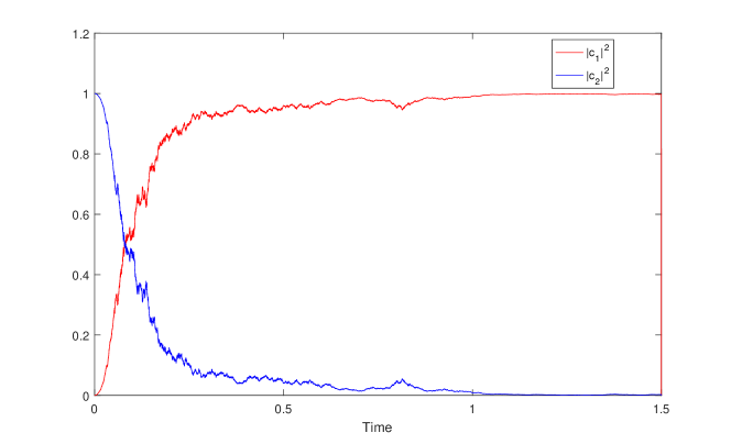
Figure 1: Transition probabilities. The system rotates from $\left|\downarrow\right\rangle$ to $\left|\uparrow\right\rangle$. As it is shown, the proposed control algorithm drives the stochastic system, asymptotically from the initial state to the desired final state. This figure illustrates how this algorithm is useful in order to design controlled quantum gates. This is an example of simple CNOT gate.

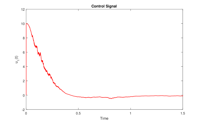
Figure 2: Control signal $u_{1}(t)$. At the beginning, the control effort is high in order to decrease the Lyapunov value. Also, the effect of quantum jumps are substantial in the meanwhile, this is because at the beginning and the end of the transition, the quantum states are eigenkets of $X$.

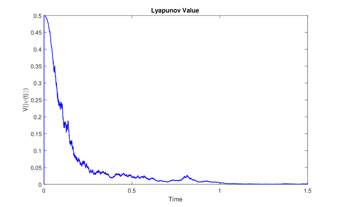
Figure 3: Lyapunov value $V(\left|\psi(t)\right\rangle)$. The Lyapunov value is increasing stochastically as predicted. Also, the asymptotic stability ensures no invariant set in the meanwhile.

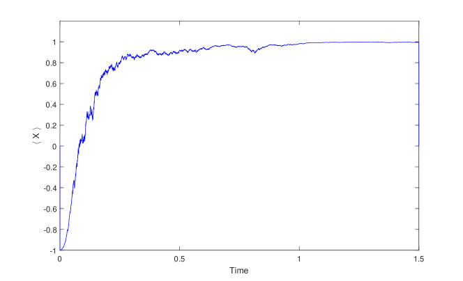
Figure 4: Expectation value $\left\langle X\right\rangle$. This is also the measurement record and shows the extracted information about the state of the system.

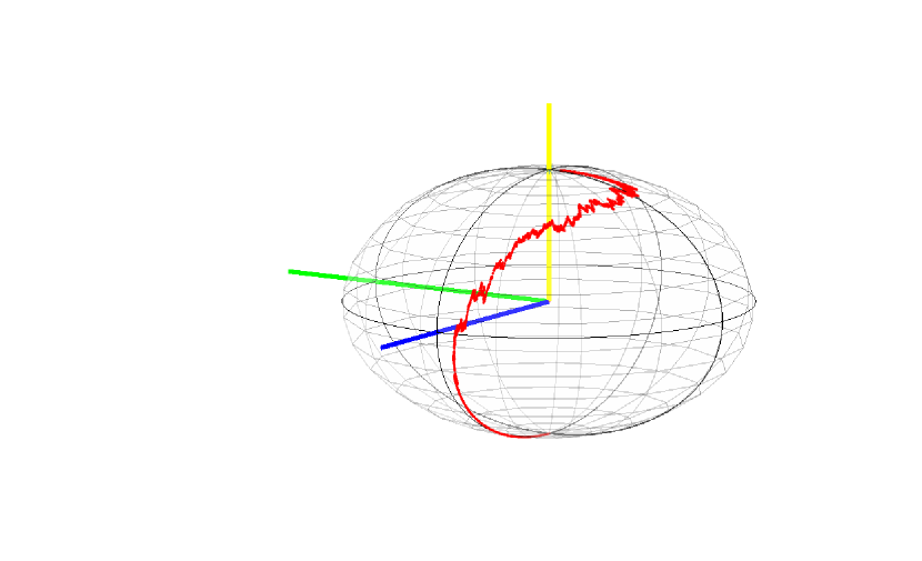
Figure 5: A simple path of state tractores on the Bloch sphere. Yellow, blue and green axes are $Z+$, $Y+$ and $X+$ respectively. The simple path transfers from $\left|\downarrow\right\rangle$ to $\left|\uparrow\right\rangle$. Quantum jumps in the meanwhile are illustrated.

References

- Aharonov et al. (1988) Yakir Aharonov, David Z Albert, and Lev Vaidman. How the result of a measurement of a component of the spin of a spin-1/2 particle can turn out to be 100. Physical review letters, 60(14):1351, 1988.
- Breuer and Petruccione (2002) Heinz-Peter Breuer and Francesco Petruccione. The theory of open quantum systems. Oxford University Press on Demand, 2002.
- Brun (2002) Todd A Brun. A simple model of quantum trajectories. American Journal of Physics, 70(7):719–737, 2002.
- Busch (2009) Paul Busch. No information without disturbance: Quantum limitations of measurement. In Quantum Reality, Relativistic Causality, and Closing the Epistemic Circle, pages 229–256. Springer, 2009.
- Cardona et al. (2018) Gerardo Cardona, Alain Sarlette, and Pierre Rouchon. Exponential stochastic stabilization of a two-level quantum system via strict lyapunov control. In 2018 IEEE Conference on Decision and Control (CDC), pages 6591–6596. IEEE, 2018.
- Cardona et al. (2020) Gerardo Cardona, Alain Sarlette, and Pierre Rouchon. Exponential stabilization of quantum systems under continuous non-demolition measurements. Automatica, 112:108719, 2020.
- Chen et al. (1995) Goong Chen, Guanrong Chen, and Shih-Hsun Hsu. Linear stochastic control systems, volume 3. CRC press, 1995.
- d’Alessandro (2007) Domenico d’Alessandro. Introduction to quantum control and dynamics. CRC press, 2007.
- DiVincenzo (1995) David P DiVincenzo. Quantum computation. Science, 270(5234):255–261, 1995.
- Doob (1953) Joseph L Doob. Stochastic processes, volume 7. Wiley New York, 1953.
- Dowling and Milburn (2003) Jonathan P Dowling and Gerard J Milburn. Quantum technology: the second quantum revolution. Philosophical Transactions of the Royal Society of London A: Mathematical, Physical and Engineering Sciences, 361(1809):1655–1674, 2003.
- Feynman (1982) Richard P Feynman. Simulating physics with computers. International journal of theoretical physics, 21(6):467–488, 1982.
- Ghaeminezhad and Cong (2018) Nourallah Ghaeminezhad and Shuang Cong. Preparation of hadamard gate for open quantum systems by the lyapunov control method. IEEE/CAA Journal of Automatica Sinica, 5(3):733–740, 2018.
- Grivopoulos and Bamieh (2003) Symeon Grivopoulos and Bassam Bamieh. Lyapunov-based control of quantum systems. In Decision and Control, 2003. Proceedings. 42nd IEEE Conference on, volume 1, pages 434–438. IEEE, 2003.
- Gross et al. (2018) Jonathan A Gross, Carlton M Caves, Gerard J Milburn, and Joshua Combes. Qubit models of weak continuous measurements: markovian conditional and open-system dynamics. Quantum Science and Technology, 3(2):024005, 2018.
- Jacobs (2014) Kurt Jacobs. Quantum measurement theory and its applications. Cambridge University Press, 2014.
- Jacobs and Steck (2006) Kurt Jacobs and Daniel A Steck. A straightforward introduction to continuous quantum measurement. Contemporary Physics, 47(5):279–303, 2006.
- Jie et al. (2018) WEN Jie, SHI Yuanhao, and LU Xiaonong. Stabilizing a class of mixed states for stochastic quantum systems via switching control. Journal of the Franklin Institute, 355(5):2562–2582, 2018.
- Jozsa (2007) Richard Jozsa. Complex weak values in quantum measurement. Physical Review A, 76(4):044103, 2007.
- Khalil (1996) Hassan K Khalil. Noninear systems. Prentice-Hall, New Jersey, 2(5):5–1, 1996.
- Khasminskii (2011) Rafail Khasminskii. Stochastic stability of differential equations, volume 66. Springer Science & Business Media, 2011.
- Kuang and Cong (2008) Sen Kuang and Shuang Cong. Lyapunov control methods of closed quantum systems. Automatica, 44(1):98–108, 2008.
- Kuang et al. (2018) Sen Kuang, Daoyi Dong, and Ian R Petersen. Lyapunov control of quantum systems based on energy-level connectivity graphs. IEEE Transactions on Control Systems Technology, 2018.
- Kushner (1967) Harold J Kushner. Stochastic stability and control. Technical report, BROWN UNIV PROVIDENCE RI, 1967.
- Liu et al. (2019) Yanan Liu, Daoyi Dong, Ian R Petersen, and Hidehiro Yonezawa. Filter-based feedback control for a class of markovian open quantum systems. IEEE Control Systems Letters, 3(3):565–570, 2019.
- Mirrahimi et al. (2005) Mazyar Mirrahimi, Pierre Rouchon, and Gabriel Turinici. Lyapunov control of bilinear schrödinger equations. Automatica, 41(11):1987–1994, 2005.
- Muhonen et al. (2018) JT Muhonen, JP Dehollain, A Laucht, S Simmons, R Kalra, FE Hudson, AS Dzurak, A Morello, DN Jamieson, JC McCallum, et al. Coherent control via weak measurements in p 31 single-atom electron and nuclear spin qubits. Physical Review B, 98(15):155201, 2018.
- Pfender et al. (2019) Matthias Pfender, Ping Wang, Hitoshi Sumiya, Shinobu Onoda, Wen Yang, Durga Bhaktavatsala Rao Dasari, Philipp Neumann, Xin-Yu Pan, Junichi Isoya, Ren-Bao Liu, et al. High-resolution spectroscopy of single nuclear spins via sequential weak measurements. Nature communications, 10(1):594, 2019.
- Prugovecki (1982) Eduard Prugovecki. Quantum mechanics in Hilbert space, volume 92. Academic Press, 1982.
- Qamar and Cong (2019) Shahid Qamar and Shuang Cong. Observer-based feedback control of two-level open stochastic quantum system. Journal of the Franklin Institute, 356(11):5675–5691, 2019.
- Ran et al. (2019) Du Ran, Zhi-Cheng Shi, Zhen-Biao Yang, Jie Song, and Yan Xia. Error correction of quantum system dynamics via measurement–feedback control. Journal of Physics B: Atomic, Molecular and Optical Physics, 52(16):165501, 2019.
- Renner (2008) Renato Renner. Security of quantum key distribution. International Journal of Quantum Information, 6(01):1–127, 2008.
- Sastry (2013) Shankar Sastry. Nonlinear systems: analysis, stability, and control, volume 10. Springer Science & Business Media, 2013.
- Shojaee et al. (2018) Ezad Shojaee, Christopher S Jackson, Carlos A Riofrío, Amir Kalev, and Ivan H Deutsch. Optimal pure-state qubit tomography via sequential weak measurements. Physical review letters, 121(13):130404, 2018.
- Shor (1999) Peter W Shor. Polynomial-time algorithms for prime factorization and discrete logarithms on a quantum computer. SIAM review, 41(2):303–332, 1999.
- Shuang and KUANG (2007) Cong Shuang and Sen KUANG. Quantum control strategy based on state distance. Acta Automatica Sinica, 33(1):28–31, 2007.
- Sontag (2013) Eduardo D Sontag. Mathematical control theory: deterministic finite dimensional systems, volume 6. Springer Science & Business Media, 2013.
- Vijay et al. (2012) R Vijay, Chris Macklin, DH Slichter, SJ Weber, KW Murch, Ravi Naik, Alexander N Korotkov, and Irfan Siddiqi. Stabilizing Rabi oscillations in a superconducting qubit using quantum feedback. Nature, 490(7418):77–80, 2012.
- Viola et al. (1999) Lorenza Viola, Emanuel Knill, and Seth Lloyd. Dynamical decoupling of open quantum systems. Physical Review Letters, 82(12):2417, 1999.
- Wang et al. (2014) LC Wang, SC Hou, XX Yi, Daoyi Dong, and Ian R Petersen. Optimal lyapunov quantum control of two-level systems: Convergence and extended techniques. Physics Letters A, 378(16-17):1074–1080, 2014.
- Wang and Schirmer (2010) Xiaoting Wang and Sophie G Schirmer. Analysis of Lyapunov method for control of quantum states. IEEE Transactions on Automatic control, 55(10):2259–2270, 2010.
- Wiseman (1994) HM Wiseman. Quantum theory of continuous feedback. Physical Review A, 49(3):2133, 1994.
- Wiseman (1996) HM Wiseman. Quantum trajectories and quantum measurement theory. Quantum and Semiclassical Optics: Journal of the European Optical Society Part B, 8(1):205, 1996.