Propagation of a Three-dimensional Weak Shock Front Using Kinematical Conservation Laws

Abstract.

In this paper we present a mathematical theory and a numerical method to study the propagation of a three-dimensional (3-D) weak shock front into a polytropic gas in a uniform state and at rest, though the method can be extended to shocks moving into nonuniform flows. The theory is based on the use of 3-D kinematical conservation laws (KCL), which govern the evolution of a surface in general and a shock front in particular. The 3-D KCL, derived purely on geometrical considerations, form an under-determined system of conservation laws. In the present paper the 3-D KCL system is closed by using two appropriately truncated transport equations from an infinite hierarchy of compatibility conditions along shock rays. The resulting governing equations of this KCL based 3-D shock ray theory, leads to a weakly hyperbolic system of eight conservation laws with three divergence-free constraints. The conservation laws are solved using a Godunov-type central finite volume scheme, with a constrained transport technique to enforce the constraints. The results of extensive numerical simulations reveal several physically realistic geometrical features of shock fronts and the complex structures of kink lines formed on them. A comparison of the results with those of a weakly nonlinear wavefront shows that a weak shock front and a weakly nonlinear wavefront are topologically same. The major important differences between the two are highlighted in the contexts of corrugational stability and converging shock fronts.

1. Introduction

A very attractive method for the calculation of successive positions of a shock front is to develop a theory in which we can find the shock strength, position and geometry of the shock at any time without calculating the solution behind the shock. This is a difficult task, because the nonlinear waves which follow the shock strongly influence its evolution. Whitham [31] developed a simple and wonderful approximate method, called the geometrical shock dynamics, in which the effect of the flow behind the shock did not play any role. However, it is well known that the fluid flow behind the shock has an important effect on the shock motion and changes its strength, and this effect has to be correctly accounted. Grinfel’d [12] and Maslov [17] independently showed that the effect on the shock due to the solution behind it can be described in the form of an infinite system of transport equations for the normal derivatives of various orders of a state variable behind the shock. This infinite system of equations is obtained along the shock rays; see [21] for more details of shock rays. Nevertheless, these transport equations turn out to be quite involved and even for a weak shock, when the equations simplify considerably, it is not easy to deal with an infinite system of equations. As a remedy, Prasad and Ravindran [26] proposed a procedure to truncate the infinite system and thus developed the new theory of shock dynamics (NTSD). The governing equations in this theory form a coupled set of differential equations, consisting of the ray equations and those obtained by truncating the infinite system. It is quite simple to use the NTSD to one-dimensional (1-D) shock propagation, but its application to multidimensional problems remained a challenge due to the formation of kink (explained in the next two paragraphs) type of singularities, which are found very frequently on a shock front. The appearance of kinks were observed also in the numerical simulations of a nonlinear wavefront; see [25] for more details. The kinks are formed on these fronts due to self-focusing. The first experimental results showing the formation of kinks on a shock front are available in the work of Sturtevant and Kulkarny [29]. These authors reported that the kinks appear on a focusing shock front which is not too weak and it remained a challenge to reproduce their experimental results by an analytical method. However, Kevlahan [14] used the NTSD to study this problem and his numerical results agreed well not only with the experimental results but also with some known exact and numerical solutions of the Euler equations. This clearly shows the efficacy of NTSD to produce physically realistic results.

A kink (kink line) is a point (curve) on a moving curve (surface), across which the normal direction to the curve (surface) suffers a jump discontinuity. The formation and propagation of kinks on a shock front and also a nonlinear wavefront necessitated a conservative formulation of the equations of NTSD as well as the equations governing the motion of a weakly nonlinear wavefront. This requirement finally led to the development of the kinematical conservation laws (KCL) for the evolution of a curve in a plane by Morton et al. [19] and for a surface in three-dimensional (3-D) space by Giles et al. [11].

For the sake of completeness and to make this paper self-contained, in the following we briefly review the some basic results from [2, 4]. The $d$-dimensional KCL is a system of conservation equations governing the evolution of a surface $\Omega_{t}$ in $\mathbb{R}^{d}$. The KCL is derived in specially defined ray coordinates $(\xi_{1},\xi_{2},\ldots,\xi_{d-1},t)$, where $\xi_{1},\xi_{2},\ldots,\xi_{d-1}$ are the surface coordinates on $\Omega_{t}$ and $t$ is time. The mapping between the ray coordinates $(\xi_{1},\xi_{2},\ldots,\xi_{d-1},t)$ and the spatial coordinates $(x_{1},x_{2},\ldots,x_{d})$ is assumed to be locally one-to-one. Since the KCL is a system of conservation laws, its solutions may contain shocks in the ray coordinates. An image of any one of these shocks, when mapped onto the $(x_{1},x_{2},\ldots,x_{d})$-space, is a kink surface on $\Omega_{t}$ across which the normal direction to $\Omega_{t}$ and normal velocity are discontinuous. Hence, the KCL is ideally suited to study the evolution of a surface having kink type of singularities. However, the KCL being purely a geometric result, it forms an incomplete system of equations and additional closure relations are necessary to get a completely determined set of equations. When $\Omega_{t}$ is a weakly nonlinear wavefront in a polytropic gas [20], the KCL system is closed by a single equation representing the conservation of total energy in a ray tube; see [3, 4] for more details. Throughout this paper we shall refer to the resulting complete system of conservation laws, governing the evolution of a nonlinear wavefront, as KCL based weakly nonlinear ray theory (WNLRT), or briefly 3-D WNLRT in later sections. In the 2-D case this system consists of just three conservation laws in $(\xi_{1},t)$ coordinates, which is hyperbolic when an appropriately defined non-dimensional front velocity $m>1$; see [22]. In the case of a polytropic gas, $m>1$ corresponds to a wavefront on which the pressure is greater than the constant pressure in the ambient gas. However, the simplicity of 2-D KCL is lost when we consider the 3-D KCL, which is a system of six conservation laws in $(\xi_{1},\xi_{2},t)$ coordinates with three stationary divergence-free constraints. Following [2], we shall refer to these three constraints together as “geometric solenoidal constraint”. The KCL based 3-D WNLRT consists of seven equations and unlike the 2-D case, this system is only weakly hyperbolic for $m>1$, in the sense that it has two distinct eigenvalues and an eigenvalue of multiplicity five with a four-dimensional eigenspace [4, 5].

The eigenvalues of KCL based 3-D WNLRT are all real when $m>1$. However, the weakly hyperbolic nature of the system and the presence of geometric solenoidal constraint pose a challenge to develop a numerical approximation. It is well known from the literature that when the dimension of the eigenspace corresponding to a multiple eigenvalue has a deficiency of one, the solution to a Cauchy problem contains a mode, the so-called “Jordan mode”, which grows linearly in time. However, it has been shown in [2] that when the geometric solenoidal constraint is satisfied initially, the solution to a Cauchy problem does not exhibit the Jordan mode. Motivated by this, in [2], a constraint transport (CT) technique has been built into a central finite volume scheme for the 3-D WNLRT system, therein the constraint is maintained up to machine accuracy with the elimination of the Jordan mode. In addition, the numerical method is shown to be very robust, second order accurate and the numerical solution can be continued for a very long time, almost indefinitely.

In [7, 18] the authors have proposed a conservative formulation of the NTSD based on 2-D KCL and it turned out to be more effective than using the NTSD in a differential form as done in [14]. A conservative formulation also has the advantage of using modern shock-capturing algorithms and hence the kinks, whenever formed on the shock in $(x_{1},x_{2})$-plane, can be automatically tracked as the images of shocks in the ray coordinates $(\xi_{1},t)$. The goal of the present work is to derive the conservation laws of NTSD for a weak shock based on the 3-D KCL and to use them for the computation of 3-D shock fronts. We shall designate the conservation laws thus obtained as the KCL based 3-D shock ray theory, or simply in 3-D SRT throughout this paper. Our contribution consists in formulation and analysis of 3-D SRT, its numerical approximation and the results of numerical experiments. These results reveal many realistic geometrical features of shock fronts, the complex structure of kink lines and a comparison with those in [2] shows that a weak shock front and weakly nonlinear wavefront are topologically the same.

The rest of this paper is organised as follows. In section 2 we derive the system of conservation laws of 3-D SRT and analyse its eigen-structure. In section 3 we briefly formulate a numerical approximation of 3-D SRT, based on the constraint preserving, high resolution central finite volume scheme from [2]. The results of numerical case studies are presented in section 4 and in order to facilitate the comparison, the initial data for these tests are chosen as in [2]. In those test cases, where we observe the results qualitatively similar to those in [2], we refrain from presenting detailed and lengthy inferences. However, in a test problem in which the interactions of kink lines and the corrugational stability of a shock front are clearly observed, we present a thorough analysis. In this case, as well as in the case of a radially converging shock front, we highlight the important differences between a weak shock front and a weakly nonlinear wavefront. Finally, we close this paper with some concluding remarks in section 5.

2. Governing Equations of 3-D SRT

A system of shock ray equations consists of the ray equations derived from a shock manifold partial differential equation [21] and an infinite system of compatibility conditions along a shock ray [1, 12, 17, 28]. These compatibility conditions are derived from the equations governing the motion of the medium in which the shock propagates, e.g. the Euler equations of gas dynamics. It has to be noted that unlike the well known geometric optics theory for the propagation of a one-parameter family of wavefronts, across which wave amplitudes are continuous, the SRT with an infinite system of compatibility conditions is exact. This is because the high frequency approximation required for the derivation of jump relations is exactly satisfied for a shock front.

Let us consider a shock propagating into a polytropic gas at rest and in a uniform state $(\varrho,\mbox{\boldmath$q$},p)=(\varrho_{0},\mbox{\boldmath$0$},p_{0})$, where $\varrho$ is the density, $\mbox{\boldmath$q$}=(q_{1},q_{2},q_{3})$ is the particle velocity and $p$ is the pressure. Let $a$ be the sound velocity in the medium defined by $a^{2}=\gamma p/\varrho$, where $\gamma$ is the ratio of specific heats. Let $N$ denotes the unit normal to the shock. Assuming the shock to be weak, the small amplitude perturbations in the density $\varrho$, fluid velocity $q$ and pressure $p$ up to a short distance behind the shock can be expressed using a small parameter $\varepsilon$ via the relations [22]

(2.1) $$\varrho-\varrho_{0}=\varepsilon\frac{\varrho_{0}}{a_{0}}\tilde{w},\ \mbox{\boldmath$q$}=\varepsilon\tilde{w}\mbox{\boldmath$N$},\ p-p_{0}=\varepsilon\varrho_{0}a_{0}\tilde{w},$$

where $a_{0}$ is the sound speed in the uniform state and $\tilde{w}$ is an amplitude of the order of unity, having the dimension of velocity. Let us introduce a non-dimensional amplitude $\mu$, defined on the shock front, via

(2.2) $$\mu:=\left.\frac{\tilde{w}}{a_{0}}\right|_{s}.$$

Following [18, 22], it can easily be seen that a point $\mbox{\boldmath$X$}=(X_{1},X_{2},X_{3})$ on a shock ray satisfies

(2.3) $$\frac{\mathrm{d}\mbox{\boldmath$X$}}{\mathrm{d}T} =a_{0}\left(1+\varepsilon\frac{\gamma+1}{4}\mu\right)\mbox{\boldmath$N$},$$

(2.4) $$\frac{\mathrm{d}\mbox{\boldmath$N$}}{\mathrm{d}T} =-\varepsilon\frac{\gamma+1}{4}a_{0}\mbox{\boldmath$L$}\mu,$$

where $\mathrm{d}/\mathrm{d}T$ denotes the derivative

(2.5) $$\frac{\mathrm{d}}{\mathrm{d}T}:=\frac{\partial}{\partial t}+a_{0}\left(1+\varepsilon\frac{\gamma+1}{4}\mu\right)\langle\mbox{\boldmath$N$},\nabla\rangle$$

and $L$ is a tangential derivative along the shock front, defined by

(2.6) $$\mbox{\boldmath$L$}:=\nabla-\mbox{\boldmath$N$}\langle\mbox{\boldmath$N$},\nabla\rangle.$$

For a weak shock, the first two of the infinite system of compatibility conditions along the shock rays (2.3)-(2.4) are given by [22]

(2.7) $$\frac{\mathrm{d}\mu}{\mathrm{d}T} =a_{0}{\it\Omega}_{s}\mu-\frac{\gamma+1}{4}\mu\mu_{1},$$

(2.8) $$\frac{\mathrm{d}\mu_{1}}{\mathrm{d}T} =a_{0}{\it\Omega}_{s}\mu_{1}-\frac{\gamma+1}{2}\mu_{1}^{2}-\frac{\gamma+1}{4}\mu\mu_{2}.$$

At this point, we caution the reader that the coefficient of $\mu_{1}^{2}$ in (2.8) has a misprint in the references [18, 22]. The term ${\it\Omega}_{s}$ in (2.7)-(2.8) denotes the mean curvature of the shock and the variables $\mu_{1}$ and $\mu_{2}$ are defined by

(2.9) $$\mu_{1}:=\varepsilon\left.\langle\mbox{\boldmath$N$},\nabla\rangle\tilde{w}\right|_{s},\ \mu_{2}:=\varepsilon^{2}\left.\langle\mbox{\boldmath$N$},\nabla\rangle^{2}\tilde{w}\right|_{s}.$$

Due to the short wave approximation, both the quantities $\mu_{1}$ and $\mu_{2}$ are of order unity [18, 22]. The effect of the term $\mu_{1}$ is very important in shock propagation. It represents the gradient in the normal direction of the pressure or density just behind the shock and takes into account of the effect of interactions of the nonlinear waves which catch the shock from behind. It has to be noted that apart from (2.7)-(2.8), there exists an infinite system of compatibility conditions for properly defined higher order derivatives $\mu_{2},\mu_{3},\mu_{4},\ldots$ on the shock. However, it appears to be very difficult to use this infinite system of coupled equations for computing shock propagation.

The idea behind NTSD is to drop the term containing $\mu_{2}$ in (2.8); see [26]. Once this is done, the system of equations (2.3)-(2.4) and (2.7)-(2.8) is closed and it can then used to compute shock propagation. For a discussion on the validity of NTSD and its application to 2-D problems we refer the reader to [7, 14, 18, 22]. It is interesting to note that the NTSD gives quite good results even for a shock of arbitrary strength, which has been verified for a 1-D piston problem in [16]. In addition, it has also been observed in [16] that the NTSD takes less than $0.5\%$ of the computational time needed by a typical finite difference method applied to the Euler equations.

2.1. Conservation Forms of the Governing Equations

As a first step, we non-dimensionalise all the independent and dependent variables with the help of a characteristic length $L$ and the sound velocity $a_{0}$ in the uniform medium ahead of the shock. We continue to denote all the resulting non-dimensional variables also by the same symbols. Here, we choose $L$ to be of the order of the distance over which the SRT is valid and also the distance over which the shock propagates. It has to be noted that the nonlinear theory of Choquet-Bruhat [9] is valid over a distance smaller than the smaller of the radii of curvatures of the front at $t=0$. However, for WNLRT and SRT, the distance $L$ could be far beyond the caustic region as evident from the numerical results presented in [3, 7, 18, 24].

We now proceed to derive a conservation form the equations (2.3)-(2.4) and (2.7)-(2.8). Let us define two variables $M$ and $\mathcal{V}$ via

(2.10) $$M:=1+\varepsilon\frac{\gamma+1}{4}\mu,\ \mathcal{V}:=\frac{\gamma+1}{4}\mu_{1}.$$

Here, $M$ is a non-dimensional Mach number of the shock front and $\mathcal{V}$ is an appropriately scaled normal derivative of the gas density or pressure, just behind the shock. Following NTSD, we drop the last term containing $\mu_{2}$ in (2.8) and rewrite (2.7)-(2.8) in terms of $M$ and $\mathcal{V}$ to obtain

(2.11) $$\frac{\mathrm{d}M}{\mathrm{d}T} ={\it\Omega}_{s}(M-1)-\mathcal{V}(M-1),$$

(2.12) $$\frac{\mathrm{d}\mathcal{V}}{\mathrm{d}T} ={\it\Omega}_{s}\mathcal{V}-2\mathcal{V}^{2}.$$

We introduce a ray coordinate system $(\xi_{1},\xi_{2},t)$ on the shock front in such a way that $t=\mathrm{const}$ is the shock front $\Omega_{t}$ and ($\xi_{1}=\mathrm{const},\xi_{2}=\mathrm{const}$) is a two-parameter family of rays in the $(x_{1},x_{2},x_{3})$-space. Let $U$ and $V$ be respectively the unit tangent vectors along the curves ($\xi_{2}=\mathrm{const},t=\mathrm{const}$) and ($\xi_{1}=\mathrm{const},t=\mathrm{const}$) on $\Omega_{t}$. We denote by $G_{1}$ and $G_{2}$ respectively, the associated metrics. On a given shock front at any time $t$ we have the relations

(2.13) $$\mbox{\boldmath$X$}_{\xi_{1}}=G_{1}\mbox{\boldmath$U$},\ \mbox{\boldmath$X$}_{\xi_{2}}=G_{2}\mbox{\boldmath$V$},$$

where $G_{1}$ and $G_{2}$ are given by $G_{1}=\lVert\mbox{\boldmath$X$}_{\xi_{1}}\rVert$ and $G_{2}=\lVert\mbox{\boldmath$X$}_{\xi_{2}}\rVert$. In view of the definition of $M$ from (2.10), in non-dimensional coordinates, the derivative $\mathrm{d}/\mathrm{d}T$ defined in (2.5) assumes the form

(2.14) $$\frac{\mathrm{d}}{\mathrm{d}T}=\frac{\partial}{\partial t}+M\langle\mbox{\boldmath$N$},\nabla\rangle$$

and it represents the time rate of change along a shock ray. Hence, in the ray coordinates $(\xi_{1},\xi_{2},t)$, the derivative $\mathrm{d}/\mathrm{d}T$ simply becomes $\partial/\partial t$.

As in [4] it can be shown that the first and second part of the ray equations, namely (2.3)-(2.4), are equivalent to the 3-D KCL

(2.15) $$(G_{1}\mbox{\boldmath$U$})_{t}-(M\mbox{\boldmath$N$})_{\xi_{1}} =0,$$

(2.16) $$(G_{2}\mbox{\boldmath$V$})_{t}-(M\mbox{\boldmath$N$})_{\xi_{2}} =0$$

with the constraint

(2.17) $$(G_{2}\mbox{\boldmath$V$})_{\xi_{1}}-(G_{1}\mbox{\boldmath$U$})_{\xi_{2}}=0.$$

Therefore, it only remains to derive a conservation form of the transport equations (2.11)-(2.12). Our approach is along the lines of [23] which follow a general pattern valid for all compatibility conditions; see also [7].

The ray tube area $\mathcal{A}$ of a tube of shock rays [22, 31] is related to the mean curvature ${\it\Omega}_{s}$ by the relation

(2.18) $$\frac{1}{\mathcal{A}}\frac{\mathrm{d}\mathcal{A}}{\mathrm{d}l}=-2{\it\Omega}_{s},$$

where $l$ denotes the length measured along a shock ray. In non-dimensional variables we have $\mathrm{d}l=M\mathrm{d}T$ and therefore from (2.18) we get

(2.19) $${\it\Omega}_{s}=-\frac{1}{2M\mathcal{A}}\frac{\mathrm{d}\mathcal{A}}{\mathrm{d}T}.$$

We notice the presence of the term ${\it\Omega}_{s}$ in both the transport equations (2.11) and (2.12). In the light of (2.19), we conclude that ${\it\Omega}_{s}$ is related to the rate of change of the ray tube area, viz. $\mathrm{d}\mathcal{A}/\mathrm{d}T$. Therefore, this term in the equations (2.11)-(2.12) represents the geometric decay or amplification of the quantities $M$ and $\mathcal{V}$ .

We use the relation (2.19) in (2.11) with $\mathrm{d}/\mathrm{d}T$ replaced by $\partial/\partial t$ in the ray coordinates and obtain

(2.20) $$\frac{2M}{M-1}M_{t}+\frac{\mathcal{A}_{t}}{\mathcal{A}}+2M\mathcal{V}=0.$$

Note that the left hand side of the above equation gives a combination $\{f^{\prime}(h)/f(h)\}h_{t}+\mathcal{A}_{t}/\mathcal{A}$, where $h=M-1$ and $f$ is the function $f(h):=h^{2}e^{2h}$. Hence, we get a conservation form

(2.21) $$\left\{\mathcal{A}f(M-1)\right\}_{t}+2\mathcal{A}Mf(M-1)\mathcal{V}=0.$$

The ray tube area $\mathcal{A}$ is given by the expression

(2.22) $$\mathcal{A}=G_{1}G_{2}\sin\Psi,$$

where $\Psi$ is the angle between the two unit vectors $U$ and $V$. Therefore, from (2.21), we finally get a balance equation

(2.23) $$\left\{(M-1)^{2}e^{2(M-1)}G_{1}G_{2}\sin\Psi\right\}_{t}+2M(M-1)^{2}e^{2(M-1)}G_{1}G_{2}\mathcal{V}\sin\Psi=0.$$

Similarly, using the expression (2.19) for ${\it\Omega}_{s}$ in (2.12) we obtain an equation which we rewrite as

(2.24) $$\mathcal{V}_{t}+\frac{\mathcal{V}}{2\mathcal{A}}\mathcal{A}_{t}+\frac{\mathcal{V}}{2}\left(\frac{1}{M}-1\right)\frac{\mathcal{A}_{t}}{\mathcal{A}}+2\mathcal{V}^{2}=0.$$

We use (2.20) to replace the factor $\mathcal{A}_{t}/\mathcal{A}$ from the third term in (2.24) and write the resulting equation as

(2.25) $$\left\{\ln\left(\mathcal{V}^{2}\mathcal{A}\right)+2(M-1)\right\}_{t}+(M+1)\mathcal{V}=0,$$

which gives a balance equation

(2.26) $$\left\{e^{2(M-1)}G_{1}G_{2}\mathcal{V}^{2}\sin\Psi\right\}_{t}+(M+1)e^{2(M-1)}G_{1}G_{2}\mathcal{V}^{3}\sin\Psi=0.$$

Remark 2.1.

The second term in (2.20) and the second and third terms in (2.24) represent the geometrical effect of convergence or divergence of rays. The third term in (2.20) represents the effect of interaction of nonlinear waves which overtake the shock from behind. The fourth term in (2.24) is the usual effect of genuine nonlinearity which governs the evolution of $\mathcal{V}$, also seen in the 1-D model $u_{t}+uu_{x}=0$.

The complete set of equations of 3-D KCL based NTSD, hereafter designated as the conservation laws of 3-D SRT, consists of the equations (2.15)-(2.16), (2.23) and (2.26).

Remark 2.2.

The conservation forms the (2.23) and (2.26) of the compatibility conditions (2.11) and (2.12) respectively, are physically realistic. They are the three-dimensional extensions of those derived by Baskar and Prasad [7], namely

(2.27) $$\left\{(M-1)^{2}e^{2(M-1)}G\right\}_{t}+2M(M-1)^{2}e^{2(M-1)}G\mathcal{V} =0,$$

(2.28) $$\left\{e^{2(M-1)}G\mathcal{V}^{2}\right\}_{t}+(M+1)e^{2(M-1)}G\mathcal{V}^{3} =0.$$

Note that (2.27) and (2.28) follow from (2.23) and (2.26) respectively, by replacing $G_{1}G_{2}\sin\Psi$ by $G$. In the linear theory, the energy conservation along a ray tube is represented by $\{G(M-1)^{2}\}_{t}=0$, which can be written in an integral formulation using two cross-sections of a ray tube; see [31]. The genuine nonlinearity in Euler equations stretches a shock ray (i.e., makes the shock front move faster) due to presence of the term $M\langle\mbox{\boldmath$N$},\nabla\rangle$ in (2.14) and hence the flux of energy across a section of a shock ray tube increases by a factor $e^{2(M-1)}$. Though this term looks small for a weak shock, its accumulative effect over long time is significant. Presence of this term is also seen in the conservation laws of 3-D WNLRT in [4]. The source term in (2.23), leading to a decay in the shock velocity when $\mathcal{V}>0$, is the main cause of differences in the results as compared to the results for a nonlinear wavefront. We shall postpone a detailed discussion on this to section 4.

One of the aims of this paper is to compare the the results of 3-D SRT with those of 3-D WNLRT, reported in [2]. Hence, for the sake of completeness, in the following we reproduce the conservation laws 3-D WNLRT, i.e.

(2.29) $$(g_{1}\mbox{\boldmath$u$})_{t}-(m\mbox{\boldmath$n$})_{\xi_{1}} =0,$$

(2.30) $$(g_{2}\mbox{\boldmath$v$})_{t}-(m\mbox{\boldmath$n$})_{\xi_{2}} =0,$$

(2.31) $$\left((m-1)^{2}e^{2(m-1)}g_{1}g_{2}\sin\psi\right)_{t} =0$$

with the constraint

(2.32) $$(g_{2}\mbox{\boldmath$v$})_{\xi_{1}}-(g_{1}\mbox{\boldmath$u$})_{\xi_{2}}=0.$$

We notice that unlike the balance equations of 3-D SRT, the system of conservation laws (2.29)-(2.31) is homogeneous, i.e. without any source term.

2.2. Eigen-structure of the System of Conservation Laws

This section is devoted to the analysis of the eigenvalues and eigenvectors of the system conservations laws (2.15)-(2.16), (2.23) and (2.26). First, we recast them in the usual divergence form

(2.33) $$W_{t}+{F_{1}(W)}_{\xi_{1}}+{F_{2}(W)}_{\xi_{2}}=S(W)$$

with the conserved variable $W$, the fluxes $F_{1}(W),F_{2}(W)$ and the source term $S(W)$, given as

(2.34) $$W =\left(G_{1}\mbox{\boldmath$U$},G_{2}\mbox{\boldmath$V$},(M-1)^{2}e^{2(M-1)}G_{1}G_{2}\sin\Psi,e^{2(M-1)}G_{1}G_{2}\mathcal{V}^{2}\sin\Psi\right)^{T},$$

$$F_{1}(W) =\left(M\mbox{\boldmath$N$},\mbox{\boldmath$0$},0,0\right)^{T},$$

$$F_{2}(W) =\left(\mbox{\boldmath$0$},M\mbox{\boldmath$N$},0,0\right)^{T},$$

$$S(W) =\left(\mbox{\boldmath$0$},\mbox{\boldmath$0$},-2M(M-1)^{2}e^{2(M-1)}G_{1}G_{2}\mathcal{V}\sin\Psi,-(M+1)e^{2(M-1)}G_{1}G_{2}\mathcal{V}^{3}\sin\Psi\right)^{T}.$$

In order to discuss the eigenvalues and eigen-structure of (2.33), we need its explicit form as a system of partial differential equations. Introducing a vector of primitive variables via $V=(U_{1},U_{2},V_{1},V_{2},M,G_{1},G_{2},\mathcal{V})^{T}$, we can derive a quasi-linear form of (2.33) as

(2.35) $$\tilde{A}V_{t}+\tilde{B}^{(1)}V_{\xi_{1}}+\tilde{B}^{(2)}V_{\xi_{2}}=\tilde{C},$$

where the expressions for the matrices $\tilde{A},\tilde{B}^{(1)},\tilde{B}^{(2)}$ and $\tilde{C}$ are given in Appendix A. It is interesting to note that the matrices $\tilde{A},\tilde{B}^{(1)}$ and $\tilde{B}^{(2)}$ admit the following block structure

(2.36) $$\tilde{A}=\begin{pmatrix}A&O_{7,1}\\ R_{1,7}&\frac{2G_{1}G_{2}}{\mathcal{V}}\end{pmatrix},\ \tilde{B}^{(1)}=\begin{pmatrix}B^{(1)}&O_{7,1}\\ O_{1,7}&0\end{pmatrix},\ \tilde{B}^{(2)}=\begin{pmatrix}B^{(2)}&O_{7,1}\\ O_{1,7}&0\end{pmatrix}.$$

Here, $A,B^{(1)}$ and $B^{(2)}$ are the corresponding flux Jacobian matrices of 3-D WNLRT, cf. [3, 4], $O$ denotes a zero-matrix and $R_{1,7}$ is a row-matrix; see also Appendix A. The characteristic equation of (2.35) is given by

(2.37) $$\det\tilde{M}_{8,8}(\lambda)\equiv\det\left(e_{1}\tilde{B}^{(1)}+e_{2}\tilde{B}^{(2)}-\lambda\tilde{A}\right)=0.$$

Using the block structure of the matrices in (2.36) we can obtain

(2.38) $$\tilde{M}_{8,8}(\lambda)=\begin{pmatrix}M_{7,7}(\lambda)&O_{7,1}\\ -\lambda R_{1,7}&-\lambda\frac{2G_{1}G_{2}}{\mathcal{V}}\end{pmatrix},$$

where $M_{7,7}(\lambda):=e_{1}B^{(1)}+e_{2}B^{(2)}-\lambda A$ is the matrix pencil of the 3-D WNLRT. Therefore, the characteristic equation (2.37) simplifies as

(2.39) $$\lambda\det M_{7,7}(\lambda)=0.$$

Using the results of [4, 5], it is easy to find the roots of the polynomial equation $\det M_{7,7}(\lambda)=0$ in $\lambda$ and the nullvectors of $M_{7,7}$ corresponding to these roots. The roots of (2.37) can be obtained as $\lambda_{1},\lambda_{2}(=-\lambda_{1}),\lambda_{3}=\cdots=\lambda_{8}=0$, where

(2.40) $$\lambda_{1}=\left\{\frac{M-1}{2\sin^{2}\Psi}\left(\frac{e_{1}^{2}}{G_{1}^{2}}-\frac{2e_{1}e_{2}}{G_{1}G_{2}}\cos\Psi+\frac{e_{2}^{2}}{G_{2}^{2}}\right)\right\}^{\frac{1}{2}}$$

and $(e_{1},e_{2})\in\mathbb{R}^{2}$ with $e_{1}^{2}+e_{2}^{2}=1$. Let us now consider the matrix $\tilde{M}_{8,8}(0)$ for the multiple eigenvalue $\lambda=0$. Clearly, the rank of the matrix $\tilde{M}_{8,8}(0)$ is same as that of $M_{7,7}(0)$, cf. (2.38). It has been shown in [4] that the rank of $M_{7,7}(0)$ is three. Thus, the dimension of the nullspace of $\tilde{M}_{8,8}(0)$ is $8-3=5$. This proves that the dimension of the eigenspace corresponding to $\lambda=0$ of multiplicity six is only five. We summarise these results as a theorem.

Theorem 2.3.

The system (2.35) has eight eigenvalues $\lambda_{1},\lambda_{2}~{}(=-\lambda_{1}),\lambda_{3}=\lambda_{4}=\cdots=\lambda_{8}=0$, where $\lambda_{1}$ and $\lambda_{2}$ are real for $M>1$ and purely imaginary for $M<1$. Further, the dimension of the eigenspace corresponding to the multiple eigenvalue zero is five.

Remark 2.4.

It is important to note that $M<1$ is not physically unrealistic for a shock. For example, the signature of a sonic boom produced by a convex and smooth upper surface an aerofoil with a sharp leading edge (see figures 2.1 and 2.2, [8]) consists of a leading shock followed by a continuous flow in which the pressure decreases and terminates in a trailing shock. In the forward part of the continuous flow the pressure is greater than that in the ambient medium and in the rear part it is less than that behind the trailing shock. The shock velocity of the trailing weak shock is half of the sound velocity behind it, say $a_{0}$ and the sound speed ahead of it, which is less than $a_{0}$. Thus Mach number $M$ of the trailing shock is less than $1$.

3. Numerical Approximation

As a consequence of Theorem 2.3 we infer that the system of conservation laws (2.33) is only weakly hyperbolic for $M>1$; hence, an initial value problem may not be well-posed in the strong hyperbolic sense. In addition, weakly hyperbolic systems are likely to be more sensitive than regular hyperbolic systems also from a computational point of view. Numerical as well as theoretical analysis indicates that their solution may not belong to the BV spaces and can only be measure valued. Despite such theoretical difficulties, in [2, 3], we have been able to develop accurate and efficient numerical approximations of the analogous weakly hyperbolic system of 3-D WNLRT using, simple but robust, central schemes. Since the conservation laws of 3-D SRT and those of 3-D WNLRT, viz. (2.29)-(2.32), are structurally similar, we do not intend to present the details of the numerical approximation and the refer the reader to [2] for more details.

We discretise the system (2.33) using the cell integral averages $\overline{W}_{i,j}$ of the conservative variable $W$, taken over square mesh cells. From the given cell averages $\overline{W}_{i,j}^{n}$ at time $t^{n}$, we reconstruct a piecewise linear interpolant using the standard MUSCL type procedures. In order to obtain the discrete slopes in the $\xi_{1}$- and $\xi_{2}$-directions, we employ a central weighted essentially non-oscillatory limiter [13]. The piecewise linear reconstruction enables us to compute the cell interface values of the conserved variable $W$.

The starting point for the construction of numerical scheme is a semi-discrete discretisation of (2.33), given by

(3.1) $$\frac{\mathrm{d}\overline{W}_{i,j}}{\mathrm{d}t}=-\frac{{\mathcal{F}_{1}}_{i+\frac{1}{2},j}-{\mathcal{F}_{1}}_{i-\frac{1}{2},j}}{h_{1}}-\frac{{\mathcal{F}_{2}}_{i,j+\frac{1}{2}}-{\mathcal{F}_{2}}_{i,j-\frac{1}{2}}}{h_{2}}+S(\overline{W}_{i,j}),$$

where the quantities $\mathcal{F}_{i+1/2,j}$ and $\mathcal{F}_{i,j+1/2}$ are respectively, the numerical fluxes at the cell interfaces $(i+1/2,j)$ and $(i,j+1/2)$. We employ the high resolution flux given by Kurganov and Tadmor [15], for these interface fluxes, e.g. at a right-hand vertical edge

(3.2) $${\mathcal{F}_{1}}_{i+\frac{1}{2},j}\left(W_{i,j}^{R},W_{i+1,j}^{L}\right)=\frac{1}{2}\left(F_{1}\left(W_{i+1,j}^{L}\right)+F_{1}\left(W_{i,j}^{R}\right)\right)-\frac{a_{i+\frac{1}{2},j}}{2}\left(W_{i+1,j}^{L}-W_{i,j}^{R}\right),$$

where $W_{i,j}^{L(R)}$ denote respectively, the left and right interpolated states at the interface $(i+1/2,j)$. The expression for the flux $\mathcal{F}_{i,j+1/2}$ at an upper horizontal edge is analogous. In the flux formula (3.2), the term $a_{i+1/2,j}$ denotes the local speed of propagation at cell interfaces, given by

(3.3) $$a_{i+\frac{1}{2},j}:=\max\left\{\rho\left(\frac{\partial F_{1}}{\partial W}\left(W_{i,j}^{R}\right)\right),\rho\left(\frac{\partial F_{1}}{\partial W}\left(W_{i+1,j}^{L}\right)\right)\right\}$$

where $\rho(A):=\max_{i}\lvert\lambda_{i}(A)\rvert$, with $\lambda_{i}(A)$ being the eigenvalues of the matrix $A$.

To improve the temporal accuracy and to gain second order accuracy in time, we use a TVD Runge-Kutta scheme [27] to numerically integrate the system of ordinary differential equations in (3.1). Denoting the right hand side of (3.1) by $\mathcal{L}_{i,j}(W)$, the second order Runge-Kutta scheme updates $W$ through the following two stages

(3.4) $$W_{i,j}^{(1)} =\overline{W}_{i,j}^{n}+\Delta t\mathcal{L}_{i,j}\left(\overline{W}^{n}\right),$$

$$\overline{W}_{i,j}^{n+1} =\frac{1}{2}\overline{W}_{i,j}^{n}+\frac{1}{2}W_{i,j}^{(1)}+\frac{1}{2}\Delta t\mathcal{L}_{i,j}\left(W^{(1)}\right).$$

It is to be noted that any consistent numerical solution of the 3-D KCL system (2.15)-(2.16) also has to satisfy the geometric solenoidal constraint (2.17) at any time. Note that this constraint is an involution for the 3-D KCL (2.15)-(2.16), i.e. once fulfilled at the initial data it is fulfilled for all times. Since the physically exact solution has this feature, a numerical solution should also possess it some discrete sense. Hence, in the numerical approximation of the analogous 3-D WNLRT system in [2], a CT algorithm [10] was built into the central finite volume to enforce the geometric solenoidal constraint. In what follows, we briefly review this CT strategy and refer to [2] for more details on its implementation.

The geometric solenoidal constraint (2.17) guarantees the existence of three potential functions $\mathbb{A}_{k},k=1,2,3$, such that

(3.5) $$G_{1}U_{k}={\mathbb{A}_{k}}_{\xi_{1}},\ G_{2}V_{k}={\mathbb{A}_{k}}_{\xi_{2}}.$$

Using (3.5) in the 3-D KCL system (2.15)-(2.16) yields the evolution equations

(3.6) $${\mathbb{A}_{k}}_{t}=MN_{k}.$$

In the CT method, we store the three potentials $\mathbb{A}_{k}$ at the centres of a staggered grid. With aid of these potentials we redefine the values of the vectors $G_{1}\mbox{\boldmath$U$}$ and $G_{2}\mbox{\boldmath$V$}$ at the cell edges, which are treated as length averaged quantities. In this way, $G_{2}\mbox{\boldmath$V$}$ is collocated at $(i+1/2,j)$, whereas $G_{1}\mbox{\boldmath$U$}$ is collocated at $(i,j+1/2)$. The definitions of these collocated values are obtained by simply discretising the derivatives in (3.5) using central differences, i.e.

(3.7) $$[G_{1}U_{k}]_{i,j+\frac{1}{2}} =\frac{1}{h_{1}}\left({\mathbb{A}_{k}}_{i+\frac{1}{2},j+\frac{1}{2}}-{\mathbb{A}_{k}}_{i-\frac{1}{2},j+\frac{1}{2}}\right),$$

(3.8) $$[G_{2}V_{k}]_{i+\frac{1}{2},j} =\frac{1}{h_{2}}\left({\mathbb{A}_{k}}_{i+\frac{1}{2},j+\frac{1}{2}}-{\mathbb{A}_{k}}_{i+\frac{1}{2},j-\frac{1}{2}}\right).$$

With the above collocated values we calculate

(3.9) $$\left.(G_{2}V_{k})_{\xi_{1}}-(G_{1}U_{k})_{\xi_{2}}\right|_{i,j}=\frac{1}{h_{1}}\left([G_{2}V_{k}]_{i+\frac{1}{2},j}-[G_{2}V_{k}]_{i-\frac{1}{2},j}\right)-\frac{1}{h_{2}}\left([G_{1}U_{k}]_{i,j+\frac{1}{2}}-[G_{1}U_{k}]_{i,j-\frac{1}{2}}\right).$$

Using (3.7)-(3.8), we can easily see that the right hand side of (3.9) vanishes due to perfect cancellation. Hence, in this way, we have devised a method to enforce the geometric solenoidal constraint at the cell centres of the finite volumes.

It remains to be specified how to compute the values of the potentials $\mathbb{A}_{k}$ on the staggered grids. Note that integrating (3.6) over a staggered grid yields the update formula

(3.10) $$\frac{\mathrm{d}}{\mathrm{d}t}{\mathbb{A}_{k}}_{i+\frac{1}{2},j+\frac{1}{2}}=[MN_{k}]_{i+\frac{1}{2},j+\frac{1}{2}}.$$

In order to compute the expression on the right hand side we use a simple averaging, i.e.

(3.11) $$[MN_{k}]_{i+\frac{1}{2},j+\frac{1}{2}}=\frac{1}{4}\left([MN_{k}]_{i+\frac{1}{2},j}+[MN_{k}]_{i,j+\frac{1}{2}}+[MN_{k}]_{i+\frac{1}{2},j+1}+[MN_{k}]_{i+1,j+\frac{1}{2}}\right),$$

where the values of $MN_{k}$ on the cell edges are obtained from the numerical fluxes $\mathcal{F}_{1}$ and $\mathcal{F}_{2}$ of the finite volume scheme, cf. also (2.34). The resulting ordinary differential equations in (3.10) are integrated using the same TVD Runge-Kutta method in (3.4). At the beginning of the next time step, the cell centred values of $G_{1}U_{k}$ and $G_{2}V_{k}$ are calculated by interpolation

(3.12) $$[G_{1}U_{k}]_{i,j} =\frac{1}{2}\left([G_{1}U_{k}]_{i,j+\frac{1}{2}}+[G_{1}U_{k}]_{i,j-\frac{1}{2}}\right),$$

(3.13) $$[G_{2}V_{k}]_{i,j} =\frac{1}{2}\left([G_{2}V_{k}]_{i+\frac{1}{2},j}+[G_{2}V_{k}]_{i-\frac{1}{2},j}\right).$$

There is an extensive discussion in [2, 4] on the formulation of the initial data and the implementation of boundary conditions needed for the numerical method. Since the variables $G_{1},G_{2},\mbox{\boldmath$U$},\mbox{\boldmath$V$}$ and $M$ are analogous for 3-D SRT and 3-D WNLRT, we do not discuss the initial conditions for these variables. The only additional unknown in 3-D SRT, namely the gradient $\mathcal{V}$ of the gas density at the shock front, has been assigned constant positive value $\mathcal{V}=\mathcal{V}_{0}$.

At the end of each time step, we get the updated value of the conserved variable $W$. Since $\lVert\mbox{\boldmath$U$}\rVert=\lVert\mbox{\boldmath$V$}\rVert=1$, from the first six components of $W$, the values of $G_{1},G_{2},\mbox{\boldmath$U$}$ and $V$ can be computed very easily. To get the updated value of the normal velocity $M$ we proceed as follows. Note that

(3.14) $$(M-1)^{2}e^{2(M-1)}=\frac{W_{7}}{G_{1}G_{2}\sin\Psi}\equiv\kappa,\ \mbox{say}.$$

We now solve for $M$ the nonlinear equation

(3.15) $$\vartheta(M)\equiv(M-1)^{2}e^{2(M-1)}-\kappa=0$$

using Newton-Raphson method. The monotonicity of the function $\vartheta$ in $(1,\infty)$ ensures the uniqueness of the solution of (3.15). Having got the values of $G_{1},G_{2},\mbox{\boldmath$U$},\mbox{\boldmath$V$}$ and $M$, the value of $\mathcal{V}$ can be easily obtained from $W_{8}$. In order to get the successive positions of the shock front $\Omega_{t}$, we numerically integrate the first part, viz. (2.3), of the ray equations, i.e.

(3.16) $$\frac{\mathrm{d}}{\mathrm{d}t}\mbox{\boldmath$X$}_{i,j}(t)=M_{i,j}(t)\mbox{\boldmath$N$}_{i,j}(t)$$

using the two-stage Runge-Kutta method; see also [2, 3] for more details.

4. Numerical Case Studies

In this section we present the evolution of shock fronts, obtained by the results of extensive numerical simulations of the balance laws (2.33), starting with a wide range of initial geometries. Our motivation for these numerical experiments is multifold. (i) Demonstration the efficiency of SRT to produce intricate the shapes of shocks with complex patterns of kink lines formed on them, (ii) Qualitative assessment of the numerical results with the existing experimental and numerical results in the literature, (iii) A comparison of the geometrical shapes of a weak shock front and a weakly nonlinear wavefront. Our intention is to bring out the important similarities and differences between a weak shock front and weakly nonlinear wavefront and in order to facilitate the comparison, we choose the same set of initial data as given in [2], except for an additional test problem reported in subsection 4.3. As remarked earlier in the introduction, in those test problems where we observe qualitatively similar geometries, we do not intent to present a detailed discussion. However, we clearly point out those aspects where a shock front differs significantly from a nonlinear wavefront in its evolution.

In all the numerical case studies performed below, we have used the CFL condition

(4.1) $$\nu=\Delta t\max\left(\frac{\rho_{1}}{h_{1}},\frac{\rho_{2}}{h_{2}}\right),$$

where $\rho_{1}$ and $\rho_{2}$ are respectively the maxima of the absolute values of the eigenvalues of the flux Jacobian matrices in $\xi_{1}$- and $\xi_{2}$-directions, cf. (2.40) and the maxima are taken over all mesh cells. We have set $\nu=0.9$ in all our numerical experiments. Further, in all the test problems, the normal derivative of the density at the shock, viz. $\mathcal{V}$, has been initialised with a constant positive value $\mathcal{V}_{0}=0.2$. This is due to the fact the gradient of the pressure behind the shock is positive for almost all physically realistic shock fronts; see also [18] for a related discussion.

Remark 4.1.

In all our numerical experiments the CT technique preserves the geometric solenoidal constraint (2.17) up to machine accuracy for all times. In Figure 2 we plot the discrete divergence of $\mathfrak{B}_{1}:=(G_{2}V_{1},-G_{1}U_{1})$ at time $t=10.0$, for the problem studied in subsection 4.1, and the figure shows the error to be of order $10^{-15}$. Since in all other test cases we observe the same behaviour, we refrain from presenting the details. The discrete divergences of the remaining two components $\mathfrak{B}_{2}$ and $\mathfrak{B}_{3}$ also show the same trend.

4.1. Propagation of a Non-axisymmetric Shock Front

We choose the initial shock front $\Omega_{0}$ in a such a way that it is not axisymmetric. The front $\Omega_{0}$ has a single smooth dip with the initial shape given by

(4.2) $$\Omega_{0}\colon x_{3}=\frac{-\kappa}{1+\frac{x_{1}^{2}}{\alpha^{2}}+\frac{x_{2}^{2}}{\beta^{2}}},$$

where the parameter values are set to $\kappa=0.5,\alpha=1.5,\beta=3$.

In Figure 1 we plot the initial shock front $\Omega_{0}$ and the successive positions of the shock front $\Omega_{t}$ at times $t=2.0,6.0,10.0$. It can be seen that the whole shock front has moved up in the $x_{3}$-direction and the dip has spread over a larger area in $x_{1}$- and $x_{2}$-directions. Due to focusing, the velocity at the central convex portion increases and as a result, this part of the front moves up, leading to a change in shape of the initial front. However, when comparing with the results of 3-D WNLRT in [2], we notice that vertical movement of the corresponding nonlinear wavefront is more and its central portion bulges out, which has not happened for the shock front till $t=10.0$. This different behaviour of a shock front is due to the decay of the shock amplitude as a result of the nonlinear waves catching-up from behind, represented mathematically by the variable $\mathcal{V}$.

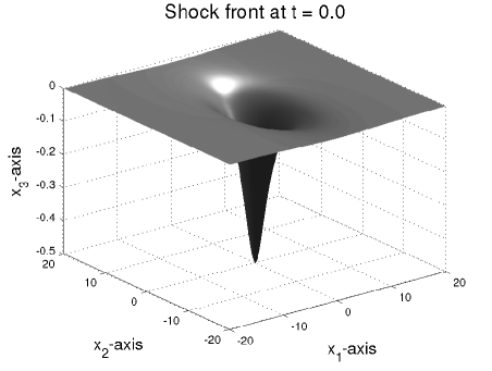
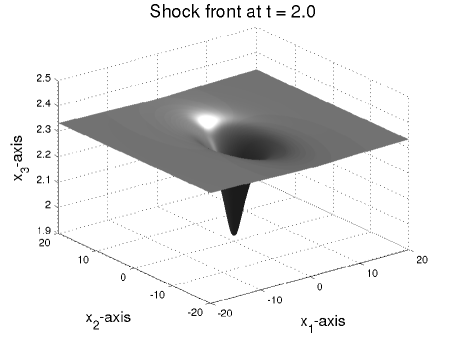
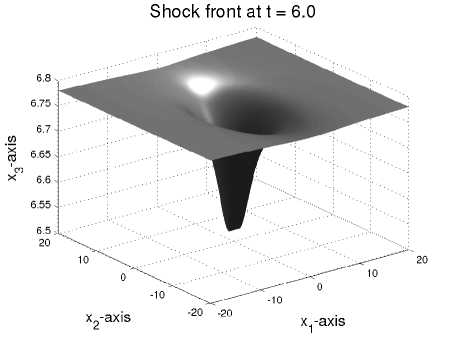
Figure 1. The successive positions of the shock front $\Omega_{t}$ with an initial smooth non-symmetric dip which is not axisymmetric.

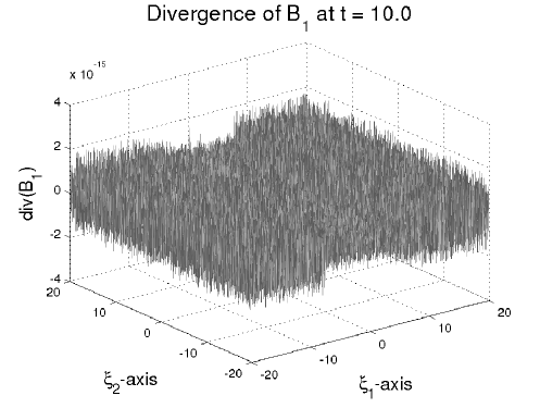
Figure 2. The discrete divergence of $\mathfrak{B}_{1}$ at $t=10.0$. The error is of the order of $10^{-15}$.

4.2. Corrugation Stability of a Shock Front and Interaction of Kink Lines

The corrugation stability of a front is defined as the stability of a planar front to perturbations. This means that the perturbations in the shape of a planar front ultimately disappear as time tends to infinity. The extensive numerical simulations by Monica and Prasad [18], using 2-D SRT, clearly show that a 2-D shock front is corrugation stable. From [18] we reproduce Figure 3, where continuous lines are successive positions of the 2-D initially sinusoidal shock front, the broken lines are the rays and dots are the kinks. The shock has become almost a straight line much before $t=40$. Similarly, the results of numerical experiments with 3-D WNLRT, reported in [2, 3], show that a 3-D nonlinear wavefront is also corrugation stable. The aim of this test case is to verify the corrugation stability of a 3-D shock front, evolving according to 3-D SRT, and describe the interaction of kink lines.

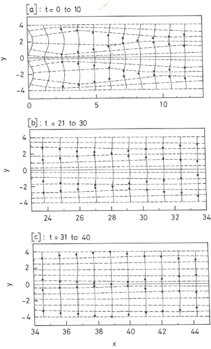
Figure 3. Successive positions of an initially sinusoidal shock front and rays from [18], plotted at $t=0,1,2,3,\ldots,40$. The initial shock front is $x=0.2-0.2\cos(\pi y/2)$ with $M_{0}=1.2$ and $\mathcal{V}_{0}=0.1$.

The corrugation stability is a result of the genuine nonlinearity in the characteristic fields corresponding to the two nonzero eigenvalues of the system (2.33). The shocks in the $(\xi_{1},\xi_{2},t)$-coordinates, which are mapped onto kinks, cause dissipation of the kinetic energy. Notice that the energy transport equation (2.31) of 3-D WNLRT is homogeneous, whereas the corresponding equation (2.23) of 3-D SRT has a source term. In the case of a nonlinear wavefront, the value of $m-1$ converges to the mean value of $m_{0}-1$. For a shock, when $\mathcal{V}>0$, the value of $M-1$ decreases to zero. This is typical of a plane shock in gas dynamics, which can also be seen from the 1-D model equation $u_{t}+(u^{2}/2)_{x}=0$; see [22]. Thus, the value of $M-1$, in addition to approaching a constant value, decays. The result is that the perturbations in the shape of the shock front not only disappear, leading to corrugation stability, but also the front velocity $M$ approaches the linear front velocity $M=1$. We refer the reader to [18] for a related discussion on the corrugation stability of 2-D shock fronts.

In order to verify the corrugation stability, we consider here the initial shock front $\Omega_{0}$ to be of a periodic shape in $x_{1}$- and $x_{2}$-directions

(4.3) $$\Omega_{0}\colon x_{3}=\kappa\left(2-\cos\left(\frac{\pi x_{1}}{a}\right)-\cos\left(\frac{\pi x_{2}}{b}\right)\right)$$

with the constants $\kappa=0.1,a=b=2$. In Figure 4 we give the plot of the initial shock front $\Omega_{0}$, which is a smooth pulse without any kink lines. The initial front $\Omega_{0}$ can be thought of modelling a smooth perturbation of a plane front. We prescribe a constant initial velocity $M_{0}=1.2$ everywhere on the front given in (4.3). Though the initial shock front is smooth, as the time evolves, a number of kink lines appear in each period. The process of interaction of these kink lines is a very interesting phenomena, which has not been described in [2]. In the following, we proceed to do it with a number of plots of the shock front at different instances.

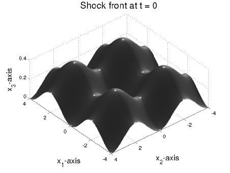
Figure 4. Initial shock front in the shape of a smooth periodic pulse.

In Figure 5 we give the surface plots of the shock front $\Omega_{t}$ at times $t=10,20,30,40,50,60$ in two periods in $x_{1}$ and $x_{2}$-directions. As mentioned above, the initial shock front is smooth, with no kink lines. The front $\Omega_{t}$ moves up in the $x_{3}$-direction and develops several kink lines. Four kink lines parallel to $x_{1}$-axis and four parallel to $x_{2}$-axis can be seen in the figures on the shock front at times $t\geq 10$. These kink lines are formed at a time before $t=10$, say about $t=2$. This can easily be observed from the Figure 6 showing the maximum and minimum values, $M_{\max}(t)$ and $M_{\min}(t)$, versus $t$, where $M_{\max}(t)$ and $M_{\min}(t)$ the maximum and minimum values of $M$ respectively taken over $(\xi_{1},\xi_{2})$ at any time $t$. We can observe a significant increase in the maximum value of $M$ near $t=2$ and it also jumps after the interaction of kink lines at later times.

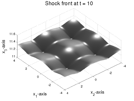
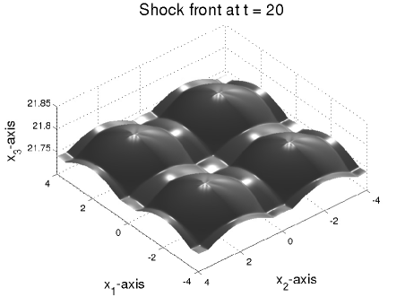
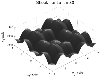
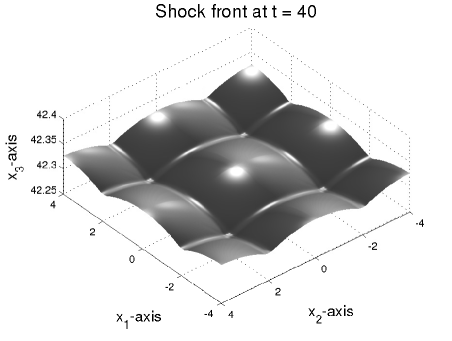
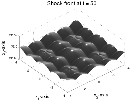
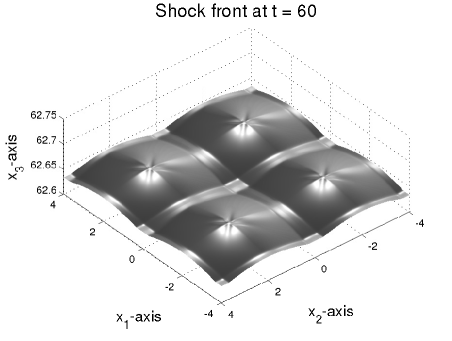
Figure 5. Shock front $\Omega_{t}$ starting initially in a periodic shape with $M_{0}=1.2$. The shock front develops a complex pattern of kinks and ultimately becomes planar.

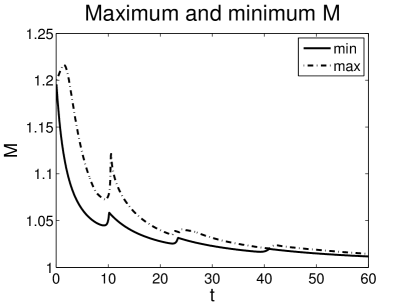
Figure 6. Variation of $M_{\max}(t)$ and $M_{\min}(t)$ with time from $t=0$ to $t=80$ for a periodic shock front $x_{3}=\kappa\left(2-\cos\left(\frac{\pi x_{1}}{a}\right)-\cos\left(\frac{\pi x_{2}}{b}\right)\right)$. The difference $M_{\max}(t)-M_{\min}(t)$ tends to zero as $t\to\infty$.

Due to symmetry, it is sufficient if we describe the motion of the kink lines parallel to the $x_{1}$-axis. Let us designate the part $-4\leq x_{1}\leq 0$ as the first period and $0\leq x_{1}\leq 4$ as second period. A pair of kink lines are seen in each period at $t=10$ near $x_{1}=-2$ and $x_{1}=2$, they are about to interact and produce another pair of kink lines. These newly formed kink lines move apart, cf. also the corresponding 2-D diagram in Figure 3. At $t=20$, one kink line from each of first and second periods have come quite near and are seen close to $x_{1}=0$. They interact, produce a new pair of kink lines and move apart as seen at $t=30$, where we find four distinct kink lines in $-4<x_{1}<4$. This process continues, two pairs of kink lines about to interact are seen near $x_{1}=-2$ and $x_{1}=2$ at $t=40$. There are four distinct kink lines also at $t=50$ and at $t=60$. The two kink lines near $x_{1}=0$ at $t=60$ are about to interact.

The interaction of kinks was first observed on a 2-D shock front experimentally in [29], cf. Figures 6(b) and (c) and numerically in [18], cf. Figure 3. We do observe the same phenomenon here, except that kinks are replaced by kink lines. A detailed theoretical analysis of this phenomenon on a 2-D nonlinear wavefront is presented in [6]. Interaction of kinks is a particular case of some interesting phenomena and in the following we briefly describe them; see also [6] for more details.

The equations of the 2-D KCL based WNLRT form a hyperbolic system of three conservation laws in $(\xi_{1},t)$-plane when $m>1$; see also (2.29)-(2.31) and (4.12). The system of conservation laws of 2-D WNLRT is not degenerate and there are no source terms. The characteristic fields corresponding to the two nonzero eigenvalues are genuinely nonlinear and corresponding to these fields we have four elementary wave solutions, which are shocks and centred rarefaction waves in $(\xi_{1},t)$-plane. The images of these elementary waves onto $(x_{1},x_{2})$-plane are called elementary shapes. As mentioned earlier, a shock is mapped onto an elementary shape kink in $(x_{1},x_{2})$-plane but a centred rarefaction wave is mapped on a continuous convex shape on the weakly nonlinear wavefront $\Omega_{t}$. Interaction of the elementary shapes in $(x_{1},x_{2})$-plane can be studied with the help of interactions of elementary waves in $(\xi_{1},t)$-plane. These interactions can be of finite or infinite duration in time. Two kinks of different characteristic family on $\Omega_{t}$ approach, interact and then produce another pair of kinks, which move apart.

For $M>1$, the KCL based 2-D SRT equations form a hyperbolic system of balance laws due to appearance of second terms in (2.27)-(2.28) which are source terms. However, the source terms, which affect the solution on larger space and time scales, do not have any effect on the interaction of two kinks on a shock front, which takes place instantaneously. They have only a small effect on the motion of kinks for a short time before and after the interaction. Thus, the nature of interaction of two kinks on a shock front as seen in Figure 3 is same as that of interaction of kinks on a nonlinear wavefront theoretically predicted in [6]. Interactions of two parallel kink lines on a 3-D shock front will be similar to that of the two kinks on a 2-D shock front. We clearly observe this in Figure 5 for the interaction of a pair of parallel kink lines. However, the interaction of oblique kink lines will be quite different about which we do not intent to make any comment.

Remark 4.2.

Comparing the shock fronts at different times in Figure 5, with the corresponding nonlinear wavefronts at the same time, we notice that the two fronts differ in their shapes. Let us compare the graphs of $M_{\max}(t)$ and $M_{\min}(t)$ in Figure 6 with those of $m_{\max}(t)$ and $m_{\min}(t)$ in Fig.11(a) of [2]. We find that $M_{\max}(t)$ and $M_{\min}(t)$ values on the shock front decay very rapidly compared to those on the nonlinear wavefront. As a result, the waves on the nonlinear wavefront move faster and the interaction of kink lines takes place more frequently. Graphs of $m_{\max}(t)$ and $m_{\min}(t)$ in Fig.10(a) of [2] oscillate quite fast. Since sudden increases in the values of $M_{\max}(t)$ and $M_{\min}(t)$ (and similarly those of $m_{\max}(t)$ and $m_{\min}(t)$) correspond to interactions of kink lines, we notice that kink lines on the nonlinear wavefront interact more frequently than those on a shock front.

4.3. A Shock Front Starting from an Axisymmetric Shape

Next we consider a shock front with an axisymmetric, oscillatory and radially decaying shape given by

(4.4) $$\Omega_{0}\colon x_{3}=\kappa\cos(\alpha r)e^{-\beta r},$$

where $r=\sqrt{x_{1}^{2}+x_{2}^{2}}$. The evolution of a nonlinear wavefront with this initial geometry has not been discussed in [2] and we present it here as yet another instance of corrugation stability. The initial shock front $\Omega_{0}$ models a smooth perturbation of a planar front such that the amplitude of the perturbation decays to zero as $r\to\infty$. The parameters in (4.4) are taken as $\kappa=0.05,\alpha=1.0,\beta=0.15$. The initial velocity has a constant value $M_{0}=1.2$ everywhere on the shock front.

In Figure 7 we give the surface plots of the initial shock front $\Omega_{0}$ and the shock front $\Omega_{t}$ at time $t=80$. It can be noted that the front $\Omega_{t}$ moves up in the $x_{3}$-direction. At $t=0$, there is an axisymmetric elevation near the origin $r=0$ and this central elevation decays fast. The smooth shape $\Omega_{0}$ at $t=0$ develops later a number of circular kink lines, however these kink lines have almost disappeared at $t=80$ since the height of the shock front has become quite small at this time. The elevations and depressions on the front diminish, leading to the reduction in height. We compute the maximum height $h(t)$ defined by

(4.5) $$h(t):={x_{3}}_{\max}(t)-{x_{3}}_{\min}(t),.$$

In Figure 8 we give the plot of $h$ versus $t$, which clearly shows that height reduces with time. The initial maximum height is $h(0)=0.08$, whereas at $t=80$ it is $h(80)=0.002917$, which corresponds to a $96.35\%$ reduction in the initial height. It is, therefore, very easy to see that the shock front tends to become planar, with its height decreasing to zero.

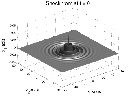
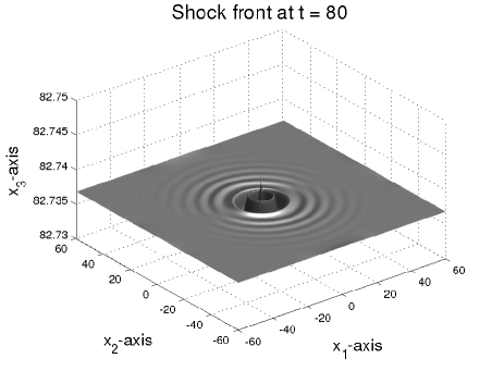
Figure 7. The evolution of a shock front $\Omega_{t}$ starting from a smooth pulse $x_{3}=0.05\cos(r)e^{-0.15r}$.

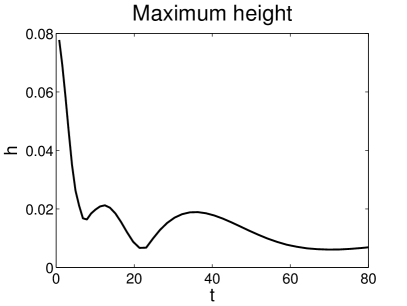
Figure 8. Time variation maximum height of the shock front given initially by $x_{3}=0.05\cos(r)e^{-0.15r}$.

Now we show that the normal velocity $M$ and the gradient $\mathcal{V}$ of the gas density at the shock tend to become constant as the computational time increases. As before, let us denote by $M_{\max}(t)$ and $M_{\min}(t)$, the maximum and minimum of $M$ taken over $(\xi_{1},\xi_{2})$ at any time $t$. In an analogous manner we define $\mathcal{V}_{\max}(t)$ and $\mathcal{V}_{\min}(t)$. In Figure 9(a)-(b) we plot the distribution of $M_{\max}(t),M_{\min}(t)$ and $M_{\max}(t)-M_{\min}(t)$ with respect to time from $t=0$ to $t=80$. It can be seen that both $M_{\max}(t)$ and $M_{\min}(t)$ decay to one with time and as a result, the difference $M_{\max}(t)-M_{\min}(t)$ tends to zero asymptotically. We have given the plot of $\mathcal{V}_{\max}(t),\mathcal{V}_{\min}(t)$ and $\mathcal{V}_{\max}(t)-\mathcal{V}_{\min}(t)$ in Figure 10(a)-(b). From the figure it is clear that both $\mathcal{V}_{\max}(t)$ and $\mathcal{V}_{\min}(t)$ approach zero as time increases.

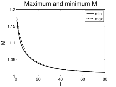
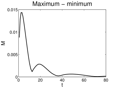
(a)	(b)

Figure 9. For an initial shock front $x_{3}=0.05\cos(r)e^{-0.15r}$ (a): variation of $M_{\max}(t)$ and $M_{\min}(t)$ with time from $t=0$ to $t=80$. (b): the difference $M_{\max}(t)-M_{\min}(t)$ tends to zero as $t\to\infty$.

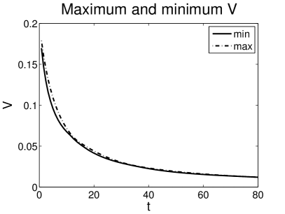
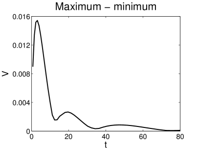
(a)	(b)

Figure 10. For an initial shock front $x_{3}=0.05\cos(r)e^{-0.15r}$ (a): variation of $\mathcal{V}_{\max}(t)$ and $\mathcal{V}_{\min}(t)$ with time from $t=0$ to $t=80$. (b): the difference $\mathcal{V}_{\max}(t)-\mathcal{V}_{\min}(t)$ tends to zero as $t\to\infty$.

4.4. Converging Shock Front Initially in the Shape of a Circular Cylinder

In this test problem we present the results of simulation of a cylindrically converging shock front. Even though this is basically a 2-D shock propagation problem, we intent to study it with our 3-D numerical method.

The initial geometry of the front is a portion of a circular cylinder of radius two units, i.e.

(4.6) $$\Omega_{0}\colon x_{1}^{2}+x_{2}^{2}=4,\ -\frac{\pi}{2}\leq x_{3}\leq\frac{\pi}{2}.$$

Initially, the ray coordinates $(\xi_{1},\xi_{2})$ are chosen as $\xi_{1}=x_{3}$ and $\xi_{2}=\theta$, where $\theta$ is the azimuthal angle. Therefore, the initial shock front $\Omega_{0}$, given in (4.6), can be expressed in a parametric form

(4.7) $$\Omega_{0}\colon x_{1}=2\cos\xi_{2},\ x_{2}=2\sin\xi_{2},\ x_{3}=\xi_{1},\ -\frac{\pi}{2}\leq\xi_{1}\leq\frac{\pi}{2},\ 0\leq\xi_{2}\leq 2\pi.$$

We have imposed periodic boundary conditions at $\xi_{2}=0$ and $\xi_{2}=2\pi$ and extrapolation boundary conditions at $\xi_{1}=\pm\pi/2$.

As a result of the particular choice of the ray coordinates $(\xi_{1},\xi_{2})$, the unit normal to $\Omega_{0}$ given by $\mbox{\boldmath$n$}_{0}=(-\cos\xi_{2},\sin\xi_{2},0)$, points inward and hence the front converges. If the initial velocity is given a uniform distribution on $\Omega_{0}$ as in the previous problems, the front $\Omega_{t}$ at any successive time $t$ will remain a circular cylinder with no interesting geometrical features. Our aim here is to study the stability of a focusing shock front to perturbations. Hence, the initial distribution of the normal velocity $M$ is given as a small perturbation of a constant value, i.e.

(4.8) $$M_{0}(\xi_{1},\xi_{2})=1.2+\alpha\cos(\nu\xi_{2})$$

with $\alpha=0.05$ and $\nu=8$.

In Figure 11 we give the plots of the initial shock front $\Omega_{0}$ and the shock front $\Omega_{t}$ at time $t=1.0$. The shock fronts are coloured using the variation of the normal velocity $M$, with the grayscale-bar on the right indicating the values of $M$. Note that the initial normal velocity $M_{0}$ has a periodic variation with a maximum value $1.25$ and a minimum value $1.05$, cf. (4.8). Those portions of the front where $M_{0}$ has maximum value moves inwards faster and it results in a distortion of the circular shape of $\Omega_{0}$. From the shock front at $t=1$ in Figure 11, it can be observed that sixteen fully developed vertical kink lines are formed on the shock front and kink lines have not yet interacted. Clearly, the number of plane sides and kink lines on $\Omega_{t}$ at various times will depend on the value of parameter $\nu$ in (4.8). The shock front assumes the shape of a polygonal cylinder and as time progresses the Mach stem-like surfaces on the shock front interacts, with the formation of new kink lines and this process repeats. It has to be remarked that our numerical results are well in accordance with the experimental results of [30], where the authors have reported that a converging shock front with a small perturbation assumes the shape of a polygon. This test problem, hence, gives another yet evidence for the efficacy of SRT to produce physically realistic geometrical features.

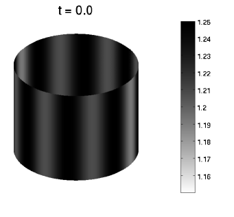
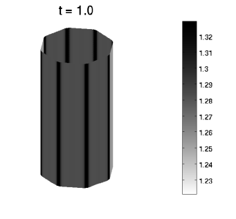
Figure 11. Cylindrically converging shock front. On the left the initial front and on the right the front at time $t=1.0$. The grayscale-bar on the right hand side indicates the intensity of the normal velocity $M$.

An examination of the shock front at $t=1.0$ in Figure 11 and the corresponding nonlinear wavefront in [2] shows that both the fronts have analogous geometry. We also refer the reader to [2] for more details on the transient geometries between the initial and final configurations and a quantification of the focusing process. Nevertheless, in order to point out the important difference in the case of a shock front, in Figure 12 we give the successive cross-sections (say by $x_{3}=0$ plane) of the shock fronts and the corresponding nonlinear wavefronts at times $t=0,0.1,0.2,\ldots,1.0$. Note that initially the normal speeds $m$ and $M$ of both the fronts have the same initial values. These speeds increase due to convergence of the fronts, however, in the case of a shock front there is also a decay in the shock speed due to interaction of the shock with the nonlinear wavefronts, cf. (also) the second term in (2.27). Therefore, as time increases, the shock front lags behind the nonlinear wavefront as seen in Figure 12.

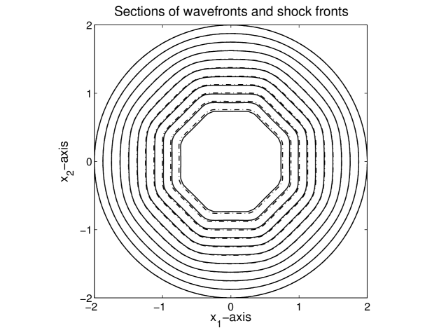
Figure 12. Cross-sections of the shock fronts (broken lines) and the nonlinear wavefront (continuous lines) at $t=0,0.1,0.2,\ldots,1.0$ by $x_{3}=0$ plane

4.5. Spherically Converging Shock Front

In this problem we consider the propagation of a spherically converging shock front. The initial geometry of the shock front is a sphere of radius two units. The ray coordinates are chosen to be $\xi_{1}=\pi-\phi$ and $\xi_{2}=\theta$, where $\theta$ is the azimuthal angle and $\phi$ is the polar angle. Therefore, the parametric representation of the initial shock front $\Omega_{0}$ is

(4.9) $$x_{1}=2\sin\xi_{1}\cos\xi_{2},\ x_{2}=2\sin\xi_{1}\sin\xi_{2},\ x_{3}=-2\cos\xi_{1}.$$

In order to avoid the singularities at $\phi=0$ and $\phi=\pi$, we remove these points. Therefore, our computational domain is $[\pi/15,14\pi/15]\times[0,2\pi]$. As in the previous problem, we choose the initial velocity distribution as a small perturbation of a constant value, i.e.

(4.10) $$M_{0}(\xi_{1},\xi_{2})=1.2+\alpha\cos(\nu_{1}\xi_{1})\cos(\nu_{2}\xi_{2})$$

with $\alpha=0.05,\nu_{1}=4,\nu_{2}=8$.

The 3-D plots of the initial shock front and the one at time $t=0.85$ are given in Figure 13. The shock fronts are coloured using the variation of the normal velocity $M$, with the grayscale-bar on the right indicating the values of $M$. It can be observed from the figure that as the front starts focusing, it develops several kink curves and its spherical shape gets distorted, with the formation of facets. The final shape of the shock front is almost a polyhedron.

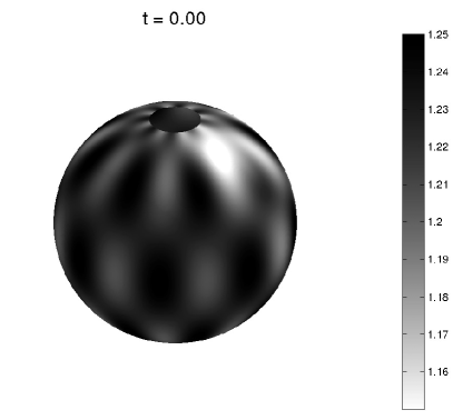
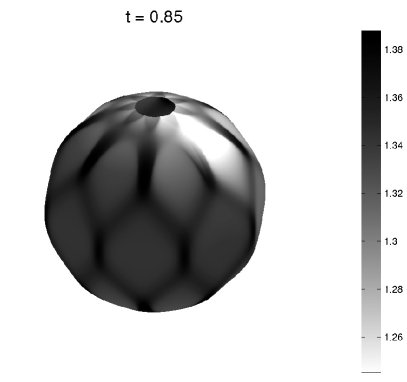
Figure 13. Spherically converging shock front at $t=0.85$. The grayscale bar on the right represents the distribution of $M$.

In this test problem also we have a observed qualitatively similar behaviour of a shock front and nonlinear wavefront. The major important difference is that the shock front slightly lags behind the nonlinear wave due to the effect on the shock of the flow behind the shock, as explained in the case of a cylindrically converging shock.

Remark 4.3.

It has to be emphasised that we can continue the computations further, however, the results would not be physically realistic as the weak shock ray theory breaks down for larger values of $M-1$.

Remark 4.4.

As in the case nonlinear wavefront in [2], we notice that cylindrically and spherically converging shocks take the polygonal and polyhedral shapes, respectively. These two shapes are stable configurations for the two cases. The stability here does not mean that once one of these configuration is formed, the shock front remains in this configuration for all time. It may change again into another such configuration.

4.6. Some More Comparison Between 3-D WNLRT and 3-D SRT

By comparing the results of numerical experiments presented above with those of 3-D WNLRT reported in ([2]), we infer that the geometrical shapes of nonlinear wavefronts and shock fronts are more or less qualitatively similar. However, looking at these shapes alone, it is not possible say much about the ultimate results as $t\to\infty$.

When the initial shape is periodic in $x_{1}$ and $x_{2}$ given by 4.3, we have examined the behaviour of a nonlinear wavefront in [2] and that of a shock front in subsection 4.2 for $t\to\infty$ and found that both are corrugationally stable. This means that both these fronts tend to become planar after a long time, which in turn shows that the mean curvature ${\it\Omega}$ approaches zero. Writing the differential form of (2.31) and letting ${\it\Omega}\to 0$, i.e. the mean curvature approaching zero yields

(4.11) $$m(\xi_{1},\xi_{2},t)\to\mathrm{const},\ \mbox{as}\ t\to\infty.$$

In order that the nonlinear wavefront be corrugation stable, this constant must be the same along all rays. It has been observed in [2] that even though the maximum and minimum of the front velocity $m$ of a nonlinear wavefront heavily oscillate about their initial values, they finally approach their initial mean values as $t\to\infty$. It is, therefore, very interesting to note that the numerical computation suggests the constant in (4.11) is $m_{0}$ for the case when $m_{0}$ is constant everywhere on the initial wavefront $\Omega_{0}$.

We now proceed to investigate the long term of behaviour of the perturbations on a 3-D corrugationally stable plane shock front. First, we note that the numerical results show that both $M_{\max}$ and $M_{\min}$ decrease to one with increasing time. Therefore, $M\to 1$ as $t\to\infty$, cf. subsections 4.2 and 4.3. The results also show that the gradient $\mathcal{V}$ of the pressure decays to zero as $t\to\infty$. Analogous results were reported also in the 2-D case in [18]. Thus, we can see a major difference in the decay of the shock amplitude from the corresponding results of 3-D WNLRT.

In order to do some more comparison of results for a nonlinear wavefront and shock front, we choose the initial geometry of the nonlinear wavefront and shock front to be an axisymmetric dip given in (4.2) with $\kappa=0.5,\alpha=\beta=1.5$. We take the same initial values of $M$ and $m$, both equal to 1.2. This choice is different from that in [18], where $\mu$ defined by (2.2) was chosen to be the same. Note that $M$ is given by (2.10), whereas for a nonlinear wavefront

(4.12) $$m:=1+\varepsilon\frac{\gamma+1}{2}\mu.$$

The computations are done with 3-D WNLRT and 3-D SRT up to a time $t=10$. A comparison of the results obtained is presented in Figure 14, where we have plotted the successive wavefronts and shock fronts in the section $x_{2}=0$ from $t=0$ to $t=10$ in a time step of $0.5$. In the figure, the solid lines represent the successive nonlinear wavefronts and dotted lines are the shock fronts. The figure clearly shows that from time $t=2.0$ onwards, the nonlinear wavefront overtakes the corresponding shock front. We also notice that the central portion of the nonlinear wavefront bulges out and the two kinks move apart faster than those on the shock front.

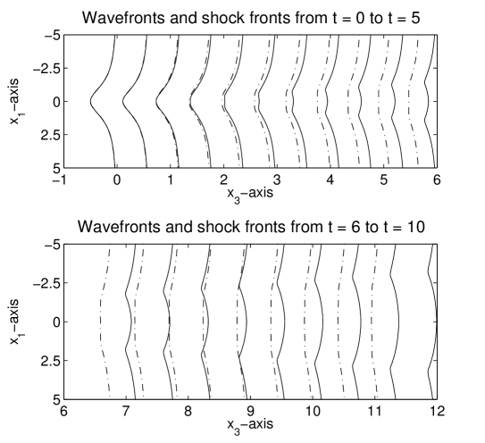
Figure 14. Comparison of the results by 3-D WNLRT and 3-D SRT. Figure on the top: from $t=0.0$ to $t=5.0$ and bottom: from $t=6.0$ to $t=10.0$. The solid lines represent successive positions of the nonlinear wavefront obtained by 3-D WNLRT and dotted lines are those of the shock front from 3-D SRT. The kinks can be noticed on both the fronts. The nonlinear wavefront overtakes the shock and its central portion bulges out so that the kinks on it are very prominent.

We also present in Figure 15 the graphs of the normal velocity $m$ of the nonlinear wavefront and $M$ of that of the shock front. In the figure we have plotted both $m$ and $M$ at times $0,2,4,6,8,10$ with the same constant initial values on the respective fronts. The Mach number at the centre of the fronts initially rises considerably in both the cases but it becomes constant on the central disc at time $t=4$ for the nonlinear wavefront. As the rays starts diverging from the bulged central portion, cf. Figure 15(a), we can see that $m$ reduces at the central portion from $t=6$ onwards. However, as seen in all previous cases with $\mathcal{V}_{0}>0$, the shock Mach number (and hence the shock amplitude) decreases with time on all parts of the shock front governed by 3-D SRT.

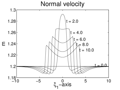
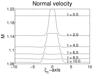
(a)	(b)

Figure 15. Comparison of the Mach number distribution on the fronts at times $0,2,4,6,8,10$ with the same amplitude distribution on the initial fronts. (a): results obtained by 3-D WNLRT. (b): those of 3-D SRT.

5. Concluding Remarks

Using the 3-D KCL based SRT we have successfully calculated the evolution of several shock surfaces, starting from a wide range of very interesting initial shapes. The proposed theory and numerical solution procedure correctly takes into account of the effect of the flow behind the shock, which is very important for weak shocks. It has been observed that the geometry, position and amplitude of a shock depends on its initial position, amplitude distribution and gradient of flow variables behind it. A comparison of the results with those of a weakly nonlinear wavefront shows that a weak shock front and a weakly nonlinear wavefront are topologically same.

With the aid of extensive numerical simulations, we have been able to verify the corrugational stability of a planar shock and have quantified the decay of small perturbations in the shape of a planar front. The simulation of cylindrically and spherically converging shock fronts shows that they assume polygonal and polyhedral shapes, receptively. These configurations appear to be stable in the sense that every such periodic distribution of $M$ on an initially cylindrical and spherical shock is likely to lead to polygonal and polyhedral shapes, which later on may get transformed to other similar shapes due to interaction of kink lines. However, our computations was not be continued further as the small amplitude assumption is violated because the value of $M$ increased too much due to radial convergence. Further calculation requires a new formulation of both WNLRT and SRT for the arbitrary amplitude case, along the lines of [23], and is a subject matter for future research.

In all the numerical simulations, particularly in long time computations, we have observed an interesting phenomenon of the persistence of kinks curves. As we have seen in all the cases considered by us, a kink curve may appear on an initially smooth shock front, but once it is formed it persists till it meets another kink curve. The persistence of a kink follows from the similar property of a shock in a genuinely nonlinear characteristic field; a shock, once formed cannot terminate at a finite distance in the $(\xi_{1},\xi_{2},t)$-space; see [22]. We further notice that interaction of a pair of kink curves (whether they correspond to the same characteristic field or different characteristic fields) always produces another pair of kink curves; see [6].

Appendix A Jacobian Matrices

A quasilinear form of the balance equations (2.33) of 3-D SRT can be written in a matrix form

(A.1) $$\tilde{A}V_{t}+\tilde{B}^{(1)}V_{\xi_{1}}+\tilde{B}^{(2)}V_{\xi_{2}}=\tilde{C},$$

where $V=(U_{1},U_{2},V_{1},V_{2},M,G_{1},G_{2},\mathcal{V})^{T}$. The Jacobian matrices $\tilde{A}=(\tilde{a}_{ij}),\tilde{B}^{(1)}=({\tilde{b}}^{(1)}_{ij})$ and $\tilde{B}^{(2)}=({\tilde{b}}^{(2)}_{ij})$ are of size $8\times 8$ and the vector $\tilde{C}$ belongs to $\mathbb{R}^{8}$. The nonzero elements of $\tilde{A},\tilde{B}^{(1)},\tilde{B}^{(2)}$ and $\tilde{C}$ are given below.

$${\tilde{a}}_{11}={\tilde{a}}_{22}=G_{1},\ {\tilde{a}}_{33}=G_{2},\ {\tilde{a}}_{44}=G_{2},\ {\tilde{a}}_{51}=-\frac{1}{U_{3}}G_{1}G_{2}N_{2}\cot\chi,\ {\tilde{a}}_{52}=\frac{1}{U_{3}}G_{1}G_{2}N_{1}\cot\chi,$$

$${\tilde{a}}_{53}=\frac{1}{V_{3}}G_{1}G_{2}N_{2}\cot\chi,\ {\tilde{a}}_{54}=-\frac{1}{V_{3}}G_{1}G_{2}N_{1}\cot\chi,\ {\tilde{a}}_{55}=\frac{2M}{M-1}G_{1}G_{2},\ {\tilde{a}}_{56}=G_{2},\ {\tilde{a}}_{57}=G_{1},$$

$${\tilde{a}}_{66}={\tilde{a}}_{77}=1,\ {\tilde{a}}_{81}=-\frac{1}{U_{3}}G_{1}G_{2}N_{2}\cot\chi,\ {\tilde{a}}_{82}=\frac{1}{U_{3}}G_{1}G_{2}N_{1}\cot\chi,\ {\tilde{a}}_{83}=\frac{1}{V_{3}}G_{1}G_{2}N_{2}\cot\chi,$$

$${\tilde{a}}_{84}=-\frac{1}{V_{3}}G_{1}G_{2}N_{1}\cot\chi,\ {\tilde{a}}_{85}=2G_{1}G_{2},\ {\tilde{a}}_{86}=G_{2},\ {\tilde{a}}_{87}=G_{1},\ {\tilde{a}}_{88}=\frac{2G_{1}G_{2}}{\mathcal{V}}$$

$${\tilde{b}}^{(1)}_{11}=-\frac{M}{U_{3}}(U_{1}U_{2}+N_{1}N_{2})\cot\chi,\ {\tilde{b}}^{(1)}_{12}=\frac{M}{U_{3}}(U^{2}_{1}+N^{2}_{1}-1)\cot\chi,$$

$${\tilde{b}}^{(1)}_{13}=\frac{M}{V_{3}\sin\chi}(U_{2}V_{1}+N_{1}N_{2}\cos\chi),\ {\tilde{b}}^{(1)}_{14}=-\frac{M}{V_{3}\sin\chi}(U_{1}V_{1}+(N^{2}_{1}-1)\cos\chi),\ {\tilde{b}}^{(1)}_{15}=-N_{1}.$$

$${\tilde{b}}^{(1)}_{21}=-\frac{M}{U_{3}}(U^{2}_{2}+N^{2}_{2}-1)\cot\chi,\ {\tilde{b}}^{(1)}_{22}=\frac{M}{U_{3}}(U_{1}U_{2}+N_{1}N_{2})\cot\chi,$$

$${\tilde{b}}^{(1)}_{23}=\frac{M}{V_{3}\sin\chi}(U_{2}V_{2}+(N_{2}^{2}-1)\cos\chi),\ {\tilde{b}}^{(1)}_{24}=-\frac{M}{V_{3}\sin\chi}(U_{1}V_{2}+N_{1}N_{2}\cos\chi),\ {\tilde{b}}^{(1)}_{25}=-N_{2}.$$

$${\tilde{b}}^{(1)}_{61}=-\frac{M}{U_{3}\sin\chi}(V_{2}-U_{2}\cos\chi),\ {\tilde{b}}^{(1)}_{62}=\frac{M}{U_{3}\sin\chi}(V_{1}-U_{1}\cos\chi).$$

$${\tilde{b}}^{(2)}_{31}=-\frac{M}{U_{3}\sin\chi}(U_{1}V_{2}+N_{1}N_{2}\cos\chi),\ {\tilde{b}}^{(2)}_{32}=\frac{M}{U_{3}\sin\chi}(U_{1}V_{1}+(N^{2}_{1}-1)\cos\chi),$$

$${\tilde{b}}^{(2)}_{33}=\frac{M}{V_{3}}(V_{1}V_{2}+N_{1}N_{2})\cot\chi,\ {\tilde{b}}^{(2)}_{34}=-\frac{M}{V_{3}}(V^{2}_{1}+N^{2}_{1}-1)\cot\chi,\ {\tilde{b}}^{(2)}_{35}=-N_{1}.$$

$${\tilde{b}}^{(2)}_{41}=-\frac{M}{U_{3}\sin\chi}(U_{2}V_{2}+(N^{2}_{2}-1)\cos\chi),\ {\tilde{b}}^{(2)}_{42}=\frac{M}{U_{3}\sin\chi}(U_{2}V_{1}+N_{1}N_{2}\cos\chi),$$

$${\tilde{b}}^{(2)}_{43}=\frac{M}{V_{3}}(V^{2}_{2}+N^{2}_{2}-1)\cot\chi,\ {\tilde{b}}^{(2)}_{44}=-\frac{M}{V_{3}}(V_{1}V_{2}+N_{1}N_{2})\cot\chi,\ {\tilde{b}}^{2}_{45}=-N_{2}.$$

$${\tilde{b}}^{(2)}_{73}=\frac{M}{V_{3}\sin\chi}(U_{2}-V_{2}\cos\chi),\ {\tilde{b}}^{(2)}_{74}=-\frac{M}{V_{3}\sin\chi}(U_{1}-V_{1}\cos\chi).$$

$$\tilde{c}_{7}=-\frac{2M}{M-1}G_{1}G_{2}\mathcal{V},\ \tilde{c}_{8}=-2MG_{1}G_{2}\mathcal{V}.$$

Appendix B Some Explanations of the KCL Based SRT

1. There are two parts in our method. The first part (purely geometrical) consists of KCL, in which the six jump relations imply conservation of distances in $x_{1},x_{2}$ and $x_{3}$ directions (and hence in any arbitrary direction in x-space) across a shock, see theorem 3.1 on page 297 of [4], also the section 3.3.3 of [22] for a detailed discussion.

The second part consists of the two closure relations (2.7)-(2.8) or (2.23) and (2.26), which are derived from the Euler equations of gas-dynamics. Out of these two closure relations, the first one explicitly represents conservation of energy along a shock ray. We note that the 4 jump relations of a 2-D shock (representing conservation of mass, momentum and energy) express all quantities behind the shock in terms of the unit normal $\bf N$ to the shock and a single unknown, say the Mach number $M$ of the shock. Time rate of change along a ray of $\bf N$ is a geometrical relation and is implied by KCL (see section 5, [4]) . Therefore, it is sufficient know the rate of change of $M$ along a shock ray. This is the basis of the derivation of the infinite system of equations by Grinfel’d [12] and Maslov [17]. Thus the two equations for $M$ and $\mathcal{V}$ along a shock ray in NTSD, implicitly take into account of conservation of mass and momentum also.

The geometrical conservation laws give the jump relations across a kink. The Euler equations, which are used to deduce the two compatibility conditions in conservation form, cannot account for the kink phenomenon. Initially, we had only the transport equation for $M$ along a shock ray in differential form [28]. Thus, we started with Euler equations. It was the need for capturing the kinks (geometrical singularities) on a shock that led to the formulation (or discovery) of 2-D KCL [19] in 1992 and 3-D KCL [11] in 1995.

2. At the end of the section 2 on page 5 we have stated ”For a discussion on the validity of NTSD and its application to 2-D problems we refer the reader to [7, 14, 18, 22]. It is interesting to note that the NTSD gives quite good results even for a shock of arbitrary strength, which has been verified for a 1-D piston problem in [16]. In addition, it has also been observed in [16] that the NTSD takes less than $0.5\%$ of the computational time needed by a typical finite difference method applied to the Euler equations.” Let me elaborate some of these below.

Before we found KCL, we had the NTSD in differential form and that is equivalent to KCL based shock ray theory for smooth shocks. While formulating the NTSD with a model equation, we showed a good agreement with exact solution [26] and a companion paper in the same journal. Ravindran, Sunder and Prasad also found good agreement in 1994 (see reference to this work in [14]). The first detailed attempt to verify and compare our method with other methods was done by Kevlahan [14]. Though he used the NTSD in differential form, he had a method to locate the kinks (see page 180 in [14]) and this method indeed gives the kinks location (see [22], page 126). Kevlahan cocludes ”The theory is tested against known analytical solutions for cylindrical and plane shocks, and against a full direct numerical simulation (DNS) of a shock propagating into a sinusoidal shear flow. The test against DNS shows that the present theory accurately predicts the evolution of a moderately weak shock front, including the formation of shock-shocks due to shock focusing. The theory is then applied to the focusing of an initially parabolic shock and he finds that the shock shapes (by this theory) agreed well with the experimental results”.

Since our theory is valid for a weak shock, we cannot compare with similarity solution of Guderley but, Kevlahan even compares a higher order theory of ours and finds remarkably good agreement.

A later reference [7] using 2-D KCL contains another extensive comparison of results with numerical solution of Euler equations.

3. The choice that the characteristic length $L$ is of the order of the distance over which 3-D SRT is valid, though it may look a bit vague but is an appropriate choice. A clear choice could have been the inverse of the mean curvature of the initial geometry of the shock. But due to appearance of the kinks, this information is lost in examples in subsection 4.2 and subsection 4.3 and solution is valid for almost infinite time. In the example in subsection 4.1 our result is calculated up to time $t=10$ and shock has moved approximately by a distance 11.08. However, we stop the computation at this stage as the value of $M$ increases beyond the validity of weak shock assumption. In the examples in subsection 4.4 and subsection 4.5, we could have taken $L$ to be the radius of the cylinder and that of the sphere respectively - these are of the order of the distance traveled by the shock. Computation in these cases were stopped because the value of $M-1$ became too large for the weak shock assumption to be valid.

References

- [1] A. M. Anile and G. Russo. Corrugation stability for plane relativistic shock waves. Phys. Fluids, 29:2847–2852, 1986.
- [2] K. R. Arun. A numerical scheme for three-dimensional front propagation and control of Jordan mode. SIAM J. Sci. Comput., 34:B148–B178, 2012.
- [3] K. R. Arun, M. Lukáčová-Medvid’ová, P. Prasad, and S. V. Raghurama Rao. An application of 3-D kinematical conservation laws: propagation of a three dimensional wavefront. SIAM J. Appl. Math., 70:2604–2626, 2010.
- [4] K. R. Arun and P. Prasad. 3-D kinematical conservation laws (KCL): evolution of a surface in -in particular propagation of a nonlinear wavefront. Wave Motion, 46:293–311, 2009.
- [5] K. R. Arun and P. Prasad. Eigenvalues of kinematical conservation laws (KCL) based 3-D weakly nonlinear ray theory (WNLRT). Appl. Math. comput., 217:2285–2288, 2010.
- [6] S. Baskar and P. Prasad. Riemann problem for kinematical conservation laws and geometrical features of nonlinear wavefronts. IMA J. Appl. Math., 69:391–420, 2004.
- [7] S. Baskar and P. Prasad. Propagation of curved shock fronts using shock ray theory and comparison with other theories. J. Fluid Mech., 523:171–198, 2005.
- [8] S. Baskar and P. Prasad. Formulation of the sonic boom problem by a maneuvering aerofoil as a one parameter family of cauchy problems. Proc. Indian Acad. Sci. Math. Sci., 116:97–119, 2006.
- [9] Y. Choquet-Bruhat. Ondes asymptotiques et approchées pour des systèmes d’équations aux dérivés partielles non linéaires. J. Math. Pures. Appl., 48:117–158, 1969.
- [10] C. R. Evans and J. F. Hawley. Simulation of magnetohydrodynamic flows-A constrained transport method. Astrophys. J., 332:659–677, 1988.
- [11] M. B. Giles, P. Prasad, and R. Ravindran. Conservation forms of equations of three dimensional front propagation. Technical report, Department of Mathematics, Indian Institute of Science, Bangalore, India, 1995.
- [12] M. A. Grinfel’d. Ray method for calculating the wavefront intensity in nonlinear elastic material. PMM J. Appl. Math. Mech., 42:958–977, 1978.
- [13] G.-S. Jiang and C.-W. Shu. Efficient implementation of weighted ENO schemes. J. Comput. Phys., 126:202–228, 1996.
- [14] N. K.-R. Kevlahan. The propagation of weak shocks in non-uniform flows. J. Fluid Mech., 327:161–197, 1996.
- [15] A. Kurganov and E. Tadmor. New high-resolution central schemes for nonlinear conservation laws and convection-diffusion equations. J. Comput. Phys., 160:241–282, 2000.
- [16] M. P. Lazarev, P. Prasad, and S. K. Sing. An approximate solution of one-dimensional piston problem. Z. Angew. Math. Phys., 46:752–771, 1995.
- [17] V. P. Maslov. Propagation of shock waves in an isentropic non-viscous gas. J. Sov. Math., 13:119–163, 1980.
- [18] A. Monica and P. Prasad. Propagation of a curved weak shock. J. Fluid Mech., 434:119–151, 2001.
- [19] K. W. Morton, P. Prasad, and R. Ravindran. Conservation forms of nonlinear ray equations. Technical report, Department of Mathematics, Indian Institute of Science, Bangalore, India, 1992.
- [20] P. Prasad. Approximation of perturbation equations of a quasilinear hyperbolic system in the neighbourhood of a bicharacteristic. J. Math. Anal. Appl., 50:470–482, 1975.
- [21] P. Prasad. Kinematics of a multi-dimensional shock of arbitrary strength in an ideal gas. Acta Mech., 45:163–176, 1982.
- [22] P. Prasad. Nonlinear hyperbolic waves in multi-dimensions, volume 121 of Chapman & Hall/CRC Monographs and Surveys in Pure and Applied Mathematics. Chapman & Hall/CRC, Boca Raton, FL, 2001.
- [23] P. Prasad and D. F. Parker. A shock ray theory for propagation of a curved shock of arbitrary strength. Technical report, Department of Mathematics, Indian Institute of Science, Bangalore, India, 1994.
- [24] P. Prasad and K. Sangeeta. Numerical simulation of converging nonlinear wavefronts. J. Fluid Mech., 385:1–20, 1999.
- [25] T. M. Ramanathan. Huygen’s method of construction of weakly nonlinear wavefronts and shockfronts with application to hyperbolic caustics. PhD thesis, Indian Institute of Science, Bangalore, India, 1985.
- [26] R. Ravindran and P. Prasad. A new theory of shock dynamics part 1: analytical considerations. Appl. Math. Lett., 3:77–81, 1990.
- [27] C.-W. Shu. Total-variation-diminishing time discretizations. SIAM J. Sci. Stat. Comput., 9:1073–1084, 1988.
- [28] R. Srinivasan and P. Prasad. On the propagation of a multidimensional shock of arbitrary strength. Proc. Indian Acad. Sci. Math. Sci., 94:27–42, 1985.
- [29] B. Sturtevant and V. A. Kulkarny. The focusing of weak shock waves. J. Fluid Mech., 73:651–671, 1976.
- [30] K. Takayama, H. Kleine, and H. Grönig. An experimental investigation of the stability of converging cylindrical shock waves in air. Exp. Fluids, 5:315–322, 1987.
- [31] G. B. Whitham. Linear and nonlinear waves. Wiley-Interscience [John Wiley & Sons], New York, 1974. Pure and Applied Mathematics.