Real-time Semantic Segmentation of Crop and Weed for Precision Agriculture Robots Leveraging Background Knowledge in CNNs

Abstract

Precision farming robots, which target to reduce the amount of herbicides that need to be brought out in the fields, must have the ability to identify crops and weeds in real time to trigger weeding actions. In this paper, we address the problem of CNN-based semantic segmentation of crop fields separating sugar beet plants, weeds, and background solely based on RGB data. We propose a CNN that exploits existing vegetation indexes and provides a classification in real time. Furthermore, it can be effectively re-trained to so far unseen fields with a comparably small amount of training data. We implemented and thoroughly evaluated our system on a real agricultural robot operating in different fields in Germany and Switzerland. The results show that our system generalizes well, can operate at around 20 Hz, and is suitable for online operation in the fields.

I Introduction

Herbicides and other agrochemicals are frequently used in crop production but can have several side-effects on our environment. Thus, one big challenge for sustainable approaches to agriculture is to reduce the amount of agrochemicals that needs to be brought to the fields. Conventional weed control systems treat the whole field uniformly with the same dose of herbicide. Novel, perception-controlled weeding systems offer the potential to perform a treatment on a per-plant level, for example by selective spraying or mechanical weed control. This, however, requires a plant classification system that can analyze image data recorded in the field in real time and labels individual plants as crop or weed.

In this paper, we address the problem of classifying standard RGB images recorded in the crop fields and identify the weed plants, roughly at the framerate of the camera. This information can in turn be used to perform automatic and targeted weed control or to monitor fields and provide a status report to the farmer without human interaction. There exists several approaches to vision-based crop-weed classification. A large number of approaches, especially those that yield a high classification performance, do not only rely on RGB data but furthermore require additional spectral cues such as near infra-red information. Often, these techniques also rely on a pre-segmentation of the vegetation as well as on a large set of hand-crafted features. In this paper, we target RGB-only crop-weed classification without pre-segmentation and are especially interested in computational efficiency for real-time operation on a mobile robot, see Fig. 1 for an illustration.

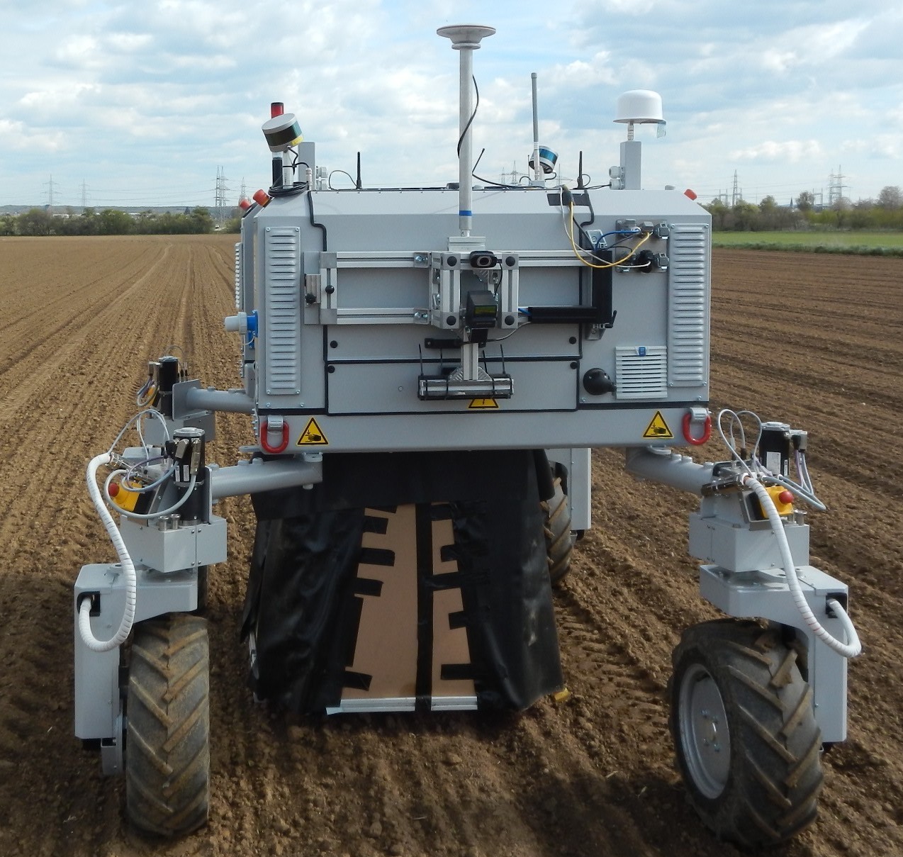
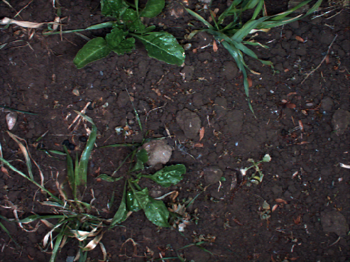
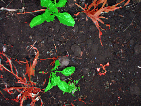
Figure 1: Left: Bonirob system, used for data acquisition and field deployment. Right: RGB image (top) captured during field test and our corresponding classification result with crops colored green and weeds colored red (bottom).

The main contribution of this work is a new approach to crop-weed classification using RGB data that relies on convolutional neural networks (CNNs). We aim at feeding additional, task-relevant background knowledge to the network in order to speed up training and to better generalize to new crop fields.

We achieve that by augmenting the input to the CNN with additional channels that have previously been used when designing hand-crafted features for classification [11] and that provide relevant information for the classification process. Our approach yields a pixel-wise semantic segmentation of the image data and can, given the structure of our network, be computed at near the frame-rate of a typical camera.

In sum, we make three key claims, which are the following: Our approach is able to (i) accurately perform pixel-wise semantic segmentation of crops, weeds, and soil, properly dealing with heavily overlapping objects and targeting a large variety of growth stages, without relying on expensive near infra-red information; (ii) act as a robust feature extractor that generalizes well to lighting, soil, and weather conditions not seen in the training set, requiring little data to adapt to the new environment; (iii) work in real-time on a regular GPU such that operation at near the frame-rate of a regular camera becomes possible.

II Related Work

In the context of crop classification, several supervised learning algorithms have been proposed in the past few years [7, 10, 11, 13, 15, 16, 19]. McCool et al. [13] address the crop and weed segmentation problem by using an ensemble of small CNNs compressed from a more complex pretrained model and report an accuracy of nearly 94%. Haug et al. [7] propose a method to distinguish carrot plants and weeds in RGB and near infra-red (NIR) images. They obtain an average accuracy of 94% on an evaluation dataset of 70 images. Mortensen et al. [16] apply a deep CNN for classifying different types of crops to estimate their amounts of biomass. They use RGB images of field plots captured at $3$ m above ground and report an overall accuracy of 80% evaluated on a per-pixel basis. Potena et al. [19] present a multi-step visual system based on RGB+NIR imagery for crop and weed classification using two different CNN architectures. A shallow network performs the vegetation detection and then a deeper network further distinguishes the detected vegetation into crops and weeds. They perform a pixel-wise classification followed by a voting scheme to obtain predictions for connected components in the vegetation mask. They report an average precision of $98$% in case the visual appearance has not changed between training and testing phase.

In our previous works [10, 11], we presented a vision-based classification system based on RGB+NIR images for sugar beets and weeds that relies on NDVI-based pre-segmentation of the vegetation. The approach combines appearance and geometric properties using a random forest classifier and obtains classification accuracies of up to 96% on pixel level. The works, however, also show that the performance decreases to an unsuitable level for weed control applications when the appearance of the plants changes substantially. In a second previous work [15], we presented a 2-step approach that pre-segments vegetation objects by using the NDVI index and afterwards uses a CNN classifier on the segmented objects to distinguish them into crops and weeds. We show that we can obtain state-of-the-art object-wise results in the order of 97% precision, but only for early grow stages, since the approach is not able to deal with overlapping plants due to the pre-segmentation step.

Lottes et al. [12] address the generalization problem by using the crop arrangement information, for example from seeding, as prior and exploit a semi-supervised random forest-based approach that combines this geometric information with a visual classifier to quickly adapt to new fields. Hall et al. [5] also address the issue of changing feature distributions. They evaluate different features for leaf classification by simulating real-world conditions using basic data augmentation techniques. They compare the obtained performance by selectively using different handcrafted and CNN features and conclude that CNN features can support the robustness and generality of a classifier.

In this paper, we also explore a solution to this problem using a CNN-based feature extractor and classifier for RGB images that uses no geometric prior, and generalizes well to different soil, weather, and illumination conditions. To achieve this, we use a combination of end-to-end efficient semantic segmentation networks and several vegetation indices and preprocessing mappings to the RGB images.

A further challenge for these supervised classification approaches is the necessary amount of labeled data required for retraining to adapt to a new field. Some approaches have been investigated to address to this problem such as [3, 20, 22]. Wendel and Underwood [22] address this issue by proposing a method for training data generation. They use a multi-spectral line scanner mounted on a field robot and perform a vegetation segmentation followed by a crop-row detection. Subsequently, they assign the label crop for the pixels corresponding to the crop row and the remaining ones as weed. Rainville et al. [20] propose a vision-based method to learn a probability distributions of morphological features based on a previously computed crop row. Di Cicco et al. [3] try to minimize the labeling effort by constructing synthetic datasets using a physical model of a sugar beet leaf. Unlike most of these approaches, our purely visual approach relies solely on RGB images and can be applied to fields where there is no crop row structure.

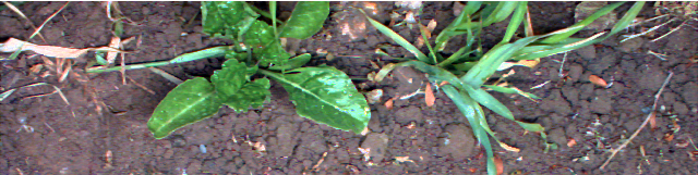
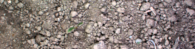
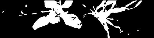
Figure 2: Example image of dataset A (left column) and dataset B (right column). Top row: RGB image. Middle row: Vegetation mask obtained by applying a global threshold learned by Otsu’s method, which fails for underrepresented vegetation. Bottom row: Vegetation detected by adaptive thresholding, which oversegments big plants. Failure cases are depicted in red.

In addition to the crop weed classification, several approaches have been developed for vision-based vegetation detection by using RGB as well as multispectral images, e.g., [4, 6, 11, 21]. Often, popular vegetation indices such as the Normalized Difference Vegetation Index (NDVI) or the Excess Green Index (ExG) are used to separate the vegetation from the background by applying threshold-based approaches. We see a major problem with these kind of approaches in terms of the transferability to other fields, i.e. when the underlying distribution of the indices changes due to different soil types, growth stages, illumination, and weather conditions. Fig. 2 visually illustrates frequent failure cases: First, a global threshold, here estimated by Otsu’s method, does not properly separate the vegetation if the plants are in a small growth stage, i.e. when the vegetation is underrepresented. This problem can be solved with adaptive thresholding, by tuning the kernel size and a local threshold for small plants. Second, the adaptive method fails, separating components that should be connected, when using the tuned hyperparameters in another dataset where the growth stage and field condition have changed. Thus, we argue that a learning approach that eliminates this pre-segmentation and solves segmentation and classification jointly is needed. As this paper illustrates, such strategy enables us to learn a semantic segmentation which generalizes well over several growth stages as well as field conditions.

III Approach

The main goal of our work is to allow agricultural robots to accurately distinguish weeds from value crops and soil in order to enable intelligent weed control in real time. We propose a purely visual pixel-wise classifier based on an end-to-end semantic segmentation CNN that we designed with accuracy, time and hardware efficiency as well as generalization in mind.

Our classification pipeline can be seen as being separated in two main steps: First, we compute different vegetation indices and alternate representations that are commonly used in plant classification and support the CNN with that information as additional inputs. This turns out to be specifically useful as the amount of labeled training data for agriculture fields is limited. Second, we employ a self-designed semantic segmentation network to provide a per-pixel semantic labeling of the input data. The following two subsections discuss these two steps of the pipeline in detail.

III-A Input Representations

In general, deep learning approaches make as little assumptions as possible about the underlying data distribution and let the optimizer decide how to adjust the parameters of the network by feeding it with enormous amounts of training data. Therefore, most approaches using convolutional neural networks make no modifications to the input data and feed the raw RGB images to the networks.

This means that if we want a deep network to accurately recognize plants and weeds in different fields, we need to train it with a large amount of data from a wide variety of fields, lighting and weather conditions, growth stages, and soil types. Unfortunately, this comes at a high cost and we therefore propose to make assumptions about the inputs in order to generalize better given the limited training data.

To alleviate this problem, we provide additional vegetation indexes that have been successfully used for the plant classification task and that can be derived from RGB data. In detail, we calculate four different vegetation indices which are often used for the vegetation segmentation, see [14, 18]: Excess Green (ExG), Excess Red (ExR), Color Index of Vegetation Extraction (CIVE), and Normalized Difference Index (NDI). These indices share the property that they are less sensitive to changes in the mentioned field conditions and therefore can aid the classification task. They are computed straightforwardly as:

$$\mathcal{I}_{\text{ExG}} =2\,\mathcal{I}_{\text{G}}-\mathcal{I}_{\text{R}}-\mathcal{I}_{\text{B}}$$ (1)

$$\mathcal{I}_{\text{ExR}} =1.4\,\mathcal{I}_{\text{R}}-\mathcal{I}_{\text{G}}$$ (2)

$$\mathcal{I}_{\text{CIVE}} =0.881\,\mathcal{I}_{\text{G}}-0.441\,\mathcal{I}_{\text{R}}-0.385\,\mathcal{I}_{\text{B}}-18.78745$$ (3)

$$\mathcal{I}_{\text{NDI}} =\frac{\mathcal{I}_{\text{G}}-\mathcal{I}_{\text{R}}}{\mathcal{I}_{\text{G}}+\mathcal{I}_{\text{R}}}$$ (4)

Along with these four additional cues, we use (i) further representations of the raw input such as the HSV color space and (ii) operators on the indices such as the Sobel derivatives, the Laplacian, and the Canny edge detector. All these representations are concatenated to the channel-wise normalized input RGB image and build the input volume which is fed into the convolutional network. In sum, we use the $14$ channels listed in Tab. I, and Fig. 3 illustrates how some of these representations look like. We show in our experiments that deploying these extra representations to the raw inputs helps not only to learn weight parameters which lead to a better generalization property of the network, but also obtain a better performance for separating the vegetation, i.e. crops and weeds, from soil, and speed up the convergence of the training process.

$\mathcal{I}_{\text{RGB}}$	$\mathcal{I}_{\text{ExG}}$	$\mathcal{I}_{\text{ExR}}$
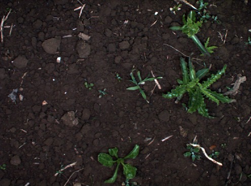
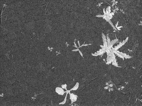
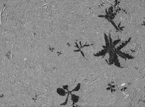
$\mathcal{I}_{\text{HUE}}$	$\mathcal{I}_{\text{EDGES}}$	$\nabla_{y}\mathcal{I}_{\text{ExG}}$

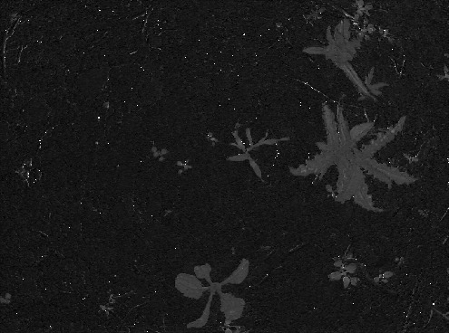
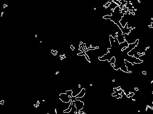
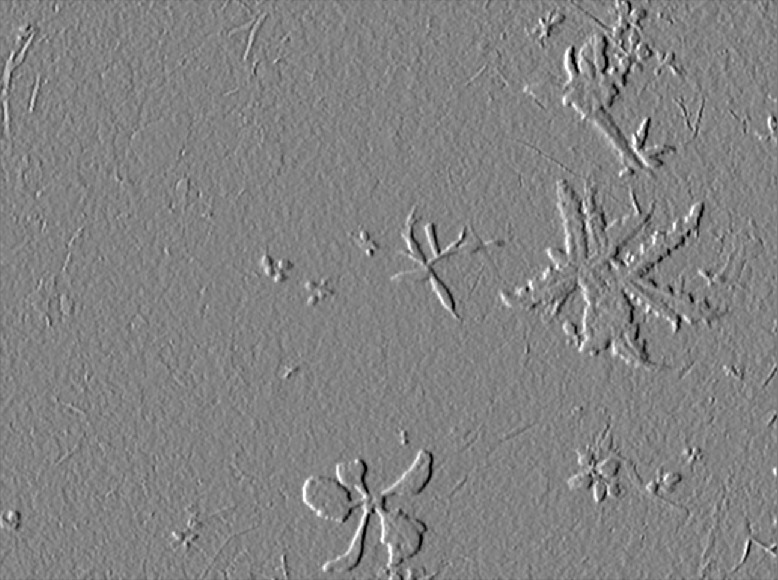
Figure 3: Illustration of some of the used alternate representations.

TABLE I: Indices and representations used as input by our CNN

Input channels for our CNN
$\mathcal{I}_{\text{1}}$	$\mathcal{I}_{\text{R}}$
$\mathcal{I}_{\text{2}}$	$\mathcal{I}_{\text{G}}$
$\mathcal{I}_{\text{3}}$	$\mathcal{I}_{\text{B}}$
$\mathcal{I}_{\text{4}}$	$\mathcal{I}_{\text{ExG}}$
$\mathcal{I}_{\text{5}}$	$\mathcal{I}_{\text{ExR}}$
$\mathcal{I}_{\text{6}}$	$\mathcal{I}_{\text{CIVE}}$
$\mathcal{I}_{\text{7}}$	$\mathcal{I}_{\text{NDI}}$
$\mathcal{I}_{\text{8}}$	$\mathcal{I}_{\text{HUE}}$ (from HSV colorspace)
$\mathcal{I}_{\text{9}}$	$\mathcal{I}_{\text{SAT}}$ (from HSV colorspace)
$\mathcal{I}_{\text{10}}$	$\mathcal{I}_{\text{VAL}}$ (from HSV colorspace)
$\mathcal{I}_{\text{11}}$	$\nabla_{x}\mathcal{I}_{\text{ExG}}$ (Sobel in x direction on $\mathcal{I}_{\text{ExG}}$)
$\mathcal{I}_{\text{12}}$	$\nabla_{y}\mathcal{I}_{\text{ExG}}$ (Sobel in y direction on $\mathcal{I}_{\text{ExG}}$)
$\mathcal{I}_{\text{13}}$	$\nabla^{2}\mathcal{I}_{\text{ExG}}$ (Laplacian on $\mathcal{I}_{\text{ExG}}$)
$\mathcal{I}_{\text{14}}$	$\mathcal{I}_{\text{EDGES}}$ (Canny Edge Detector on $\mathcal{I}_{\text{ExG}}$)

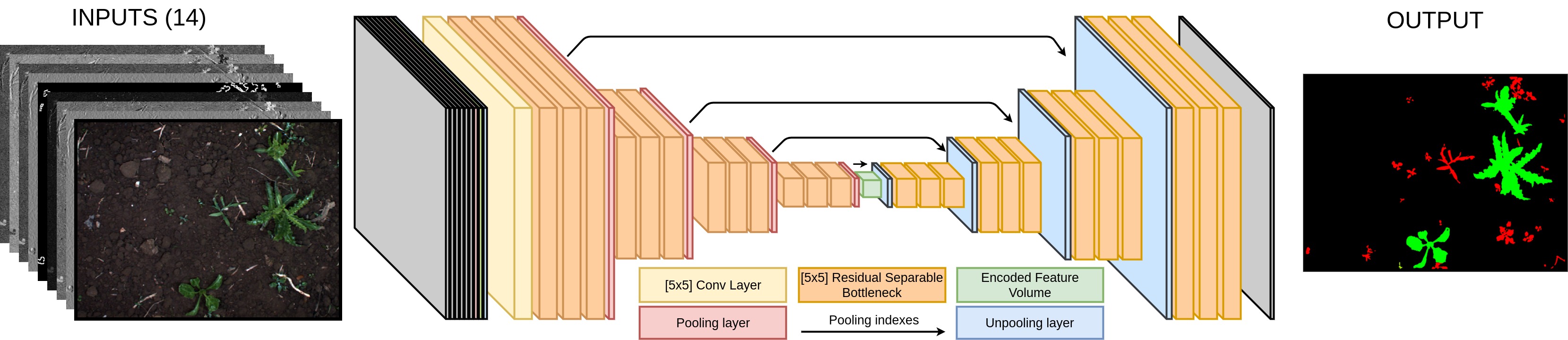
Figure 4: Detailed encoder-decoder architecture used for the pixel-wise semantic segmentation. Best viewed in color.

III-B Network Architecture

Semantic segmentation is a memory and computationally expensive task. State-of-the-art algorithms for multi-class pixel-wise classification use CNNs that have tens of millions of parameters and therefore need massive amounts of labeled data for training. Another problem with these networks is the fact that they often cannot be run fast enough for our application. The current state-of-the-art CNN for this task, Mask R-CNN [8], processes around 2 images per second, whereas we target on a classification rate of at least $10\,$\mathrm{H}\mathrm{z}$$.

Since our specific task of crop vs. weed classification has a much narrower target space compared to the general architectures designed for $1000$+ classes, we can design an architecture which meets the targeted speed and efficiency. We propose an end-to-end encoder-decoder semantic segmentation network, see Fig. 4, that can accurately perform the pixel-wise prediction task while running at $20\text{+}\,$\mathrm{H}\mathrm{z}$$, can be trained end-to-end with a moderate size training dataset, and has less than $30{,}000$ parameters. We design the architecture taking some design cues from Segnet [1] and Enet [17] into account and adapt them to the task at hand. Our network is based on the following building blocks:

Input: We use the representation volume described in Tab. I as the input to our network. Before it is passed to the first convolutional layer, we perform a resizing to $512\times 384$ pixels and a channel-wise contrast normalization.

Convolutional Layer: We define our convolutional layers as a composite function of a convolution followed by a batch normalization and use the rectified linear unit (ReLU) for the non-linearity. The batch normalization operation prevents an internal covariate shift and allows for higher learning rates and better generalization capabilities. The ReLU is computationally efficient and suitable for training deep networks. All convolutional layers use zero padding to avoid washing out edge information.

Residual Separable Bottleneck: To achieve a faster processing time while keeping the receptive field, we propose to use the principal building block for our network, which is built upon the ideas of (i) residual connections, (ii) bottlenecks, and (iii) separating the convolutional operations.

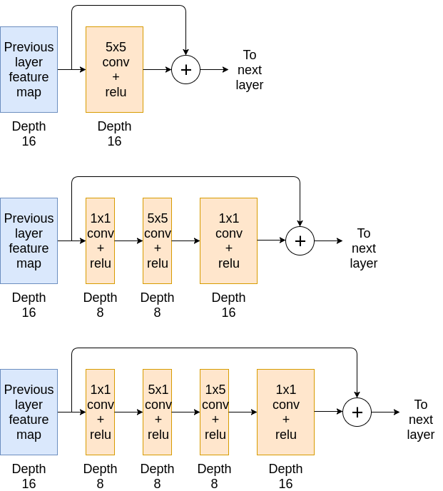
Figure 5: Building the residual block to replace a $[5\times 5]$ layer.

Fig. 5 illustrates the evolution from a conventional $[5\times 5]$ convolutional layer to a residual separable bottleneck. The top row of Fig. 5 shows the addition of a residual connection, which adds the input of the convolution to its result. The addition of this residual connection helps with the degradation problem that appears when training very deep networks which makes them obtain a higher training error than their shallower counterparts [9].

The middle row of Fig. 5 adds $[1\times 1]$ convolutions that reduce the depth of the input volume so that the expensive $[5\times 5]$ operation does not need to run in the whole depth. For this, we use $8\times[1\times 1]$ kernels, which halve the depth of the input volume, and $16\times[1\times 1]$ kernels to expand the result, which needs to match the depth of the input in order to be added to it. This reduces the amount of calculations per operation of the kernel from $6{,}400$ FLOPs to $1{,}856$ FLOPs.

Finally, the bottom row of Fig. 5 shows the separation of each $[5\times 5]$ convolution into a $[5\times 1]$ convolution followed by a $[1\times 5]$ convolution. This further reduces the operations of running the module in a $[5\times 5]$ window from $1{,}856$ FLOPs to $896$ FLOPs.

These design choices also decrease the number of parameters for the equivalent layer to the $[5\times 5]$ convolution with 16 kernels from $6{,}400$ to $896$ parameters.

Unpooling with Shared Indexes: The unpooling operations in the decoder are performed sharing the pooling indexes of the symmetrical pooling operation in the encoder part of the network. This allows the network to maintain the information about the spatial positions of the maximum activations on the encoder part without the need for transposed convolutions, which are comparably expensive to execute. Therefore, after each unpooling operation, we obtain a sparse feature map, which the subsequent convolutional layers learn how to densify. All pooling layers are $[2\times 2]$ with stride $2$.

Output: The last layer is a linear operation followed by a softmax activation predicting a pseudo-probability vector of length $3$ per pixel, where each element represents the probability of the pixel belonging to the class background, weed, or crop.

We use these building blocks to create the network depicted in Fig. 4, which consists of an encoder-decoder architecture. The encoder part has $13\times[5\times 5]$ convolutional layers containing $16$ kernels each and $4$ pooling layers that reduce the input representation into a small code feature volume. This is followed by a decoder with $12$ convolutional layers containing $16$ kernels each and $4$ unpooling layers that upsample this code into a semantic map of the same size of the input. The design of the architecture is inspired by Segnet’s design simplicity, but in order to make it smaller, easier to train, and more efficient, we replace $24$ of the $25$ convolutional layers by our proposed residual separable convolutional bottlenecks. The $5\times 5$ receptive fields of the convolutional layers, along with the pooling layers add up to an equivalent receptive field in the input image plane of $200\times 200$ pixels. This is sufficient for our application, since it is a bigger window than the biggest plant we expect in our data. The proposed number of layers, kernels per layer, and reduction factor for each bottleneck module was chosen by training several networks with different configurations, and reducing its size until we reached the smallest configuration that did not result in a considerable performance decrease.

IV Experimental Evaluation

TABLE II: Dataset Information

	Bonn	Zurich	Stuttgart
# images	10,036	2,577	2,584
# crops	27,652	3,983	10,045
crop pixels	1.7%	0.4%	1.5%
# weeds	65,132	14,820	7,026
weed pixels	0.7%	0.1%	0.7%

The experiments are designed to show the accuracy and efficiency of our method and to support the claims made in the introduction that our classifier is able to perform accurate pixel-wise classification of value crops and weeds, generalize well, and run in real-time.

We implemented the whole approach presented in this paper relying on the Google TensorFlow library, and OpenCV to compute alternate representations of the inputs. We tested our results using a Bosch Deepfield Robotics BoniRob UGV.

IV-A Training and Testing Data

To evaluate the performance of the network, we use three different datasets captured in Bonn, Germany; Stuttgart, Germany; and Zurich, Switzerland, see Tab. II. Part of the data from Bonn is publicly available [2]. All datasets contain plants and weeds in all growth stages, with different soil, weather, and illumination conditions. Fig. 6 illustrates the variance of the mentioned conditions for each dataset. The visual data was recorded with the 4-channel RGB+NIR camera JAI AD-130 GE mounted in nadir view. For our approach, we use solely the RGB channels because we aim to perform well with an off-the-shelf RGB camera, but the additional NIR information allows us to compare the performance with an approach that exploits the additional NIR information.

To show the generalization capabilities of the pipeline, we train our network using only images from Bonn, captured over the course of one month, and containing images of several growth stages. We separate the dataset in 70%-15%-15% for training, validation, and testing, and we report our results only in the latter 15% held out testing portion, as well as the whole of the two other datasets from Zurich and Stuttgart, some even recorded in different years.

We train the network using the 70% part of the Bonn dataset extracted for that purpose and perturb the input data by performing random rotations, scalings, shears and stretches. We use Stochastic Gradient Descent with a batch size of 15 for each step, which is the maximum we can fit in a single GPU. Furthermore, we use a weighted cross-entropy loss, to handle the imbalanced number of pixels of each class, due to the soil dominance, and the Adam optimizer for the calculation of the gradient steps. Training for 200 epochs takes roughly 48 hours on an NVIDIA GTX1080Ti.

To show the effect in performance obtained by the extra channels, we train three networks using different types of inputs: one based solely on RGB images, another one based on RGB and extra representations, and finally the reference baseline network using RGB+NIR image data.

Bonn	Zurich	Stuttgart

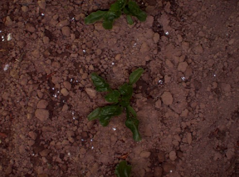
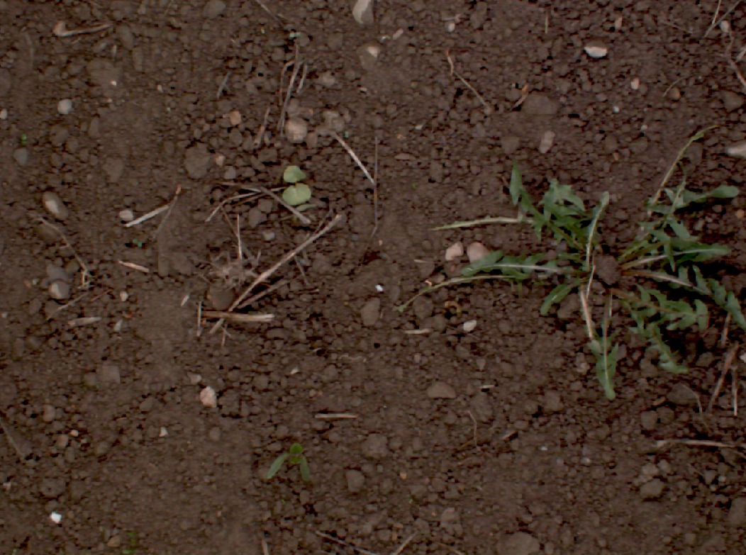
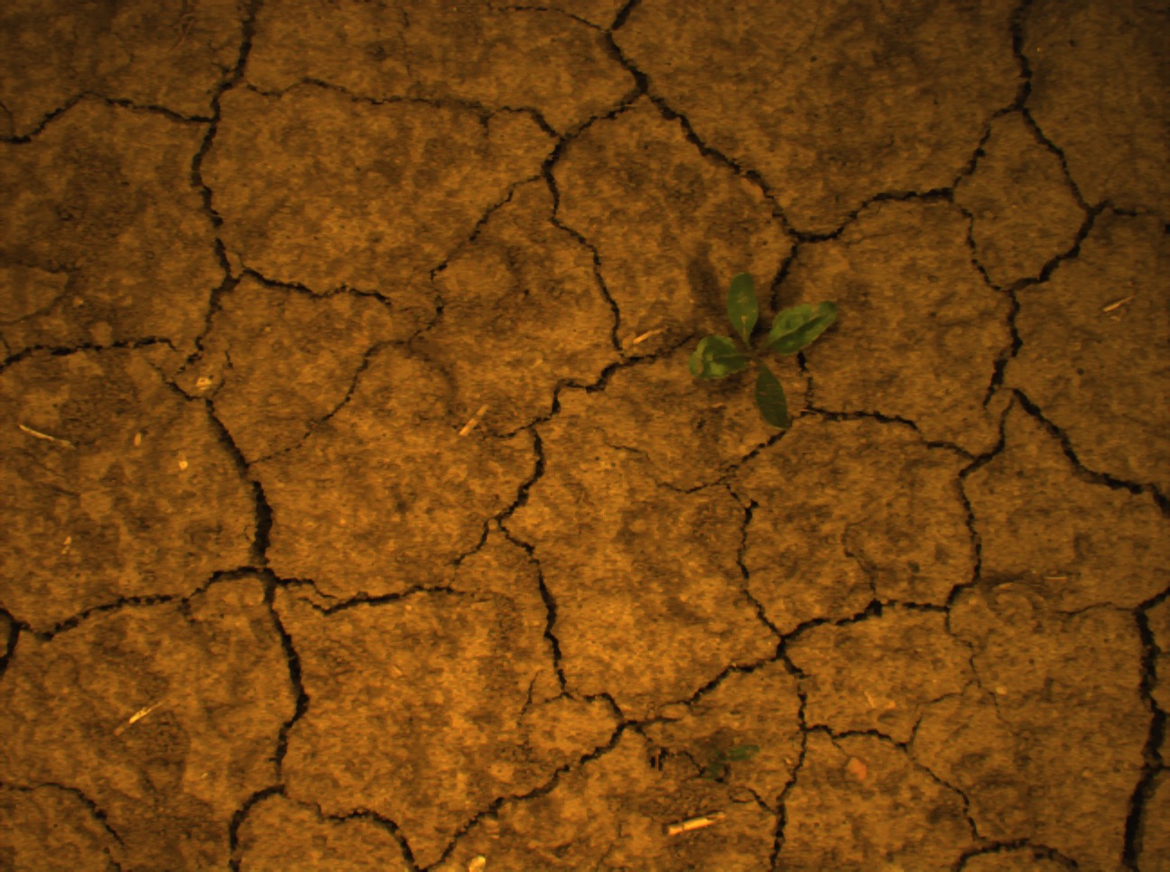
Figure 6: Example images from each dataset. Every dataset contains different crops growth stages, weed types, illumination conditions and soil types. Best viewed in color

IV-B Performance of the Semantic Segmentation

This experiment is designed to support our first claim, which states that our approach can accurately perform pixel-wise semantic segmentation of crops, weeds, and soil, properly dealing with heavy plant overlap in all growth stages.

TABLE III: Pixel-wise Test Sets Performance. Trained in 70% Bonn, reporting 15% held-out Bonn, 100% Stuttgart, and 100% Zurich.

Dataset	Network	mIoU[%]	IoU[%]			Precision[%]			Recall[%]
			Soil	Weeds	Crops	Soil	Weeds	Crops	Soil	Weeds	Crops
Bonn	$\mathcal{I}_{\text{RGB}}$	59.98	99.08	20.64	60.22	99.92	28.97	66.49	99.15	41.79	82.45
	$\mathcal{I}_{\text{RGB}}$+$\mathcal{I}_{\text{NIR}}$	76.92	99.29	49.42	82.06	99.88	52.90	84.19	99.33	88.24	97.01
	$\mathcal{I}_{\text{1}}...\mathcal{I}_{\text{14}}$ (ours)	80.8	99.48	59.17	83.72	99.95	65.92	85.71	99.53	85.25	97.29
Zurich	$\mathcal{I}_{\text{RGB}}$	38.25	96.84	14.26	3.62	96.95	14.96	3.78	96.88	35.35	45.86
	$\mathcal{I}_{\text{RGB}}$+$\mathcal{I}_{\text{NIR}}$	41.23	98.44	16.83	8.43	99.68	19.03	9.07	98.46	51.27	54.46
	$\mathcal{I}_{\text{1}}...\mathcal{I}_{\text{14}}$ (ours)	48.36	99.27	23.40	22.39	99.90	31.43	23.05	99.36	47.79	88.74
Stuttgart	$\mathcal{I}_{\text{RGB}}$	48.09	99.18	21.40	23.69	99.84	21.90	52.43	99.34	42.95	28.95
	$\mathcal{I}_{\text{RGB}}$+$\mathcal{I}_{\text{NIR}}$	55.82	98.54	23.13	45.80	99.85	25.28	68.76	98.69	49.10	57.84
	$\mathcal{I}_{\text{1}}...\mathcal{I}_{\text{14}}$ (ours)	61.12	99.32	26.36	57.65	99.86	37.58	68.77	99.45	46.90	78.09

In Tab. III, we show the pixel-wise performance of the classifier tested in the 15% held out test set from Bonn, as well as the whole datasets from Zurich and Stuttgart. These results show that the network trained using the RGB images in conjunction with the extra computed representations of the inputs outperforms the network using solely RGB images significantly in all categories, performing comparably with the network that uses the extra visual cue from the NIR information, which comes with a high additional cost as specific sensors have to be employed.

Even though the pixel-wise performance of the classifier is important, in order to perform automated weeding it is important to have an object-wise metric for the classifier’s performance. We show this metric in Tab. IV, where we analyze all objects with area bigger than 50 pixels. This number is calculated by dividing our desired minimum object detection size of $1~{}$\mathrm{c}\mathrm{m}^{2}$$ by the spatial resolution of $2~{}$\mathrm{m}\mathrm{m}^{2}$/\text{px}$ in our $512\times 384$ resized images. We can see that in terms of object-wise performance the network using all representations outperforms its RGB counterpart. Most importantly, in the case of generalization to the datasets of Zurich and Stuttgart, this difference becomes critical, since the RGB network yields a performance so low that it renders the classifier unusable for most tasks.

Note that the network using RGB and extra representations is around 30% faster to converge to 95% of the final accuracy than its RGB counterpart, and roughly 15% faster than the network using the NIR channel.

TABLE IV: Object-wise Test Performance. Trained in 70% Bonn, reporting 15% held-out Bonn, 100% Stuttgart, and 100% Zurich.

Dataset	Network	mAcc[%]	Precision[%]		Recall[%]
			Weeds	Crops	Weeds	Crops
Bonn	$\mathcal{I}_{\text{RGB}}$	86.34	83.63	81.14	91.99	80.42
	$\mathcal{I}_{\text{RGB}}$+$\mathcal{I}_{\text{NIR}}$	93.72	90.51	95.09	94.79	89.46
	$\mathcal{I}_{\text{1}}...\mathcal{I}_{\text{14}}$ (ours)	94.74	98.16	91.97	93.35	95.17
Zurich	$\mathcal{I}_{\text{RGB}}$	45.51	59.75	19.71	42.52	23.66
	$\mathcal{I}_{\text{RGB}}$+$\mathcal{I}_{\text{NIR}}$	68.03	67.41	46.78	65.31	49.32
	$\mathcal{I}_{\text{1}}...\mathcal{I}_{\text{14}}$ (ours)	72.08	67.91	72.55	63.33	64.94
Stuttgart	$\mathcal{I}_{\text{RGB}}$	46.05	42.32	42.03	46.1	25.01
	$\mathcal{I}_{\text{RGB}}$+$\mathcal{I}_{\text{NIR}}$	73.99	74.30	70.23	71.35	53.88
	$\mathcal{I}_{\text{1}}...\mathcal{I}_{\text{14}}$ (ours)	76.54	87.87	65.25	64.66	85.15

IV-C Labeling Cost for Adaptation to New Fields

This experiment is designed to support our second claim, which states that our approach can act as a robust feature extractor for images in conditions not seen in the training set, requiring little data to adapt to the new environment.

One way to analyze the generalization performance of the approach is to analyze the amount of data that needs to be labeled in a new field for the classifier to achieve state-of-the-art performance. For this, we separate the Zurich and Stuttgart datasets in halves, and we keep 50% of it for testing. From each of the remaining 50%, we extract sets of 10, 20, 50 and 100 images, and we retrain the last layer of the network trained in Bonn, using the convolutional layers in the encoder and the decoder as a feature extractor. We further separate this small sub-samples in 80%-20% for training and validation and we train until convergence, using early stopping, which means that we stop training when the validation error starts to increase. This is to provide an automated approach to the retraining, so that it can be done without supervision of an expert.

We show the results of the retraining on the Zurich dataset in Tab. VI and Fig. 7, where we can see that the performance of the RGB network when relabeling 100 images is roughly the same as the one using all input representations when the latter is using only 10 images, thus significantly reducing the relabeling effort. We also show that we can get values of precision and recall in the order of 90% when using 100 images for the relabeling in the case of our network, which exploits additional channels. In Tab. VI and Fig. 7, we show the same for the Stuttgart dataset, but in this case the RGB network fails to reach an acceptable performance, while the accuracy of our approach grows linearly with the number of images used.

TABLE V: Object-wise test performance retraining in N images of Zurich dataset.

Inputs	Nr. Images	mAcc[%]	Precision[%]		Recall[%]
			Weeds	Crops	Weeds	Crops
$\mathcal{I}_{\text{RGB}}$	10	60.08	58.75	62.22	73.03	57.99
	20	71.38	61.38	81.42	76.72	64.58
	50	74.08	63.00	85.42	74.14	68.34
	100	82.26	65.50	85.59	74.97	69.91
$\mathcal{I}_{\text{1}}...\mathcal{I}_{\text{14}}$ (ours)	10	83.90	69.23	80.73	71.71	76.18
	20	85.31	75.85	79.12	67.67	84.01
	50	86.25	76.50	85.24	71.55	84.33
	100	89.55	85.89	89.52	89.69	86.76

TABLE VI: Object-wise Test performance retraining in N images of Stuttgart dataset.

Inputs	Nr. Images	mAcc[%]	Precision[%]		Recall[%]
			Weeds	Crops	Weeds	Crops
$\mathcal{I}_{\text{RGB}}$	10	71.76	93.88	52.59	56.57	81.10
	20	72.30	94.40	57.72	51.43	86.35
	50	72.97	94.33	59.70	54.11	87.69
	100	73.34	95.20	63.26	56.36	87.66
$\mathcal{I}_{\text{1}}...\mathcal{I}_{\text{14}}$ (ours)	10	81.40	89.48	64.42	78.74	79.69
	20	81.84	87.83	68.18	81.45	74.61
	50	86.75	94.68	71.34	83.22	90.23
	100	91.88	95.45	86.58	89.08	91.43

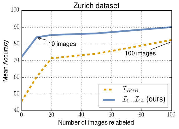
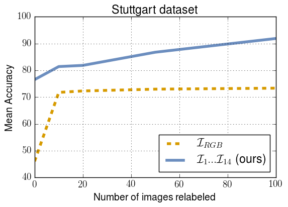
Figure 7: Object-wise mean accuracy vs. relabeling effort. Zero images means no retraining.

IV-D Runtime

This experiment is designed to support our third claim, which states that our approach can be run in real-time, and therefore it can be used for online operation in the field, running in hardware that can be fitted in mobile robots.

We show in Tab. VII that even though the architecture using all extra representations of the RGB inputs has a speed penalty, due to the efficiency of the network we can run the full classifier at more than 20 frames per second on the hardware in our UGV, which consists of an Intel i7 CPU and an NVIDIA GTX1080Ti GPU. Furthermore, we tested our approach in the Jetson TX2 platform, which has a very small footprint and only takes $15\,$\mathrm{W}$$ of peak power, making it suitable for operation on a flying vehicle, and here we still obtain a frame rate of almost $5\,$\mathrm{H}\mathrm{z}$$.

TABLE VII: Runtime in different devices.

Inputs	FLOPS	Hardware	Preproc.	Network	Total	FPS
RGB	$1.8\text{G}$	i7+GTX1080Ti	-	$31$\mathrm{m}\mathrm{s}$$	$31$\mathrm{m}\mathrm{s}$$	$32.2$
		Tegra TX2 SoC	-	$190$\mathrm{m}\mathrm{s}$$	$190$\mathrm{m}\mathrm{s}$$	$5.2$
All	$2\text{G}$	i7+GTX1080Ti	$6$\mathrm{m}\mathrm{s}$$	$38$\mathrm{m}\mathrm{s}$$	$44$\mathrm{m}\mathrm{s}$$	$22.7$
		Tegra TX2 SoC	$6$\mathrm{m}\mathrm{s}$$	$204$\mathrm{m}\mathrm{s}$$	$210$\mathrm{m}\mathrm{s}$$	$4.7$

V Conclusion

In this paper, we presented an approach to pixel-wise semantic segmentation of crop fields identifying crops, weeds, and background in real-time solely from RGB data. We proposed a deep encoder-decoder CNN for semantic segmentation that is fed with a 14-channel image storing vegetation indexes and other information that in the past has been used to solve crop-weed classification tasks. By feeding this additional, task-relevant background knowledge to the network, we can speed up training and improve the generalization capabilities on new crop fields, especially if the amount of training data is limited. We implemented and thoroughly evaluated our system on a real agricultural robot operating using data from three different cities in Germany and Switzerland. Our results suggest that our system generalizes well, can operate at around 20 Hz, and is suitable for online operation in the fields.

References

- [1] V. Badrinarayanan, A. Kendall, and R. Cipolla. Segnet: A deep convolutional encoder-decoder architecture for image segmentation. IEEE Trans. on Pattern Analalysis and Machine Intelligence, 2017.
- [2] N. Chebrolu, P. Lottes, A. Schaefer, W. Winterhalter, W. Burgard, and C. Stachniss. Agricultural Robot Dataset for Plant Classification, Localization and Mapping on Sugar Beet Fields. Intl. Journal of Robotics Research (IJRR), 2017.
- [3] M. Di Cicco, C. Potena, G. Grisetti, and A. Pretto. Automatic model based dataset generation for fast and accurate crop and weeds detection. arXiv preprint, 2016.
- [4] W. Guo, U.K. Rage, and S. Ninomiya. Illumination invariant segmentation of vegetation for time series wheat images based on decision tree model. Computers and Electronics in Agriculture, 96:58–66, 2013.
- [5] D. Hall, C.S. McCool, F. Dayoub, N. Sunderhauf, and B. Upcroft. Evaluation of features for leaf classification in challenging conditions. In Proc. of the IEEE Winter Conf. on Applications of Computer Vision (WACV), pages 797–804, Jan 2015.
- [6] E. Hamuda, M. Glavin, and E. Jones. A survey of image processing techniques for plant extraction and segmentation in the field. Computers and Electronics in Agriculture, 125:184–199, 2016.
- [7] S. Haug, A. Michaels, P. Biber, and J. Ostermann. Plant classification system for crop / weed discrimination without segmentation. In Proc. of the IEEE Winter Conf. on Applications of Computer Vision (WACV), pages 1142–1149, 2014.
- [8] K. He, G. Gkioxari, P. Dollár, and R. Girshick. Mask R-CNN. arXiv preprint, 2017.
- [9] K. He, X. Zhang, S. Ren, and J. Sun. Deep residual learning for image recognition. In Proc. of the IEEE Conf. on Computer Vision and Pattern Recognition (CVPR), 2016.
- [10] P. Lottes, M. Hoeferlin, S. Sanders, and C. Stachniss. Effective Vision-Based Classification for Separating Sugar Beets and Weeds for Precision Farming. Journal of Field Robotics (JFR), 2016.
- [11] P. Lottes, H. Markus, S. Sander, M. Matthias, S.L. Peter, and C. Stachniss. An Effective Classification System for Separating Sugar Beets and Weeds for Precision Farming Applications. In Proc. of the IEEE Intl. Conf. on Robotics & Automation (ICRA), 2016.
- [12] P. Lottes and C. Stachniss. Semi-supervised online visual crop and weed classification in precision farming exploiting plant arrangement. In Proc. of the IEEE/RSJ Intl. Conf. on Intelligent Robots and Systems (IROS), 2017.
- [13] C.S. McCool, T. Perez, and B. Upcroft. Mixtures of Lightweight Deep Convolutional Neural Networks: Applied to Agricultural Robotics. IEEE Robotics and Automation Letters (RA-L), 2017.
- [14] G.E. Meyer and J. Camargo Neto. Verification of color vegetation indices for automated crop imaging applications. Computers and Electronics in Agriculture, 63(2):282 – 293, 2008.
- [15] A. Milioto, P. Lottes, and C. Stachniss. Real-time blob-wise sugar beets vs weeds classification for monitoring fields using convolutional neural networks. In Proc. of the Intl. Conf. on Unmanned Aerial Vehicles in Geomatics, 2017.
- [16] A.K. Mortensen, M. Dyrmann, H. Karstoft, R. N. Jörgensen, and R. Gislum. Semantic segmentation of mixed crops using deep convolutional neural network. In Proc. of the International Conf. of Agricultural Engineering (CIGR), 2017.
- [17] A. Paszke, A. Chaurasia, S. Kim, and E. Culurciello. Enet: Deep neural network architecture for real-time semantic segmentation. arXiv preprint, abs/1606.02147, 2016.
- [18] M.P. Ponti. Segmentation of low-cost remote sensing images combining vegetation indices and mean shift. IEEE Geoscience and Remote Sensing Letters, 10(1):67–70, Jan 2013.
- [19] C. Potena, D. Nardi, and A. Pretto. Fast and accurate crop and weed identification with summarized train sets for precision agriculture. In Proc. of Int. Conf. on Intelligent Autonomous Systems (IAS), 2016.
- [20] F.M. De Rainville, A. Durand, F.A. Fortin, K. Tanguy, X. Maldague, B. Panneton, and M.J. Simard. Bayesian classification and unsupervised learning for isolating weeds in row crops. Pattern Analysis and Applications, 17(2):401–414, 2014.
- [21] J. Torres-Sanchez, F. López-Granados, and J.M. Peña. An automatic object-based method for optimal thresholding in uav images: Application for vegetation detection in herbaceous crops. Computers and Electronics in Agriculture, 114:43 – 52, 2015.
- [22] A. Wendel and J.P. Underwood. Self-Supervised Weed Detection in Vegetable Crops Using Ground Based Hyperspectral Imaging. In Proc. of the IEEE Intl. Conf. on Robotics & Automation (ICRA), 2016.