Market Dynamics. On A Muse Of Cash Flow And Liquidity Deficit.

Abstract

$Id: AMuseOfCashFlowAndLiquidityDeficit.tex,v 1.575 2019/03/28 06:02:45 mal Exp $

A first attempt at obtaining market–directional information from a non–stationary solution of the dynamic equation ‘‘future price tends to the value that maximizes the number of shares traded per unit time’’ Malyshkin and Bakhramov (2015) is presented. We demonstrate that the concept of price impact is poorly applicable to market dynamics. Instead, we consider the execution flow $I=dV/dt$ operator with the ‘‘impact from the future’’ term providing information about not–yet–executed trades. The ‘‘impact from the future" on $I$ can be directly estimated from the already–executed trades, the directional information on price is then obtained from the experimentally observed fact that the $I$ and $p$ operators have the same eigenfunctions (the exact result in the dynamic impact approximation $p=p(I)$). The condition for ‘‘no information about the future’’ is found and directional prediction quality is discussed. This work makes a substantial contribution toward solving the ultimate market dynamics problem: find evidence of existence (or proof of non–existence) of an automated trading machine which consistently makes positive P&L on a free market as an autonomous agent (aka the existence of the market dynamics equation). The software with a reference implementation of the theory is provided.

I Introduction

Market Dynamics is the central concept of modern economic study. An ultimate form of the study to be an evidence of existence (or a proof of non–existence) of an automated trading machine, consistently making positive P&L (with a given value of risk) trading on a free market as an autonomous agent. In our previous studyMalyshkin (2016); Malyshkin and Bakhramov (2016) we have shown experimentally that supply and demand match each other down to milliseconds time scale, thus their disbalance cannot be a source of market dynamics. Moreover, supply and demand cannot be measured or estimated from the data even after transaction executionMalyshkin (2016). In the modern world all available data is typically represented in a form of recorded transactions, where money, financial instruments, goods, etc. change hands. In each such transaction there are two matched parties (e.g. ‘‘A’’ sold $x$ goods to ‘‘B’’ and received $y$ dollars for that) what means that in recorded data supply and demand are matched. The disbalance of supply/demand cannot (even in principle!) be measured from a sequence of transactions, as any transaction assume the parties to match. An example of information source, that is not a sequence of transactions, is the Limit Order Book. However, using Limit Order Book as a source of information about Supply and Demand is fruitlessMalyshkin and Bakhramov (2016) since at least 2008–2010 and exchange trading is now little different from dark pool trading. (We tried to consider the Limit Order Book both: as not a sequence of transaction, and as a sequence of add/{cancel$|$execute} transactions, but without much success; most typical limit order book pattern is: added order spend almost no time in the order book, it either get almost immediately executed or canceled. The ratio observed is that more than 90% of orders being at best price level at some time end up being canceledHautsch and Huang (2011); Malyshkin and Bakhramov (2015). This is due to exchange fee structure, because add/cancel order ‘‘round trip’’ cost (almost) no money and carry little risk for market participants.) This make us to conclude that the disbalance of supply and demand is not a practically applicable concept, because it cannot be measured from recorded transactions.

For practical applications we need a concept that can be estimated from a sequence of transactions. In Malyshkin (2016); Malyshkin and Bakhramov (2015) a concept of execution flow ($I=dV/dt$ a number of shares traded in unit time, a number of dollars paid in unit time, etc.) was introduced and practical approach to its calculation (based on Radon–Nikodym derivatives and their generalization) was developed.

An application of this approach in quasistationary case was demonstrated in Malyshkin (2016), where we have shown that asset price is much more sensitive to execution rate $I=dV/dt$, rather than to trading volume $V$, and dynamic impact (sensitivity to $I$) was introduced as a practical alternative to regular impactWikipedia (2016a) (sensitivity to $V$). In this paper we make one more step forward, demonstrating an application of this approach in a non–stationary case. First, we show that price impact, the central subject of many studies, is poorly applicable to market dynamics. A practical alternative to it is an impact from the future on $I$, that can be estimated from past sample. Then we are trying to obtain directional information on price from a knowledge of future $I$, with the goal to obtain trading strategy with a positive P&L. There is a fundamental philosophical questionBoiko and Malyshkin (27 Feb. 2009) about positive P&L provided by an automated trading machine: Assume one created a ‘‘Real Time Machine’’, but looking only very few moments ahead in the future. How to prove that a given ‘‘Time Machine’’ works? Attach it to an exchange and show the P&L! In this sense any dynamic equation (Newton, Maxwell, Schrödinger) can be considered as some kind of ‘‘Time Machine’’. Moreover, any intelligence can be considered as a ‘‘future prediction system’’ Hawkins and Blakeslee (2007), thus, when applied to the market, the P&L can be considered as an ‘‘intelligence criteria’’ of an automated trading machine. There is a very deep difference between an intelligent agent and statistical approach. For an intelligent agent a single observation is enough to make a prediction. For any statistical approach a large number of observations is required to make any kind of inference. In Malyshkin and Bakhramov (2016) we emphasized the inapplicability of any statistical approach to exchange trading and the importance of the dynamical approach, a practical alternative to a statistical one.

The dynamic equation we introducedMalyshkin and Bakhramov (2015) ‘‘future price tends to the value that maximizes the number of shares traded per unit time’’ in this direct form requires to know ‘‘future’’ prices and flows, and can be easily solved only in quasistationary caseMalyshkin (2016). In a non–stationary case the best result of our previous studyMalyshkin and Bakhramov (2015) was ‘‘maximizing the number of shares traded per unit time on past observations sample’’, but with a limited success. The concept of market dynamics in its ultimate form requires to determine future market movement from past observations sample. In this paper a substantial progress is made toward this goal. In Section VII an estimation (45) of the impact from the future on $I$ is made, allowing (from experimentally observedMalyshkin (2016) fact that $I$ and $p$ operators to have the same eigenfunctions, at least for the states with high $I$) to obtain price directional answer. This dynamic equation solution is equivalent to some trending model, but have an automatic selection of the relevant time scale, a critically important feature of any automated trading systemMalyshkin and Bakhramov (2015).

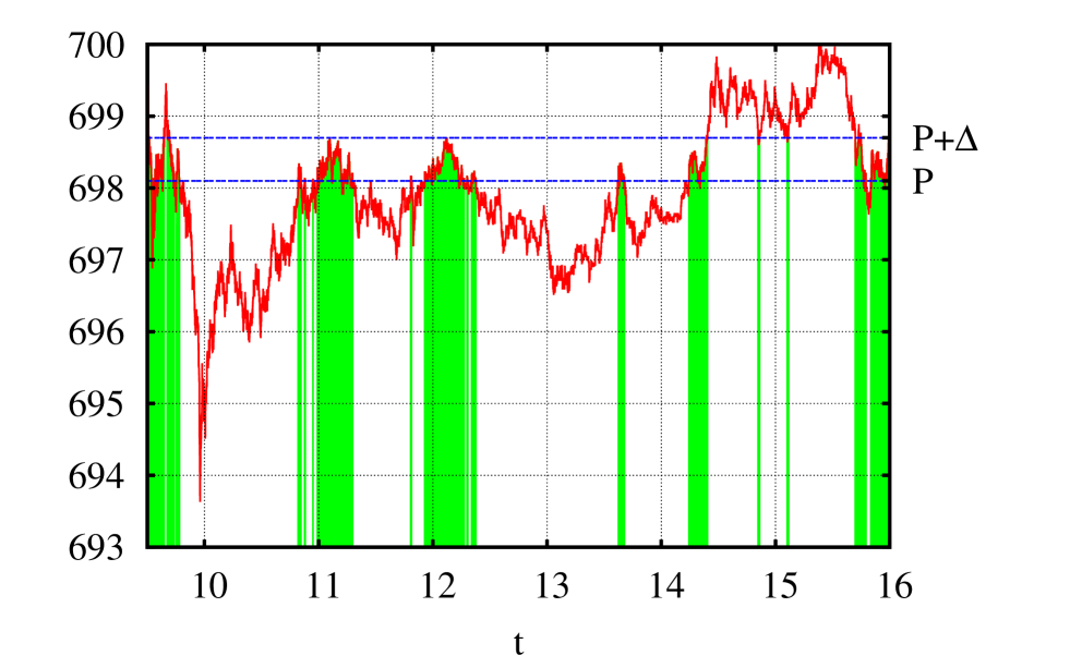
In Ref. Malyshkin and Bakhramov (2015), as a first application of the dynamic equation, the concept of liquidity deficit trading was introduced: open a position on low $I_{0}$ ($I_{0}$ is defined in Eq. (41)), close already opened position on high $I_{0}$, as the only way to build a strategy, resilient to catastrophic P&L loss. In Ref. Malyshkin and Bakhramov (2015) market directional information was not obtained, thus only volatility trading was available for practical implementation. In this new study we made a substantial progress in dynamic equation application: to obtain market directional information from the dynamic equation.

Computer code with a reference implementation of the theory is presented in the Appendix G.

II Basis Selection

To operate with introduced inMalyshkin and Bakhramov (2015) concepts we need to convert market observable timeserie variables (time, execution price, shares traded) to a set of distribution moments. The three bases, performing time averaging with the exponential weight, are the most convenient for market dynamics study. Laguerre basis:

$$x = t/\tau$$ (1)

$$x_{0} = 0$$ (2)

$$\Braket{Q_{k}f} = \int\limits_{-\infty}^{x_{0}}Q_{k}(x)f(t)\exp(x)dx$$ (3)

$$d\mu = \exp(x)dx$$ (4)

$$\mathrm{supp}(\mu(x)) = x\in[-\infty,x_{0}]$$ (5)

$$D(Q_{k}(x)) = \frac{dQ_{k}(x)}{dx}+\frac{Q_{k}(x)}{2}$$ (6)

$$\Braket{Q_{k}f} = \sum_{i}Q_{k}(-\frac{t_{now}-t_{i}}{\tau})\exp(-\frac{t_{now}-t_{i}}{\tau})f(t_{i})\frac{t_{i}-t_{i-1}}{\tau}$$ (7)

Shifted Legendre basis:

$$x = \exp(t/\tau)$$ (8)

$$x_{0} = 1$$ (9)

$$\Braket{Q_{k}f} = \int\limits_{-\infty}^{0}Q_{k}(x)f(t)\exp(t/\tau)dt/\tau=\int\limits_{0}^{x_{0}}Q_{k}(x)f(t)dx$$ (10)

$$d\mu = \exp(t/\tau)dt/\tau=dx$$ (11)

$$\mathrm{supp}(\mu(x)) = x\in[0,x_{0}]$$ (12)

$$D(Q_{k}(x)) = x\frac{dQ_{k}(x)}{dx}+\frac{Q_{k}(x)}{2}$$ (13)

$$\Braket{Q_{k}f} = \sum_{i}Q_{k}(\exp(-\frac{t_{now}-t_{i}}{\tau}))\exp(-\frac{t_{now}-t_{i}}{\tau})f(t_{i})\frac{t_{i}-t_{i-1}}{\tau}$$ (14)

Price Basis

$$x = p$$ (15)

$$\Braket{Q_{k}f} = \int\limits_{-\infty}^{0}Q_{k}(p(t))f(t)\exp(t/\tau)dt/\tau$$ (16)

$$d\mu = \exp(t/\tau)dt/\tau$$ (17)

$$\mathrm{supp}(\mu(p(t))) = t\in[-\infty,0]$$ (18)

$$\Braket{Q_{k}f} = \sum_{i}Q_{k}(p(t_{i}))\exp(-\frac{t_{now}-t_{i}}{\tau})f(t_{i})\frac{t_{i}-t_{i-1}}{\tau}$$ (19)

$Q_{k}(x)$ is a polynomial of $k$–th order (e.g. monomials $\{1;x;x^{2};x^{3};\dots\}$), but from numerical stability pointMalyshkin and Bakhramov (2015) for (4) a good choice is the selection $Q_{k}(x)=L_{k}(-x)$, with $L_{k}(x)$ Laguerre polynomials, and for (11) a good choice is the selection $Q_{k}(x)=P_{k}(2x-1)$, with $P_{k}(x)$ Legendre polynomials. This choice make the basis orthogonal in $d\mu$ measure: $\int_{0}^{\infty}L_{j}(x)L_{k}(x)\exp(-x)dx=\delta_{jk}$ and $\int_{0}^{1}P_{j}(2x-1)P_{k}(2x-1)dx=\frac{1}{2k+1}\delta_{jk}$, what drastically increase the numerical stability of calculations. However, all results are invariant with respect to polynomials selection. The specific choice affects only numerical stability of calculations, thus should be discussed separatelyLaurie and Rolfes (1979); Beckermann (1996); Malyshkin and Bakhramov (2015); Malyshkin (2015a). Proper basis selectionMalyshkin (2015a) allows us to have the numerically stable results even for two–dimensional basis with 100 basis functions in each dimension, i.e. with 10000 basis functions total for 64bit double precision computer arithmetic.

The Eqs. (7), (14) and (19) show how to calculate the $\Braket{Q_{k}f}$ moments from a timeserie sample $f(t_{i})$. To simplify working with averages introduce quantum mechanic bra–ket notationWikipedia (2016b) $\Bra{}$ and $\Ket{}$:

$$\Braket{Q_{k}f} = \int d\mu Q_{k}(x)f(t)$$ (20)

$$\Braket{Q_{j}}{f}{Q_{k}} = \int d\mu Q_{j}(x)Q_{k}(x)f(t)$$ (21)

where the integral $\int d\mu$ in (21) is calculated directly from a timeserie according to (7), (14) or (19) depending on basis used. Familiar values can be easily presented with these definitions. Price exponential moving average: put price at time $t_{i}$ as the $f(t_{i})$, then $\overline{p}_{\tau}=\Braket{Q_{0}p}/\Braket{Q_{0}}$ is required moving average. From all the considerations above one can easily see that bra–ket $\Bra{}$ and $\Ket{}$ notations from quantum mechanic are nothing more, than a ‘‘glorified moving average’’, and think of $\Braket{Q_{k}}{f}{Q_{j}}$ as taking a moving average with two basis functions product: $\int d\mu Q_{k}(x(t))f(t)Q_{j}(x(t))$. Different $d\mu$ measures can be defined in a similar way. However the measures (4) and (11) are specialLaurie (14 Nov. 2015), in a sense they allow to calculate the $\Braket{Q_{k}df/dt}$ moments from the $\Braket{Q_{k}f}$ moments using integration by parts. The following condition also holds:

$$Q_{j}(x_{0})Q_{k}(x_{0})=\Braket{Q_{j}(x)D\left(Q_{k}(x)\right)}+\Braket{D\left(Q_{j}(x)\right)Q_{k}(x)}$$ (22)

Infinitesimal time–shift linear operator $D(\psi(x))$ from (6) and (13), is different from plain differentiation because exponent differentiation in (4) and (11) give an extra term. The selection of basis functions as a function of price $Q_{k}(p(t))$ in (17) is extremely convenient in the quasistationary caseMalyshkin (2016) but does not possess such a simple infinitesimal time–shift transform.

II.1 $I=dV/dt$ as Radon Nikodym Derivative of Lebesgue Measures.

Figure 1: The AAPL stock price on September, 20, 2012. Demonstration of Lebesgue Integral concept: time spent or volume traded with price inside $[P:P+\Delta P]$ interval.

In this subsection we demonstrate price basis convenience for execution flow calculation in the quasistationary case and it’s relation to Radon–Nikodym derivatives, the main technique of our Malyshkin (2016, 2018) papers. The idea is to split price range on a number of $\Delta P$ intervals, then, for each interval calculate:

• time spent

• volume traded

of timeserie observations when the price is inside the $[P:P+\Delta P]$ interval, see Fig. 1 for illustration. These calculations give us two Lebesgue measures: $\Delta t=\mu_{t}(P)\Delta P$ and $\Delta V=\mu_{V}(P)\Delta P$. These measures give time spend and volume traded when the price is inside the range $[P:P+\Delta P]$. By itself these two Lebesgue measures are very similar to each other and are nothing more than a ‘‘glorified price–volume distributions’’, both having distribution maximum near price median, see Fig. 3 (top) of Ref. Malyshkin (2016). But when one take a ratio of these two measures, it gives trades execution flow $I(P)=\mu_{V}(P)/\mu_{t}(P)$, with singularities near price tipping points, see Fig. 3 (center) of Ref. Malyshkin (2016). The execution rate, the central concept of our theory, $I(P)=\mu_{V}(P)/\mu_{t}(P)$ can be considered as Radon–Nikodym derivative of two Lebesgue measures $\mu_{t}(P)\Delta P$ and $\mu_{V}(P)\Delta P$. For numerical calculations the described above histogram–like procedure works well only if discretization scale $\Delta P$ is properly chosen, what is a non–issue for manual analysis, but can be a real problem for an automated system. From numerical perspective there is a much better way to calculate Radon–Nikodym derivative of two measures, a calculation from distribution moments, see the formula (28) below, the answer in the form of Nevai operatorNevai (1986). Given sufficient number of moments (what may be a problem to calculate numerically, unless a stable basis is chosenMalyshkin and Bakhramov (2015)) the (28) is a superior numerical estimator of Radon–Nikodym derivatives.

III Wavefunction

Introduce a wavefunction $\psi(x)$ to be a linear combination of basis function $Q_{k}(x)$ (here $n$ is time–space dimension, typically $n$ take some value between 4 and 20).

$$\psi(x) = \sum\limits_{k=0}^{n-1}\alpha_{k}Q_{k}(x)$$ (23)

Then any observable (or calculable) market–related value $f_{\psi}$, corresponding to a probability density $\psi^{2}(x)$ can be calculated as:

$$f_{\psi} = \frac{\Braket{\psi}{f}{\psi}}{\Braket{\psi}{\psi}}$$ (24)

$$f_{\psi} = \frac{\sum\limits_{j,k=0}^{n-1}\alpha_{j}\Braket{Q_{j}}{f}{Q_{k}}\alpha_{k}}{\sum\limits_{j,k=0}^{n-1}\alpha_{j}\Braket{Q_{j}}{Q_{k}}\alpha_{k}}$$ (25)

The (24) is plain ratio of two moving averages, but the weight is not just a regular decaying exponent according to (4) or (11), but exponent, multiplied by the $\psi^{2}(x)$, thus the $\psi^{2}(x)$ define how to average a timeserie sample $f(t_{i})$. The (25) is (24) with parentheses expanded according to (23). This way any $\psi(x)$ function is defined by $n$ coefficients $\alpha_{k}$, and the value of any observable variable, corresponding to this $\psi(x)$ state is a ratio of two quadratic forms (built on $\alpha_{k}$ coefficients) of dimension $n$, an estimator of stable formMalyshkin (2009). The representation of an observable in a form of two quadratic forms ratio (25) is conceptually different from the representation of an observable in a form of linear superposition of basis functions. In (25) a wavefunction $\psi(x)$ is represented as a linear superposition of basis functions, the $\psi^{2}(x)d\mu$ define probability density, then $f_{\psi}$ is calculated as $f(t_{i})$ averaged with this probability densityBobyl et al. (2016). This approach allows do decouple variables determining market dynamics and variables determined by market dynamics, what is critically important for any market dynamics study.

III.1 Interpolation Example

Given the definitions above, let us show some familiar answers. Let $f(t)$ be some function, obtain $\beta_{k}$, such as the interpolation $A_{LS}(y(t))=\sum_{k=0}^{n-1}\beta_{k}Q_{k}(y(t))$, minimize least squares norm: $\Braket{\left(f(x(t))-\sum_{k=0}^{n-1}\beta_{k}Q_{k}(x(t))\right)^{2}}\to\min$. Taking the derivatives of the norm on $\beta_{k}$ obtain the solution:

$$A_{LS}(y) = \sum\limits_{j,k=0}^{n-1}Q_{j}(y)(G^{-1})_{jk}\Braket{fQ_{k}}$$ (26)

Here $G^{-1}$ is the inverse to Gramm matrix $G_{jk}=\Braket{Q_{j}}{Q_{k}}$ and the (26) is a regular least squares solution, a polynomial of $n-1$ order, where the coefficients are obtained as the solution of a linear system with Gramm matrix.

A much more interesting case is to obtain probability density $\psi^{2}_{y}(x)d\mu$, which is localized at given $y$, then calculate $A_{RN}(y)=\frac{\int f(x)\psi^{2}_{y}(x)d\mu}{\int\psi^{2}_{y}(x)d\mu}$, using probability density with interpolated $\psi_{y}(x)$. There are several formsMalyshkin and Bakhramov (2015) of such localized $\psi_{y}(x)$, the simplest one give (28), Nevai operatorNevai (1986):

$$\psi_{y}(x) = \sum\limits_{j,k=0}^{n-1}Q_{j}(y)(G^{-1})_{jk}Q_{k}(x)$$ (27)

$$A_{RN}(y) = \frac{\sum\limits_{j,k,l,m=0}^{n-1}Q_{j}(y)(G^{-1})_{jk}\Braket{Q_{k}}{f}{Q_{l}}(G^{-1})_{lm}Q_{m}(y)}{\sum\limits_{j,k=0}^{n-1}Q_{j}(y)(G^{-1})_{jk}Q_{k}(y)}$$ (28)

The (27) is interpolated localized wavefunction (localized at $y$, compare it to $A_{LS}$ interpolation (26)), then this localized at $y$ probability density is put to (25) to obtain (28), that is now considered as Radon–Nikodym interpolation of $f$ at $y$. In contrast with the least squares answer (26) (which is a linear combination of basis functions), the (28) is a ratio of two quadratic forms of basis functions, a ratio of two polynomials $2n-2$ order each in case of polynomial basis. The (28) is used for numerical estimation of $\frac{d\nu}{d\mu}=\frac{f(x)d\mu}{d\mu}$, considered as Radon–Nikodym derivative. The (28) answer (basis–invariant answers (26) and (28) take very simple formMalyshkin and Bakhramov (2015); Bobyl et al. (2016) in the basis of eigenfunctions of operator, generated by the $f$), is typically the most convenient one among other available, because it requires only one measure to be positive. Other answersSimon (2011); Malyshkin and Bakhramov (2015) require both measures to be positive. Radon–Nikodym interpolation (28) has several critically important advantagesMalyshkin and Bakhramov (2015); Malyshkin (2015a, b) compared to the least squares interpolation (26): stability of interpolation, there is no divergence outside of interpolation interval, oscillations near interval edges are very much suppressed, even in multi–dimensional caseMalyshkin (2015a). These advantages come from the very fact, that probability density is interpolated first, then the result is obtained by averaging with this, always positive, interpolated probability.

III.2 Probability States

Considered in subsection III.1 localized wavefunction give a simple example, illustrating the power of the technique. However, much more interesting results can be obtained considering not only localized states such as (27), but arbitrary $\psi(x)$. This allows us to decouple observable variables and probability state.

As we emphasized inMalyshkin and Bakhramov (2015) system dynamics cannot be obtained from price. The price is secondary and typically fluctuates few percent a day in contrast with the liquidity flow, that fluctuates in orders of magnitude. (This also allows to estimate maximal workable time scale for an automated trading machine: the scale on which execution flow fluctuates at least in an order of magnitude. Minimal time scale is typically determined by available market liquidityMalyshkin and Bakhramov (2016)). The main idea is to obtain the state $\psi$ from the variables, determining the dynamics (e.g. execution flow $I=dV/dt$, execution flow changes $dI/dt$, etc.) and then use obtained state to determine the values of interest (e.g. price, price change, or P&L). A critically important feature of this approach is that both: the variables determining the dynamics and the variables determined by the dynamics can be directly calculated from recorded data, what is drastically different from Supply–Demand approach, where the disbalance of it cannot be calculated from recorded transactions data, because in all recorded transactions Supply and Demand are matched.

IV Price Impact

Price impact Moro et al. (2009); Gatheral and Schied (2013); Donier et al. (2014) is typically considered as path–dependent impact of executed shares number on asset price. However the price can be affected by a number of other factors and, moreover, an impact defined in such a way may diverge or even do not exist. In a style of previous section, define price impact as price change in a given $\psi(x)$ state. With the approach we develop in this paper price impact is calculated in two steps. First, find the state of interest $\psi(x)$ (e.g. corresponding to a large $I$ or $dI/dt$, etc.). Second calculate price change corresponding to the $\psi(x)$ found on the first step. We define price change, corresponding to the $\psi(x)$, as generalized price impact in the $\psi$ state: $\Delta_{\psi}P$. The selection of $\psi(x)$ will be discussed in the next section. In this section we only demonstrate how to calculate price impact for a given $\psi(x)$. There are two practical answers:

1. The moments $\Braket{Q_{k}dp/dt}$ can be directly calculated from a sample using (7), (14) or (19) with the replacement of the factor $f(t_{i})(t_{i}-t_{i-1})/\tau$ by the factor $(p(t_{i})-p(t_{i-1}))/\tau$. After the calculation of $\Braket{Q_{k}dp/dt}$ moments the $\Delta_{\psi}P$ can be obtained directly:

$$\Delta_{\psi}P = \frac{\Braket{\psi}{\frac{dp}{dt}}{\psi}}{\Braket{\psi}{\psi}}=\frac{\sum\limits_{j,k=0}^{n-1}\alpha_{j}\Braket{Q_{j}}{\frac{dp}{dt}}{Q_{k}}\alpha_{k}}{\sum\limits_{j,k=0}^{n-1}\alpha_{j}\Braket{Q_{j}}{Q_{k}}\alpha_{k}}$$ (29)

The (29) give an answer calculated directly from sample.

2. In some situations the moments $\Braket{Q_{k}dp/dt}$ are not convenient to use or not available and only $\Braket{Q_{k}pI}$ sampled moments are available. Then calculate the price $p_{\psi}$, corresponding to the $\psi(x)$ state, and variate $\psi(x)$ using infinitesimal time–shift operator $D(\psi)$ from (6) or (13) depending on the basis used.

$$p_{\psi} = \frac{\Braket{\psi}{pI}{\psi}}{\Braket{\psi}{I}{\psi}}$$ (30)

$$\Delta_{\psi}P = -2\left(\frac{\Braket{D(\psi)}{pI}{\psi}}{\Braket{\psi}{I}{\psi}}-\frac{\Braket{\psi}{pI}{\psi}}{\Braket{\psi}{I}{\psi}}\frac{\Braket{D(\psi)}{I}{\psi}}{\Braket{\psi}{I}{\psi}}\right)$$ (31)

The (31) is the first order variation of Rayleigh quotient (30), the second order variation of Rayleigh quotient can be also calculated, see the (180) below with $\delta\psi=-D(\psi)$, but note that that $D(D(\psi))$ terms need to be added to (183) in general case.

The (29) and (31) may or may not give similar answer, because they treat the boundary $x=x_{0}$ (time is ‘‘now’’) differently. Substantial difference in between (29) and (31) typically indicates a large contribution of the boundary, and is a signal of possible discrepancy in generalized price impact estimation. But, as we emphasized earlierMalyshkin and Bakhramov (2015), in practical applications other than price, dynamics–related attributes (e.g. P&L or $I$) should be considered instead.

V Wavefunction States Important For Market Dynamics

Localized $\psi$ state, considered in the subsection III.1, is of interest for interpolation problem only. For dynamic problem other $\psi$ to be considered. There is a number of interesting situations to consider, but consider the two forms of $\psi$, the most promising for market dynamics and for generalized price impact calculation.

V.1 $\psi$ Corresponding to Maximal $I$

We have already emphasizedMalyshkin (2016) the importance of the states, corresponding to maximal $I$. The problem of maximizing $I$ on ‘‘past’’ sampleMalyshkin and Bakhramov (2015) can be reduced to a generalized eigenvalue problem (33).

$$\frac{\Braket{\psi}{I}{\psi}}{\Braket{\psi}{\psi}} \to \max$$ (32)

$$\sum\limits_{k=0}^{n-1}\Braket{Q_{j}}{I}{Q_{k}}\alpha^{[i]}_{k} = \lambda_{I}^{[i]}\sum\limits_{k=0}^{n-1}\Braket{Q_{j}}{Q_{k}}\alpha^{[i]}_{k}$$ (33)

$$\psi^{[i]}_{I}(x) = \sum\limits_{k=0}^{n-1}\alpha^{[i]}_{k}Q_{k}(x)$$ (34)

Generalized eigenvalue problem (33) provide $n$ solutions ($i=[0\dots n-1]$), each $i$ corresponds to the (eigenvalue,eigenfunction) pair $(\lambda_{I}^{[i]},\psi^{[i]}_{I}(x))$. The state $\psi^{[IH]}_{I}(x)$, corresponding to the maximal $\lambda_{I}$, is a first good candidate for generalized price impact calculation.

V.2 $\psi$ Corresponding to Maximal $dI/dt$

The state, corresponding to maximal $dI/dt$ can be also of interest for market dynamics. In contrast with the $\Braket{Q_{j}}{dp/dt}{Q_{k}}$, $\Braket{Q_{j}}{I}{Q_{k}}$ and $\Braket{Q_{j}}{pI}{Q_{k}}$ matrices the matrix $\Braket{Q_{j}}{dI/dt}{Q_{k}}$ cannot be directly calculated from sample. However, in a presence of an infinitesimal time–shift operator (22) this matrix can be calculated by applying integration by parts:

$$\Braket{Q_{j}\left missing}{\frac{dI}{dt}}{Q_{k}} = I^{f}Q_{j}(x_{0})Q_{k}(x_{0})-\Braket{D(Q_{j})}{I}{Q_{k}}-\Braket{Q_{j}}{I}{D(Q_{k})}$$ (35)

Edge $x=x_{0}$ value $I^{f}$ is unknown in general case. We have tried various values for $I^{f}$, but for simplicity of calculation let us put $I^{f}=0$ in this section (see the Section VII below for the case $I^{f}=\lambda_{I}^{[IH]}$). The $I^{f}=0$ means that the trading ‘‘now’’ is expected to stop at this price. Then the $\Braket{Q_{j}}{dI/dt}{Q_{k}}$ matrix can be obtained from (35) and generalized eigenvalue problem can be written in a usual way:

$$\frac{\Braket{\psi\left missing}{\frac{dI}{dt}}{\psi}}{\Braket{\psi}{\psi}} \to \max$$ (36)

$$\sum\limits_{k=0}^{n-1}\Braket{Q_{j}\left missing}{\frac{dI}{dt}}{Q_{k}}\alpha^{[i]}_{k} = \lambda_{dI}^{[i]}\sum\limits_{k=0}^{n-1}\Braket{Q_{j}}{Q_{k}}\alpha^{[i]}_{k}$$ (37)

$$\psi^{[i]}_{dI}(x) = \sum\limits_{k=0}^{n-1}\alpha^{[i]}_{k}Q_{k}(x)$$ (38)

Generalized eigenvalue problem (37) provide $n$ solutions ($i=[0\dots n-1]$), each $i$ corresponds to the (eigenvalue,eigenfunction) pair $(\lambda_{dI}^{[i]},\psi^{[i]}_{dI}(x))$. The state $\psi^{[dIH]}_{dI}(x)$, corresponding to the maximal $\lambda_{dI}$, is a second good candidate for generalized price impact calculation.

V.3 $\psi$ Localized at $x_{0}$

Localized at $x_{0}$ (the state ‘‘time is now’’) the wavefunction $\psi_{0}(x)$ is of ‘‘interpolatory’’ type and does not provide any valuable information about market dynamics but is useful in some applications. Take (27) and put $y=x_{0}$ to obtain the $\psi_{0}(x)$. In Malyshkin (2016); Malyshkin and Bakhramov (2015), just for convenience, we used normalized $\psi_{0}(x)$:

$$\psi_{0}(x) = \frac{\sum\limits_{j,k=0}^{n-1}Q_{j}(x_{0})(G^{-1})_{jk}Q_{k}(x)}{\sqrt{\sum\limits_{j,k=0}^{n-1}Q_{j}(x_{0})(G^{-1})_{jk}Q_{k}(x_{0})}}$$ (39)

$$1 = \Braket{\psi_{0}}{\psi_{0}}$$ (40)

The (39) is plain normalized (27), normalization factor cancels in the numerator and in the denominator of (24) when calculating an observable.

VI Demonstration Of Generalized Price Impact Calculation

Figure 2: The AAPL stock price on September, 20, 2012. Calculated in Shifted Legendre basis with $n=7$ and $\tau$=128sec. Calculations are performed using $dp$ moments ($direct$, Eq. (29)) and $pI$ moments ($var\,pI$, Eq. (31)). Top: Generalized Price Impact on $\psi$ state, corresponding to the maximal $I$, (32). Bottom: Generalized Price Impact on $\psi$ state, corresponding to the maximal $dI/dt$, (36).

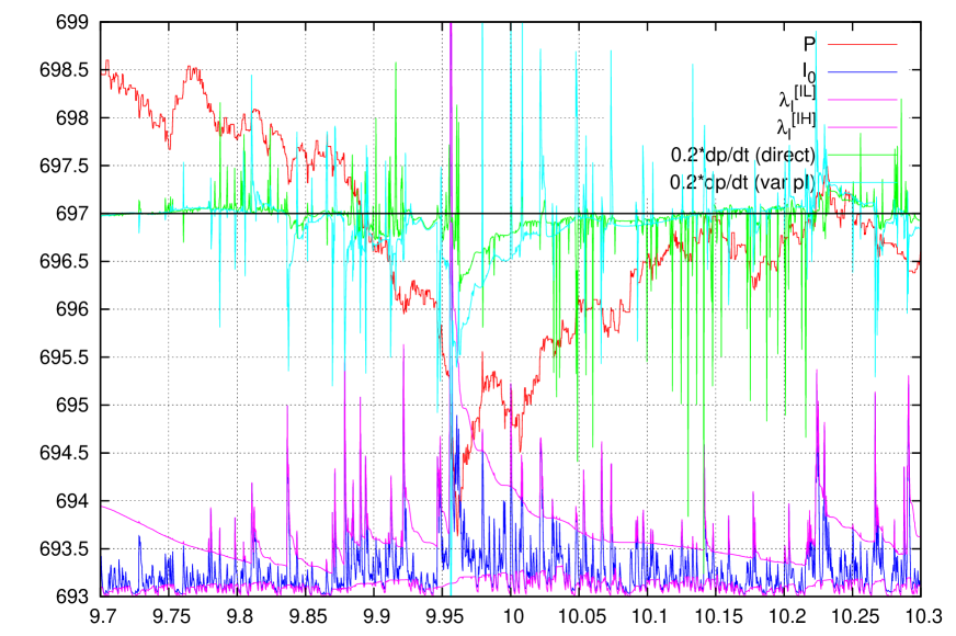
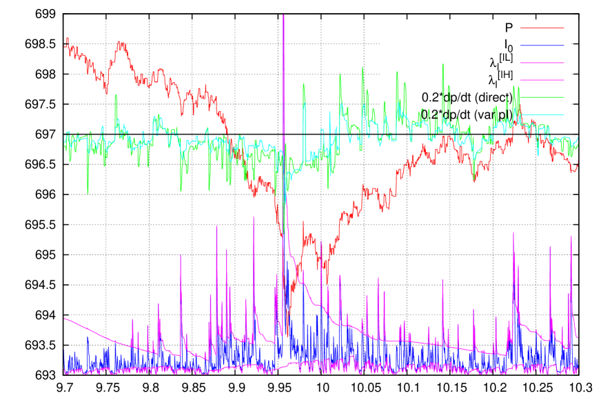
In this section we calculate generalized price impact on $\psi$ states discussed in the previous section. In Fig. 2 price change, corresponding to the state of maximal $I$ from (32) subsection V.1 and $dI/dt$ from (36) subsection V.2 are presented. In these figures

$$I_{0}=\Braket{\psi_{0}}{I}{\psi_{0}}$$ (41)

is the ‘‘$I$ now’’, calculated with the $\psi_{0}$ from (39), the $\lambda_{I}^{[IH]}=\Braket{\psi^{[IH]}_{I}}{I}{\psi^{[IH]}_{I}}$, max $I$ solution of (33), and $\lambda_{I}^{[IL]}=\Braket{\psi^{[IL]}_{I}}{I}{\psi^{[IL]}_{I}}$, the one corresponding to the minimal $\lambda_{I}$ of (33). The $dp/dt(direct)$ is calculated using (29) and $dp/dt(var\,pI)$ is calculated using (31). From these charts it is clear that:

• Boundary $dp/dt$ contribution much exceed non–boundary contribution, especially for large $I_{0}$; large $dp/dt$ typically corresponds to the boundary, i.e. large trading have just started ($\psi^{[IH]}_{I}(x)$ state is close to $\psi_{0}(x)$).

• The Eqs. (29) and (31) give similar answers only when the boundary contribution is small.

• The $dp/dt$ is typically much larger in the $\psi^{[IH]}_{I}(x)$ state, than in the $\psi^{[IH]}_{dI}(x)$ state.

This make us to conclude that:

1. The eigenfunctions of $I$ operator (33) are more important to market dynamics than the eigenfunctions of $dI/dt$ operator (37).

2. The concept of price impact is poorly applicable to market dynamics, because of large contribution of the boundary $x=x_{0}$. Because future ($x\geq x_{0}$) prediction is the goal of any market dynamics study the attributes with large boundary contribution (e.g. $dp/dt$) are poorly applicableMalyshkin and Bakhramov (2015).

3. Any consideration of infinitesimal time shifts (e.g. price impact in (29) or (31) form) is poorly applicable to market dynamics. A multi–state consideration (e.g. two different $\psi$ for enter and exit, not infinitesimal variation of some $\psi$) may be required.

4. At large $I_{0}$ the price has a singularity, same as in the quasistationary caseMalyshkin (2016). In this paper we do not use a ‘‘boundary condition $\psi(x_{0})=0$’’ as we did in Malyshkin and Bakhramov (2015), so we always have $\lambda_{I}^{[IL]}\leq I_{0}\leq\lambda_{I}^{[IH]}$, see Fig. 2. Bounded to $[0\dots 1]$ projections

   $$w^{[IL]}_{I} = \Braket{\psi_{0}}{\psi^{[IL]}_{I}}^{2}$$ (42)

   $$w^{[IH]}_{I} = \Braket{\psi_{0}}{\psi^{[IH]}_{I}}^{2}$$ (43)

   $w^{[IL]}$ and $w^{[IH]}_{I}$ are good indicators of ‘‘low’’ and ‘‘high’’ value of $I_{0}$ (also see Eq. (103) below for an alternative criteria). For a decision about ‘‘low’’ or ‘‘high’’ value of an attribute, the estimation of wavefunction projection to the state of interest is a superior approach to any classical one with a norm (i.e. $L^{2}$ or any other) and a thresholdMalyshkin (2015b).

5. This confirms our approachMalyshkin and Bakhramov (2015) to make a transition from price dynamics to execution flow and P&L dynamics. This to be considered next.

VII Impact From The Future.

While the quasistationary caseMalyshkin (2016) of dynamic equation is easy, in a non–stationary case there are several fundamental questions to be answered before considering any practical application. We start with the ‘‘infinitesimal future’’ problem: knowing the last price value, what information about future price change can be obtained.

VII.1 Open Questions (With Possible Answers)

• What ‘‘practically useful observable’’ can be directly predicted from the dynamic equationMalyshkin and Bakhramov (2015): ‘‘Future price tends to the value that maximizes the number of shares traded per unit time’’? Future value of $I_{0}$ can be predicted. The (41) gives ‘‘current’’ value of $I_{0}$, it is calculated on already executed trades. Future value of $I_{0}$ (to be calculated on yet unexecuted trades) can be estimated as $\lambda_{I}^{[IH]}$, the very important fact is that future $I_{0}$ estimator $\lambda_{I}^{[IH]}$ is calculated on already executed trades! If trading ‘‘now’’ is slow ($I_{0}$ from (41) is small), this means that at current price buyers and sellers do not match well and asset price has to move. Asset price is expected to move due to an increase in the ‘‘future’’ $I_{0}$, caused by the ‘‘future execution’’. In this sense the more slow the market now is, the more dramatic market move to be expected in the future. The ‘‘past most dramatic $I$’’, the $\lambda_{I}^{[IH]}$, can be used as a reasonably good estimator (44) of the ‘‘future dramatic $I$’’:

  $$I_{0}^{f} = \lambda_{I}^{[IH]}$$ (44)

  $$dI = I_{0}^{f}-I_{0}$$ (45)

  $$dI \geq 0$$ (46)

  Note, that similar ideology is often applied by market practitioners to asset prices or their standard deviations. This is incorrect. Experimental observationsMalyshkin (2016) show: this ideology can be applied only to execution flow $I=dV/dt$, not to the trading volume, asset price standard deviation or any other observable.

• Given the role of the execution flow $I$, what is a criteria of presence (or absense) information about the ‘‘future’’ in the ‘‘past data’’? If current $I_{0}$ from (41) is close to $\lambda_{I}^{[IH]}$, this means that we already have a ‘‘very dramatic market’’ and there is no much information about the future of this market. This is the condition of no information about the future:

  $$dI = 0$$ (47)

  But the most intriguing task would be to obtain directional information on price. The condition of no directional information about the future:

  $$\Ket{I^{f}|\psi_{0}} = \lambda\Ket{\psi_{0}}$$ (48)

  is more restrictive than (47). If the state ‘‘time is now’’, the $\psi_{0}(x)$ from (39), is an eigenfunction of $\|I^{f}\|$ operator (51), then past dynamics of $I$ has no information about the future (also note, that if $\psi_{0}(x)$ is $\|I^{f}\|$ eigenfunction, then it is $\|I\|$ eigenfuction either). The (47) is a special case of (48). Imagine extremely high volume was traded at $x=x_{0}$. Then the (33) solution, corresponding to $\lambda_{I}^{[IH]}$ is exactly the $\psi_{0}(x)$, and all other eigenfunctions ($i\neq IH$) have $\psi^{[i]}_{I}(x_{0})=0$, what immediately give the (47). Another example of (48) condition is the case when execution occurred only ‘‘now’’ ($x=x_{0}$) and in the moments of $\psi_{0}(x)$ roots, that are the nodes of Gauss–Radau quadrature built on the measure $(x_{0}-x)d\mu$, see Ref. Malyshkin and Bakhramov (2015) and computer code for calculating Gauss-type quadraturesMalyshkin (2014). One more example is, for an arbitrary $\|\widetilde{I}\|$, to consider $\|I\|=\|\widetilde{I}\|-\frac{\Ket{\widetilde{I}|\psi_{0}}\Bra{\psi_{0}|\widetilde{I}}}{\Braket{\psi_{0}}{\widetilde{I}}{\psi_{0}}}$, then this $\|I\|$ give the (48) $\|I^{f}\|$. There is one more very important situation, when information about the future cannot be obtained: assume we have a trading without execution flow fluctuations, $I=const$, then $\|I\|$ operator is degenerated (all eigenvalues are the same: $\lambda^{[i]}_{I}=I=const$), what immediately lead to both (47) and (48) being satisfied.

• While the $I=dV/dt$ dynamics is more or less understood, how can it be converted to a price dynamics? This is the most difficult problem. The relation between $p$ and $I$ is the fundamential question of market dynamics. We started this discussion in Malyshkin (2016), and have shown experimentally, that execution flow affect price much stronger (dynamic impact), than traded volume (regular impact). We also noticed there, that $p$ and $I$ often reach an extremum in the same $\psi$ state, i.e. their operators have the same eigenfunctions. Introduce dynamic impact approximation assuming asset price is affected only by the execution flow $I$, not by the volume traded:

  $$p = p(I)$$ (49)

  If (49) holds then $p$ and $I$ have the same tipping points, the behaviour we experimentally observed in Ref.Malyshkin (2016). More generally, if price is only a function of $I$ then corresponding $\|p\|$ and $\|I\|$ operators to have the same eigenfunctions, the behaviour we observedMalyshkin (2016) for the states with high $I$. We already estimated (44) future value of $I_{0}$ as $\lambda_{I}^{[IH]}$ and can build $\|I^{f}\|$ operator (51), having $dI$ contribution ‘‘from the future’’ (45). Then future value of price can be estimated considering the $\|p^{m}I^{f}\|$ operator (54), on eigenstates already found for $\|I^{f}\|$ operator (52). The price is secondary to the liquidity flow, but their common eigenfunctions allows to use future value of $I$ to calculate future value of $p$.

VII.2 Open Questions (Without Answers)

• What is the role of infinitesimal time–shift operator, available in some bases, e.g. (6) and (13)? It is very seductive to use infinitesimal time–shift operator to define a Lagrange functional (combining price volatility and execution rate), build an action $\cal S$ (like other dynamic theories do), then try to minimize $\cal S$ to build a theory combining both trend following (due to execution flow) and price reverse (due to price volatility)Malyshkin and Bakhramov (2015). Despite all our effort we failed with this plan. Even first order infinitesimal time–shift give the results similar to price impact of Section VI above. Typical for other dynamic theories second order infinitesimal time–shifts give an answer with even larger boundary $x=x_{0}$ contribution, thus having little predictive power. This make us to conclude that infinitesimal time–shifts are not very perspective for market dynamics and finite variations to be considered instead.

• What is the role of $dp/dt$ in the dynamic equation, especially, whether price volatility can be expressed through the $(dp/dt)^{2}$ term Malyshkin and Bakhramov (2015)? As we already emphaised several times above ‘‘the price is secondary to liquidity flow’’, the $dp/dt$ spikes are just a consequency of liquidity fluctuations, the charts of Section VI above seems to prove this. But this statement results in ‘‘future price does not depened on past prices’’, what make our theory too provocative, e.g. it predicts that all theories of ‘‘trend following’’ or ‘‘reverse to the mean’’ based only on price trends are invalid.

• What is the role of basis minimal and maximal time scale (how to determine $n$ and $\tau$)? If we assume that the $\Braket{Q_{j}}{f}{Q_{k}}$ matrix has all the information about $f$, then we can easily calculate the values, that cannot be directly calculated from a sampleMalyshkin and Bakhramov (2015). For example price volatility matrix in the form $(dp/dt)^{2}$, that cannot be calculated directly from sample, can be expressed through calculatable directly from sample $dp/dt$ matrix using $f=g=dp/dt$:

  $$\Braket{Q_{j}}{fg}{Q_{k}} = \sum\limits_{l,m=0}^{n-1}\Braket{Q_{j}}{f}{Q_{l}}\left(G^{-1}\right)_{lm}\Braket{Q_{m}}{g}{Q_{k}}$$ (50)

  Numerical experiment have shown this approach is not a very successful one. One can also try to compare the $\|pI\|$ matrix calculated directly $\Braket{Q_{j}}{pI}{Q_{k}}$ and Hermitian part of (50) calculated with $f=p$ and $g=I$. The $\tau$ determines a ‘‘base’’ time scale, $n$ determines the time–scale variation. While this approach is a great advance from ‘‘moving average’’–type of approaches with a single predefined time–scale (corresponds to $n=1$), now we automatically select the state out of $n$ eigenfunctions with their own time–scales (in practice $n\leq 15$), we still do not have a formal way to select proper $n$ and $\tau$.

VII.3 Impact From The Future Operator.

As we stated above maximal (33) eigenvalue, the $\lambda_{I}^{[IH]}$, can serve as an estimator of future $I_{0}$. Then execution flow operator with an impact from the future is:

$$\|I^{f}\| = \|I\|+\Ket{\psi_{0}}dI\Bra{\psi_{0}}$$ (51)

The term $\Ket{\psi_{0}}dI\Bra{\psi_{0}}$ is proportional to the execution flow of not yet executed trades $dI$ from (45); we now have $\Braket{\psi_{0}}{I^{f}}{\psi_{0}}=I_{0}^{f}$ and $\Braket{\psi_{0}}{I}{\psi_{0}}=I_{0}$. To find future equilibrium wavefunction, according to dynamic equation, eigenvalues problem for $\|I^{f}\|$ operator needs to be solved

$$\Ket{I^{f}|\psi_{I^{f}}^{[i]}} = \lambda_{I^{f}}^{[i]}\Ket{\psi_{I^{f}}^{[i]}}$$ (52)

the Eq. (52) is the same as the Eq. (33), but with the $\|I^{f}\|$ operator from (51) instead of $\|I\|$ operator in (33). Eigenvalue selection in (33) was easy, it was the state with the maximal $\lambda_{I}^{[i]}$, according to our dynamic equation (32), from where we received the (44). But for (52) the answer is not so trivial. As we demonstrated in Malyshkin (2016), asset price is much more sensitive to execution rate $I=dV/dt$, rather than to trading volume $V$, thus in dynamic impact approximation (49) the contribution of $\Ket{\psi^{[i]}_{I^{f}}}$ state to future price changes is proportional to the flow of not yet executed trades $\Braket{\psi^{[i]}_{I^{f}}}{\psi_{0}}^{2}dI$. For this reason we are going to keep all eigenfunctions of (52) problem. The $\Ket{\psi^{[i]}_{I^{f}}}$ is $\|I^{f}\|$ operator eigenfunction (52), thus first order variation (53) is equal to zero for arbitrary $\Ket{\delta\psi}$.

$$\frac{1}{2}\delta\frac{\Braket{\psi^{[i]}_{I^{f}}}{I^{f}}{\psi^{[i]}_{I^{f}}}}{\Braket{\psi^{[i]}_{I^{f}}}{\psi^{[i]}_{I^{f}}}}=\Braket{\psi^{[i]}_{I^{f}}}{I^{f}}{\delta\psi}-\Braket{\psi^{[i]}_{I^{f}}}{I^{f}}{\psi^{[i]}_{I^{f}}}\Braket{\psi^{[i]}_{I^{f}}}{\delta\psi} = 0$$ (53)

The $\|p^{m}I^{f}\|$ operator (for practical applications it is more convenient to consider operator $p^{m}I$ instead of $p^{m}$) with an impact from the future is:

$$\|p^{m}I^{f}\| = \|p^{m}I\|+\Ket{\psi_{0}}P^{fm}dI\Bra{\psi_{0}}$$ (54)

$$P^{fm} = \left(P^{last}\right)^{m}$$ (55)

The term $\Ket{\psi_{0}}P^{fm}dI\Bra{\psi_{0}}$ for $m=1$ is proportional to execution capital flow of not yet executed trades at unknown future price $P^{f1}$ with known future execution rate contribution $dI$ from (45). ‘‘The last price as $P^{f}$ estimator (55)’’ is the simplest estimation, meaning the best estimation of future price is current value. In equilibrium the $\|p\|$ and $\|I^{f}\|$ to have the same eigenfunctions $\Ket{\psi^{[i]}_{I^{f}}}$, at least for the states with a high $\lambda^{[i]}_{I^{f}}$, so the most promissing idea is to consider $\|p^{m}I^{f}\|$ operator on eigenstates of $\|I^{f}\|$ and $\|\frac{d}{dt}I^{f}\|$.

VII.4 Equilibrium Price in Naïve Dynamic Impact Approximation

In pure dynamic impact approximation formal answer for future equilibrium price can be obtained. This answer is not a very practical, so we would call it Naïve Dynamic Impact Approximation, but it is worth considering to compare it with the answer from our previous workMalyshkin and Bakhramov (2015).

Figure 3: The AAPL stock price on September, 20, 2012. $P^{[IH]}$ (61) (pink), $P^{f}$ (60) (green), and $\Upsilon$ (59) (shifted to 694 level to fit the chart). Calculated in Shifted Legendre basis with $n=7$ and $\tau$=128sec.

Future equilibrium price $P^{f}$ enter impact from the future operator (54) from which $P_{0}$ is calculated as:

$$P_{0}=\frac{\Braket{\psi_{0}}{pI^{f}}{\psi_{0}}}{\Braket{\psi_{0}}{I^{f}}{\psi_{0}}}$$ (56)

Now, assume $\|pI^{f}\|$ and $\|I^{f}\|$ are diagonal in the same basis, the solution of (52). Expanding $\Ket{\psi_{0}}=\sum_{i=0}^{n-1}\Braket{\psi_{0}}{\psi_{I^{f}}^{[i]}}\Ket{\psi_{I^{f}}^{[i]}}$ and assuming all off diagonal ($i\neq j$) matrix $\|pI^{f}\|$ elements are zero: $\Braket{\psi_{I^{f}}^{[i]}}{pI}{\psi_{I^{f}}^{[j]}}=0$, same as we have for $\|I^{f}\|$ in (52). Then the $P_{0}$ can be estimated only from diagonal elements of $\|pI^{f}\|$:

$$P_{0}=\sum\limits_{i=0}^{n-1}\frac{\Braket{\psi^{[i]}_{I^{f}}}{pI^{f}}{\psi^{[i]}_{I^{f}}}}{\lambda_{I^{f}}^{[i]}}\Braket{\psi_{0}}{\psi^{[i]}_{I^{f}}}^{2}$$ (57)

Then (56) and (57) with (54) give the solution for $P^{f}$:

$$\frac{\Braket{\psi_{0}}{pI^{f}}{\psi_{0}}}{I_{0}^{f}} = \sum\limits_{i=0}^{n-1}\frac{\Braket{\psi^{[i]}_{I^{f}}}{pI^{f}}{\psi^{[i]}_{I^{f}}}}{\lambda_{I^{f}}^{[i]}}\Braket{\psi_{0}}{\psi^{[i]}_{I^{f}}}^{2}$$ (58)

$$\Upsilon = 1-\sum\limits_{i=0}^{n-1}\Braket{\psi_{0}}{\psi^{[i]}_{I^{f}}}^{4}\frac{I_{0}^{f}}{\lambda_{I^{f}}^{[i]}}$$ (59)

$$P^{f} = \frac{1}{\Upsilon dI}\left(-\Braket{\psi_{0}}{pI}{\psi_{0}}+\sum\limits_{i=0}^{n-1}\Braket{\psi^{[i]}_{I^{f}}}{pI}{\psi^{[i]}_{I^{f}}}\Braket{\psi_{0}}{\psi^{[i]}_{I^{f}}}^{2}\frac{I_{0}^{f}}{\lambda_{I^{f}}^{[i]}}\right)$$ (60)

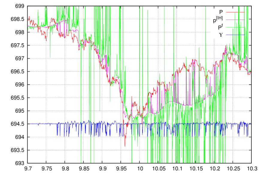
Conceptually (but not practically) the (60) directional answer is a giant step forward from our previous workMalyshkin and Bakhramov (2015), where the best directional estimator was the difference between last price and the price $P^{[IH]}$, corresponding to the state of maximal $I$ on past sample, the (30) calculated on $\Ket{\psi^{[IH]}_{I}}$ state (34):

$$P^{[IH]} = \frac{\Braket{\psi^{[IH]}_{I}}{pI}{\psi^{[IH]}_{I}}}{\lambda_{I}^{[IH]}}$$ (61)

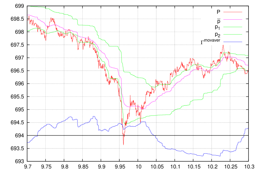
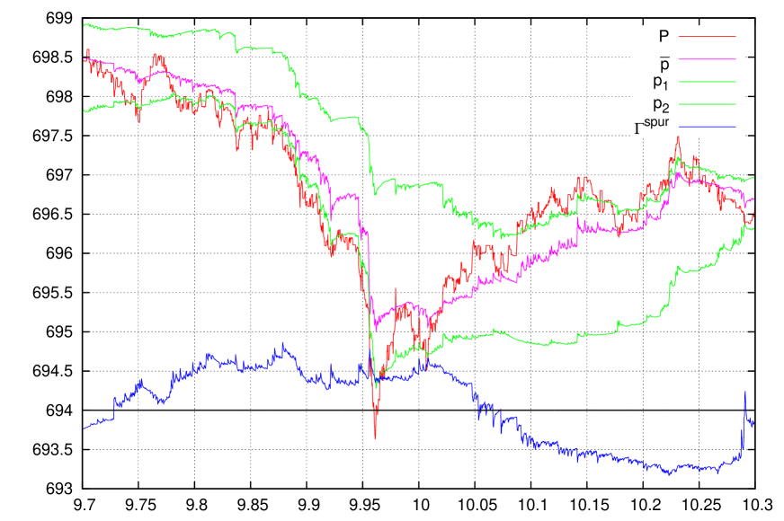
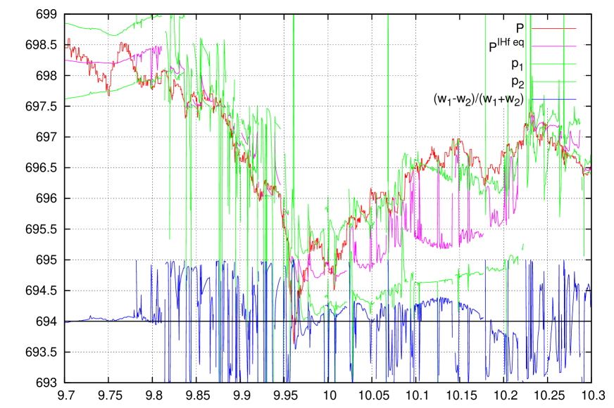
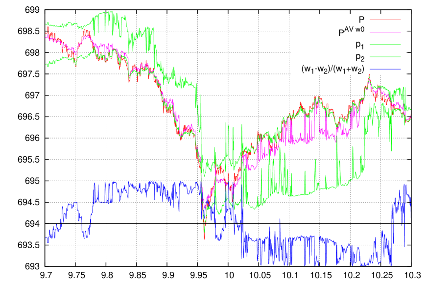
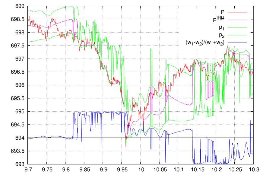
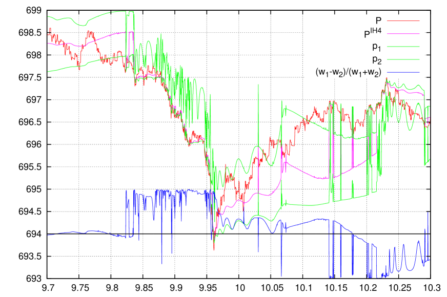
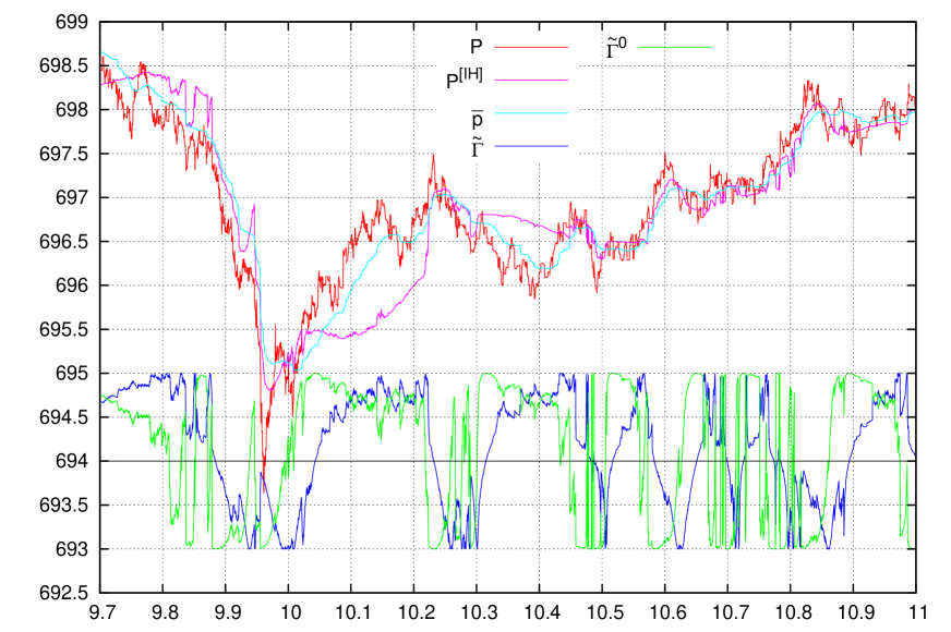
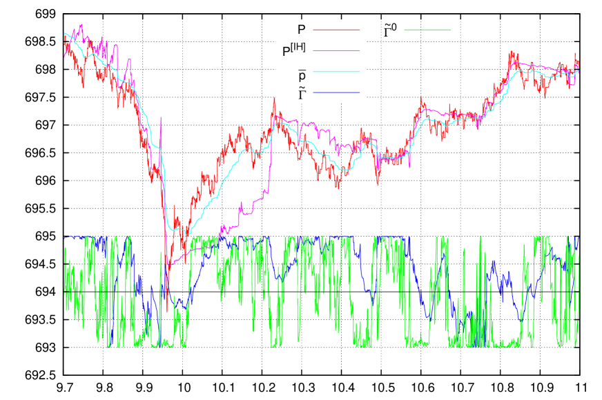
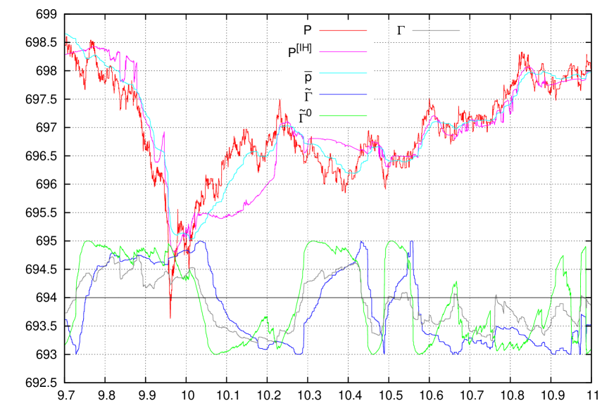
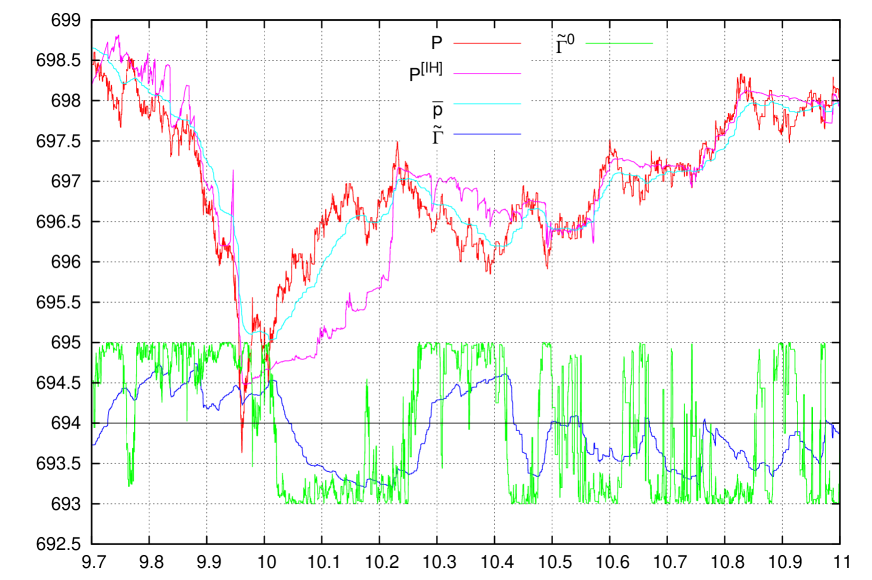
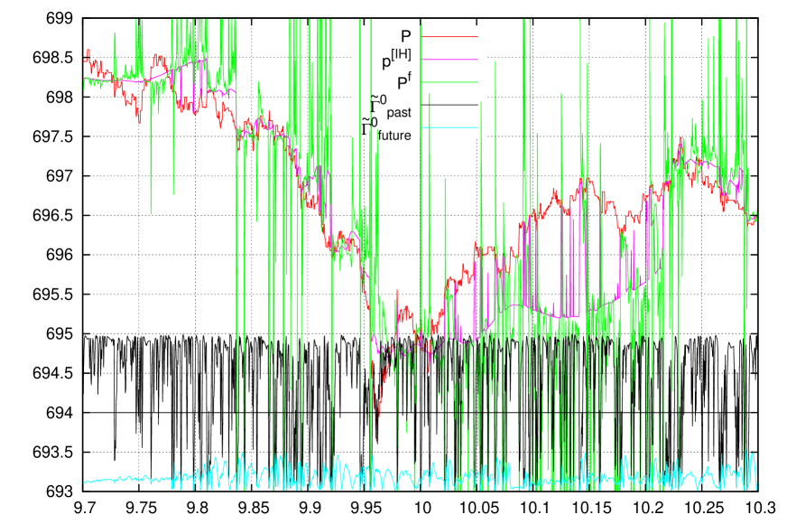
This Ref. Malyshkin and Bakhramov (2015) answer is asset price averaged on past sample with always positive weight $\left(\psi^{[IH]}_{I}(x)\right)^{2}Id\mu(x)$; no explicit information about the future is used in this averaging. The (60) answer is very different: it directly incorporates information about not yet executed trades from the future using $dI$ and $\Ket{\psi^{[i]}_{I^{f}}}$ obtained from (44) assumption about $I_{0}^{f}$. The $\Upsilon$ from (59) formally define the degree of degeneracy, how much directional information can be obtained from the sample, it is zero when $\Ket{\psi_{0}}$ is (52) eigenvector, condition (48). Future volatility prediction is easy, for example (42) and (43) projections can be used to estimate whether current $I_{0}$ (41) is ‘‘low’’ or ‘‘high’’, then use (45). Future directional prediction is much more complicated, the (60) is the simplest (naïve) directional answer that can be obtained. In Fig. 3 the $P^{[IH]}$ (61), $P^{f}$ (60), and $\Upsilon$ (59) are presented. The degeneracy $\Upsilon$ typically has a value $1/2$, but going to $0$ at times of high $I_{0}$, what correspond to (48) condition. In Malyshkin and Bakhramov (2015) the difference between last price and $P^{[IH]}$ was used as a directional estimator. If $P^{f}$ is used instead, the result, as one see from Fig. 3 is very similar (sign does not change), but, as expected, $P^{f}$ is not close to last price at high $I_{0}$. The (60) is asset price averaged on past sample, but, in contrast with (61), with the weight, which is not always positive. This lead to a divergence in $P^{f}$ (especially at low $\Upsilon$ and/or small $dI$). This divergence typically does not change the $P^{last}-P^{f}$ sign. Overall the (60) seems to be a marginal improvement over our old answer (61), this is why we call (60) naïve answer. For computer implementation see the PnLdIDSk.Pf_from_pt_true_pi for $P^{f}$ and PnLdIDSk.deg_from_pt_true_pi for $\Upsilon$. Computer code structure is described in appendix G.3.

VIII Selection of Time–Scale, Then Determine Price Distribution Asymmetry From Quadrature. Trend–Following vs. Reverse to the Mean

Equilibrium price estimation, let it be (60) of previous section or (61) of our previous workMalyshkin and Bakhramov (2015), and using the difference between $P^{last}$ and calculated price as directional indicator, typically does not give a satisfactory results, as price is secondary concept to market dynamics. The characteristics, describing the P&L distribution should be considered instead.

Let us start with the simplest problem of price distribution. As we discussed in Section III a measure is defined by a wavefunction $\psi(x)$, the measure is $\psi^{2}(x)d\mu$, then price moments $\pi_{m}$, $m=0,1,2,3$ are:

$$\pi_{m} = \Braket{\psi}{p^{m}I}{\psi}$$ (62)

(similar expression without $I$ can be used $\Braket{\psi}{p^{m}}{\psi}$, but (62) choice is better in applications). The (62) expression selects the time scale based on $\psi(x)$ choice. This way (via $\psi(x)$) the (45) information about future $I$ can be incorporated. Different $\psi(x)$ choices are considered below. For now assume, that some $\psi(x)$ is chosen and the goal is to estimate price distribution on the measure generated by this $\psi(x)$ . The standard approach is to consider price average, standard deviation and skewness. In the Appendix C of Ref. Malyshkin and Bakhramov (2015) modified skewness estimator was introduced. The $\pi_{m}$ moments describe how the price is distributed at times of the support of the measure. The skewness of the distribution is typically used for estimation of future price direction. However, a much better, than a regular skewness, answer can be obtained. The idea is to build two–point Gauss quadrature out of $\pi_{m}$, $m=0,1,2,3$ moments then consider quadrature weights asymmetry (single–point Gauss quadrature require two moments $\pi_{0}$ and $\pi_{1}$ to calculate and give price average as the node: $p_{1}=\pi_{1}/\pi_{0}$, the weight $w_{1}=\pi_{0}$). It is very important, that besides weights, two–point quadrature nodes can be used to determine threshold levels. The two nodes $\lambda_{p}^{[s]}$ are generalized eigenvalue problem solution:

$$\left(\begin{array}[]{ll}\pi_{1}&\pi_{2}\\ \pi_{2}&\pi_{3}\end{array}\right)\left(\begin{array}[]{l}\alpha_{0}^{[s]}\\ \alpha_{1}^{[s]}\end{array}\right) = \lambda_{p}^{[s]}\left(\begin{array}[]{ll}\pi_{0}&\pi_{1}\\ \pi_{1}&\pi_{2}\end{array}\right)\left(\begin{array}[]{l}\alpha_{0}^{[s]}\\ \alpha_{1}^{[s]}\end{array}\right)$$ (71)

$$p_{\{1,2\}} = \lambda_{p}^{[\{1,2\}]}$$ (72)

$$w_{\{1,2\}} = \frac{1}{\left(\alpha_{0}^{[\{1,2\}]}+\lambda_{p}^{[\{1,2\}]}\alpha_{1}^{[\{1,2\}]}\right)^{2}}$$ (73)

$$\Gamma = \frac{w_{1}-w_{2}}{w_{1}+w_{2}}=\frac{2\overline{p}-p_{1}-p_{2}}{p_{1}-p_{2}}$$ (74)

The quadrature nodes $p_{\{1,2\}}$ are the eigenvalues (72) (we assume $p_{1}<p_{2}$), and the quadrature weights $w_{\{1,2\}}$ are expresses via the eigenfunction (73), for numerical calculation see the class com/polytechnik/utils/Skewness.java. Note that defined in (74) skewness $\Gamma$ is similar in concept to the ‘‘signed volume’’ (the difference between market–sell matched limit–buy and market–buy matched limit–sell orders). As we emphasized earlierMalyshkin and Bakhramov (2016), regular signed volume concept is not a practical one. Important, that (74) definition allows us to obtain volume difference from trades history only, no matching type knowledge is required. See alternative formulas for (74) in the Appendix C of Ref. Malyshkin and Bakhramov (2015) to obtain (72) and (73) by minimizing over the $p_{\{1,2\}}$ nodes the expression:

$$L^{4}volatility = \Braket{\psi}{(p-p_{1})^{2}(p-p_{2})^{2}I}{\psi}\to\min$$ (75)

The (75) is the definition of $L^{4}$ volatility, minimization of which give the $p_{\{1,2\}}$ nodes (72). Compare it to well known ‘‘minimizing volatility as standard deviation over the $\overline{p}$’’:

$$L^{2}volatility = \Braket{\psi}{(p-\overline{p})^{2}I}{\psi}\to\min$$ (76)

that gives the (81) expression for the average price $\overline{p}$ (single node Gauss quadrature) and to kurtosis calculation as $\Braket{\psi}{(p-\overline{p})^{4}I}{\psi}$. For two variables $p$ and $r$ a $L^{4}covariation$, correlating (71) eigenfunction (they are proportional to Lagrange interpolating polynomials) for $p$ and $r$ quadratures can be introduced, see Appendix B below for calculations.

Two point Gauss quadrature give exact integration answer for integration of a polynomial of degree 3 or less ($n$ point quadrature is exact for a polynomial of degree $2n-1$ or less). Familiar average, standard deviation and skewness can be expressed by averaging at $p_{1}$ with the weight $w_{1}$ and at $p_{2}$ with the weight $w_{2}$:

$$\pi_{0} = w_{1}+w_{2}$$ (77)

$$\pi_{1} = p_{1}w_{1}+p_{2}w_{2}$$ (78)

$$\pi_{2} = p^{2}_{1}w_{1}+p_{2}^{2}w_{2}$$ (79)

$$\pi_{3} = p_{1}^{3}w_{1}+p_{2}^{3}w_{2}$$ (80)

$$\overline{p} = \frac{\pi_{1}}{\pi_{0}}=p_{1}\frac{w_{1}}{w_{1}+w_{2}}+p_{2}\frac{w_{2}}{w_{1}+w_{2}}$$ (81)

$$\overline{\left(p-\overline{p}\right)^{2}} = (p_{1}-\overline{p})^{2}\frac{w_{1}}{w_{1}+w_{2}}+(p_{2}-\overline{p})^{2}\frac{w_{2}}{w_{1}+w_{2}}$$ (82)

$$\overline{\left(p-\overline{p}\right)^{3}} = (p_{1}-\overline{p})^{3}\frac{w_{1}}{w_{1}+w_{2}}+(p_{2}-\overline{p})^{3}\frac{w_{2}}{w_{1}+w_{2}}$$ (83)

The distribution itself can now be considered as two–mode distribution: trading at $p_{1}$ with the weight $w_{1}$ and trading at $p_{2}$ with the weight $w_{2}$. This gives huge advantage: an opportunity to implement ‘‘follow the trend’’ type of strategy. For a single–point Gauss quadrature the only node is price average $\overline{p}$ and only strategy available is ‘‘reverse–to-the–average’’ type of strategy (average price as an attractor). For two–point Gauss quadrature one can implement a ‘‘follow the trend’’ type of strategy (average price as a repeller, $p_{\{1,2\}}$ as the attractors), in a most simplistic way it is: ‘‘Open Short when $p_{1}<P^{last}<\overline{p}$; Open Long when $\overline{p}<P^{last}<p_{2}$; combine with weights asymmetry’’. The two new price levels: $p_{1}$ and $p_{2}$ allow to have a completely new look to trend–following trading: if $\pi_{m}$ are moving–average moments, then the $p_{1}$ and $p_{2}$ are much better thresholds than often used $\overline{p}\pm\sigma$, because they include the skewness of price distribution, the thresholds are now different for up and down moves, according to the distribution skewness. This approach is much more generic, than this simple demonstration. The key components of it are:

• Find the $\psi$ of interest. Several choices of $\psi$ are considered below. As we emphasized above the most interesting $\psi$ is the one maximizing the $\|I^{f}\|$ operator according to the dynamic equation. However, other $\psi$ choices can be also considered, at least for the purpose of the demonstration of the technique.

• Given $\psi$ obtain the measure $\psi^{2}(x)d\mu$ to calculate price moments $\pi_{m}$ from (62) Then Gauss quadrature nodes $p_{\{1,2\}}$ and weights $w_{\{1,2\}}$ to be obtained. This quadrature determines the distribution of price in the $\psi$ state. One can try to obtain some directional information on price from this distribution (e.g. skewness estimation (74)). Note, that when using (54) operators, with an impact from the future term, future price $P^{f}$ is required to calculate the moments, ‘‘the last price as $P^{f}$ estimator (55)’’ is a very crude approximation. While future price $P^{f}$ is unknown, all the calculations above can be reperated using $P^{f}$ as a parameter, see Appendix D below where the dependendce of $\Gamma(P^{f})$ on $P^{f}$ is obtained (161).

• In addition, some other value $r$ (e.g. market index, etc.) can be considered and cross–correlation of Appendix B below can be performed.

IX Demonstration of price–distribution estimation from two–point Gauss quadrature built for a measure of interest

Let us demonstrate the technique of building two–point Gauss quadrature out of $\pi_{m}$ moments (62) calculated for a number of $\psi$ choices.

IX.1 Measure: Moving Average and Moving Average –Like

Figure 4: The AAPL stock price on September, 20, 2012. Top: Demonstration of Gauss quadrature calculation with moving average (84) moments, $\overline{p}=\pi_{1}/\pi_{0}$ – exponential moving average with $\tau$=128sec, $p_{1}$, $p_{2}$ – quadrature nodes calculated according to (71), and modified skewness (74) $\Gamma$ (shifted to 694 level to fit the chart). Bottom: same thing with (85) mixed state moments.

The most simple example is moving average–type of measure (corresponds to $\psi(x)=1$, also assume here, that there is no impact from the future: $dI=0$). Calculate the moments:

$$\pi_{m} = \Braket{p^{m}I}$$ (84)

Then $\overline{p}_{\tau}=\pi_{1}/\pi_{0}=p_{1}\frac{w_{1}}{w_{1}+w_{2}}+p_{2}\frac{w_{2}}{w_{1}+w_{2}}$ is regular exponential moving average. Gauss quadrature nodes $p_{\{1,2\}}$ and weights $w_{\{1,2\}}$ are calculated according to (71), and $\Gamma$ from (74). These values are presented in Fig. 4. Even in this non–practical example (because of fixed time–scale $\tau$) we clearly see an asymmetry between $\overline{p}_{\tau}$ and $p_{\{1,2\}}$. Median estimator $(p_{1}+p_{2})/2$ is equal to average $\overline{p}_{\tau}$ only in the case of zero skewness. We also see good skewness correlation with price trend, but, as for any model with a fixed time–scale, there is fixed time delay between price trend change and skewness change. However, the asymmetry between $\overline{p}$ and $p_{\{1,2\}}$ is a remarkable feature that may be incorporated to a trading model, because three levels now allow to implement a ‘‘follow–the–trend’’ type of strategy.

There is a characteristics, that is very similar to exponential moving average, but described by a density–matrix state, it cannot be reduced to a state of some $\Ket{\psi}$. In its simplistic form the $\pi_{m}$ moments are matrix spur:

$$\pi_{m} = \sum\limits_{i=0}^{n-1}\Braket{\psi^{[i]}_{I}}{p^{m}I}{\psi^{[i]}_{I}}$$ (85)

These are different from (96) in Section IX.5 below in absence of the impact from the future term, $dI=0$. (Note, that (85) is invariant with respect to basis transform, also seeMalyshkin and Bakhramov (2015) Appendix E of the expression in a non–orthogonal basis: $\pi_{m}=\sum\limits_{j,k=0}^{n-1}(G^{-1})_{jk}\Braket{Q_{k}}{p^{m}I}{Q_{j}}$). The result is presented in Fig. 4 bottom. It is very similar to moving average result, as expected. These two kind of ‘‘moving average’’: with (84) ‘‘pure state’’ and (85) ‘‘mixed state’’ moments, demonstrate wavefunction and density–matrix approaches. In this section we specifically chose the situation, when both approaches give very similar result.

IX.2 Measure: The Period of Maximal Future $I$

Figure 5: The AAPL stock price on September, 20, 2012. Demonstration of Gauss quadrature calculation with the state (moments $\pi_{m}$ from (86)),corresponding to maximal $\|I^{f}\|$ (top) and (moments $\pi_{m}$ from (87)), maximal $\|I\|$ (bottom). The prices and skewness are presented as in Fig. 4 above.

Consider the periods of maximal future $I$. The ‘‘future’’ time scale is determined by the future state $\Ket{\psi^{[IH]}_{I^{f}}}$, the eigenfunction of (51) operator, the (52) solution, corresponding to maximal eigenvalue $\lambda_{I^{f}}^{[IH]}$. The $\|p^{m}I^{f}\|$ operators and $\pi_{m}$ moments for $m=0,1,2,3$ are:

$$\pi_{m} = \Braket{\psi^{[IH]}_{I^{f}}}{p^{m}I^{f}}{\psi^{[IH]}_{I^{f}}}$$ (86)

To practically calculate the $\pi_{m}$ — the value of $dI$ is known (45) and last price $P^{last}$ can be used as $P^{fm}$ estimator (55). The result is presented in Fig. 5 top.

Then compare the results with the $\Ket{\psi^{[IH]}_{I}}$ choice for $\psi(x)$, not having an impact from the future contribution, when the moments

$$\pi_{m} = \Braket{\psi^{[IH]}_{I}}{p^{m}I}{\psi^{[IH]}_{I}}$$ (87)

are calculated in the $\Ket{\psi^{[IH]}_{I}}$ state, the (33) solution (without an impact from the future term $P^{f}$ estimator is not required). The result is presented in Fig. 5 bottom. One can see the importance of the impact from the future term, however in this simplistic form price skewness has some issues as market directional indicator.

IX.3 Measure: The Period of Maximal Future $I$ with equilibrium $P^{f}$ estimator

Figure 6: The AAPL stock price on September, 20, 2012. Demonstration of Gauss quadrature calculation with the state (moments $\pi_{m}$ from (91)), corresponding to maximal $\|I^{f}\|$ The prices and skewness are presented as in Fig. 4 above.

While (86) moments from previous section are very promising they have one conceptional weakness: using $P^{last}$ as $P^{f}$ estimator (55). Consider $\|p^{m}I^{f}\|$ operator (54) with an impact from the future. The idea is to modify (55) estimator to obtain some ‘‘equilibrium’’ value of $P^{fm}$.

As we discussed in Section VII.3 the $\|I^{f}\|$ and the $\|p^{m}I^{f}\|$ operators to have the same eigenfunctions, thus first order variation should be equal to zero for arbitrary $\Ket{\delta\psi}$, same as for $\|I^{f}\|$ in (53):

$$\Braket{\psi^{[i]}_{I^{f}}}{p^{m}I^{f}}{\delta\psi}-\Braket{\psi^{[i]}_{I^{f}}}{p^{m}I^{f}}{\psi^{[i]}_{I^{f}}}\Braket{\psi^{[i]}_{I^{f}}}{\delta\psi} = 0$$ (88)

The (53) holds for arbitrary $\Ket{\delta\psi}$, but for variations (88) only a single parameter $P^{fm}$ is available, thus zero–sensitivity condition can be satisfied only for a single $\Ket{\delta\psi}$, besides trivial $\Ket{\delta\psi}=\Ket{\psi^{[i]}_{I^{f}}}$. There are a number of options for $\Ket{\delta\psi}$ variation to consider:

• $\Ket{D(\psi^{[i]}_{I^{f}})}:$ Zero price impact (31) (zero sensitivity to infinitesimal time–shift).

• $\Ket{\psi_{0}}:$ Zero sensitivity to $\Ket{\psi^{[i]}_{I^{f}}}\to\Ket{\psi_{0}}$ transition.

• $\Ket{\psi^{[IH]}_{I}}:$ Zero sensitivity to $\Ket{\psi^{[i]}_{I^{f}}}\to\Ket{\psi^{[IH]}_{I}}$ transition.

among many others.

The $P^{[i]\,fm}dI$ estimation, corresponding to (88) equilibrium of (54) operator on $\Ket{\psi^{[i]}_{I^{f}}}$ state with $\Ket{\delta\psi}$ variation is:

$$P^{[i]\,fm}dI = \frac{\Braket{\psi^{[i]}_{I^{f}}}{p^{m}I}{\psi^{[i]}_{I^{f}}}-\frac{\Braket{\psi^{[i]}_{I^{f}}}{p^{m}I}{\delta\psi}}{\Braket{\psi^{[i]}_{I^{f}}}{\delta\psi}}}{\frac{\Braket{\psi^{[i]}_{I^{f}}}{\psi_{0}}\Braket{\psi_{0}}{\delta\psi}}{\Braket{\psi^{[i]}_{I^{f}}}{\delta\psi}}-\Braket{\psi^{[i]}_{I^{f}}}{\psi_{0}}^{2}}$$ (89)

For the most interesting case $\Ket{\delta\psi}=\Ket{\psi_{0}}$ obtain:

$$P^{[i]\,fm}dI = \frac{\Braket{\psi^{[i]}_{I^{f}}}{p^{m}I}{\psi^{[i]}_{I^{f}}}-\frac{\Braket{\psi^{[i]}_{I^{f}}}{p^{m}I}{\psi_{0}}}{\Braket{\psi^{[i]}_{I^{f}}}{\psi_{0}}}}{1-\Braket{\psi^{[i]}_{I^{f}}}{\psi_{0}}^{2}}$$ (90)

Then for the state with the maximal $\lambda_{I^{f}}^{[i]}$ ($i=IH$):

$$\pi_{m} = \frac{\Braket{\psi^{[IH]}_{I^{f}}}{p^{m}I}{\psi^{[IH]}_{I^{f}}}-\Braket{\psi^{[IH]}_{I^{f}}}{p^{m}I}{\psi_{0}}\Braket{\psi^{[IH]}_{I^{f}}}{\psi_{0}}}{1-\Braket{\psi^{[IH]}_{I^{f}}}{\psi_{0}}^{2}}$$ (91)

Obtained $\pi_{m}$ have a term $\Braket{\psi^{[IH]}_{I^{f}}}{p^{m}I}{\psi_{0}}$ added to have zero variation (88). In Fig. 6 corresponding chart is presented. First, what is clearly seen is that Gauss quadrature does not always exist. This is because (90) may not always give a positive standard deviation. However, the formulae for the first moment is actually similar to naïve dynamic impact approximation of Section VII.4 and demonstrate an approach of searching a $\Ket{\delta\psi}$ to variate (88). Despite all our effort we did not achieve much success with this search of $\Ket{\delta\psi}$, and now think that (88) variation can be a good option only for the first moment, what can give only a equilibrium price (first moment).

IX.4 Measure: The Period After Maximal Future $I$

Figure 7: The AAPL stock price on September, 20, 2012. Demonstration of Gauss quadrature calculation with the state (moments $\pi_{m}$ from (93) with the impact from the future), corresponding to the state of the maximal $\|I^{f}\|$ (top) and (moments $\pi_{m}$ from (93), without an impact from the future), corresponding to the state of the maximal $\|I\|$ (bottom). The prices and skewness are presented as in Fig. 4 above.

The $\pi_{m}$ choices (86) and (87) are considering price distribution during the spikes for the future and for the past $I$ respectively. It is very interesting to consider the time period after a spike in $I$. Consider $V_{m}$ and $T_{m}$:

$$V_{m}(t) =\int\limits_{t}^{t_{now}}p^{m}Idt^{\prime}=\int\limits_{t}^{t_{now}}p^{m}dV^{\prime}$$ (92a)

$$T_{m}(t) =\int\limits_{t}^{t_{now}}p^{m}dt^{\prime}$$ (92b)

Here $V_{0}(t)$ is traded volume, $V_{1}(t)$ is traded capital, $V_{1}(t)/V_{0}(t)$ is volume–weighted average price, $T_{1}(t)/T_{0}(t)$ is time–weighted average price. These values are calculated for the interval between $t$ and $t_{now}$. Then for a given $\psi(x)$

$$\pi_{m} = \Braket{\psi}{V_{m}}{\psi}$$ (93)

Note, that for the measures allowing an integration by parts (i.e. the ones with infinitesimal time–shift operators such as (6) or (13)) the (93) can be interpreted as a transition from an averaging with the $\psi^{2}(x)d\mu$ weight to an averaging with the $w_{\psi}(t)dt$ weight:

$$w_{\psi}(t) = \int\limits_{-\infty}^{t}\psi^{2}(x^{\prime})\frac{d\mu^{\prime}}{dt^{\prime}}dt^{\prime}$$ (94)

$$\pi_{m} = \int\limits_{-\infty}^{t_{now}}p^{m}Iw_{\psi}(t^{\prime})dt^{\prime}$$ (95)

$w_{\psi}(t_{now})=1$ follows from the $\psi(x)$ normalizing. For (4) and (11) measures the (93) can be calculated from the $\Braket{Q_{k}p^{m}I}$ matrix elements using an integration by parts. For these measures Eqs. (93) and (95) are identical.

Consider a $\psi(x)$, defining the spikes in $I$, the $\Ket{\psi^{[IH]}_{I^{f}}}$ or $\Ket{\psi^{[IH]}_{I}}$ from the previous section. Then (93) moments give very much a ‘‘moving average with automated time–scale selection’’ measure. These averages are calculated for the period of time: between the spike in $I$ and $t_{now}$.

The results are presented in Fig. 7. They are worse than that of the previous sections, what probably manifest the importance of the execution flow $I$ dynamics over the volume $V$ dynamics. This correspond to our earlier work Malyshkin (2016), where an importance of dynamic impact was emphasized experimentally. See also the discussion below in Section XI, where the $V$– and $I$– dynamics are discussed from a different perspective.

IX.5 Measure: Density matrix mixed state of pure $\Ket{\psi^{[i]}_{I^{f}}}$ states.

Figure 8: The AAPL stock price on September, 20, 2012. Demonstration of Gauss quadrature calculation with the mixes states: moments $\pi_{m}$ from (96) (top) and moments $\pi_{m}$ from (97) (bottom). The prices and skewness are presented as in Fig. 4 above.

As we discussed in Section VII.3 above, in case of the impact from the future presence, proper eigenstate selection is not a trivial question. In the Sections IX.2 and IX.3 the state, corresponding to the maximal $I$, was considered. There are several alternatives. Consider matrix–averages (introduced in the Appendix E of Ref. Malyshkin and Bakhramov (2015), see Ref. Malyshkin (2015b) for quantum mechanics density matrix mixed state relation):

$$\pi_{m} = \sum\limits_{i=0}^{n-1}\Braket{\psi^{[i]}_{I^{f}}}{p^{m}I^{f}}{\psi^{[i]}_{I^{f}}}$$ (96)

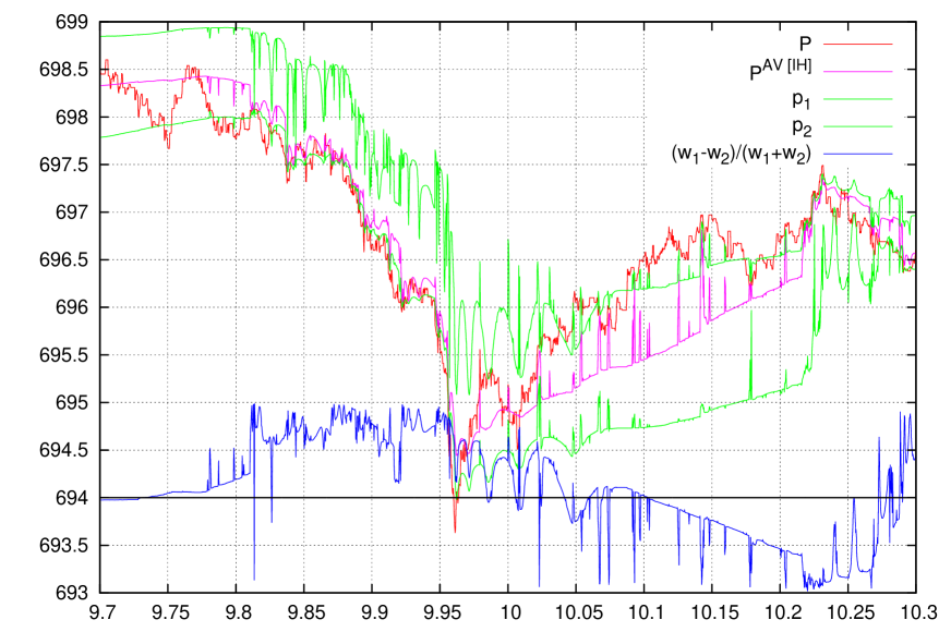
(in this section, when estimating the $\|p^{m}I^{f}\|$ matrix elements, we assume (55) $P^{fm}$ estimation for simplicity). The (96) answer is very much a moving–average type of answer (84), it is basis–invariant (a unitary transform of $\Ket{\psi^{[i]}_{I^{f}}}$ basis does not change the result) and can be considered as a density–matrix mixed stateMalyshkin (2015b) with equal contribution of each pure state.

Alternatively, a density–matrix mixed state with $\Braket{\psi^{[i]}_{I^{f}}}{\psi_{0}}^{2}$ contribution of a pure state $\Ket{\psi^{[i]}_{I^{f}}}$ can be considered:

$$\pi_{m} = \sum\limits_{i=0}^{n-1}\Braket{\psi^{[i]}_{I^{f}}}{p^{m}I^{f}}{\psi^{[i]}_{I^{f}}}\Braket{\psi^{[i]}_{I^{f}}}{\psi_{0}}^{2}$$ (97)

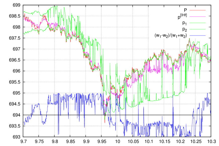
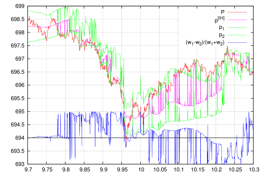
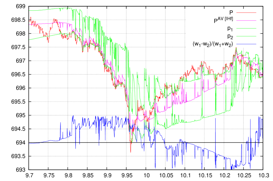
The (97) result is not basis–invariant and implicitly assume dynamic impact approximation (49) of $\|p\|$ and $\|I^{f}\|$ operators being simultaneous diagonal in the $\Ket{\psi^{[i]}_{I^{f}}}$ basis. The (97) is similar to (86), because $\|I^{f}\|$ state with the maximal $\Ket{\psi_{0}}$ projection is almost always the $\Ket{\psi^{[IH]}_{I^{f}}}$ state. The results are presented in Fig. 8. They are not much different from the Sections IX.1 and IX.2 of above. This section demonstrate that density matrix approach is a viable option for the market dynamics, but, at this stage of development, does not give much compared to wavefunction pure states.

IX.6 Measure: Combine maximal Future $I$ and minimal price volatility

Figure 9: The AAPL stock price on September, 20, 2012. Demonstration of Gauss quadrature calculation with the state corresponding to $\max\limits_{\psi}\min\limits_{p_{1},p_{2}}\Braket{\psi}{(p-p_{1})^{2}(p-p_{2})^{2}I^{f}}{\psi}$ (top) and $\max\limits_{\psi}\min\limits_{p_{1},p_{2}}\Braket{\psi}{(p-p_{1})^{2}(p-p_{2})^{2}I}{\psi}$ (bottom). The prices and skewness are presented as in Fig. 4 above.

The approach of section IX.2 where $\psi$ corresponding to the maximum of $\Braket{\psi}{I^{f}}{\psi}/\Braket{\psi}{\psi}\to\max$ was found on the first stage, then, for the $\psi$ found the $p_{\{1,2\}}$ corresponding to the minimum of $\Braket{\psi}{(p-p_{1})^{2}(p-p_{2})^{2}I^{f}}{\psi}\to\min$ are obtained (75). Consider a ‘‘combined’’ problem (despite it contradicts to the ideology we develop):

$$\max\limits_{\psi}\min\limits_{p_{1},p_{2}}\frac{\Braket{\psi}{(p-p_{1})^{2}(p-p_{2})^{2}I}{\psi}}{\Braket{\psi}{\psi}}$$ (98)

The idea is to find a saddle point of (98), the solution that has the maximum over $\psi$ and the minimum over $p_{\{1,2\}}$. The results are presented in Fig. 9 (top: for $\|I^{f}\|$ operator with the (55) price estimation, bottom: for $\|I\|$ operator). They are not very promising. This was one of our many tries to built a functional, like an action $\cal S$ in other dynamic theories, to search for a state of maximum $I$ and minimum price volatility. As with the other approaches of this type which we have tried, this specific one was also not a very successful. This make us to think that price volatility minimization approach is probably not a very perspective direction.

X Market Directional Information and $P$ vs. $I$ Probability Correlation

In Section IX we provided a few demonstrations of price skewness estimation technique, consisting in constructing a measure, building the $\pi_{m}=\Braket{p^{m}I}$ price moments on this measure (either ‘‘pure state’’ (62) or ‘‘mixed state’’ of Section IX.5, depending on the measure used), then a two–node Gauss quadrature is built out of them and price distribution skewness is estimated as weight asymmetry (74). This approach has a built–in asymmetry of $P$ and $I$, because the $\Braket{I^{m}}$ moments are difficult to calculate at best or they are non–exist at worst. It is very attractive to introduce some basis-invariant formulation of skewness concept, obtain $P$ and $I$ skewness, and then actually try to trade based on the skewnesses obtained. In the Appendix C a concept of probability correlation $\widetilde{\rho}(p,I)$ is introduced, but to trade we only need generalized skewness. Assume we have an observable $s$, for $m=0,1,2$ a basis $Q_{m}(x)$ (a polynomial of $m$–th order), and inner product $\Braket{Q_{j}(x)}{s}{Q_{k}(x)}$ ($j,k=0,1$) are defined in a way it can be calculated directly from sample. Important, that now $x$ and $s$ are not the same variables, in Section VIII for skewness calculation they were both equal to price. Average $s$ can be obtained in a regular way:

$$\overline{s} = \frac{\Braket{sQ_{0}}}{\Braket{Q_{0}}}$$ (99)

$$\widetilde{\Gamma} = \frac{2\overline{s}-s_{\min}-s_{\max}}{s_{\min}-s_{\max}}$$ (100)

To build $\widetilde{\Gamma}$, a similar to (74) skewness–like estimator (like a difference between median and average), we need $s_{\min}$ and $s_{\max}$ estimators of $s$. These can be obtained solving optimization problem:

$$\frac{\Braket{\Big{[}\alpha_{0}Q_{0}(x)+\alpha_{1}Q_{1}(x)\Big{]}^{2}s}}{\Braket{\Big{[}\alpha_{0}Q_{0}(x)+\alpha_{1}Q_{1}(x)\Big{]}^{2}}} \to \{\min;\max\}$$ (101)

After parenthesis expansion the problem is reduced to $n=2$ generalized eigenvalue problem (145), the eigenvalues of which are quadratic equation roots. The $\min$/$\max$ estimators of $s$ are equal to minimal/maximal eigenvalues $\lambda^{[0]}_{s}$ and $\lambda^{[1]}_{s}$ respectively, what allows us to obtain (150) skewness–like estimator $\widetilde{\Gamma}$ in (100). If $s=x=p$, then we receive exactly the $\Gamma$ from (74), which requires total 4 moments: $\Braket{1},\Braket{p},\Braket{p^{2}},\Braket{p^{3}}$ to calculate. To calculate $\widetilde{\Gamma}$ it requires total 6 moments: $\Braket{1},\Braket{x},\Braket{x^{2}},\Braket{s},\Braket{sx},\Braket{sx^{2}}$; (for $s=x=p$, there are only 4 independent among them). See the file com/polytechnik/utils/Skewness.java:getGSkewness for implementation example of numerical calculation of generalized skewness $\widetilde{\Gamma}$. The most important property of $\widetilde{\Gamma}$ is that it can be readily applied to non–Gaussian variables, e.g. $I$. In our previous studyMalyshkin and Bakhramov (2016) we emphasized the inapplicability of a regular statistical characteristics (e.g. standard deviation) to market dynamics, and, instead, spectral operators should be applied to sampled non–Gaussian dataBobyl et al. (2016, 2018). The (145) generalized eigenvalue problem, finding min/max $s$ estimates $\lambda^{[0]}_{s}$ and $\lambda^{[1]}_{s}$ from operator spectrum is the simplest application.

X.1 $I$ Skewness. A demonstration of skewness estimation for non–Gaussian distribution.

Figure 10: Generalized skewness of $I$ calculated with $\widetilde{\Gamma}$ (100) for $\tau=128$sec and $n=2$ (blue); same but with $\widetilde{\Gamma^{0}}$(green), (in (100) the $\overline{I}$ is replaced with $\Braket{\psi_{0}}{I}{\psi_{0}}$ ). Price $P$, average price $\overline{p}$ and $P^{[IH]}$ for $n=2$ are also presented. Top: for $t^{k}$ basis and (4) measure. Bottom: for $p^{k}$ basis and (17) measure.

Let us give a simple example of (100) skewness estimation application. Consider $s=I=dV/dt$ execution flow, polynomial basis $Q_{k}(x)$, and a measure (such as (4), (11), or (17)), that can be calculated directly from sample: (7), (14) or (19). The problem: to estimate $I$ skewness. ‘‘Classical’’ approach, that requires $\Braket{1}$, $\Braket{I}$, $\Braket{I^{2}}$, and $\Braket{I^{3}}$ moments to calculate either traditional $\Braket{\left(I-\overline{I}\right)^{3}}$ estimator, or $\Gamma$ from (74) is not applicable, because second $\Braket{I^{2}}$ and third $\Braket{I^{3}}$ moments are infinite (note that first moment $\Braket{I}$ has a meaning of the traded volume and zeroth moment $\Braket{1}$ is a constant).

However the $\widetilde{\Gamma}$ skewness from (100) can be calculated directly. All six moments: $\Braket{Q_{0}}$, $\Braket{Q_{1}}$, $\Braket{Q_{2}}$, $\Braket{IQ_{0}}$, $\Braket{IQ_{1}}$, $\Braket{IQ_{2}}$ are finite, $2\times 2$ matrices $\Braket{Q_{j}}{I}{Q_{k}}$ and $\Braket{Q_{j}}{Q_{k}}$ obtained from these moments, eigenvalues problem (145) solved by solving the quadratic equation $0=\det\|\Braket{Q_{j}}{I}{Q_{k}}-\lambda_{I}\Braket{Q_{j}}{Q_{k}}\|$; $\min I=\lambda_{I}^{[0]}$, $\max I=\lambda_{I}^{[1]}$ obtained, and $\widetilde{\Gamma}$ from (100) calculated.

In Fig. 10 we present the calculation of $I$ skewness for two measures: (4) and (17). Blue line: $\widetilde{\Gamma}$ from (100), the asymmetry of $\overline{I}$; green line: the asymmetry of $I_{0}$, $\widetilde{\Gamma^{0}}=w^{[IL]}_{I}-w^{[IH]}_{I}={\left(2I_{0}-I_{\min}-I_{\max}\right)}\big{/}{\left(I_{\min}-I_{\max}\right)}$, calculated using (42) and (43) with $n=2$. Positive $I$ skewness correspond to liquidity deficit event (low $I$, slow market), a signal to open a position (but to determine the sing (long/short) of a position to open is a much more problematic task). Negative $I$ skewness corresponds to the liquidity excess event (high $I$, fast market), a signal to close already opened position. From these charts one can clearly see that both $\widetilde{\Gamma}$ and $\widetilde{\Gamma^{0}}$ can be a good indicator of slow/fast markets, but the $\widetilde{\Gamma^{0}}$ skewness is a better indicator as it shows how the $I_{0}$ ($I$ now) is related to past min/max $I$. Note, that calculated skewness of $I$ does not carry market directional price information. Instead, $I$–skewness tells us about when (at negative skewness of $I$) the position have to be closed to avoid unexpected market move against position held, otherwise just a single such a move can easily kill all the P&L collected. Directional information (whether to open long or short position at positive $I$–skewness), cannot be decided from $I$–skewness, it to be decided from price or P&L dynamics.

X.2 Price Skewness.

Figure 11: Generalized skewness of price calculated with $\widetilde{\Gamma}$ (100) for $\tau=128$sec and $n=2$ (blue); same but with $\widetilde{\Gamma^{0}}$(green), (in (100) the $\overline{I}$ is replaced with $\Braket{\psi_{0}}{I}{\psi_{0}}$ ), and regular skewness $\Gamma$ from (74) (gray). Price $P$, average price $\overline{p}$ and $P^{[IH]}$ for $n=2$ are also presented. Top: for $t^{k}$ basis and (4) measure. Bottom: for $p^{k}$ basis and (17) measure (in this basis $\Gamma=\widetilde{\Gamma}$, so regular price skewness (gray line) is not presented.

In the previous section we have considered $I$ skewness, than generate ‘‘position open/position close’’ signals. However the direction (open long or open short) cannot be determined from that. Directional information to be determined from P&L dynamics. Consider the simplest case.

According to the arguments presented in Ref. Malyshkin and Bakhramov (2015) price or price changes cannot be used for directional predictions, and P&L dynamics should be considered insteadMalyshkin and Bakhramov (2016). P&L dynamics includes not only price dynamics, but also trader actions. In Ref. Malyshkin and Bakhramov (2015) (Section ‘‘P&L operator and trading strategy’’) we used probability states trying to analyze P&L dynamics, but here let us start with a very simple problem:

Assume exchange trading take place, and some speculator knows the future for specific time interval (investment horizon) from Oracle Precognition. What trading strategy to be implemented to maximize trading P&L and minimize introduced impact to the markets? The answer is trivial: for the investment horizon calculate price median, then trade at exactly the same time moments when ‘‘natural trading’’ to occur buying an asset when the price is below the median and selling it when the price is above the median, this is equivalent to frontrun the buyers at price below median and to frontrun the sellers at price above median. Why median price as a threshold? Only when price threshold is equal to the median, total position held at the end of investment horizon will be zero. If one use average price as a threshold then, depending on distribution skewness, speculator ends up with long or short position accumulated (to maximize the P&L speculator have to trade all the time) at the end of investment horizon (what means taking market risk because the future is assumed not to be known outside of investment horizon). In the simplest case price skewness, that is proportional to the difference between median price (estimated as midpoint $\frac{1}{2}\left[\lambda^{[0]}_{P}+\lambda^{[1]}_{P}\right]$) and average price $\overline{p}$ can serve as directional price indicator. Consider a simple demonstration:

• Select a measure to define inner product $\Braket{\cdot}$, that can be calculated directly from sample.

• Calculate price skewness $\widetilde{\Gamma}_{P}$ out of moments: $\Braket{IQ_{0}},\Braket{IQ_{1}},\Braket{IQ_{2}},\Braket{pIQ_{0}},\Braket{pIQ_{1}},\Braket{pIQ_{2}}$.

In Fig. 11 we present skewness calculation in two bases: $t^{k}$ (7) and $p^{k}$ (19) (top and bottom respectively). For $n=2$, we have $\Gamma$ (gray line), $\widetilde{\Gamma}$ (blue line), and $\widetilde{\Gamma^{0}}$ (green line) calculated. For $p^{k}$ basis $\widetilde{\Gamma}=\Gamma$ (and also equal to $\Gamma$ in Fig. 4 top), so gray line is not presented in this case. The $\widetilde{\Gamma}$ define how close average $p$ is to min/max estimated as $\lambda^{[0]}_{P}$, and $\lambda^{[1]}_{P}$ respectively. The $\widetilde{\Gamma^{0}}$ do the same for $p$ in $\Ket{\psi_{0}}$ state. It is of interest to look in Fig. 11 top, where one can see the difference between $\widetilde{\Gamma}$ and $\Gamma$ (gray and blue lines), that sometimes occur near price tipping points.

X.3 Skewness of future $I$.

Figure 12: The AAPL stock price on September, 20, 2012. $P^{[IH]}$ (61) (pink), $P^{f}$ (106) (green), skewness $\widetilde{\Gamma^{0}}_{\mathrm{past}}$ (black, for $\|I\|$) and skewness $\widetilde{\Gamma^{0}}_{\mathrm{future}}$ (blue, for $\|I^{f}\|$) are calculated according to (103); (data shifted to 694 level to fit the chart). Calculated in Shifted Legendre basis with $n=7$ and $\tau$=128sec.

In Section X $\widetilde{\Gamma}$ concept (100) was introduced and, for $n=2$, it can be rigorously defined (along with probability correlation concept) in Appendix C. However a modified concept is convenient in applications. Introduce $\widetilde{\Gamma^{0}}$ (the $s$ can be either price $p$ or execution flow $I=dV/dt$) :

$$s_{0} = \Braket{\psi_{0}}{s}{\psi_{0}}$$ (102)

$$\widetilde{\Gamma^{0}} = \frac{2s_{0}-s_{\min}-s_{\max}}{s_{\min}-s_{\max}}$$ (103)

$\widetilde{\Gamma^{0}}$ measure how $s_{0}$ ($s$ ‘‘now’’) compares with $s_{\min}$ and $s_{\max}$ (min/max eigenvalues of $\Ket{s|\psi}=\lambda\Ket{\psi}$ problem), calculated on past observations. For $n=2$ we have $\widetilde{\Gamma^{0}}=\Braket{\psi_{0}}{\psi^{[\min s]}}^{2}-\Braket{\psi_{0}}{\psi^{[\max s]}}^{2}$, (as we already mentioned this, regarding (42), (43) projections difference), but for $n>2$ this is not the case. For $n>2$ the $\widetilde{\Gamma^{0}}$ is plain indicator of how $s_{0}$ fares with $s_{\min}$ and $s_{\max}$. The (103) answers the major questions of our dynamic theory: ‘‘whether the $I_{0}$ we currently observe is low or high’’. The $\widetilde{\Gamma^{0}}$ is bounded to $[-1\dots 1]$ interval. $\widetilde{\Gamma^{0}}$ value close to $1$ means we have liquidity deficit event ($I_{0}$ is low), $\widetilde{\Gamma^{0}}$ value close to $-1$ means we have liquidity excess event ($I_{0}$ is high). Note, that $I$ is a non–Gaussian variable with infinite second moment $\Braket{I^{2}}$, so no approach utilizing a standard deviation of $I$ can be applied.

Because we do know future $\|I^{f}\|$ operator (51), the $\widetilde{\Gamma^{0}}^{f}$ can be calculated for it. Now consider $\|pI^{f}\|$ operator (54) with unknown $P^{f}$, and assume it has the same skewness on the states of $\|I^{f}\|$ operator, then:

$$\widetilde{\Gamma^{0}}^{f} = \frac{2\Braket{\psi_{0}}{pI^{f}}{\psi_{0}}-\Braket{\psi_{I^{f}}^{[IL]}}{pI^{f}}{\psi_{I^{f}}^{[IL]}}-\Braket{\psi_{I^{f}}^{[IH]}}{pI^{f}}{\psi_{I^{f}}^{[IH]}}}{\Braket{\psi_{I^{f}}^{[IL]}}{pI^{f}}{\psi_{I^{f}}^{[IL]}}-\Braket{\psi_{I^{f}}^{[IH]}}{pI^{f}}{\psi_{I^{f}}^{[IH]}}}$$ (104)

$$\Upsilon = 2-\Braket{\psi_{I^{f}}^{[IL]}}{\psi_{0}}^{2}-\Braket{\psi_{I^{f}}^{[IH]}}{\psi_{0}}^{2}-\widetilde{\Gamma^{0}}^{f}\left[\Braket{\psi_{I^{f}}^{[IL]}}{\psi_{0}}^{2}-\Braket{\psi_{I^{f}}^{[IH]}}{\psi_{0}}^{2}\right]$$ (105)

$$P^{f}dI\Upsilon = \widetilde{\Gamma^{0}}^{f}\left[\Braket{\psi_{I^{f}}^{[IL]}}{pI}{\psi_{I^{f}}^{[IL]}}-\Braket{\psi_{I^{f}}^{[IH]}}{pI}{\psi_{I^{f}}^{[IH]}}\right]$$ (106)

$$- \left[2\Braket{\psi_{0}}{pI}{\psi_{0}}-\Braket{\psi_{I^{f}}^{[IL]}}{pI}{\psi_{I^{f}}^{[IL]}}-\Braket{\psi_{I^{f}}^{[IH]}}{pI}{\psi_{I^{f}}^{[IH]}}\right]$$

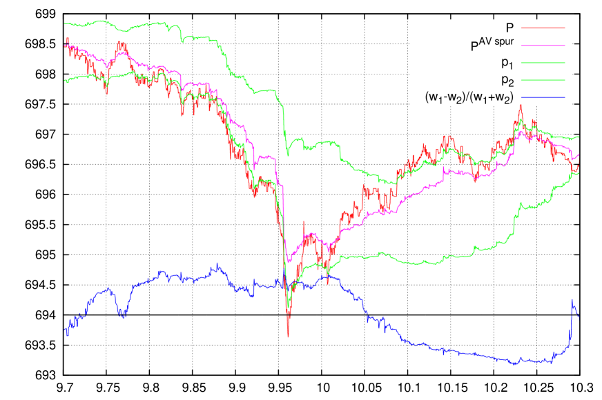
The (106) is $P^{f}$ that, for $\|pI^{f}\|$ operator (54), give the same skewness as the one for $\|I^{f}\|$. This answer is similar to naïve dynamic impact approximation of Section VII.4 (compare (105) with (59), and (106) with (60)). The results are presented in Fig. 12. As for naïve dynamic impact approximation, the $P^{f}$ from (106) behave similar to $P^{[IH]}$ from (61), and have numerical instability for low $\Upsilon$. Future skewness $\widetilde{\Gamma^{0}}_{\mathrm{future}}$ (for $\|I^{f}\|$) is negative (the impact from the future $dI$ (45) make it such). Past skewness $\widetilde{\Gamma^{0}}_{\mathrm{past}}$ (for $\|I\|$) is positive during liquidity deficit and negative during liquidity excess. Trader should open a position during positive $\widetilde{\Gamma^{0}}_{\mathrm{past}}$ and close it during negative $\widetilde{\Gamma^{0}}_{\mathrm{past}}$, this is the only way to avoid catastrophic P&L hit from an unexpected market move.

XI On A Muse of Cash Flow And Liquidity Deficit Existence

We finally reached the point to decide what information can be obtained from historical (time, execution price, shares traded) market observations deploying introduced inMalyshkin and Bakhramov (2015) the dynamic equation: ‘‘Future price tends to the value that maximizes the number of shares traded per unit time’’. While volatility trading is much easier to implement algorithmicallyMalyshkin and Bakhramov (2015), it is much more difficult to implement practically, on exchange, because it requires building some synthetic assets (such as Straddle Wikipedia (2016c)) using options (or other derivatives). Compared to regular HFT equity trading accounts, HFT derivative trading accounts are much more costly and derivative markets often have insufficient available liquidity for a practical trading strategy implementation. In addition to that trading strategies including derivatives are way more difficult to backtest for the reasons of data availability and insufficient liquidity. In this section we are going to discuss whether a much more ambitions goal, to obtain directional price information (not only volatility!), can be practically achieved with the dynamic equation. Our study show, that there are two pieces of information, required to obtain directional information:

First. Price directional information of the past. A trivial information of this type is ‘‘last price minus moving average’’ currently is in common use. We obtained few more sources of this information, having the benefit of automatic time–scale selection. These are: $P^{[IH]}$ (price corresponding to max $I$ on past sample (61)), skewness of price on max $I$ state of $\|p^{m}I^{f}\|$ operator with an impact from the future (Section IX.2), the skewness of price (or P&L) of Section X, and few other.

Second. Execution flow ($I=dV/dt$) directional information. Since Adam SmithWikipedia (2017a) and Karl Marx the volume of the trade is considered to be the key element of goods/money exchange process between buyers and sellers. The concept of Velocity of moneyWikipedia (2017b), velocity of circulation, ($I=dV/dt$ is the velocity of shares, $pI$ is the velocity of money) while being widely recognized as an important macroeconomic concept, is not in use among both academics and exchange trading practitioners (at best they use the volume, assuming the consumption of shares is limited by the number of shares bought: ‘‘The tailor does not attempt to make his own shoes, but buys them of the shoemaker, page 350’’Smith (1827)). Modern exchange trading currently exists of market participants, that are simultaneously buyers and sellers (modern ‘‘shoemaker’’ not only sells the shoes he made, but also buys shoes to sell them later), and, because of leveraged trading, weakly sensitive to the volume $V$ (regular impactWikipedia (2016a)) of the position. As we have shown experimentally, they are much more sensitive to the rate of trading $I=dV/dt$ (dynamic impactMalyshkin (2016)). The situation of market separation of $V$– and $I$– trading can be currently observed in Electricity MarketWikipedia (2017c) that is separated on Energy and Power markets on legislative level. Our exchange experiments show that modern exchange trading is actually a Power–like market. The reason why the velocity of money was not actively used for exchange trading is, from our opinion, the absences of mathematical technique to estimate $I$ (execution flows are non–Gaussian). Because Radon–Nikodym derivatives can be effectively applied to non–Gaussian processes it is the proper tool for velocity of money analysis. Two indicators of $I$ are used in this paper. These are the projections (42) and (43) difference that show whether current $I$ is ‘‘low’’ or ‘‘high’’, and the skewness of $I$, the $\widetilde{\Gamma_{I}}$ from (100) (or more useful in practice $\widetilde{\Gamma^{0}}$ from (103)). The skewness of $I$ can be estimated only from Radon–Nikodym approach, because regular skewness estimators are not applicable for the reason of infinite $\Braket{I^{2}}$ and $\Braket{I^{3}}$.

Practical trading to be this: Determine price direction (e.g. from $P^{[IH]}$ (61)), or the skewness of $P$, Section X.2, with some measure). Then calculate $I$–skewness $\widetilde{\Gamma^{0}}$. Open a position (according to price direction found) when $\widetilde{\Gamma^{0}}$ is close to $1$, close already opened position (but do not take opposite position!) when $\widetilde{\Gamma^{0}}$ is close to $-1$ to avoid catastrophic P&L drain in case of unexpected market move against position held. Such a strategy do provide provide a P&L, and, important, is resilient to unexpected market hits. In the next paper I will try to present a demonstration of this strategy computer implementated. Do not expect a big miracle, (even a ‘‘small miracle’’ of paper trading P&L), but avoiding big P&L hits can also be considered as a miracle of some kind.

Appendix A Time–Distance Between $\psi$ States

For two $\psi$ states from (34), already separated in $I$–space by the value of eigenvalue $\lambda_{I}$, the separation in time space is often required. For this a ‘‘time–distance function’’, $d_{jk}$ between the $\psi^{[j]}_{I}(x)$ and $\psi^{[k]}_{I}(x)$ states from (34) is required. The $d_{jk}$ is an antisymmetric matrix, showing which state $\psi^{[j]}_{I}(x)$ or $\psi^{[k]}_{I}(x)$ is later (in time) and which one is earlier.

$$d_{jk} = -d_{kj}$$ (107)

There are several $d_{jk}$ choices, that can be applied to the task. All of them can be obtained from two–point propagator–like expressions with some antisymmetric $DI(x,y)$

$$DI(x,y) = -DI(y,x)$$ (108)

$$d_{jk} = \int\int DI(x,y)\left(\psi^{[j]}(x)\right)^{2}\left(\psi^{[k]}(y)\right)^{2}d\mu(x)d\mu(y)$$ (109)

These are the most common $DI(x,y)$ choices:

• Probability difference between ‘‘$j$ coming after $k$’’ and ‘‘$j$ coming before $k$’’ events. Can be obtained from (109) with $DI(x,y)=\mathrm{sign}(x-y)$. It can be calculated analytically for the measures (4) and (11). See java classes {KkQVMLegendreShifted, KkQVMLaguerre, KkQVMMonomials}.{_getK2,_getEDPsi} from Appendix G for implementation of probability difference function and infinitesimal time shift operator.

• Total volume traded

  $$V^{[j]} = \frac{\Braket{\psi^{[j]}_{I}}{V}{\psi^{[j]}_{I}}}{\Braket{\psi^{[j]}_{I}}{\psi^{[j]}_{I}}}$$ (110)

  $$d_{jk} = V^{[j]}-V^{[k]}$$ (111)

  Corresponds to (109) with $DI(x,y)=V(x)-V(y)$. The state with a greater volume can be considered as coming after the state with lower volume.

• Difference in projection to $\psi_{0}(x)$ from (39):

  $$d_{jk} = \left(\psi^{[j]}_{I}(x_{0})\right)^{2}-\left(\psi^{[k]}_{I}(x_{0})\right)^{2}$$ (112)

  Corresponds to (109) with $DI(x,y)=D_{x}-D_{y}$, with $D_{x}$ and $D_{y}$– infinitesimal time shift operators on $x$ and $y$. The state with a greater projection to $\psi_{0}(x)$ is considered to be the one coming after the state with lower projection. The distance (112) is degenerated: it is equal to 0 for any two $\psi(x)$ for which $0=\psi(x_{0})$. Also note, that $\psi^{[j]}_{I}(x_{0})=\Braket{\psi^{[j]}_{I}}{\psi_{0}}\psi_{0}(x_{0})$, i.e. the $\psi^{[j]}_{I}(x_{0})$ differ from the $\Braket{\psi^{[j]}_{I}}{\psi_{0}}$ on a constant.

• One can variate the (110) with infinitesimal time shift of $\psi^{[j]}_{I}$, applying (6) or (13) operator to receive (after normalization) a time–distance like this:

  $$\delta V^{[j]} = \Braket{\psi^{[j]}_{I}}{V_{x_{0}}-V}{\psi^{[j]}_{I}}\left(\psi^{[j]}_{I}(x_{0})\right)^{2}-\lambda^{[j]}_{I}$$ (113)

  $$d^{[j]} = \left(\psi^{[j]}_{I}(x_{0})\right)^{2}\frac{\Braket{\psi^{[j]}_{I}}{V_{x_{0}}-V}{\psi^{[j]}_{I}}}{\lambda^{[j]}_{I}}-1$$ (114)

  $$d_{jk} = d^{[j]}-d^{[k]}$$ (115)

  The (114) is a ‘‘second order distance’’. In contrast with the volume (110), the (114) describe the difference in flows of volume since $\psi^{[j]}_{I}$ till ‘‘now’’ per time $\left(\psi^{[j]}_{I}(x_{0})\right)^{2}$ and the rate $\lambda^{[j]}_{I}$.

Appendix B $L^{4}\widetilde{\rho}(p,r)$: Value Correlation of Variables.

For two variables $p$ and $r$, with some positive measure $\Braket{p^{m}r^{q}}=\int p^{m}(t)r^{q}(t)d\mu$ on them, regular $L^{2}covariation$ and a new one $L^{4}covariation$ can be obtained by differentiation (118) and (122):

$$\Braket{(p-\overline{p})^{2}} \to \min$$ (116)

$$\Braket{(r-\overline{r})^{2}} \to \min$$ (117)

$$L^{2}covariation = \frac{1}{4}\frac{\partial}{\partial\overline{p}}\frac{\partial}{\partial\overline{r}}\Braket{(p-\overline{p})^{2}(r-\overline{r})^{2}}$$ (118)

$$L^{2}\rho(p,r) = \frac{\Braket{(p-\overline{p})(r-\overline{r})}}{\sqrt{\Braket{(p-\overline{p})^{2}}\Braket{(r-\overline{r})^{2}}}}$$ (119)

$$\Braket{(p-p_{1})^{2}(p-p_{2})^{2}} \to \min$$ (120)

$$\Braket{(r-r_{1})^{2}(r-r_{2})^{2}} \to \min$$ (121)

$$L^{4}covariation = \frac{1}{16}\frac{\partial}{\partial p_{1}}\frac{\partial}{\partial p_{2}}\frac{\partial}{\partial r_{1}}\frac{\partial}{\partial r_{2}}\Braket{(p-p_{1})^{2}(p-p_{2})^{2}(r-r_{1})^{2}(r-r_{2})^{2}}$$ (122)

$$L^{4}\rho(p,r) = \frac{\Braket{(p-p_{1})(p-p_{2})(r-r_{1})(r-r_{2})}}{\sqrt{\Braket{(p-p_{1})^{2}(p-p_{2})^{2}}\Braket{(r-r_{1})^{2}(r-r_{2})^{2}}}}$$ (123)

where $p_{\{1,2\}}$ and $r_{\{1,2\}}$ are quadrature nodes obtained from (120) and (121) minimization, exactly as we did in Eq. (75) above. The $L^{4}covariation$ (122) (and (123) correlation) covariate $p$ and $r$, but use higher order moments; for $p=r$ it gives regular relations: $L^{4}volatility=L^{4}covariation$, $L^{4}\rho(r,r)=1$ and $L^{4}\rho(r,const)=0$.

A much more interesting case is to consider the matrix $L^{4}covariation_{p_{j},r_{k}}$, that covariate $j$–th level of $p$ with $k$–th level of $r$; (here $j,k=1,2$ and $s=\{p,r\}$). Consider Lagrange interpolating polynomials $l^{(s)}_{k}$ built on quadrature nodes, (they are proportional to (71) eigenfunctions):

$$l^{(s)}_{\{1,2\}}(s) = \frac{s-s_{\{2,1\}}}{s_{\{1,2\}}-s_{\{2,1\}}}$$ (124)

$$l^{(s)}_{\{1,2\}}(s_{\{1,2\}}) = 1$$ (125)

$$l^{(s)}_{\{1,2\}}(s_{\{2,1\}}) = 0$$ (126)

$$w^{(s)}_{\{1,2\}} = \Braket{l^{(s)}_{\{1,2\}}}=\Braket{\left(l^{(s)}_{\{1,2\}}\right)^{2}}$$ (127)

$$\Braket{1} = w^{(s)}_{1}+w^{(s)}_{2}=\int d\mu$$ (128)

$$L^{4}covariation_{p_{j},r_{k}} = \Braket{l^{(p)}_{j}l^{(r)}_{k}}=\int l^{(p)}_{j}(p(t))l^{(r)}_{k}(r(t))d\mu$$ (129)

The $2\times 2$ covariation matrix (129) can be interpreted as a joint distribution matrix of $p$ and $r$ variables. Corresponding to quadrature nodes Lagrange interpolating polynomials $l^{(s)}_{k}$ are a useful tool to built such a matrix, because their inner product can be obtained for the measures of interest. The (129) covariance definitions have integrals over time, that can be calculated directly from distribution moments, it can be obtained from observation sample in a way similar to (7) or (14). For $p=r$ the matrix is diagonal: $L^{4}covariation_{s_{j},s_{k}}=\tiny\left(\begin{array}[]{ll}w^{(s)}_{1}&0\\ 0&w^{(s)}_{2}\end{array}\right)$.

$L^{4}covariation_{p_{j},r_{k}}$ matrix components have the dimension of the measure $\Braket{1}$ from (128) and can be easily written for two–point Gauss quadratures built on $p$ and $r$:

$$L^{4}covariation_{p_{j},r_{k}}=\frac{1}{(p_{1}-p_{2})(r_{1}-r_{2})}\left(\begin{array}[]{ll}\Braket{(p-p_{2})(r-r_{2})}&-\Braket{(p-p_{2})(r-r_{1})}\\ -\Braket{(p-p_{1})(r-r_{2})}&\Braket{(p-p_{1})(r-r_{1})}\end{array}\right)$$ (130)

quadrature weights $w^{(s)}_{\{1,2\}}$can be expressed through $L^{4}covariation_{p_{j},r_{k}}$ elements sum:

$$w^{(p)}_{\{1,2\}} = L^{4}covariation_{p_{\{1,2\}},r_{1}}+L^{4}covariation_{p_{\{1,2\}},r_{2}}$$ (131a)

$$w^{(r)}_{\{1,2\}} = L^{4}covariation_{p_{1},r_{\{1,2\}}}+L^{4}covariation_{p_{2},r_{\{1,2\}}}$$ (131b)

From (130) immediately follow that the sum of all four elements of $L^{4}covariation_{p_{j},r_{k}}$ matrix is equal to $\Braket{1}$ . To obtain dimensionless ‘‘correlation’’–like matrix the (130) can be divided by $\Braket{1}$ from (128), the difference between diagonal and off-diagonal elements of this ‘‘correlation’’–like matrix can be called $L^{4}\widetilde{\rho}(p,r)$ correlation:

$$L^{4}\widetilde{\rho}(p,r) = \frac{\sum\limits_{j,k=1}^{2}(-1)^{j-k}\,L^{4}covariation_{p_{j},r_{k}}}{\sum\limits_{j,k=1}^{2}L^{4}covariation_{p_{j},r_{k}}}$$ (132)

$$L^{4}\widetilde{\rho}(p,r) = \frac{\overline{pr}-\overline{p}\,\overline{r}+\left(\frac{p_{1}+p_{2}}{2}-\overline{p}\right)\left(\frac{r_{1}+r_{2}}{2}-\overline{r}\right)}{0.25(p_{1}-p_{2})(r_{1}-r_{2})}$$ (133)

that is different from regular definition by the term $\left(\frac{p_{1}+p_{2}}{2}-\overline{p}\right)\left(\frac{r_{1}+r_{2}}{2}-\overline{r}\right)$ describing skewness correlation. The (133) means, that if two distributions have the skewness of the same sign, their ‘‘true’’ correlation is actually higher, than the one, calculated from the lower order moments as $\overline{pr}-\overline{p}\,\overline{r}$. The (133) formula for $L^{4}\widetilde{\rho}(p,r)$ is obtained directly from joint distribution matrix (130) and has a meaning of values correlation: the $L^{4}covariation_{p_{j},r_{k}}$ element of (129) matrix is the probability that $p=p_{j}$ and $r=r_{k}$. The conditions $L^{4}\widetilde{\rho}(r,r)=1$ and $L^{4}\widetilde{\rho}(r,const)=0$ also holds, same as for $L^{4}\rho(p,r)$ from (123). We want to emphasize, that, in applications, the most intriguing feature is not a new formula (133) or (123) for correlation, but an ability to obtain $(p,r)$ joint distribution matrix (130) from sampled moments of two distributions.

Quadrature nodes $p_{\{1,2\}}$ and $r_{\{1,2\}}$ are calculated from the moments (134a) and (134b) respectively applying either formula (72) above or the ones from Appendix C of Ref. Malyshkin and Bakhramov (2015) (or the formulas from Appendix D of this paper with $dI=0$, what give $P^{f}$–independent answers). For $\Braket{pr}$ term in (130) one more moment (cross–moment) $(\pi\rho)_{1}$ from (134c) is required in addition to regular $\pi_{m}$ and $\rho_{m}$ ($m=0,1,2,3$):

$$\pi_{m} = \Braket{p^{m}}$$ (134a)

$$\rho_{m} = \Braket{r^{m}}$$ (134b)

$$(\pi\rho)_{1} = \Braket{pr}$$ (134c)

(to calculate (130) matrix it requires total 8 moment, see the file com/polytechnik/utils/ValueCorrelation.java for implementation example of numerical calculation of value correlation). The (134) definitions can be be generalized to matrix averages (see Appendix E of Ref.Malyshkin and Bakhramov (2015)), that corresponds to mixed state in quantum mechanics, a generalization from pure states of $\Braket{\psi}{p^{m}r^{q}I}{\psi}$ form.

Appendix C $\widetilde{\rho}(f,g)$: Probability Correlation of Variables.

Obtained from sampled moments joint distribution estimator (130) of previous appendix is an important step in correlation estimation. However, it still has a number of limitations to be applied to practical data.

1. It requires two quadratures (on $p$ and $r$) to be built, this requires the moments (134) to be calculated from the data. Assume $r$ is execution flow $r=I=dv/dt$ of some security, then, for example, $\Braket{r^{2}}$ is problematic to calculate: it is not possible to calculate it directly from sample and (50) approach does not always give a good result.

2. The cross–moment $(\pi\rho)_{1}$ from (134c) is often problematic to calculate.

3. Some of (134) moments can diverge or even do not exist, their numerical estimation often becomes a kind of numerical regularization exercise.

If we generalize ‘‘correlation concept’’, then the approach to joint distribution matrix estimation can be extended to using the moments calculated in arbitrary basis, not only for the one with basis functions argument as an observable, the case considered in Appendix B. Assume we have two variables $f$ and $g$ (e.g. execution flow of two securities), some basis $Q_{m}(x)$ for $m=0,1,2$ ($x$ can be e.g. time or price; $Q_{m}(x)$ is a polynomial of $m$–th order), inner product $\Braket{Q_{j}(x)}{s}{Q_{k}(x)}$ (where $s=\{f,g,const\}$ and $j,k=0,1$) is defined in some way, such that the inner product can be calculated directly from sample. As we discussed in Bobyl et al. (2016) any observable variable sample can be converted to a matrix, then generalized eigenvalue problems define the spectrum of the observable. For $f$ and $g$ this would be the equations (similar to Eq. (33) with $n=2$):

$$\sum\limits_{k=0}^{1}\Braket{Q_{j}}{f}{Q_{k}}\alpha^{f;[i]}_{k} = \lambda^{[i]}_{f}\sum\limits_{k=0}^{1}\Braket{Q_{j}}{Q_{k}}\alpha^{f;[i]}_{k}$$ (135)

$$\sum\limits_{k=0}^{1}\Braket{Q_{j}}{g}{Q_{k}}\alpha^{g;[i]}_{k} = \lambda^{[i]}_{g}\sum\limits_{k=0}^{1}\Braket{Q_{j}}{Q_{k}}\alpha^{g;[i]}_{k}$$ (136)

For $n=2$ generalized eigenvalue problem $\Ket{A|\psi}=\lambda\Ket{B|\psi}$ is reduced to solving quadratic on $\lambda$ equation: $0=\det\|A-\lambda B\|$, same as with Eq. (71):

$$\left(\begin{array}[]{ll}\Braket{Q_{0}}{s}{Q_{0}}&\Braket{Q_{0}}{s}{Q_{1}}\\ \Braket{Q_{1}}{s}{Q_{0}}&\Braket{Q_{1}}{s}{Q_{1}}\end{array}\right)\left(\begin{array}[]{l}\alpha_{0}^{s;[i]}\\ \alpha_{1}^{s;[i]}\end{array}\right) = \lambda_{s}^{[i]}\left(\begin{array}[]{ll}\Braket{Q_{0}}{Q_{0}}&\Braket{Q_{0}}{Q_{1}}\\ \Braket{Q_{1}}{Q_{0}}&\Braket{Q_{1}}{Q_{1}}\end{array}\right)\left(\begin{array}[]{l}\alpha_{0}^{s;[i]}\\ \alpha_{1}^{s;[i]}\end{array}\right)$$ (145)

$$\Ket{\psi^{[i]}_{s}}\,\,\mathrm{state} : \psi^{[i]}_{s}(x)=\alpha_{0}^{s;[i]}Q_{0}(x)+\alpha_{1}^{s;[i]}Q_{1}(x)$$ (146)

Found $\frac{\Braket{s\psi^{2}(x)}}{\Braket{\psi^{2}(x)}}\to\{\min;\max\}$ solutions are chosen to have normalized $\Ket{\psi^{[i]}_{s}}$ eigenvectors: $\delta_{im}=\sum\limits_{j,k=0}^{1}\alpha^{s;[i]}_{j}\Braket{Q_{j}}{Q_{k}}\alpha^{s;[m]}_{k}$ ; $\lambda_{s}^{[i]}=\Braket{\psi^{[i]}_{s}}{s}{\psi^{[i]}_{s}}$, and ordered eigenvalues $\lambda^{[0]}_{\{f,g\}}\leq\lambda^{[1]}_{\{f,g\}}$. The square of eigenvectors scalar product define $2\times 2$ matrix $Pcorrelation_{\lambda^{[i]}_{f},\lambda^{[m]}_{g}}$, the elements of which are the probabilities of how low/high $f$ is correlated to low/high $g$:

$$Pcorrelation_{\lambda^{[i]}_{f},\lambda^{[m]}_{g}} = \left(\sum\limits_{j,k=0}^{1}\alpha^{f;[i]}_{j}\Braket{Q_{j}}{Q_{k}}\alpha^{g;[m]}_{k}\right)^{2}$$ (147)

$$\widetilde{\rho}(f,g) = \frac{\sum\limits_{i,m=0}^{1}(-1)^{i-m}\,Pcorrelation_{\lambda^{[i]}_{f},\lambda^{[m]}_{g}}}{\sum\limits_{i,m=0}^{1}Pcorrelation_{\lambda^{[i]}_{f},\lambda^{[m]}_{g}}}$$ (148)

The $\widetilde{\rho}(f,g)$ modified correlation is the difference between diagonal and off-diagonal elements of $Pcorrelation_{\lambda^{[i]}_{f},\lambda^{[m]}_{g}}$ matrix. This is similar to (132) of previous section, but now the $Pcorrelation_{\lambda^{[i]}_{f},\lambda^{[m]}_{g}}$ matrix is built solely out from $\Braket{Q_{j}}{s}{Q_{k}}$ moments, that can be defined in arbitrary basis. An important difference between (147) and (129) matrices is that the (129) elements are scalar product of eigenvectors, but (147) elements are squared scalar product of eigenvectors; the elements of both matrices have a meaning of probability, but the probability is defined differently. The (147), as squared scalar product of eigenvectors, is a correlation of probabilities. The $Pcorrelation_{\lambda^{[i]}_{f},\lambda^{[m]}_{g}}$ is a probability of probability that $f$ has a value $\lambda^{[i]}_{f}$ and $g$ has a value $\lambda^{[m]}_{g}$, what is different from the $L^{4}covariation_{p_{j},r_{k}}$, Eq. (129), that is a probability of $p=p_{j}$ and $r=r_{k}$. Instead of (131) we now have:

$$1 = Pcorrelation_{\lambda^{[\{0,1\}]}_{f},\lambda^{[0]}_{g}}+Pcorrelation_{\lambda^{[\{0,1\}]}_{f},\lambda^{[1]}_{g}}$$ (149a)

$$1 = Pcorrelation_{\lambda^{[0]}_{f},\lambda^{[\{0,1\}]}_{g}}+Pcorrelation_{\lambda^{[1]}_{f},\lambda^{[\{0,1\}]}_{g}}$$ (149b)

the sum of the elements in any row or column of $Pcorrelation_{\lambda^{[i]}_{f},\lambda^{[m]}_{g}}$ matrix is equal to $1$. If $Q_{0}(x)=const$ (typical situation), then, similar to (74) definition, a skewness–like (like a difference between median and average) characteristics $\widetilde{\Gamma}$ of random variable $s=\{f,g\}$ can be introduced:

$$\widetilde{\Gamma} = \frac{2\overline{s}-\lambda^{[0]}_{s}-\lambda^{[1]}_{s}}{\lambda^{[0]}_{s}-\lambda^{[1]}_{s}}$$ (150)

$$\overline{s} = \Braket{sQ_{0}}\Big{/}\Braket{Q_{0}}$$ (151)

$$\widetilde{\rho}(f,g) = \frac{\Braket{\psi^{[0]}_{g}}{f}{\psi^{[0]}_{g}}-\Braket{\psi^{[1]}_{g}}{f}{\psi^{[1]}_{g}}}{\lambda^{[0]}_{f}-\lambda^{[1]}_{f}}$$ (152)

$$= \frac{\Braket{\psi^{[0]}_{g}}{f}{\psi^{[0]}_{g}}-\Braket{\psi^{[1]}_{g}}{f}{\psi^{[1]}_{g}}}{\Braket{\psi^{[0]}_{f}}{f}{\psi^{[0]}_{f}}-\Braket{\psi^{[1]}_{f}}{f}{\psi^{[1]}_{f}}}$$ (153)

This skewness definition (150) has a meaning of $\psi(x)=const$ state $\Ket{\psi_{C}}$ expansion weights asymmetry on the states: $\Ket{\psi^{[0]}_{s}}$, corresponding to minimal $s=\lambda^{[0]}_{s}$, and $\Ket{\psi^{[1]}_{s}}$, corresponding to maximal $s=\lambda^{[1]}_{s}$; $\widetilde{\Gamma}=\Braket{\psi_{C}}{\psi^{[0]}_{s}}^{2}-\Braket{\psi_{C}}{\psi^{[1]}_{s}}^{2}$. The (148) probability correlation $\widetilde{\rho}(f,g)$ can be also written in a similar ‘‘derivative–like’’ form (152): the difference between $f$ in the state $\Ket{\psi^{[0]}_{g}}$ of minimal $g$, and $f$ in the state $\Ket{\psi^{[1]}_{g}}$ of maximal $g$, divided by minimal and maximal $f$ difference. For probability correlation classical condition $\widetilde{\rho}(f,f)=1$ holds, for $f=g$ the (147) matrix is diagonal: $Pcorrelation_{\lambda^{[i]}_{f},\lambda^{[m]}_{f}}=\tiny\left(\begin{array}[]{ll}1&0\\ 0&1\end{array}\right)$. But another classical condition does not hold: $\widetilde{\rho}(f,const)\neq 0$, if $g=const$ then eigenvalues problem (136) is degenerated and, without an extra condition on eigenvectors, the value of probability correlation (148) can be arbitrary, depending on specific $g$– eigenvectors choice.

The distinction between ‘‘value’’ and ‘‘probability’’ correlations is an important topic of modern research in both computer science and market dynamics. The problems of Distribution Regression ProblemDietterich et al. (1997); Zhou (2004) (a number of observations of type ‘‘bag of instances to a value’’ are used to build a mapping: probability distribution to value) and Distribution to Distribution Regression Problem (a number of observations of type ‘‘bag of instances to a bag of other instances’’ are used to build a mapping: probability distribution to probability distribution) are the most known generalization of regular Regression Problem (a number of observations of type ‘‘value to a value’’ are used to build a mapping: value to value) have been addressed from a number of points. Our contribution to it is based on an application of Christoffel functionMalyshkin (2015c), and Radon–Nikodym derivativesMalyshkin (2015d). The difficulties in probability estimation using real life data have been emphasizedTaleb et al. (2014), but very different mathematical technique have been used for probability estimation. The (148) answer is, to the best of our knowledge, the first probability correlation answer, that is calculated from the moments of sampled data. To calculate (147) matrix it requires $m=0,1,2$ moments: $\Braket{\{f,g,const\}Q_{m}(x)}$; total 9 moment, see the file com/polytechnik/utils/ProbabilityCorrelation.java for implementation example of numerical calculation of probability correlation $\widetilde{\rho}(f,g)$ from (148), also see the file com/polytechnik/utils/Skewness.java:getGSkewness for calculation $\widetilde{\Gamma}$ from (150). A remarkable feature of these answers is that they use only first order moments on $f$ and $g$ and higher order moments on $Q_{m}(x)$. This separation of observable variables and basis functions allows the approach to be applied to $f$ and $g$ having non–Gaussian distributions, even those with, say, infinite $\Braket{f^{2}}$ or $\Braket{g^{2}}$, a distinguishable feature of Radon–Nikodym approachBobyl et al. (2016).

Appendix D Price distribution estimation with unknown future price $P^{f}$ as a parameter

Figure 13: Several examples of $\Gamma(P^{f})$ dependence for different $\pi_{m}$ and $di$. The $\Gamma(P^{f})$ has maximum and minimum at unperturbed ($di=0$) quadrature nodes; the $P^{f}\to\pm\infty$ asymptotic is (162). Dashed line is $\Gamma(P^{f})$ skewness for the measure with single support at average value (single node quadrature).

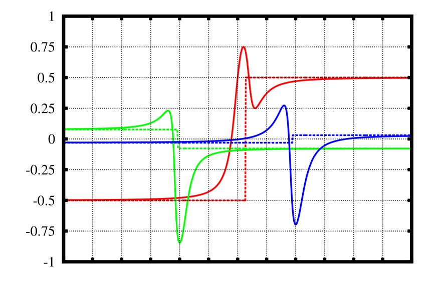
In Section VIII we solved the problem of price distribution estimation given $\pi_{m}$ moments (62). However, future price $P^{f}$ is required to calculate future moments $\pi_{m}^{f}$; ‘‘the last price as $P^{f}$ estimator (55)’’ is a very crude approximation, thus it is better to consider $P^{f}$ as a parameter (This consideration is a special case of varying measures orthogonal polynomialsTotik (11 Nov. 2005). In this work, instead of typicaly considered a sequence of measures, a measure, depending on $P^{f}$ as a parameter, is considered.) For a given $\Ket{\psi}$ the $\|p^{m}I^{f}\|$ operator from (54) with an impact from the future term give future moments $\pi_{m}^{f}$:

$$\pi_{m}^{f} = \pi_{m}+\left(P^{f}\right)^{m}dI\Braket{\psi}{\psi_{0}}^{2}$$ (154)

that are different from past moments $\pi_{m}=\Braket{\psi}{p^{m}I}{\psi}$ from (62) by impact from the future term: $\left(P^{f}\right)^{m}dI\Braket{\psi}{\psi_{0}}^{2}$. The value of $P^{f}$ is unknown, however one can repeat all the calculations of Section VIII above, using $P^{f}$ as a parameter. After simple algebra (see DiffSkewness.java from Appendix G below for numerical implementation) $P^{f}$–dependent $\Gamma$ from (74), quadrature nodes $p_{\{1,2\}}(P^{f})$, weights $w_{\{1,2\}}(P^{f})$, and monic second order orthogonal polynomial (168) ($P^{f}$ –dependent orthogonal system) for the measure with (154) moments are:

$$di = dI\Braket{\psi}{\psi_{0}}^{2}$$ (155)

$$b = \frac{di}{\pi_{0}+di}$$ (156)

$$a_{m} = \frac{\pi_{m}}{\pi_{0}+di}$$ (157)

$$A(P^{f}) = (a_{3}a_{1}-a_{2}^{2})+(a_{3}b)P^{f}-2(a_{2}b)\left(P^{f}\right)^{2}+(a_{1}b)\left(P^{f}\right)^{3}$$ (158)

$$B(P^{f}) = (a_{2}a_{1}-a_{3})+(a_{2}b)P^{f}+(a_{1}b)\left(P^{f}\right)^{2}-(1-b)b\left(P^{f}\right)^{3}$$ (159)

$$D(P^{f}) = (a_{2}-a_{1}^{2})-2(a_{1}b)P^{f}+(1-b)b\left(P^{f}\right)^{2}$$ (160)

$$\Gamma(P^{f}) = \frac{-B(P^{f})-2(a_{1}+bP^{f})D(P^{f})}{\sqrt{B^{2}(P^{f})-4A(P^{f})D(P^{f})}}$$ (161)

$$\Gamma(P^{f}\to\pm\infty) = \pm\frac{\pi_{0}-di}{\pi_{0}+di}$$ (162)

$$p_{\{1,2\}}(P^{f}) = \frac{-B(P^{f})\mp\sqrt{B^{2}(P^{f})-4A(P^{f})D(P^{f})}}{2D(P^{f})}$$ (163)

$$w_{\{1,2\}}(P^{f}) = \frac{\pi_{0}+di}{1+\left.{\left[p_{\{1,2\}}(P^{f})-\overline{p}(P^{f})\right]^{2}}\right/{D(P^{f})}}$$ (164)

$$\overline{p}(P^{f}) = \frac{p_{1}(P^{f})w_{1}(P^{f})+p_{2}(P^{f})w_{2}(P^{f})}{w_{1}(P^{f})+w_{2}(P^{f})}=a_{1}+bP^{f}$$ (165)

$$p_{mid}(P^{f}) = \frac{p_{1}(P^{f})+p_{2}(P^{f})}{2}=-0.5\frac{B(P^{f})}{D(P^{f})}$$ (166)

$$p_{2}(P^{f})-p_{1}(P^{f}) = \frac{\sqrt{B^{2}(P^{f})-4A(P^{f})D(P^{f})}}{D(P^{f})}$$ (167)

$$P_{2}(p,P^{f}) = (p-p_{1}(P^{f}))(p-p_{2}(P^{f}))=p^{2}+\frac{B(P^{f})}{D(P^{f})}p+\frac{A(P^{f})}{D(P^{f})}$$ (168)

$$E(P^{f}) = (a_{3}a_{1}-a_{2}^{2})+(a_{2}a_{1}-a_{3}(1-b))P^{f}+(a_{2}(1-b)-a_{1}^{2})\left(P^{f}\right)^{2}$$

$$\overline{(p-p_{1}(P^{f}))^{2}(p-p_{2}(P^{f}))^{2}} = a_{4}+\frac{a_{3}B(P^{f})+a_{2}A(P^{f})+(P^{f})^{2}bE(P^{f})}{D(P^{f})}$$ (169)

$$\overline{(p-\overline{p}(P^{f}))^{2}} = D(P^{f})$$ (170)

The (161) is a ratio of third order polynomial in numerator and square root of sixth order polynomial in denominator. The $\Gamma(P^{f})$ is a function with $\frac{w_{1}-w_{2}+di}{w_{1}+w_{2}+di}$ maximum at $P^{f}=p_{1}$ and $\frac{w_{1}-w_{2}-di}{w_{1}+w_{2}+di}$ minimum at $P^{f}=p_{2}$, $p_{1}\leq p_{2}$, where $p_{\{1,2\}}$ and $w_{\{1,2\}}$ are quadrature nodes and weights of two–point Gauss quadrature built on $\pi_{m}$ moments (with $di=0$, unperturbed quadrature: $w_{1}+w_{2}=\pi_{0}$). The $\Gamma(P^{f})$ have (162) asymptotic for $P^{f}\to\pm\infty$. In Fig. 13 several examples for $\Gamma(P^{f})$ are presented, maximum, minimum and asymptotic are clearly observed.

When $\pi_{m}$ moments are of single support point distribution the (161) take a very simple form: Gauss quadrature built on $\pi^{f}_{m}$ moments (154) has the nodes: the support point and $P^{f}$; quadrature weights are: $\pi_{0}$ and $di$; the $\Gamma(P^{f})$ is a step–function with (162) values, changing the value at support point; $L^{4}volatility$ from (75) is zero. In Fig. 13 this situation: two support points: unperturbed average (with the weight $w_{1}+w_{2}$) and $P^{f}$ (with the weight $di$) is presented as dashed lines.

Figure 14: An example of distribution (with $p_{1}=0.1$, $w_{1}=1$, $p_{2}=0.3$, $w_{2}=0.2$). Top: The dependence (163) of $p_{1}(P^{f})$ (red) and $p_{2}(P^{f})$ (green) for $di=0.4$ (solid lines) and $di\to\infty$ asymptotic (dashed lines). Bottom: The dependence (164) of $w_{1}(P^{f})$ (red) and $w_{2}(P^{f})$ (green) for $di=0.4$

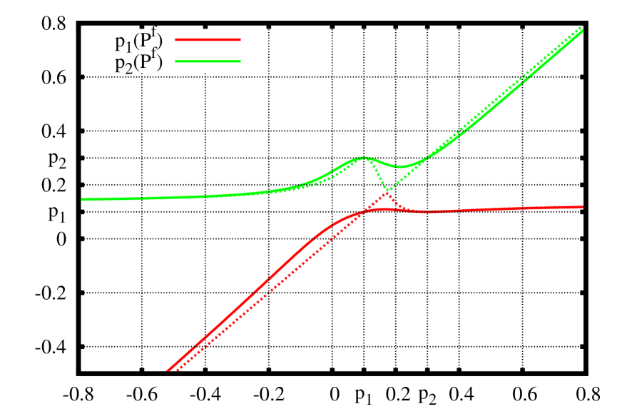
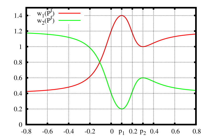
The $p_{\{1,2\}}(P^{f})$ and $w_{\{1,2\}}(P^{f})$ (perturbed quadrature nodes and weights) from (163) and (164) are often of interest. In Fig. 14 we present an example. The weight $w_{\{1,2\}}(P^{f})$ has $w_{\{1,2\}}+di$ maximum at $P^{f}=p_{\{1,2\}}$ and $w_{\{1,2\}}$ minimum at $P^{f}=p_{\{2,1\}}$. The $p_{1}(P^{f})$ is a function with minimum (equal to unperturbed $p_{1}$) at $P^{f}=p_{2}$ and $p_{2}(P^{f})$ is a function with maximimin (equal to unperturbed $p_{2}$) at $P^{f}=p_{1}$, (parabolic behavior of $p_{\{1,2\}}(p_{\{2,1\}}+\Delta p)$ for small $\Delta p$; also note that $p_{\{1,2\}}(p_{\{1,2\}})=p_{\{1,2\}}(p_{\{2,1\}})=p_{\{1,2\}}$). The behavior of $p_{\{1,2\}}(P^{f})$ for a constant $di$ and $di\to\infty$ asymptotic is shown in Fig. 14 as solid and dashed lines respectively. In applications the (166) midpoint (a function with min, max, having $p_{mid}(p_{1})=p_{mid}(p_{2})=p_{mid}(\overline{p})$); the (165) average (a linear function with $b$ slope) can be also of interest.

A very important characteristic is ‘‘volatility’’–like characteristic (167), the difference between perturbed quadrature nodes: $p_{2}(P^{f})-p_{1}(P^{f})$. It is always positive, has the dimension of price and can be used in place of standard deviation. This difference reach the same value $p_{2}-p_{1}$ for $P^{f}$ equal to unperturbed quadrature nodes $p_{\{1,2\}}$ and has $|P^{f}-\overline{p}|$ asymptotic for $P^{f}\to\pm\infty$.

Appendix E P&L Trading Strategy and Frontrun Asymmetry

Figure 15: Top Left: past information available for $\Ket{\psi}$ state: $w_{1}$ at $p_{1}$ and $w_{2}$ at $p_{2}$, where $p_{\{1,2\}}$ and $w_{\{1,2\}}$ are unperturbed quadrature nodes and weights built on past moments (62); the median is $w_{1}$, because $w_{1}>w_{2}$. Top Right: past and future information for $\Ket{\psi}$ state, in addition to the data from ‘‘the past’’ the following is also available: known (155) impact from the future $di$ at unknown future price $P^{f}$. Bottom: ‘‘Band structure’’ of Long/Short frontrunning alternatives. The asymmetry is determined by ‘‘effective mass’’ difference (179).

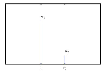
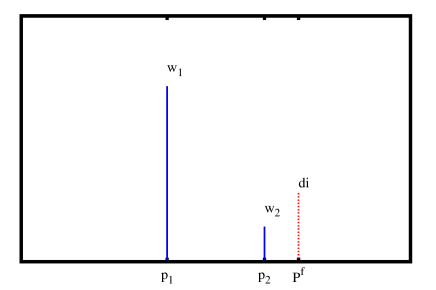
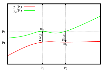
In Section X.2 we considered a simple frontrun strategy and have shown that the median should be used as a threshold. It is of great interest to consider such a strategy in general case. Important feature of trading distributions is that it is a discrete one (price levels are discrete). Moreover, ‘‘real’’ distribution can be interpolated by Gauss quadrature and discrete weights of the quadrature can be considered as interpolating distribution.

Consider a very simple example: let trading take place at price $p_{1}$ with volume $w_{1}$ and at price $p_{2}$ with volume $w_{2}$, Fig. 15 (we assume $p_{1}<p_{2}$, and the $w_{\{1,2\}}$ is the number of matched buyers & sellers at price $p_{\{1,2\}}$). This distribution has the median equal to $p_{1}$ or $p_{2}$, depending what weight $w_{1}$ or $w_{2}$ is a greater one. As in Section X.2, were a speculator knows future trading profile, buying below median and selling above the median, the maximal P&L a speculator can obtain is:

$$\mathrm{P\&L_{\max}} = (p_{2}-p_{1})\min(w_{1},w_{2})$$ (171)

At $p_{1}$ he should frontrun the buyers bidding at $p_{1}+\delta$ and at $p_{2}$ he should frontrun the sellers offering at $p_{2}-\delta$, maximal volume $\min(w_{1},w_{2})$ come from the fact that at the level of highest weight (equal to the median) the speculator have to partially trade both long and short to avoid position accumulation at the end of investment horizon. (If $p_{1}$ and $p_{2}$ are considered as unmatched levels of limit order book — this two–level example is a classical demonstration of market–making, but the whole point of this paper is a transition from unmatched volume (supply/demand) to describing matched data execution flow $I=dV/dt$ (both past and future (45)). This allows us to avoid using (unmeasurable from the data) supply and demand and, instead, to work with (directly measurable from the data) execution flow fluctuations). Similary, for $n$–point distribution (either actual or the weights of Gauss quadrature, built out of $0\dots 2n-1$ distribution moments), one need to find quadrature nodes, the median, then frontrun the buyers below median, frontrun the sellers above median; at the median partially trade both long and short to avoid position accumulation. The P&L calculations is very similar to Quantile regression problem Wikipedia (2016d), but we will not discuss this relation here. In this paper we are going to limit ourselves to two–nodes distributions only, then all the calculations can be performed without full blown Linear Programming theory.

In real life we do not know complete future trading profile. We know impact from the future $di$ from (155), but at unknown future price $P^{f}$, see Fig. 15 right. As with any two–level Hamiltonian arbitrary state can be expanded as a superposition of two–level states. If $P^{f}$ was traded at $p_{1}$ (frontrun buyers), then $w_{1}\to w_{1}+di$, $w_{2}\to w_{2}$. If $P^{f}$ was traded at $p_{2}$ (frontrun sellers), then $w_{1}\to w_{1}$, $w_{2}\to w_{2}+di$. (In both cases $p_{\{1,2\}}$ do not change.). These two alternatives (frontrun buyers/frontrun sellers) give identical price change, and, if $di\leq w_{\{1,2\}}$, also give identical maximal P&L. Otherwise a term $\min(di,w_{\{1,2\}})$ similar to the one in (171) arise.

To obtain directional information we need a criteria to distinguish the two alternatives. They can be distinguished considering variations of $P^{f}$. Assume execution flow to occur not at specific single price $P^{f}$, but within some price interval $P^{f}\pm\Delta p$. Note that according to time–price symmetry argumentMalyshkin and Bakhramov (2015) first order derivative cannot privide dynamics information, thus the P&L should be invariant with respect to $\Delta p\to-\Delta p$. Consider the P&L corresponding to impact from the future execution flow $di$, with $P^{f}$, distributed within the $p_{\{1,2\}}\pm\Delta p$ interval. Then

$$\mathrm{P\&L_{fr\,long}}(P^{f}) = (p_{2}(P^{f})-P^{f})\min(di,w_{2})$$ (172)

$$\mathrm{P\&L_{fr\,short}}(P^{f}) = (P^{f}-p_{1}(P^{f}))\min(di,w_{1})$$ (173)

$$\Delta\mathrm{P\&L_{fr}} = \mathrm{P\&L_{fr\,long}}(p_{2}\pm\Delta p)-\mathrm{P\&L_{fr\,short}}(p_{2}\pm\Delta p)$$ (174)

The $p_{\{1,2\}}(P^{f})$ is a function with min/max at $P^{f}=p_{\{2,1\}}$, see Appendix D Fig. 14. Long/short assymetry (174), can be considered as directional asymmetry and for infinitesimal $\Delta p$ second order term is:

$$\Delta\mathrm{P\&L_{fr}} \approx \frac{(\Delta p)^{2}}{2}\left[\left.\frac{\partial^{2}\mathrm{P\&L_{fr\,long}}(P^{f})}{\partial(P^{f})^{2}}\right|_{P^{f}=p_{1}}-\left.\frac{\partial^{2}\mathrm{P\&L_{fr\,short}}(P^{f})}{\partial(P^{f})^{2}}\right|_{P^{f}=p_{2}}\right]$$ (175)

$$= \frac{(\Delta p)^{2}}{2}\left[\left.\min(di,w_{2})\frac{\partial^{2}p_{2}(P^{f})}{\partial(P^{f})^{2}}\right|_{P^{f}=p_{1}}+\left.\min(di,w_{1})\frac{\partial^{2}p_{1}(P^{f})}{\partial(P^{f})^{2}}\right|_{P^{f}=p_{2}}\right]$$ (176)

The $p_{\{1,2\}}(P^{f})$ are similar to solid state physics ‘‘band structure’’. It is convinient to introduce an ‘‘effective mass’’ near zone edge:

$$\frac{1}{m_{1}} = \left.\frac{\partial^{2}p_{1}(P^{f})}{\partial(P^{f})^{2}}\right|_{P^{f}=p_{2}}$$ (177)

$$\frac{1}{m_{2}} = \left.\frac{\partial^{2}p_{2}(P^{f})}{\partial(P^{f})^{2}}\right|_{P^{f}=p_{1}}$$ (178)

$${\cal D} = \frac{1}{m_{1}}+\frac{1}{m_{2}}$$ (179)

We have $m_{1}>0$ and $m_{2}<0$, as for electrons and holes in a semiconductor, see Fig. 15 for this ‘‘transition’’ analogy. The ${\cal D}$, directional assymetry of distribution, is related to distribution skewness (74) and, in some situations, can be used as a directional indicator.

Appendix F Future Wavefunction Without $I_{0}^{f}$.

In the section VII.3 we have determined (44) future $I_{0}^{f}$ and made an attempt to convert this information to price information using the dynamic equation of Ref. Malyshkin and Bakhramov (2015). A question arise what kind of answer can be obtained without information about $I_{0}^{f}$? It is clear, that in this case only perturbation theory on ${dI}/{I_{0}^{f}}$ can be developed. Because $dI\geq 0$ (46) some information can still be obtained, even in case of unknown $I_{0}^{f}$ value.

Figure 16: The AAPL stock price on September, 20, 2012. Calculated in Shifted Legendre basis with $n=7$ and $\tau$=128sec. The $P^{[IH]}$, $P_{1}$ and $P_{2}$ are calculated according to (61), (191) and (192) respectively.

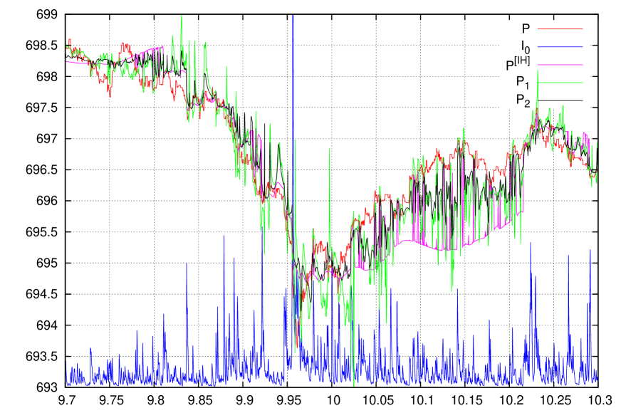
Consider some wavefunction $\psi(x)$ and corresponding execution flow $I_{\psi}$, calculated as in (24). Consider simple variation $\delta\psi(x)$. Then second order Rayleigh quotient perturbation is:

$$I_{\psi+\delta\psi} = \frac{\Braket{\psi+\delta\psi}{I}{\psi+\delta\psi}}{\Braket{\psi+\delta\psi}{\psi+\delta\psi}}=D0+D1+D2+\dots$$ (180)

$$D0 = \frac{\Braket{\psi}{I}{\psi}}{\Braket{\psi}{\psi}}$$ (181)

$$D1 = 2\left(\frac{\Braket{\psi}{I}{\delta\psi}}{\Braket{\psi}{\psi}}-D0\frac{\Braket{\psi}{\delta\psi}}{\Braket{\psi}{\psi}}\right)$$ (182)

$$D2 = \frac{\Braket{\delta\psi}{I}{\delta\psi}}{\Braket{\psi}{\psi}}-D0\frac{\Braket{\delta\psi}{\delta\psi}}{\Braket{\psi}{\psi}}-2\frac{\Braket{\psi}{\delta\psi}}{\Braket{\psi}{\psi}}D1$$ (183)

A rather complex perturbation theory on $\Ket{\delta\psi}$ can be developed in a style of our earlier work Malyshkin et al. (1999) in a very different field of multiple-scattering, but we limit here all the considerations to first order $I$ variation only on $\delta\psi$ states, orthogonal to $\psi$, i.e. $\Braket{\delta\psi}{\psi}=0$. Then

$$I_{\psi+\delta\psi} \approx \frac{\Braket{\psi}{I}{\psi}}{\Braket{\psi}{\psi}}+\delta I$$ (184)

$$\delta I = 2\frac{\Braket{\psi}{I}{\delta\psi}}{\Braket{\psi}{\psi}}=2\Braket{b}{\delta\psi}$$ (185)

$$\Ket{b} = \Ket{I|\psi}$$ (186)

Thus $\delta I$ (185) is represented as a scalar product of $\Ket{b}$ and $\Ket{\delta\psi}$ vectors. What variation $\delta\psi$ to provide maximal $\delta I$? The one, different from $\Ket{b}$ only on a constant $\beta$, i.e.

$$\Ket{\phi} = \Ket{I|\psi}-\Braket{\psi}{I}{\psi}\Ket{\psi}$$ (187)

$$\Ket{\delta\psi} = \Ket{\phi}\beta$$ (188)

The states (188) provide maximal variation $\delta I$. The term $\Braket{\psi}{I}{\psi}\Ket{\psi}$ is subtracted in (187) to have $\Braket{\delta\psi}{\psi}=0$. Put $\Ket{\psi}=\Ket{\psi_{0}}$ from Eq. (39) to (187), this immediately lead to $\phi(x_{0})=0$, and consider $I$ as a function of $\beta$

$$\Ket{\phi} = \Ket{I|\psi_{0}}-\Braket{\psi_{0}}{I}{\psi_{0}}\Ket{\psi_{0}}$$ (189)

$$I(\beta) = \frac{\Braket{\psi_{0}+\beta\phi}{I}{\psi_{0}+\beta\phi}}{\Braket{\psi_{0}+\beta\phi}{\psi_{0}+\beta\phi}}$$ (190)

$$\approx I_{0}+2\beta\Braket{\phi}{I}{\psi_{0}}+\dots$$

As we noted in section VII.1 when $\Ket{\psi_{0}}$ is an eigenfunction of (33) (or $I=const$ and the problem (33) is degenerated), then theory fails (now for the reason of $\Braket{\phi}{\phi}=0$ no first order perturbation theory possible). Otherwise, because $\Braket{\phi}{I}{\psi_{0}}=\Braket{\phi}{\phi}>0$ we always have $\beta>0$ and in the first order perturbation two answers, let us call them, $P_{1}$ and $P_{2}$ in a weak hope to get a poor–man $P^{[IH]}$:

$$P_{1} = \frac{\Braket{\phi}{pI}{\psi_{0}}}{\Braket{\phi}{I}{\psi_{0}}}$$ (191)

$$P_{2} = \frac{\Braket{\phi}{pI}{\phi}}{\Braket{\phi}{I}{\phi}}$$ (192)

$$r = \frac{\sqrt{\Braket{\phi}{\phi}}}{\Braket{\psi_{0}}{I}{\psi_{0}}}=\frac{\sqrt{\Braket{\psi_{0}}{I}{I|\psi_{0}}-\Braket{\psi_{0}}{I}{\psi_{0}}^{2}}}{\Braket{\psi_{0}}{I}{\psi_{0}}}$$ (193)

These answers, while being very crude estimates in practice, may be still useful (especially $P_{2}$ from (192)) in applications for their simplicity. The $r$ (standard deviation –like estimate of $I$ on $\Ket{\psi_{0}}$ state) from (193) can serve as an estimate of how close is $\Ket{\psi_{0}}$ to $\|I\|$ eigenfunction. The major drawback of all these first order perturbation answers is that they are not as good in automatic selection of proper time–scale, as eigenvalues problem. In Fig. 16 the $P^{[IH]}$, $P_{1}$ and $P_{2}$ are presented (calculated according to (61), (191) and (192) respectively). One can see that the $P_{2}$ has a similar to $P^{[IH]}$ behavior, especially it tracks well market direction change. The $P_{1}$, because it is not averaged with always positive weight, is more volatile than $P_{2}$, but also can be of interest. A very important feature of $P_{1}$ (191) and $P_{2}$ (192) is that they are obtained without solving eigenvalues problem, but, nevertheless, still provide some information, thus can be considered as a poor man $P^{[IH]}$.

Appendix G Computer Code Implementation

G.1 Installation and Data Preparation

• Install java 1.8 or later.

• Download from Malyshkin (2014) NASDAQ ITCH data file S092012-v41.txt.gz, and the archive AMuseOfCashFlowAndLiquidityDeficit.zip with the source code.

• Decompress and recompile the program:

  unzip AMuseOfCashFlowAndLiquidityDeficit.zip
  javac -g com/polytechnik/*/*java
  

• Extract triples (time, execution price, shares traded) from NASDAQ ITCH data file:

  java com/polytechnik/itch/DumpData2Trader \
        S092012-v41.txt.gz AAPL >aapl.csv
  

  Execution data and limit order book edges are now saved to tab–separated file aapl.csv of 15 columns and 634205 lines. The columns of interest are:

  • currenttime Time in nanoseconds since midnight.

  • exe_price_last Last Price.

  • exe_shares Shares traded.

• Run the command to test the program

  java com/polytechnik/algorithms/CallAMuseOfCashFlowAndLiquidityDeficit \
        --musein_cols=15:1:4:5 \
        --musein_file=aapl.csv \
        --museout_file=museout.dat \
        --n=7 \
        --tau=128 \
        --measure=ImpactQVMMuseLegendreShifted
  

  Program parameters are:

  • --musein_file=aapl.csv : Input tab–separated file with (time, execution price, shares traded) triples timeserie.

  • --musein_cols=15:1:4:5 : Out of total 15 columns of aapl.csv file, take column #1 as time (nanoseconds since midnight), #4 (execution price), and #5 (shares traded), column index is base 0.

  • --museout_file=museout.dat : Output file name is set to museout.dat.

  • --n=7 : Basis dimension. Typical values are: 2 (for testing a concept), or some value about $[4\dots 12]$ for more advance use.

  • --tau=128 : Exponent time (in seconds) for the measure used.

  • --measure=ImpactQVMMuseLegendreShifted The measure. The values ImpactQVMMuseLaguerre,ImpactQVMMuseLegendreShifted,ImpactQVMMuse_pi correspond the measures (7), (14), (19) respectively. The results of ImpactQVMMuseMonomials (uses $Q_{k}(x)=x^{k}$) should be identical to ImpactQVMMuseLaguerre (uses $Q_{k}(x)=L_{k}(-x)$), as the measure is the same and all the calculations are $Q_{k}(x)$–basis invariant (but numerical stability is worse for ImpactQVMMuseMonomials).

• The results are saved in the output file museout.dat.

• There is a short ‘‘bundled’’ data file dataexamples/aapl_old.csv.gz of 9 colums and 28492 lines, that contains only executions (no limit order book events). It can be used for testing insead of aapl.csv obtained from S092012-v41.txt.gz:

  java com/polytechnik/algorithms/CallAMuseOfCashFlowAndLiquidityDeficit \
        --musein_cols=9:1:2:3 \
        --musein_file=dataexamples/aapl_old.csv.gz
        --museout_file=museout.dat \
        --n=7 \
        --tau=128 \
        --measure=ImpactQVMMuseLegendreShifted
  

G.2 CallAMuseOfCashFlowAndLiquidityDeficit.java

Output file is tab–separated file with columns corresponding the calculations of this paper. Most output data is saved in the objects of Skewness type (skewness and generalized skewness) and EVXData type (generalized eigenvalue problem $\Ket{I|\psi}=\lambda\Ket{\psi}$) created by the ImpactQVMMuse. Field number (and name) are printed in the first line of output file, so they can be processed by any common plotting software (such as gnuplot or matlab). Below are the description of most noticeable fields:

• T Time in nanoseconds since midnight (copied from input).

• shares Shares traded (copied from input).

• P_last Execution price (copied from input).

• I.* Correspond to $\Ket{I|\psi}=\lambda\Ket{\psi}$ eigenvalues solution with the given --n=. The I.Gamma0 is $\widetilde{\Gamma^{0}}$ (103) of past sample. The I.sL, I.sH, and I.s0 correspond to min/max eigenvalues, and $\Braket{\psi_{0}}{I}{\psi_{0}}$. The I.wL and I.wH are squared in the output.

• P.* Correspond to $\Ket{pI|\psi}=\lambda\Ket{I|\psi}$ eigenvalues solution with the given --n=. This eigenproblem for price is presented just for completeness.

• SK_P_IH.* Skewness on $\max I$ state from Section IX.2, with $dI=0$. The SK_P_IH.xa is equal to $P^{[IH]}$ (61).

• pnlss.* fields correspond to $n=2$ (regardless of the given --n= value, use Laguerre basis to have $p^{k}$ and $t^{k}$ basis similar behavior without --tau= adjustment), calculations of Section X. Regular price skewness (74) along with the generalized skewness (100) for $I$ and $P$ are presented. Regular exponential moving average $\overline{p}_{\tau}=\Braket{Q_{0}pI}/\Braket{Q_{0}I}$ is equal to any of pnlss.{SK_P_average,gSK_P_average}.xa, and $p_{\{1,2\}}$ nodes (72) are pnlss.SK_P_average.{x1,x2}.

• pnldidsk.* fields calculated by the PnLdIDSk class, most noticeable are: pnldidsk.SK_spur__nodI the skewness of Section IX.5 density matrix states, the pnldidsk.SK_spur__nodI.xa is $\overline{p}^{spur}_{\tau}=Spur(\|pI\|)/Spur(\|I\|)$, moving average, calculated via operator spur (sum of diagonal elements). The pnldidsk.Pf_from_pt_true_pi is (60).

• pnlfutureSk.* correspond to Section X.3 calculations.

Current CallAMuseOfCashFlowAndLiquidityDeficit.java output 77 fields. The code can be modified to adjust the output. You may also use com/polytechnik/scripts/plot_chart.pl to select only specific fields, also you may run com/polytechnik/trading/GenerateTrainingData.java to produce more data in output.

G.3 Code Structure

The codebase is huge. Most of the code are my past fault attempts to find a market dynamics equation. Once an idea is decided to be a fault — all related code is moved to the unit tests, thus increase the codebase. To run all unit tests at once execute the command:

java com/polytechnik/trading/QVM

It may take a while to finish all the unit tests (about 2 days to run, the best usage I found for these unit tests is to catch Java HotSpot JIT compiler bugs $\stackrel{{\scriptstyle\cdot\cdot}}{{\frown}}$). But for the theory of this paper the calculations are extremely fast and there are actually very few classes of interest. Most noticeable of them are described below.

com/polytechnik/trading/QVMDataL.java
com/polytechnik/trading/QVMDataP.java
com/polytechnik/trading/QVMData.java

These calculate the moments $\Braket{fQ_{k}}$ from a sequence of trades using Laguerre, Shifted Legendre, or monomials basis for $Q_{k}(x)$. The calculations are optimized to incrementally update already calculated moments, what make the calculations extremely fast, thus applicable to a practical realtime HFT trading. To access calculated distribution moments use the classes implementing the DataInterfaceToMoments<T>:

com/polytechnik/trading/QVMDataLDirectAccess.java
com/polytechnik/trading/QVMDataPDirectAccess.java
com/polytechnik/trading/QVMDataDirectAccess.java

To manipulate distribution moments obtained in various $Q_{k}(x)$ bases there are few classes (they all extend the OrthogonalPolynomialsABasis and use a reference to BasisPolynomials to manipulate polynomials):

com/polytechnik/utils/OrthogonalPolynomialsLegendreShiftedBasis.java
com/polytechnik/utils/OrthogonalPolynomialsLegendreBasis.java
com/polytechnik/utils/OrthogonalPolynomialsLaguerreBasis.java
com/polytechnik/utils/OrthogonalPolynomialsChebyshevBasis.java
com/polytechnik/utils/OrthogonalPolynomialsHermiteEBasis.java
com/polytechnik/utils/OrthogonalPolynomialsMonomialsBasis.java

Once the moments $\Braket{fQ_{k}}$ are calculated from a sequence of trades, the classes such as:

com/polytechnik/trading/MomentsData.java
com/polytechnik/trading/SMomentsData.java

calculate and store the matrices: $\Braket{Q_{j}}{Q_{k}}$, $\Braket{Q_{j}}{I}{Q_{k}}$, $\Braket{Q_{j}}{pI}{Q_{k}}$, $\Braket{Q_{j}}{dp/dt}{Q_{k}}$ (and others, the classes are different in attributes selection) from the moments data using basis functions multiplication operator $c_{l}^{jk}$ :

$$Q_{j}(x)Q_{k}(x) = \sum_{l=0}^{j+k}c_{l}^{jk}Q_{l}(x)$$ (194)

The $c_{l}^{jk}$ coefficients are available analytically for all practically interesting bases, see Appendix A of Ref. Malyshkin and Bakhramov (2015) and references therein, the calculations are implemented in the classes above, the ones extending the OrthogonalPolynomialsABasis and BasisPolynomials. The class:

com/polytechnik/utils/EVXData.java

given two matrices $\Braket{Q_{j}}{Q_{k}}$ and $\Braket{Q_{j}}{I}{Q_{k}}$ solves generalized eigenvalue problem $\Ket{I|\psi_{I}^{[i]}}=\lambda_{I}^{[i]}\Ket{\psi_{I}^{[i]}}$, finds eigenvalues and eigenvectors, calculates $\Braket{\psi_{0}}{\psi_{I}^{[i]}}$ projections, and $I_{0}=\Braket{\psi_{0}}{I}{\psi_{0}}$. The class:

com/polytechnik/trading/PnLSimpleSkewness.java

perform simple calculations of Sections IX.1, X.1, and X.2 (for $n=2$ all the matrices are $2\times 2$). This class calculates: price regular skewness (skewness, quadrature nodes, and weights are calculated), generalized skewness ($\widetilde{\Gamma}$ skewness, $\widetilde{\Gamma^{0}}$ skewness, $\lambda^{[\{0,1\}]}$, and weights), and, out of curiosity, probability correlation $\widetilde{\rho}(p,I)$ of Appendix C. The class:

com/polytechnik/trading/PnLdIDSk.java

performs naïve dynamic impact calculations of Section VII.4 along with some other skewness–related calculations considered in Sections IX.2 and IX.5. The class

com/polytechnik/trading/PnLFutureSk.java

performs the calculations of Section X.3. It takes an instance of MomentsData and do the following:

• Solve generalized eigenvalue problem (33), find $dI$ as (45) and $P^{[IH]}$ as (61).

• Construct $\|I^{f}\|$ operator (51).

• Solve generalized eigenvalue problem (52).

• Find past $\widetilde{\Gamma^{0}}$ and future $\widetilde{\Gamma^{0}}^{f}$ skewness of $I$.

• Find $P^{f}$ as (106).

This class demonstrate reference implementation of this paper theory:

com/polytechnik/algorithms/CallAMuseOfCashFlowAndLiquidityDeficit.java

It read line-by-line tab–separated timeserie file of triples (time, execution price, shares traded) to update a sequence of executed trades. For each new trade (new line read), it calls com/polytechnik/ImpactQVMMuse<T>, that incrementally (optimization for speed) calculates the moments, obtains the MomentsData with $\Braket{Q_{j}}{Q_{k}}$, $\Braket{Q_{j}}{I}{Q_{k}}$, $\Braket{Q_{j}}{pI}{Q_{k}}$ matrices, performs the calculations and creates the ImpactQVMMuse object, then, finally, outputs the data out of the ImpactQVMMuse as described in the previous section.

References

- Malyshkin and Bakhramov (2015) Vladislav Gennadievich Malyshkin and Ray Bakhramov, ‘‘Mathematical Foundations of Realtime Equity Trading. Liquidity Deficit and Market Dynamics. Automated Trading Machines.’’ ArXiv e-prints (2015), http://arxiv.org/abs/1510.05510, arXiv:1510.05510 [q-fin.CP] .
- Malyshkin (2016) Vladislav Gennadievich Malyshkin, ‘‘Market Dynamics. On Supply and Demand Concepts,’’ ArXiv e-prints (2016), http://arxiv.org/abs/1602.04423, arXiv:1602.04423 .
- Malyshkin and Bakhramov (2016) Vladislav Gennadievich Malyshkin and Ray Bakhramov, ‘‘Market Dynamics vs. Statistics: Limit Order Book Example,’’ ArXiv e-prints (2016), arXiv:1603.05313 [q-fin.TR] .
- Hautsch and Huang (2011) Nikolaus Hautsch and Ruihong Huang, ‘‘Limit order flow, market impact and optimal order sizes: Evidence from nasdaq totalview-itch data,’’ (2011).
- Wikipedia (2016a) Wikipedia, ‘‘Market impact,’’ (2016a).
- Malyshkin (2019) Vladislav Gennadievich Malyshkin, ‘‘Market Dynamics: On Directional Information Derived From (Time, Execution Price, Shares Traded) Transaction Sequences.’’ ArXiv e-prints (2019), arXiv:1903.11530 [q-fin.TR] .
- Boiko and Malyshkin (27 Feb. 2009) Andrei Mikhailovich Boiko and Vladislav Gennadievich Malyshkin, ‘‘International Winter School on Physics of Semiconductors, Zelenogorsk,’’ Personal communication (27 Feb. 2009), we have had a philosophical discussion on experimental proof of time machine existence. SciFi models of physical time travel on any time distance is a pipe dream, assume you have some real time machine (of dynamic equation type), that does not allow a physical time travel, but allows to look ahead a few seconds, (or even a fraction of a second) and then report back information from the future. How to prove that such a time machine actually works? The best answer we found is this: Attach this time machine to an exchange and show the P&L! If you cornered the market — it works. Another interesting effect of time machine existence would be a destabilization of the financial markets when used on mass scale. Any arbitrage–type trading strategy stop working when started to be applied by multiple market participants (a special case of Goodhart’s lawWikipedia (2016e) Any observed statistical regularity will tend to collapse once pressure is placed upon it for control purposes). In contrast, a trading strategy that deploys the time machine does not stop working when applied by multiple market participants: real time machine plain adjusts the prediction based on new market participants coming. The strategy is now confined not by the quality of future prediction, but by the inability to perform an action, e.g. inability to execute a trade "now". (If this inability is caused by the liquidity deficit, then a severe price move is expected). A complete inability to execute a transaction (due to whatever reason) means market disappearance. Important, that other known systems with a dynamic equation (e.g. Newton Mechanics, Maxwell Electrodynamics, Schrödinger equation in Quantum Mechanics) while have the future accurately predicted, do not have the described feedback loop of the financial markets, when a prediction from the dynamic equation change the behavior of market participants, thus change the future and cause destabilization. Same conclusion can be also obtained from a "religious interpretation" of a trading system. For an adept of quite popular these days "religion of money", the P&L of a trading system (any system, not necessary an automatic trading machine), is the only criteria, separating true and false prophets apart. Moreover, generated P&L of a trading systems, run by the True Prophet, should not fade, when other market participants start deploying the same strategy. What will happen to the markets when the True Prophet of the "religion of money" come to Earth? Same thing, as if the Dynamic Equation exists and can be solved: the markets now to be confined not by arbitrage strategy fading, but by inability to execute a transaction, i.e. by the Liquidity Deficit.
- Hawkins and Blakeslee (2007) Jeff Hawkins and Sandra Blakeslee, On Intelligence (Macmillan, 2007).
- Laurie and Rolfes (1979) Dirk P Laurie and Laurette Rolfes, ‘‘Computation of Gaussian quadrature rules from modified moments,’’ Journal of Computational and Applied Mathematics 5, 235–243 (1979).
- Beckermann (1996) Bernhard Beckermann, On the numerical condition of polynomial bases: estimates for the condition number of Vandermonde, Krylov and Hankel matrices, Ph.D. thesis, Habilitationsschrift, Universität Hannover (1996).
- Malyshkin (2015a) Vladislav Gennadievich Malyshkin, ‘‘Radon–Nikodym approximation in application to image analysis.’’ ArXiv e-prints (2015a), http://arxiv.org/abs/1511.01887, arXiv:1511.01887 [cs.CV] .
- Wikipedia (2016b) Wikipedia, ‘‘Bra–ket notation,’’ (2016b).
- Laurie (14 Nov. 2015) Dirk Laurie, (14 Nov. 2015), private communication.
- Malyshkin (2018) Vladislav Gennadievich Malyshkin, ‘‘On Lebesgue Integral Quadrature,’’ ArXiv e-prints (2018), arXiv:1807.06007 [math.NA] .
- Nevai (1986) Paul G Nevai, ‘‘Géza Freud, Orthogonal Polynomials. Christoffel Functions. A Case Study,’’ Journal Of Approximation Theory 48, 3–167 (1986).
- Malyshkin (2009) Gennadii Stepanovich Malyshkin, Optimal and Adaptive Methods of Hydroacoustic Signal Processing. Vol 1. Optimal methods. (Оптимальные и адаптивные методы обработки гидроакустических сигналов. Т. 1. Оптимальные методы) (Elektropribor Publishing (ОАО "Концерн "ЦНИИ "Электроприбор"), 2009) ISBN: 978-5-900780-90-0.
- Bobyl et al. (2016) Aleksandr Vasilievich Bobyl, Andrei Georgievich Zabrodskii, Mikhail Evgenievich Kompan, Vladislav Gennadievich Malyshkin, Olga Valentinovna Novikova, Ekaterina Evgenievna Terukova, and Dmitry Valentinovich Agafonov, ‘‘Generalized Radon–Nikodym Spectral Approach. Application to Relaxation Dynamics Study.’’ ArXiv e-prints (2016), https://arxiv.org/abs/1611.07386, arXiv:1611.07386 [math.NA] .
- Simon (2011) Barry Simon, Szegő’s Theorem and Its Descendants (Princeton University Press, 2011).
- Malyshkin (2015b) Vladislav Gennadievich Malyshkin, ‘‘Norm-Free Radon-Nikodym Approach to Machine Learning,’’ ArXiv e-prints (2015b), http://arxiv.org/abs/1512.03219, arXiv:1512.03219 [cs.LG] .
- Moro et al. (2009) E. Moro, J. Vicente, L. G. Moyano, A. Gerig, J. D. Farmer, G. Vaglica, F. Lillo, and R. N. Mantegna, ‘‘Market impact and trading profile of hidden orders in stock markets,’’ Phys. Rev. E 80, 066102 (2009), arXiv:0908.0202 [q-fin.TR] .
- Gatheral and Schied (2013) Jim Gatheral and Alexander Schied, ‘‘Dynamical models of market impact and algorithms for order execution,’’ HANDBOOK ON SYSTEMIC RISK, Jean-Pierre Fouque, Joseph A. Langsam, eds , 579–599 (2013).
- Donier et al. (2014) J. Donier, J. Bonart, I. Mastromatteo, and J.-P. Bouchaud, ‘‘A fully consistent, minimal model for non-linear market impact,’’ ArXiv e-prints (2014), arXiv:1412.0141 [q-fin.TR] .
- Malyshkin (2014) Vladislav Gennadievich Malyshkin, (2014), the code for polynomials calculation, http://www.ioffe.ru/LNEPS/malyshkin/code.html.
- Bobyl et al. (2018) Aleksandr Vasilievich Bobyl, Andrei Georgievich Zabrodskii, Vladislav Gennadievich Malyshkin, Olga Valentinovna Novikova, Evgeny Ivanovich Terukov, and Dmitry Valentinovich Agafonov, ‘‘Generalized Radon–Nikodym Approach to Direct Estimation of Degradation Rate Distribution. (Деградация Li-ion накопителей энергии. Применение обобщенного подхода Радона–Никодима к оценке распределения скоростей деградации.),’’ Izversiya RAN. Energetika. (Известия РАН. Энергетика) , 46–58 (2018).
- Wikipedia (2016c) Wikipedia, ‘‘Straddle,’’ (2016c).
- Wikipedia (2017a) Wikipedia, ‘‘Adam smith,’’ (2017a).
- Wikipedia (2017b) Wikipedia, ‘‘Velocity of money,’’ (2017b).
- Smith (1827) Adam Smith, An Inquiry into the Nature and Causes of the Wealth of Nations, 25202 (Printed at the University Press for T. Nelson and P. Brown, 1827).
- Wikipedia (2017c) Wikipedia, ‘‘Electricity market,’’ (2017c).
- Dietterich et al. (1997) Thomas G Dietterich, Richard H Lathrop, and Tomás Lozano-Pérez, ‘‘Solving the multiple instance problem with axis-parallel rectangles,’’ Artificial intelligence 89, 31–71 (1997).
- Zhou (2004) Zhi-Hua Zhou, ‘‘Multi-Instance Learning: A Survey,’’ Department of Computer Science & Technology, Nanjing University, Tech. Rep (2004).
- Malyshkin (2015c) Vladislav Gennadievich Malyshkin, ‘‘Multiple–Instance Learning: Christoffel Function Approach to Distribution Regression Problem,’’ ArXiv e-prints (2015c), arXiv:1511.07085 [cs.LG] .
- Malyshkin (2015d) Vladislav Gennadievich Malyshkin, ‘‘Multiple-Instance Learning: Radon-Nikodym Approach to Distribution Regression Problem,’’ ArXiv e-prints (2015d), arXiv:1511.09058 [cs.LG] .
- Taleb et al. (2014) Nassim Nicholas Taleb, R Read, Raphael Douady, Joseph Norman, and Y Bar-Yam, ‘‘The precautionary principle: fragility and black swans from policy actions,’’ Extreme Risk Initiative—NYU School of Engineering Working Paper Series (2014).
- Totik (11 Nov. 2005) Vilmos Totik, ‘‘Orthogonal polynomials,’’ Surveys in Approximation Theory 1, 70–125 (11 Nov. 2005).
- Wikipedia (2016d) Wikipedia, ‘‘Quantile regression,’’ (2016d).
- Malyshkin et al. (1999) Vladislav G. Malyshkin, Arthur R. McGurn, and Alexei A. Maradudin, ‘‘Features in the speckle correlations of light scattered from volume-disordered dielectric media,’’ Physical Review B 59, 6167–6176 (1999).
- Wikipedia (2016e) Wikipedia, ‘‘Goodhart’s law,’’ (2016e).