The thermal emission of Centaurs and Trans-Neptunian objects at millimeter wavelengths from ALMA observations

The sensitivity of ALMA makes it possible to detect thermal mm/submm emission from small and/or distant Solar System bodies at the sub-mJy level. While the measured fluxes are primarily sensitive to the objects’ diameters, deriving precise sizes is somewhat hampered by the uncertain effective emissivity at these wavelengths. Following the work of Brown and Butler (2017) who presented ALMA data for four TNOs with satellites, we report on ALMA 233 GHz (1.29 mm) flux measurements of four Centaurs (2002 GZ₃₂, Bienor, Chiron, Chariklo) and two TNOs (Huya and Makemake), sampling a range of size, albedo and composition. These thermal fluxes are combined with previously published fluxes in the mid/far-infrared in order to derive their relative emissivity at radio (mm/submm) wavelengths, using NEATM and thermophysical models. We reassess earlier thermal measurements of these and other objects – including Pluto/Charon and Varuna – exploring in particular effects due to non-spherical shape and varying apparent pole orientation whenever information is available, and show that these effects can be key for reconciling previous diameter determinations and correctly estimating the spectral emissivities. We also evaluate the possible contribution to thermal fluxes of established (Chariklo) or claimed (Chiron) ring systems. For Chariklo, the rings do not impact the diameter determinations by more than $\sim$5 %; for Chiron, invoking a ring system does not help in improving the consistency between the numerous past size measurements. As a general conclusion, all the objects, except Makemake, have radio emissivities significantly lower than unity. Although the emissivity values show diversity, we do not find any significant trend with physical parameters such as diameter, composition, beaming factor, albedo, or color, but we suggest that the emissivity could be correlated with grain size. The mean relative radio emissivity is found to be 0.70$\pm$0.13, a value that we recommend for the analysis of further mm/submm data.

1 Introduction

Size determinations of Kuiper Belt objects (KBOs) are now available for well over a hundred objects. Stellar occultations provide by far the most accurate method, whereby multiple chords with kilometric accuracy, combined with lightcurve information, may yield three-dimensional shapes and even topography (e.g. Dias-Oliveira et al., 2017). For objects with known mass (i.e. those having a much smaller satellite), this permits a precise determination of the density, the most important geophysical parameter, bearing information on formation mechanisms (Brown, 2013a). The occultation technique also has the unique potential to probe an object’s environment (rings, dust; Braga-Ribas et al., 2014; Ruprecht et al., 2015) with sensitivity far superior to direct imaging. Although growing in number at a steady pace thanks to constantly improving occultation track predictions, these studies have been however so far limited to a dozen objects or so, in particular due to the practical involvement required to organize multi-site campaigns (a list of successful occultations can be found in Santos-Sanz et al., 2016; Leiva et al., 2017).

Thus, as of today, most size determinations were obtained by thermal radiometry, whereby an optical measurement is combined with ore or more thermal measurement(s) to derive an object’s diameter and albedo. After pioneering attempts from the ground (starting with Jewitt, Aussel & Evans, 2001, for Varuna) and with the Infrared Space Observatory (ISO), most measurements were achieved from Spitzer ($\sim$60 objects at 24 and 70 $\mu$m; Stansberry et al., 2008; Brucker et al., 2009) and Herschel ($\sim$120 objects at 70-160 $\mu$m, plus $\sim$10 of them at 250-500 $\mu$m; Lim et al., 2010; Müller et al., 2010; Santos-Sanz et al., 2012; Vilenius et al., 2012, 2014; Mommert et al., 2012; Fornasier et al., 2013; Lellouch et al., 2013; Duffard et al., 2014; Lacerda et al., 2014, and a few other papers dedicated to specific objects). About 50 Centaurs/Scattered Disk objects were also detected by WISE (Bauer et al., 2013, at 12 and/or 22 $\mu$m). The strength of these measurements is in their multi-wavelength character, which by sampling both sides of the Planck peak, provides information on the object’s thermal regime, significantly alleviating important uncertainties on the size determination.

After the demise of these spaceborne facilities, and at least until JWST/MIRI observations become available, ALMA (the Atacama Large Milimeter Array) is the tool of choice to measure thermal emission from small and/or distant Solar System bodies. The primary strength of this mm/submm facility is in its sensitivity. Moullet et al. (2011) estimated that $\sim$500 of the known KBOs at that time were detectable by ALMA, with a 5-$\sigma$ detection limit of D= 200 km at 40 AU and D = 400 km at 70 AU for 1 hour on source. Consistent with these numbers, Gerdes et al. (2017) used ALMA (3 h on source) to detect the newly discovered 2014 UZ₂₂₄ at 92 AU with S/N of 7 and inferred a $\sim$ 635 km diameter. Thus ALMA should be capable of considerably expanding the sample of TNOs with measured diameters. Observations at mm/submm wavelengths can be in principle multi-band, but are not very sensitive to the temperature distribution. This is both a disadvantage – information on the object thermal inertia is unlikely to be gained – and an advantage – the size determination is insensitive to details of the thermal modeling. The more serious source of uncertainty for the quantitative interpretation of mm/submm data is the likely occurrence of ‘̀‘emissivity effects” of various origins, depressing the emitted fluxes to lower values than expected, and possibly compromising the diameter determination (e.g. a 40 % lower than unity emissivity will cause, if not accounted for, a 20 % underestimate of the diameter). Such effects are still poorly characterized in the case of transneptunian objects, although already apparent in the far-IR (Fornasier et al., 2013; Lellouch et al., 2016). Recently Brown & Butler (2017) observed four binary KBOs at $\sim$230 and $\sim$350 GHz with ALMA, and determined spectral emissivities at these wavelengths systematically lower than the adopted bolometric emissivity, with ratios in the range 0.45-0.92.

Here we expand the Brown & Butler (2017) study by reporting measurements of six additional Centaurs/TNOs with ALMA, as well as re-interpreting several ancient or recent observations of the same and other bodies (Pluto/Charon and Varuna in particular) from the ground. This study thus contributes to the long-term goal of providing a benchmark description of the spectral emissivity of TNOs, its physical origin, and how it may vary with surface composition and other physical parameters, with the practical application of helping the interpretation of future observations of TNOs at mm/submm wavelengths.

2 ALMA observations

We obtained thermal photometry at 1.29 mm of four Centaurs (2002 GZ₃₂, Chariklo, Bienor, Chiron) and two Trans-Neptunian objects (Huya and Makemake) with the ALMA 12-m array (proposal 2015.1.01084.S). While the number of objects in this study was necessarily limited due to telescope time constraints, the targets were chosen so as to sample different classes of albedo (from $\sim$ 4 % to $\sim$80 %), surface composition (water ice, volatile ices, featureless spectra), color (from neutral to red), and diameter (from $\sim$200 to $\sim$1500 km). Four out of the six objects (i.e. all but Bienor and 2002 GZ₃₂) had been investigated by Herschel/SPIRE, three of them (Chiron, Chariklo and Huya) showing emissivity effects longwards of $\sim$200 $\mu$m (Fornasier et al., 2013). Complementing the study by Brown & Butler (2017) on four mid-size (D = 700-1100 km) binary TNOs (Quaoar, Orcus, 2002 UX₂₅ and Salacia), we emphasized Centaurs (four objects, with diameter 180-250 km), three of which had (or now have) shape and/or pole orientation information, permitting more detailed modelling.

Table 1: Observational details

Object	UT Date (start/end)	Rh	$\Delta$	Integration	Beam (”)	Primary	Secondary	233 GHz flux
		(AU)	(AU)	time		calibrator	calibrator	density (mJy)
Huya	25-Jan-2016/11:41 - 12:04	28.51	28.55	1119 sec	1.30” x 0.97”	Titan	J1550+0527	0.614$\pm$0.072
							J1549+0237
2002 GZ32	29-Jan-2016/11:32 - 11:55	18.17	18.62	1119 sec	1.26” x 0.91”	J1751+0939	J1733-1304	0.540$\pm$0.026
Makemake	02-Mar-2016/06:54 - 07:16	52.44	52.62	1119 sec	1.09” x 0.86”	J1229+0203	J1303+2433	1.185$\pm$0.085
Chariklo	05-Mar-2016/11:28 - 11:50	15.29	15.62	1119 sec	0.84” x 0.75”	J1924-2914	J1826-3650	1.286$\pm$0.090
Chiron	26-Mar-2016/14:56 - 15:17	18.30	19.27	1119 sec	0.81” x 0.75”	Pallas	J0006-0623	0.311$\pm$0.027
Bienor	15-May-2016/15:06 - 15:28	15.57	16.51	1119 sec	1.05” x 0.62”	J0237+2848	J0238+1636	0.353$\pm$0.029

All observations were taken in the ALMA Band 6 (211-275 GHz), in the continuum (“TDM”) mode. We use the standard frequency tuning for that band, yielding four 1.875-GHz broad windows centered at 224, 226, 240 and 242 GHz. The array was in a compact configuration (typically C36-2/3), yielding a synthetic beam of $\sim$0.8-1.2”, much larger than the object themselves ($<$0.05”). All observations were obtained in dual polarization mode, with the two polarizations combined at data reduction stage to provide a measurement of the total flux for each object.

Interferometric observations require absolute flux calibrators – for which well-modelled Solar System planets or satellites are optimum choices – as well as point-like secondary calibrators for calibration of the atmospheric and instrumental amplitude and phase gains as a function of time. Including calibration overheads, each observation lasted $\sim$45 min, including $\sim$19 min on source. The requested sensitivity of 30 $\mu$Jy was met or exceeded for all sources.

Observational details for each object are given in Table 1. Except in one case, when Titan could be observed, it turned out that the standard absolute flux calibrators (Titan, Uranus, Neptune, Ganymede…) were not accessible, therefore radio-source (quasars) – and in one occasion asteroid 2 Pallas – were used instead. Some of these quasars are actually variable, but routinely monitored from various radio-telescopes, including ALMA, the Sub-Millimeter Array (SMA) and the NOEMA (a.k.a. Plateau de Bure) interferometer. As detailed in Appendix A, we took great care in deriving the best flux estimates for these calibrators at the time of our TNO measurements, as well as realistic error bars on those.

Initial steps of the data reduction were performed in the CASA reduction package via the ALMA pipeline (Muders et al., 2014), providing a set of visibilities as a function of baselines between each antenna pair. Results were then exported into the GILDAS package, under which the objects (targets and calibrators) were imaged. Results of the imaging process for the six targets are shown in Fig 1. For each target, visibility fitting (using a point-source model) provided the flux density in each of the four spectral windows, from which the flux at a 233 GHz reference frequency (1287 $\mu$m) and its standard deviation were obtained. The latter was quadratically combined with the uncertainty on the flux calibrator scale. In half of the cases (Huya, Makemake, Chariklo), the precision on the calibrator flux was the limiting factor on the final TNO flux accuracy. Details are given in Appendix A. Overall, the precision of the measured TNO flux ranges from 5 to 12 %, with 8 % in average.

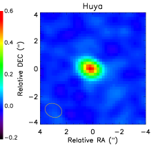
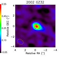
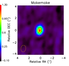
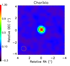
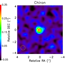
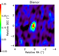
Figure 1: ALMA 233 GHz images of the six targets, combining the four spectral windows. The color bar indicates the flux scale (mJy/beam).

3 Modelling

The essential approach to determine the radio emissivity of the observed TNOs / Centaurs is to combine the modelling of their mm/submm flux with previous measurements from far-IR facilities, namely Spitzer, Herschel (and WISE if available). For most objects, in the absence of information on shape and/or rotational parameters (spin period and orientation), we performed standard NEATM (Near Earth Asteroid Standard Model) fits, assuming sphericity. For several objects, for which such information may be available, we explored more detailed thermophysical and non-spherical models. This is the case especially of Chariklo and Chiron, for which we also investigated the possible contribution of rings to the observed fluxes.

3.1 Spherical NEATM fits

We started with standard NEATM fits of the thermal data. In this approach (Harris, 1998), the thermal flux is calculated as the one resulting from instantaneous equilibrium of the object (assumed spherical) with solar insolation, but correcting the temperatures by a semi-empirical beaming factor $\eta$, a wavelength-independent quantity which phenomenologically describes the combined effects of thermal inertia, spin state, and surface roughness. The NEATM approach is suitable when multiple thermal wavelengths are available; in this case $\eta$ is, in essence, adjusted to match the object’s SED. The local temperature is then expressed as a function of solar zenith angle SZA:

$$T(SZA)=\left(\frac{S_{\odot}(1-p_{v}q)}{\eta\epsilon_{b}\leavevmode\nobreak\ r_{h}^{2}}\right)^{0.25}\leavevmode\nobreak\ cos^{0.25}(SZA)$$ (1)

where $S_{\odot}$ is the solar constant at 1 AU, $r_{h}$ is the heliocentric distance in AU, and $p_{v}$, $q$ and $\epsilon_{b}$ are the object’s geometrical albedo, phase integral, and bolometric emissivity, respectively. Within NEATM, multiple thermal measurements are combined with the H_v magnitude to determine the object’s diameter, geometric albedo, and beaming factor. This still involves assumptions on $q$ and $\epsilon_{b}$. For TNOs, most models have used the $q$ vs $p_{v}$ dependence shown in Brucker et al. (2009) and a fixed $\epsilon_{b}$ of 0.9 or 0.95.

Table 2: Spherical NEATM fit results

Object	Diameter	Geometric	Beaming	Ref. for	Relative mm/submm
	(km)	albedo	factor	submm/mm data	emissivity
2002 GZ32	237${}_{-11}^{+12}$	0.036${}_{-0.005}^{+0.006}$	0.97${}_{-0.08}^{+0.07}$	This work	0.80${}_{-0.05}^{+0.05}$ (1.29 mm)
Bienor	199${}_{-12}^{+9}$	0.041${}_{-0.012}^{+0.016}$	1.58${}_{-0.11}^{+0.15}$	This work	0.62${}_{-0.07}^{+0.07}$ (1.29 mm)
Chariklo	241${}_{-8}^{+9}$	0.037${}_{-0.008}^{+0.009}$	1.20${}_{-0.08}^{+0.10}$	This work	1.25${}_{-0.10}^{+0.09}$ (1.29 mm)
				A01a	1.08${}_{-0.16}^{+0.16}$ (1.20 mm)
Chiron	210${}_{-14}^{+11}$	0.172${}_{-0.036}^{+0.043}$	0.93${}_{-0.10}^{+0.13}$	This work	0.63${}_{-0.07}^{+0.07}$ (1.29 mm)
				J92a	0.81${}_{-0.69}^{+0.56}$ (0.80 mm)
				A95a	0.55${}_{-0.13}^{+0.13}$ (1.20 mm)
Huya	458${}_{-21}^{+22}$	0.081${}_{-0.008}^{+0.008}$	0.93${}_{-0.08}^{+0.09}$	This work	0.73${}_{-0.10}^{+0.08}$ (1.29 mm)
2002 UX25 b	695${}_{-29}^{+30}$	0.104${}_{-0.010}^{+0.011}$	1.07${}_{-0.07}^{+0.10}$	BB17a	0.66${}_{-0.06}^{+0.05}$ (0.87 mm)
					0.65${}_{-0.05}^{+0.05}$ (1.30 mm)
Orcus b	960${}_{-42}^{+45}$	0.231${}_{-0.022}^{+0.017}$	0.97${}_{-0.13}^{+0.08}$	BB17a	0.75${}_{-0.07}^{+0.07}$ (0.87 mm)
					0.92${}_{-0.05}^{+0.07}$ (1.30 mm)
Quaoar b	1071${}_{-57}^{+53}$	0.124${}_{-0.012}^{+0.016}$	1.73${}_{-0.19}^{+0.16}$	BB17a	0.68${}_{-0.04}^{+0.05}$ (0.87 mm)
					0.46${}_{-0.03}^{+0.03}$ (1.30 mm)
Salacia b	909${}_{-38}^{+39}$	0.042${}_{-0.004}^{+0.004}$	1.15${}_{-0.08}^{+0.11}$	BB17a	0.62${}_{-0.04}^{+0.03}$ (0.87 mm)
					0.69${}_{-0.04}^{+0.03}$ (1.30 mm)
a A01:Altenhoff et al. (2001); BB17:Brown & Butler (2017); JL92:Jewitt & Luu (1992),
A95: Altenhoff & Stumpff (1995)
b Objects from Brown & Butler (2017)

Herschel data include PACS 3-band (70, 100, 160 $\mu$m) photometry for $\sim$120 objects and SPIRE (250, 350, 500 $\mu$m) 3-band photometry for a much more restricted sample ($\sim$10 objects). Out of the six objects in this study and the four objects observed by Brown & Butler (2017), eight (i.e. all except 2002 GZ₃₂ and Bienor) are part of the SPIRE sample. Nonetheless, based on Fornasier et al. (2013) who found that significant emissivity effects occur longwards of 200 $\mu$m, we did not include the SPIRE data when deriving the objects’ diameter, geometric albedo, and beaming factor. For this purpose, we used only the Spitzer, Herschel/PACS (and WISE) data, which were fit simultaneously – using the observing circumstances appropriate for each individual measurement – to derive the above three parameters. The flux measurements from ALMA and SPIRE were then fit to derive the relative spectral emissivity (i.e. $\epsilon_{\lambda}$ / $\epsilon_{b}$) at the corresponding wavelengths (Fig. 2). H_v magnitudes were taken from literature, normally sticking to the values used in the Herschel “TNOs are Cool” papers. For objects whose H_v magnitude is known to vary on orbital timescales (Chariklo, Chiron, and Bienor), we at this point simply used the H_v magnitude in the relevant time period (i.e. 2006-2010), noting that the inferred $p_{v}$ is of limited significance as being possibly affected by ring and/or dust contamination; specifically we used H_v = 7.30$\pm$0.2 for Chariklo, 5.92$\pm$0.2 for Chiron, and 7.57$\pm$0.34 for Bienor.

An important issue stressed by Brown & Butler (2017) is the need to evaluate realistic error bars on the fitted parameters. With respect to previous modelling of TNOs, their model included (a) a Monte Carlo Markov Chain (MCMC) approach (b) the inclusion of uncertainties on the input parameters $q$ (adopting a factor of 2 variability above and below the Brucker et al. (2009) relationship) and $\epsilon_{b}$ (considering the 0.80-1.00 range instead of a fixed value). For their four objects, they found somewhat different – and larger in average by 25 % – uncertainties compared to the results of Fornasier et al. (2013). Here, we kept the technical approach to error bars of Mueller et al. (2011) adopted in the series of “TNOs are Cool” papers, generating multiple datasets of synthetic fluxes to be fitted and of the input model parameters, based on the observational and model uncertainties. However, in addition to the uncertainty on H_v, we included uncertainties in $q$ and $\epsilon_{b}$, following Brown & Butler (2017). Consistent with these authors, we found that the latter, here implemented as a gaussian distribution of $\epsilon_{b}$ with mean and rms values of 0.90 and 0.06 respectively, has a significant impact on the range of solution parameters.

Spherical NEATM fits, including the retrieved emissivity curves, are gathered in Fig. 2, with solution parameters given in Table 2 for all our objects except Makemake – which is discussed separately below. We also include our solution fits of the data presented in Brown & Butler (2017), mainly to verify the consistency of our approach to theirs. In particular, allowing for the uncertainty in the bolometric emissivity, we redetermine the equivalent diameters of 2002 UX₂₅, Orcus, Quaoar and Salacia as 695${}_{-29}^{+30}$ km, 960${}_{-42}^{+45}$ km, 1071${}_{-57}^{+53}$ km and 909${}_{-38}^{+39}$ km, respectively, to be compared with 698$\pm$40 km, 965$\pm$40 km, 1083$\pm$50 km and 914$\pm$39 km in Brown & Butler (2017). Except for 2002 UX₂₅, for which our error bar is 25 % smaller than theirs, all diameter central values and uncertainties are fully consistent. We are unsure of the reason for the slightly discrepant result on the diameter uncertainty for 2002 UX₂₅, but feel that the difference should not be overstated, as the resulting error on the density would be only 13.5 % if our error on the diameter is adopted, vs 18.2 % for the value of Brown & Butler (2017). In any case, our results on the mm/submm emissivity of the four objects, shown in the insets Fig. 2, also show excellent consistency with Brown & Butler (2017) (see their Fig. 6).

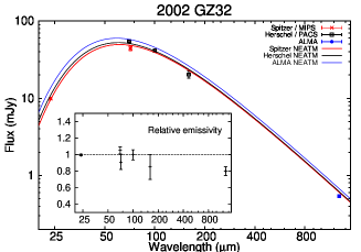
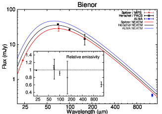
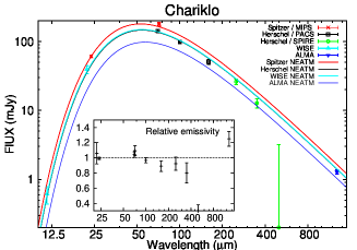
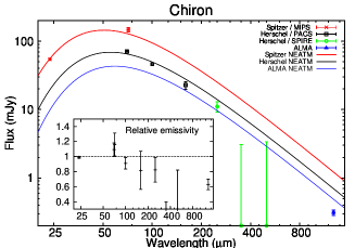
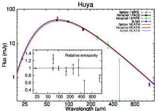
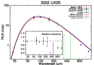
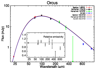
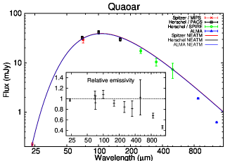
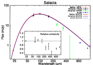
Figure 2: Flux measurements, spectral energy distribution and relative emissivity spectra (in inset) for nine TNOs, including the four objects from Brown & Butler (2017). Different colors show NEATM fits applied to the conditions of the different observations (Spitzer, Herschel, ALMA and WISE).

Prior to our ALMA measurements, two observations of Chiron (Jewitt & Luu, 1992; Altenhoff & Stumpff, 1995, using the JCMT and IRAM-30m, respectively) and one of Chariklo (Altenhoff et al., 2001, using IRAM-30m) had been acquired at mm/submm wavelengths, respectively in 1991, 1994 and 1999-2000. Observing parameters (geocentric and heliocentric distances) and fluxes can be found in these papers as well as in Groussin et al. (2004). We apply our NEATM fit solution parameters to these observations to obtain additional determinations of their mm/submm emissivity. Results are included in Table 2. In spite of vastly different observational distances (e.g. Chiron was at $\sim$ 10.5-8 AU in 1991-1994 vs $\sim$18.5 AU in 2016, and Chariklo was at $\sim$13 AU in 1999-2000 vs 15.5 AU in 2016), these earlier measurements are nicely consistent with the emissivities estimated from ALMA.

Of the nine objects presented in Fig. 2 and Table 2, eight clearly show relative emissivities lower than unity. With an emissivity of 1.25${}_{-0.10}^{+0.09}$ derived in this model from the ALMA data, Chariklo seems to be an outlier. As we show in the next section, however, this apparently anomalous emissivity can result from several factors that we will now study.

Table 3: Additional thermal modelling fit results: Chariklo

Object	Model	Diameter or	Geometric	Beaming	Thermal	Ref. for	Relative submm
		a,b,c (km)	albedo	factor	inertia (MKS)	submm/mm data	emissivity
Chariklo	TPMa, no rough.	240${}_{-8}^{+11}$	0.037${}_{-0.008}^{+0.007}$	N/A	2.6${}_{-1.4}^{+1.7}$	This work	1.24${}_{-0.09}^{+0.10}$ (1.29 mm)
Chariklo	TPMa, small rough.	240${}_{-8}^{+11}$	0.037${}_{-0.008}^{+0.007}$	N/A	4.3${}_{-1.4}^{+1.6}$	This work	1.23${}_{-0.10}^{+0.10}$ (1.29 mm)
Chariklo	TPMa, interm. rough.	240${}_{-8}^{+11}$	0.037${}_{-0.008}^{+0.007}$	N/A	5.9${}_{-1.8}^{+1.5}$	This work	1.22${}_{-0.10}^{+0.10}$ (1.29 mm)
Chariklo	TPMa, large rough.	240${}_{-8}^{+11}$	0.037${}_{-0.008}^{+0.007}$	N/A	8.0${}_{-1.7}^{+2.0}$	This work	1.21${}_{-0.10}^{+0.10}$ (1.29 mm)
Chariklo	NEATM, Maclaurin	143 x 143 x 96	0.038	1.09${}_{-0.07}^{+0.07}$	N/A	This work	1.00${}_{-0.07}^{+0.07}$ (1.29 mm)
						A01b	0.81${}_{-0.11}^{+0.14}$ (1.20 mm)
Chariklo	NEATM, Jacobi	160 x 142 x 88	0.041	1.04${}_{-0.07}^{+0.08}$	N/A	This work	0.92${}_{-0.06}^{+0.07}$ (1.29 mm)
						A01b	0.76${}_{-0.12}^{+0.11}$ (1.20 mm)
Chariklo	NEATM, Triaxial	146 x 131 x 101	0.038	1.11${}_{-0.09}^{+0.08}$	N/A	This work	1.06${}_{-0.08}^{+0.07}$ (1.29 mm)
						A01b	0.87${}_{-0.14}^{+0.14}$ (1.20 mm)
Chariklo, ring-corr.	NEATM	230${}_{-9}^{+8}$	0.040${}_{-0.008}^{+0.008}$	1.15${}_{-0.10}^{+0.08}$	N/A	This work	1.21${}_{-0.10}^{+0.10}$ (1.29 mm)
						A01b	1.01${}_{-0.17}^{+0.18}$ (1.20 mm)
Chariklo, ring-corr.	NEATM, Jacobi	154 x 136 x 84	0.041	1.00${}_{-0.08}^{+0.07}$	N/A	This work	0.89${}_{-0.08}^{+0.07}$ (1.29 mm)
						A01b	0.71${}_{-0.11}^{+0.13}$ (1.20 mm)
a TPM: thermophysical model
b A01:Altenhoff et al. (2001)

3.2 Chariklo: more detailed modelling

On June 3, 2013, observation of a stellar occultation by Chariklo resulted in the discovery of rings around the body (Braga-Ribas et al., 2014) and in bringing entirely new information on its shape. In addition to their huge significance in itself, this observation adds valuable constraints here, making possible a more detailed modelling of the object’s thermal flux. Indeed (i) the ring orientation provides information on Chariklo’s spin direction (ii) information on Chariklo’s shape permits us to consider non-spherical models and (iii) based on the rings physical characteristics deduced from the occultation, we can estimate their thermal emission.

3.2.1 Thermophysical model

Braga-Ribas et al. (2014) report the pole orientation of Chariklo’s ring system to be given by J2000 $\alpha_{P}$ = 151.30^∘$\pm$0.49^∘, $\delta_{P}$ = 41.48^∘$\pm$0.21^∘. A reasonable assumption is that the body’s pole orientation coincides with the ring pole orientation. Under this assumption, Chariklo’s sub-solar and sub-earth latitudes are approximately 0^∘ in early 1980 and late 2007, and reach extremal values of –58^∘ in mid-1996 and +58^∘ in late 2021. The sub-solar latitude was in the range –12^∘ to +14^∘ for the WISE, Spitzer and Herschel observations in 2006-2010, but reached +45^∘ in 2016 for the ALMA observations. Using this knowledge, along with Chariklo’s rotation period (7.004$\pm$0.036h; Fornasier et al., 2014), we fit the WISE, Spitzer and Herschel data with a spherical thermophysical model (TPM), accounting for the proper sub-solar/sub-earth latitude for each data set. The model free parameters are the equivalent diameter, geometric albedo, and now the thermal inertia ($\Gamma$). As there is a known degeneracy between thermal inertia and surface roughness, we specify four levels of roughness (“none”, “small”, “intermediate”, ”large”), and incorporate the effect of roughness as a ‘̀‘thermophysical model beaming factor” $\eta_{TPM}(\Theta)$, which for a given roughness scenario is a single-valued function of the thermal parameter (see discussion and Fig. 6 in Lellouch et al., 2011). Once the solution thermal inertia is found, the model is applied to the ALMA data, again with its proper sub-solar/sub-earth latitude. Within this framework, solutions for the diameter and geometric albedo (see Table 3) are virtually identical to those obtained from NEATM, and thermal inertias of 2.5–8 MKS are found. The apparent mm relative emissivity from the ALMA data is now nominally 1.23, instead of 1.25 from NEATM. A lower value is to be expected in relation to the more poleward sub-solar latitude in 2016 (causing the object to be in average warmer) than in 2006-2010, but the effect is very small, given the weak ($\sim$ linear) dependence of the mm flux to temperatures. Applying similarly the thermophysical model solutions to the IRAM observations of Altenhoff et al. (2001) leads to emissivity values that are insignificantly different from that obtained with NEATM (1.07$\pm$0.16 instead of 1.08$\pm$0.16, not detailed in Table 3).

3.2.2 Shape effects

Four additional multi-chord occultations by Chariklo were observed in April 29, 2014, June 28 2014, August 8, 2016 and October 1, 2016. Combining these data with those from June 2013, and using the pole orientation given by the rings, Leiva et al. (2017) estimated Chariklo’s size, shape and density. For this, they considered a variety of models, including two hydrostatic equilibrium models (Maclaurin spheroid and Jacobi ellipsoid), and a more generic triaxial ellipsoid shape in which the hydrostatic constraint was relaxed. Best fit solutions are: (i) Maclaurin spheroid: equatorial radius, a = b = 143${}^{+3}_{-6}$ km; polar radius, c = 96${}^{+14}_{-4}$ km; density = 970${}^{+300}_{-180}$ kg m^-3; (ii) Jacobi ellipsoid: semi-major axes, a = 157$\pm$4 km, b = 139$\pm$4 km, c = 86$\pm$1 km; density = 796${}^{+2}_{-4}$ kg m^-3 (these numbers override those given in Leiva et al. (2016) which did not include the occultations from 2016) (iii) triaxial ellipsoid: a = 148${}^{+6}_{-4}$ km, b = 132${}^{+6}_{-5}$ km, c = 102${}^{+10}_{-8}$ km. These non-spherical shapes lead to the object presenting a higher cross-section in 2016 vs 2006-2010, presumably contributing to the high apparent emissivity derived from ALMA. Below, we study this effect quantitatively.

Braga-Ribas et al. (2014); Duffard et al. (2014) and Fornasier et al. (2014) noted that the discovery of Chariklo’s rings provides a natural explanation of the brightness variability of the Chariklo+rings system, i.e. its fading from 1998 to 2009 and re-increase in brightness after that date. Fitting the H_v magnitude data with the sum of a spherical (or quasi-spherical in the case of Duffard et al., 2014) body with a ring of known dimensions but with changing aspect, they determined a ring albedo (I/F reflectivity) of $\sim$9 %, noting that the variations of the projected area of the object with season would also contribute to the secular variation of Chariklo’s H_v magnitude, thereby reducing the required ring albedo.

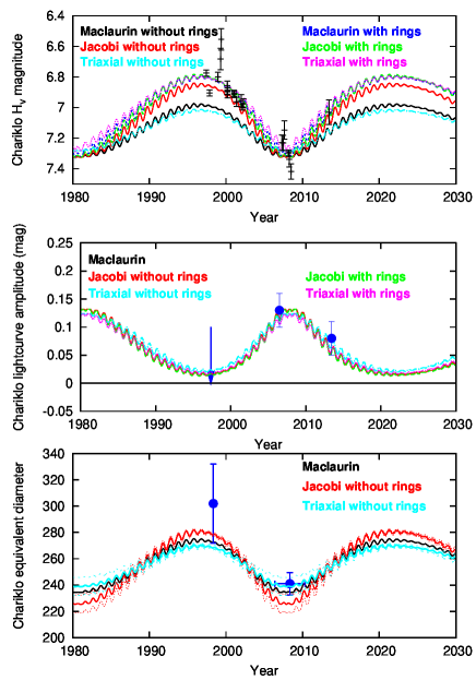
Figure 3: Models of: (top) H_v magnitude; (middle) optical lightcurve amplitude; and (iii) apparent diameter of Chariklo for the three shape models (Mclaurin spheroid, Jacobi ellipsoid, and generic triaxial ellipsoid) of Leiva et al. (2017). In the top panel, photometric data are from Fornasier et al. (2014). For the two ellipsoid cases, the model H_v is the mean value over the lightcurve. In the middle panel, lightcurves amplitudes $\Delta m$ = 0.13$\pm$0.03 and 0.08$\pm$0.03 mag in 2006 and 2013 (Galiazzo et al., 2016; Fornasier et al., 2014) and an upper limit ($\Delta m$ $\lessapprox$0.1 mag) in 1997 (Davies et al., 1998) are shown; the spheroid model does not produce any lightcurve. In the bottom panel, the diameter reported by Jewitt & Kalas (1998) for 1998 and in this work for 2006-2010 (Spitzer, WISE, Herschel) are shown (an additional measurement from WISE in 2010– Bauer et al., 2013, –giving D = 226.1$\pm$29.3 km, is not reported for plotting clarity). For the two ellipsoid cases, the apparent diameter is calculated at lightcurve maximum and minimum (dotted lines) and at the intermediate phase (solid lines). No contribution of Chariklo’s rings to the thermal emission is assumed here.

We briefly reconsidered these models by including the above three shape models from Leiva et al. (2017). As in the above papers, the adjustable parameters are Chariklo’s geometric albedo $p_{v}$ and the ring I/F reflectivity. As in Braga-Ribas et al. (2014) and Leiva et al. (2017), but unlike in Duffard et al. (2014) and Fornasier et al. (2014), we only included the contribution from Chariklo’s inner ring (C1R, radius 391 km, optical depth $\tau$=0.4), as the outer ring (C2R, radius 405 km, optical depth $\tau$=0.06) is $\sim$7 times optically thinner and likely has a negligible contribution to the system H_v magnitude. For the three shape models, Fig. 3 compares the calculated (i) H_v magnitude; (ii) lightcurve amplitude; and (iii) surface-equivalent diameter of the solid body, as a function of time, with relevant data. As Chariklo’s rotational period is not known with sufficient accuracy to rephase optical or thermal measurements, we calculate a mean H_v magnitude over the lightcurve in the case of the two ellipsoid models, while the equivalent diameter is calculated at maximum, minimum and intermediate phases. For the Maclaurin (resp. Jacobi, generic triaxial) model, the solution parameters are $p_{v}$= 0.038 (resp. 0.041, 0.038) and (I/F)_ring = 0.030 (resp. 0.010, resp. 0.035). Thus, as mentioned by Leiva et al. (2017) who derived very similar numbers, the ring contribution is vastly subdued when the object’s non-sphericity is taken into account. The Jacobi and generic triaxial shapes additionally predict a large variability of the optical lightcurve amplitude; this agrees with the detection of the optical lightcurve in 2006 and 2013 (Galiazzo et al., 2016; Fornasier et al., 2014) but not in 1997 (Davies et al., 1998). Finally, for all three models, the variation of the projected area with time is qualitatively consistent with the report of a significantly larger apparent diameter (302$\pm$30 km) in 1998 (Jewitt & Kalas, 1998) than in 2006-2010 (241$\pm 9$ km; see Table 2); this is explored more quantitatively in the next paragraph.

With these results in mind, we re-fitted the Chariklo thermal data with non-spherical models. Since the thermophysical models lead to very similar emissivity results as the NEATM, we mostly explored the effect of non-sphericity in NEATM, the difference between an “elliptic NEATM” and the standard NEATM being in the expression of the solar zenith angle at the surface of the ellipsoid, as well of course as the variability of the projected area in the former. The effect of ellipsoidal geometry in standard asteroid radiometric models has been first studied by Brown (1985). Specifying as input the three above shape models from Leiva et al. (2017), the WISE, Spitzer and Herschel data were refit in terms of (i) the beaming factor $\eta$ (ii) a scaling factor ($f_{scale}$) to the overall object dimensions. Chariklo’s geometric albedo was held fixed at the value determined previously for each shape model. The model was run for an intermediate phase between lightcurve maximum and minimum. Applying the model to the mm fluxes (ALMA, IRAM) then provided the radio emissivity. Uncertainty in the observed fluxes and other input parameters (H_v, $\epsilon_{b}$, $q$) were handled as before. Results are summarized in Table 3. For all three shape models, the scaling factor is very close to unity ($f_{scale}$ = 1.00$\pm$0.04 for the Maclaurin model, 1.02$\pm$0.04 for the Jacobi ellipsoid model, and 0.99$\pm$0.04 for the generic triaxial model), confirming the consistency of the occultation-determined sizes with thermal radiometry. The beaming factors are slightly smaller (nominally 1.04–1.11) than in the spherical NEATM, in accordance with the study of Brown (1985). The most important result for our purpose is that for these non-spherical models, the inferred relative radio emissivities have decreased in most cases to values less than 1 ($\sim$0.92-1.05 from ALMA and $\sim$0.76-0.87 from IRAM), demonstrating that for both the ALMA (March 2016) and IRAM (1999-2000) data, the “anomalously large” flux likely results from the large apparent cross section of Chariklo at those times (sub-solar/sub-earth latitude $\beta$$\sim$46^∘ in 2016 and -50^∘ in 1999-2000 vs $\beta$ = -12^∘ to 14^∘ over 2006-2010). Applying also the models to the conditions of the Jewitt & Kalas (1998) 20.3 $\mu$m measurements, we calculate fluxes of 58$\pm$2 mJy, 70$\pm$2 mJy, and 52$\pm$2 mJy for the Maclaurin, Jacobi, and generic triaxial models, respectively. All of these values agree reasonably well with the measured flux (66$\pm$12 mJy), albeit notably less so for the triaxial shape than for the Jacobi. In contrast, with the spherical NEATM solution (Table 2), the calculated 20.3 $\mu$m flux is only 34$\pm$1.5 mJy, at odds with the observations. All this clearly favors non-spherical over spherical models. Although Leiva et al. (2017) favored the generic triaxial shape as permitting to avoid an extremely low ($\lesssim$ 1 %) ring I/F, we prefer here the Jacobi ellipsoid as providing the best agreement to the Jewitt & Kalas (1998) flux; in what follows, this shape model is adopted.

3.2.3 Ring emission

We constructed a simple model to estimate the thermal emission from Chariklo’s rings. The model is based on a simplified version of Saturn’s rings models developed by Froidevaux (1981); Ferrari et al. (2005); Flandes et al. (2010). Direct absorbed radiation from the Sun $F_{abs}$ is the only considered source of energy for ring particles, i.e. we neglect heat sources due to thermal emission and reflected solar light from Chariklo itself, as well as mutual heating between ring particles. Under this assumption, the ring particle temperature $T_{P}$ will satisfy the following energy balance equation:

$$F_{abs}=\epsilon_{r,b}\leavevmode\nobreak\ \sigma\leavevmode\nobreak\ f\leavevmode\nobreak\ T_{P}^{4}\leavevmode\nobreak\ (1-\frac{\Omega_{P}}{4\pi})$$ (2)

where

$$F_{abs}=(1-A_{r})\leavevmode\nobreak\ C(B^{\prime},\tau)\leavevmode\nobreak\ \frac{S_{\odot}}{r_{h}^{2}}$$ (3)

Here $A_{r}$ is the Bond albedo of the ring particles and $\epsilon_{r,b}$ is their bolometric emissivity. $C$ is the ring shadowing function (i.e. the non-shadowed fractional area of a ring particle), which depends on the ring optical depth $\tau$ and the solar elevation above ring plane, $B^{\prime}$. ${\Omega_{P}}$ represents the angle subtended by neighboring particles, and can be expressed as ${\Omega_{P}}$ = 6 (1 - e^-τ) (Ferrari et al., 2005). Finally $f$ is the rotation rate factor of the particles; following Flandes et al. (2010), we considered slow rotators, i.e. $f$ = 2. For the ring shadowing function, we adopted the approximate expression from Altobelli et al. (2008):

$$C(B^{\prime},\tau)=\frac{sin\leavevmode\nobreak\ B^{\prime}}{1-e^{-\tau}}\leavevmode\nobreak\ (1-e^{-\tau/B^{\prime}})$$ (4)

Once the ring particle temperature $T_{P}$ is calculated in this manner, the ring radiance B_λ at wavelength $\lambda$ as seen from Earth and the associated brightness temperature $T_{B}(\lambda)$ are obtained as:

$$\textrm{B}_{\lambda}(T_{B}(\lambda))\leavevmode\nobreak\ =\leavevmode\nobreak\ \epsilon_{r,\lambda}\leavevmode\nobreak\ (1-e^{-\tau})\leavevmode\nobreak\ C({B},\tau)\leavevmode\nobreak\ \frac{\textrm{B}_{\lambda}(T_{P})}{sin\leavevmode\nobreak\ {B}}$$ (5)

where B_λ is the Planck function, $\epsilon_{r,\lambda}$ is the ring particle emissivity at wavelength $\lambda$, $B$ is the elevation of the observer above ring plane and $C(B,\tau)$ is the fractional emitting area of a ring particle as seen from elevation $B$ (Ferrari et al., 2005). Equation 5 reduces to B${}_{\lambda}(T_{B}(\lambda))$   = $\epsilon_{r,\lambda}$   (1 - e^-τ/B) B${}_{\lambda}(T_{P})$.

In the above model, we nominally assumed $\epsilon_{r,b}$ = $\epsilon_{r,\lambda}$ = 1. This likely provides an upper limit of the ring emission at the longest wavelengths. Specifically, Cassini/CIRS measurements of Saturn’s rings indicate that $\epsilon_{r,\lambda}$ declines at $\lambda$ longwards of $\sim$200 $\mu$m, in relation to the progressive increase in single scattering albedo of water ice particles (Spilker et al., 2005). Similarly, 1.3-3 mm observations of Saturn’s B-ring at high solar elevation indicate brightness temperatures of 15-30 K (Dunn et al., 2005), vs $\sim$90 K as measured by Cassini/CIRS shortwards of $\sim$200 $\mu$m (Spilker et al., 2005). Duffard et al. (2014) infer the presence of water ice in Chariklo’s rings. This might be taken as an argument that a similar roll-off in brightness temperature with increasing wavelengths occurs for Chariklo’s rings as well. We note however, that the albedo inferred above for Chariklo rings (I/F = 0.010-0.035) is much weaker than Saturn’s rings (I/F $\sim$ 0.3 – 0.7) and actually more similar to Uranus’ rings (I/F $\sim$ 0.05), which do not show evidence for water ice (de Kleer et al., 2013). Thus, water ice might be present in Chariklo’s rings only as a trace component. We note in passing that Duffard et al. (2014) base their argument for water ice on the detection of the 1.5 and 2.0 $\mu$m H₂O features in four spectra taken in 1997-2002 and again in 2013, but not in 2007-2008 when rings were edge-on. The identification of H₂O ice in 1997-2002 seems secure (see Guilbert-Lepoutre, 2011), but we feel that the single 2013 spectrum – which does not show directly the H₂O bands – is less convincing (1.3 $\sigma$ detection according to Table 2 of Duffard et al., 2014) and would deserve confirmation. If not present in Chariklo’s rings, an alternative explanation to the data could be that H₂O is located in restricted areas at high southern latitudes of Chariklo.

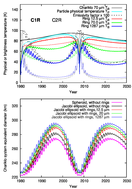
Figure 4: Thermal contribution of Chariklo rings. Top: Ring temperature model: Particle temperature (light blue) and ring brightness temperature at three wavelengths (red: 12.5 $\mu$m, green: 70 $\mu$m, dark blue: 1287 $\mu$m) as a function of time over 1980-2030 for Chariklo’s C1R $\tau$=0.4 (thick lines) and C2R $\tau$=0.06 (thin lines) rings. They are compared to the 70 $\mu$m brightness temperature of Chariklo itself (black). The dotted line represents the emissivity factor (1 - e^-τ/B), multiplied by 100. Bottom: Effect of rings on the apparent diameter. See text for details.

Model results in terms of ring particle physical temperature and ring brightness temperature at three wavelengths (12.5, 70 and 1287 $\mu$m) are shown in Fig. 4 for Chariklo’s C1R (thick lines) and C2R (thin lines) rings, and compared to the mean brightness temperature $T_{B,Ch}$ of Chariklo itself. The latter, which was calculated for the spherical NEATM solution ($\eta$=1.20, p_v = 0.036), is slightly wavelength-dependent and is here shown at 70 $\mu$m. Ring particle temperatures are colder than T_B,Ch due to ring low opacity and mutual shadowing. As expressed by Eq. 5, ring emission as seen from Earth is further reduced by a geometrical emissivity factor (1 - e^-τ/B), which is shown by the dotted lines in Fig. 4 (after multiplication by 100). Although this factor is wavelength-independent, it leads to a wavelength-dependent reduction of the ring $T_{B}$, as shown by the various curves in the top panel of Fig. 4.

The ring model was then used to calculate the flux emitted by the ring as a function of epoch and wavelength. To get a feeling about its significance, the ring flux was compared to the Chariklo flux calculated for the spherical NEATM solution, and then expressed in terms of a (wavelength-dependent) effective area, (i.e. the area that, with the same thermal properties as Chariklo itself, would produce a thermal flux equal to that of the rings). This effective area was then combined with the time-dependent projected area of Chariklo in the Jacobi ellipsoid model, and the result finally expressed in terms of the (epoch and wavelength-dependent) equivalent diameter for the Chariklo+rings system. Results are shown in the bottom panel of Fig. 4. We find that ring emission can bias the diameter measurement by up to $\sim$15 km (5 %) for wide open ring geometries. Although the ring $T_{B}$ decreases with increasing wavelength, the bias turns out to be more important at the longest wavelengths due to a Planck-function effect. This conclusion is however sensitive to our assumption that the long wavelength emission of Chariklo’s rings is not affected by scattering due to water ice.

With the above model, the contribution of Chariklo’s rings at the relevant epochs and wavelengths was subtracted from the thermal data, which were then refit with the spherical and elliptical NEATM models. The flux correction amounted to 1-10 % depending on each particular observation and generally increasing with wavelength. As detailed in Table 3, compared to the “no-ring” case, the ring correction leads to slightly smaller values for $\eta$ ($\sim$0.05), the equivalent diameter (by $\sim$5 %), and the relative emissivities (by $\sim$ 0.04). For the elliptical case, the best fit of the ring-corrected Chariklo thermal data is obtained for a scaling factor of 0.98$\pm$0.04 to the Jacobi ellipsoid model of Leiva et al. (2017), still fully consistent with that model.

Combining the effect of shape with the ring correction, we infer emissivities of 0.89$\pm$0.07 from our ALMA data and of 0.71$\pm$0.12 from the IRAM data. We did not explicitly run elliptic thermophysical models, but based on our analysis in section 3.2.1, the temperature effect associated to the more pole-on orientation in 2016 (ALMA) and 1999-2000 (IRAM) than in 2006-2010 causes an apparent $\sim$2 % increase in the emissivity. Correcting for this, we obtain our best estimate for the relative emissivity ($\epsilon_{\lambda}$ / $\epsilon_{b}$) as 0.87$\pm$0.07 from the ALMA data and 0.69$\pm$0.10 from IRAM. In summary, the above study shows that the apparent anomalous emissivity for Chariklo is the combined result of (i) change in the apparent cross section for an elliptical object (ii) change in the sub-solar latitude (iii) possible ring contribution, the first effect being by far the dominant one.

We estimate Chariklo’s ring thermal emission to be $\sim$0.13 mJy at 1287 $\mu$m (for 2016). While such a flux is not out of reach of ALMA in terms of sensitivity, the difficulty for detection is that the emission is azimuthally distributed, leading to very low surface brightnesses. Given also the proximity of the body at $\sim$30 milli-arcseconds, a direct imaging Chariklo’s rings with ALMA seems rather difficult.

In what follows, we apply the previous models for two other Centaurs, Chiron and Bienor, for which pole orientation parameters have been proposed (Ortiz et al., 2015; Fernández-Valenzuela et al., 2017).

Table 4: Additional thermal modelling fit results: Chiron and Bienor

Object	Model	Diameter or	Geometric	Beaming	Thermal	Ref. for	Relative submm
		a,b,c (km)	albedo	factor	inertia (MKS)	submm/mm data	emissivity
Chiron	TPMa, small rough.	214${}_{-7}^{+9}$	0.167${}_{-0.034}^{+0.024}$	N/A	0.7${}_{-0.7}^{+2.6}$	This work	0.62${}_{-0.06}^{+0.06}$ (1.29 mm)
Chiron	TPMa, interm. rough.	211${}_{-9}^{+11}$	0.171${}_{-0.032}^{+0.032}$	N/A	2.1${}_{-2.1}^{+3.6}$	This work	0.64${}_{-0.06}^{+0.06}$ (1.29 mm)
Chiron	TPMa, large rough.	210${}_{-12}^{+10}$	0.180${}_{-0.039}^{+0.037}$	N/A	4.9${}_{-3.3}^{+4.9}$	This work	0.65${}_{-0.07}^{+0.07}$ (1.29 mm)
Chiron	NEATM, elliptical	114 x 98 x 62	0.10	0.93${}_{-0.12}^{+0.12}$	N/A	This work	0.70${}^{+0.09}_{-0.08}$ (1.29 mm)
						A95b	0.56${}_{-0.13}^{+0.14}$ (1.20 mm)
Chiron, ring-corr.	NEATM	186${}_{-14}^{+13}$	0.100${}_{-0.021}^{+0.026}$	0.87${}_{-0.11}^{+0.15}$	N/A	This work	0.55${}_{-0.08}^{+0.09}$ (1.29 mm)
						A95b	0.41${}_{-0.14}^{+0.18}$ (1.20 mm)
Chiron, ring-corr.	NEATM, elliptical	100 x 86 x 54	0.13	0.84${}_{-0.10}^{+0.12}$	N/A	This work	0.62${}_{-0.09}^{+0.10}$ (1.29 mm)
						A95b	0.46${}_{-0.18}^{+0.17}$ (1.20 mm)
Chiron, ring-corr.c	NEATM, elliptical	100 x 86 x 54	0.13	0.84${}_{-0.10}^{+0.12}$	N/A	This work	0.87${}_{-0.13}^{+0.12}$ (1.29 mm)
Bienor	TPMa, no rough.	184${}_{-6}^{+6}$	0.050${}_{-0.016}^{+0.019}$	N/A	8${}_{-2}^{+3}$	This work	0.66${}_{-0.06}^{+0.07}$ (1.29 mm)
Bienor	TPMa, small rough.	182${}_{-7}^{+5}$	0.049${}_{-0.015}^{+0.016}$	N/A	10${}_{-3}^{+4}$	This work	0.67${}_{-0.07}^{+0.06}$ (1.29 mm)
Bienor	TPMa, interm. rough.	180${}_{-6}^{+6}$	0.050${}_{-0.013}^{+0.016}$	N/A	12${}_{-3}^{+4}$	This work	0.68${}_{-0.06}^{+0.06}$ (1.29 mm)
Bienor	TPMa, big rough.	179${}_{-7}^{+5}$	0.053${}_{-0.013}^{+0.018}$	N/A	15${}_{-4}^{+6}$	This work	0.68${}_{-0.06}^{+0.07}$ (1.29 mm)
Bienor	NEATM, elliptical	144 x 65 x 51	0.041	1.24$\pm$0.10	N/A	This work	0.64${}_{-0.07}^{+0.07}$ (1.29 mm)
a TPM: thermophysical model
b A95: Altenhoff & Stumpff (1995)
c In this case, the 1.29 mm flux is not corrected for a ring contribution, representing a case with extreme roll-off in brightness temperature
towards long wavelengths.

3.3 Chiron

Following the discovery of Chariklo’s rings, Ortiz et al. (2015) proposed that Chiron harbours a ring system as well. Their argumentation was based on (i) the evidence for absorption features in occultations observed in 1993, 1994 and 2011 (Bus et al., 1996; Elliot et al., 1995; Ruprecht et al., 2015) (ii) the time variability of Chiron’s H_v magnitude, optical lightcurve amplitude, and water ice spectral signature. Although the occultation features have been attributed before to a combination of narrow jets and a broader dust component, and the changing optical properties to photometric contamination by cometary-like activity, the general similarity of the widths, depths, and distance to the body of the occultation features with those of Chariklo led Ortiz et al. (2015) to favor the ring explanation, for which they determined a preferred pole orientation ($\lambda$ = 144^∘, $\beta$=24^∘, i.e. J2000 $\alpha_{P}$ = 156^∘, $\delta_{P}$ = 36^∘).

Although the radio-emissivity derived for Chiron from simple NEATM modelling does not show any “anomaly” (see Table 2), it is worth investigating the effects of pole orientation, shape and a possible ring system on the thermal photometry.

As for Chariklo, we assumed that the object’s pole orientation coincides with that of the proposed rings, and first ran a spherical thermophysical model, using a 5.92 hr rotation period. This led to best fit thermal inertias of 0.7 / 2.4 / 5.6 MKS for small / moderate / large roughness (no good fit was found without surface roughness), and to a relative radio emissivity of (0.62–0.65)$\pm$0.08, again insignificantly different from that obtained from spherical NEATM (0.63$\pm$0.07).

Shape information for Chiron is more uncertain than for Chariklo, given that none of the three occultations observed so far included multiple chords across the object . Assuming a Jacobi ellipsoid, a shape model can still be adopted based on other arguments. Following Luu & Jewitt (1990), Groussin et al. (2004) showed convincingly the anti-correlation of Chiron’s apparent lightcurve amplitude $\Delta m$ and apparent visible brightness and derived the true (i.e. body-only) lightcurve amplitude to be $\Delta m_{0}$ = 0.16$\pm$0.03. This is valid whether the “diluting factor” for the lightcurve amplitude is a coma or a ring system. In this latter case, and assuming identical pole orientation for the body and the ring system, $\Delta m_{0}$ occurs when the system is equator-on, implying $a$/$b$ = 1.16. Assuming the object to be a Jacobi figure in hydrostatic equilibrium, this implies also $c$/$a$ = 0.54. The spherical NEATM fit indicates an equivalent diameter D = 210 km (Table 2). Identifying the latter to 2 $a^{1/4}b^{1/4}c^{1/2}$ would lead to $a$ = 148 km, $b$ = 127 km, $c$ = 80 km. However, it can be anticipated that this initial guess is too large because, if the pole orientation proposed by Ortiz et al. (2015) is adopted, the geometry of the Spitzer/Herschel observations is considerably pole-on (sub-earth latitude $\beta$ $\sim$51-60^∘). Indeed, fitting these data with an elliptical NEATM model leads to a scaling factor $f_{scale}$ = 0.77$\pm$0.05 from the initial guess (i.e. best fit dimensions of 114 x 98 x 62 km) and a beaming factor $\eta$ = 0.93${}^{+0.10}_{-0.09}$. Running the model to the geometry of the mm observations then implies a relative emissivity of 0.56${}^{+0.14}_{-0.13}$ for the 1994 IRAM observations of Altenhoff & Stumpff (1995) and 0.70${}^{+0.09}_{-0.08}$ for our 2016 ALMA observations. These values are only marginally different from those inferred previously from the spherical NEATM model. This is because, with the assumed pole orientation, the projected areas at the epochs of the IRAM (sub-solar/sub-earth latitude $\beta$$\sim$-57^∘) and ALMA ($\beta$$\sim$+51^∘) data were similar to that at the Spitzer and Herschel epochs ($\beta$$\sim$51^∘ and $\beta$ $\sim$60^∘, respectively), a situation markedly different from the Chariklo case.

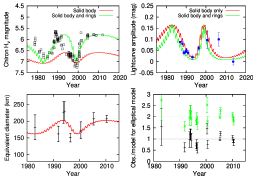
Figure 5: Models of: (top left) H_v magnitude; (top right) optical lightcurve amplitude and; (bottom left) apparent diameter of Chiron for a 114 x 98 x 62 km Jacobi ellipsoid with p_v = 0.10 and the orientation proposed by Ortiz et al. (2015). The modelled H_v and apparent diameter are calculated at a phase corresponding to mean lightcurve brightness. The first two panels include the effect of rings with a 20 % I/F reflectivity. In the top right panel, the blue symbols are the measurements as collected by Groussin et al. (2004), augmented by more recent measurements by Ortiz et al. (2015) and Galiazzo et al. (2016). In the bottom left panel, the model is compared to values of the diameter derived from our modelling of past thermal infrared observations (see Groussin et al., 2004). In the bottom right panel, the black points show ratios of individual measured thermal fluxes (some are shifted by $\pm$0.1 year for better visibility) by the elliptical NEATM model. In this panel, the green points (shifted by +1 in y) show the ratio of ring-corrected thermal fluxes by fluxes calculated from the elliptical model (see text for details).

Fig. 5 shows models of Chiron’s H_v magnitude, lightcurve amplitude, and equivalent diameter based on this Jacobi ellipsoid model. The large variations (up to 1.5 magnitude) of H_v cannot be fit with a realistic shape model, and require adjunction of a varying coma, a ring system, or more likely a combination of two (Ortiz et al., 2015), as the ring model fails to reproduce the evolution of H_v over 1987-1997. As done for Chariklo above, we fit the H_v data by the combination of the body and a ring system. We find a best-fit I/F of 0.20 for the rings, consistent with 0.17 from Ortiz et al. (2015), but stress that this is rather different from the I/F inferred above for Chariklo (I/F = 0.01-0.035), putting into question the similarity of Chiron’s putative ring system with Chariklo’s. We also note that with the rather elongated shape model we have adopted ($a$/$c$ = 1.85), the adjunction of a ring system has a relatively minor effect on the modelled lightcurve amplitude (top right panel of Fig. 5). Ortiz et al. (2015) further claimed that the presence of a ring system can explain the variability in the near-IR spectrum of Chiron, with the water ice spectral features being detected by Foster et al. (1999); Luu et al. (2000) in April 1998 and April 1999, but not by Romon-Martin et al. (2003) in June 2001. However, this argument is weak because with their preferred ring pole orientation, the sub-earth/solar latitude was approximately -9^∘ and +3^∘ for the first two spectra, vs +26^∘ for the last one, i.e. the rings were more edge-on when H₂O was detected than when it was not.

Numerous measurements of Chiron’s thermal flux and associated diameter have been obtained in the past. In the most detailed study before Spitzer/Herschel, Groussin et al. (2004) analyzed multiple-band ISOPHOT observations from 1996 with a spherical thermophysical model coupled with a standard beaming factor $\eta$ = 0.756. They inferred a diameter D = 142$\pm$10 km and a thermal inertia $\Gamma$ = 3${}^{+5}_{-3}$ MKS. On the basis of this model, they reanalyzed all anterior thermal flux measurements from Chiron, and noted a significant dispersion between the individually inferred diameters. Doing the same using our spherical NEATM results (i.e. fixing $\eta$ to 0.93${}^{+0.13}_{-0.10}$, see Table 2) we obtain very similar diameters as Groussin et al. (2004). Part of the dispersion can be explained by an elliptical body, as can be seen in the bottom left panel of Fig. 5. However, as shown in the bottom right panel of Fig. 5, calculating individual fluxes with the elliptical NEATM solution applied to the condition of each observation still shows significant residuals from the observations, suggesting that additional factors come into play (presumably, measurement errors).

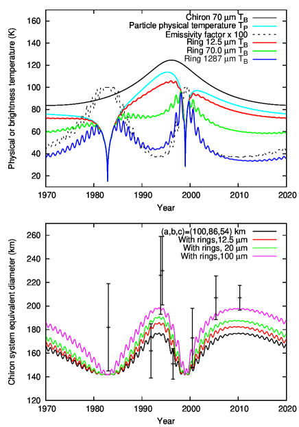
Figure 6: Thermal contribution of Chiron putative ring. Top: Ring temperature model: Particle temperature (light blue) and ring brightness temperature at three wavelengths (red: 12.5 $\mu$m, green: 70 $\mu$m, dark blue: 1287 $\mu$m) as a function of time over 1970-2020 for a Chiron ring with $\tau$=0.4. They are compared to the 70 $\mu$m brightness temperature of Chiron itself (black). The dotted line represents the emissivity factor (1 - e^-τ/B), multiplied by 100. Bottom: Wavelength-dependent effect of rings on the apparent diameter. See text for details.

We also applied the ring thermal model to the Chiron case. For this we used the ring parameters considered by Ortiz et al. (2015), i.e. a 324 km diameter, a 10 km width and a 0.4 opacity. Similar to Fig. 4, Fig. 6 shows (i) the ring particle physical temperature and ring brightness temperature vs time (top panel) and (ii) the putative effect of ring emission to the Chiron equivalent diameter. In this case, Chiron’s absolute dimensions were tuned so as to fit the smallest diameter determination (i.e., from Groussin et al. (2004) in 1996), multiplying the “no-ring” Jacobi ellipsoid solution by 0.875 (i.e., giving $a$ = 100 km, $b$ = 86 km, $c$ = 54 km) and increasing its geometric albedo to 0.13 to continue to match the H_v magnitude. These calculations qualitatively show that Chiron’s rings, if existent, would affect diameter determinations. However, Fig. 6 suggests that including the effect of Chiron’s rings does not permit to fully reconcile the discrepant diameter determinations; in particular, the ring contribution appears maximal over 1991–1995, yet diameter measurements over this period indicate large dispersions. We nonetheless explored this further by fitting thermal fluxes corrected by our estimates of the ring contribution. A spherical NEATM fit of the Herschel/Spitzer ring-corrected fluxes indicates a best-fit diameter of 186${}^{+13}_{-14}$ km and beaming factor $\eta$ = 0.87${}^{+0.15}_{-0.11}$. Using instead the elliptical model and starting from the 148 x 127 x 80 km initial guess model, we found a best fit scaling factor $f_{scale}$ = 0.69$\pm$ 0.05, giving nominally 102 x 87 x 55 km, and a beaming factor $\eta$ = 0.84${}^{+0.12}_{-0.10}$. For both cases, the associated radio emissivities, based either on our own data or on the Altenhoff & Stumpff (1995) data, are summarized in Table 4 . The above figures illustrate quantitatively the extent to which a ring system would affect the diameter determinations. However, applying this ring-corrected elliptical model to past (ring-corrected) thermal observations leads to observed/modelled residuals comparable to the “no-ring” case (compare green and black points in the bottom right panel of Fig. 5).

In summary, we feel that the case for a ring system around Chiron with properties similar to Chariklo’s remains doubtful in several aspects, and is not particularly supported by the overall analysis of the thermal data. In contrast, the characteristics and variability of Chiron’s optical lightcurve are consistent with a triaxial body in hydrostatic equilibrium. We thus do not adopt the “ring-corrected” emissivities, favoring instead values from the uncorrected elliptical NEATM, and finally obtaining a relative emissivity of 0.70$\pm$0.09 at 1.29 mm based on the ALMA flux measurement.

3.4 Bienor

Recently, Fernández-Valenzuela et al. (2017) presented time series photometry of (54598) Bienor over 2013-2016, and by comparison with earlier literature found a strong variation of both the lightcurve amplitude (from $\Delta m$$\sim$0.6 mag in 2000 to $\sim$0.1 mag currently) and the absolute magnitude (changing abruptly from H_v$\sim$8.1 in 2000 to H_v$\sim$7.4 in 2008 and beyond). Interpreting the lightcurve amplitude evolution as due to a change of the sub-observer latitude, they proposed a solution for the rotation axis ($\lambda$ = 35$\pm$8^∘, $\beta$=50$\pm$3^∘, i.e. J2000 $\alpha_{P}$ $\sim$ 4^∘, $\delta_{P}$ $\sim$ 58^∘) along with a shape model. Assuming hydrostatic equilibrium, the axis ratios are $b$/$a$ = 0.45$\pm$0.05 and $c$/$b$ = 0.79$\pm$0.02. Fernández-Valenzuela et al. (2017) however noted that this model does not simultaneously reproduce the H_v evolution and considered a variety of more complex models, such as non-hydrostatic equilibrium, a time-variable albedo, model including a ring contribution, etc. None of the models – except apparently the albedo model, but the latter is not really described – achieves a good fit of the H_v evolution (see Fig. 3 of Fernández-Valenzuela et al., 2017). We do not attempt here to interpret in detail the photometric behavior of Bienor, but note that it is reminiscent of that of (139775) 2001 QG₂₉₈, convincingly demonstrated to be a contact binary with changing viewing geometry (Lacerda, 2001).

Table 5: Makemake model fits

Model	Makemake			Moon			Dust			Relative submm
	D (km)	pv	$\eta$	D (km)	pv	$\eta$	Tdust (K)	Area (km2)	Mass (kg)	emissivity
Makemake alone	1430	0.795	2.0${}^{+0.75}_{-0.65}$	N/A	N/A	N/A	N/A	N/A	N/A	1.03${}^{+0.10}_{-0.09}$
Makemake + moon	1430	0.795	2.64	265${}^{+166}_{-193}$	0.017${}^{+0.21}_{-0.010}$	0.34${}^{+0.18}_{-0.27}$	N/A	N/A	N/A	1.05${}^{+0.10}_{-0.10}$
Makemake + dust	1430	0.795	2.23${}^{+0.76}_{-0.80}$	N/A	N/A	N/A	54.6	4.1$\times$105	7.2$\times$106	1.07${}^{+0.10}_{-0.09}$

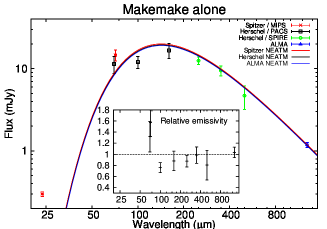
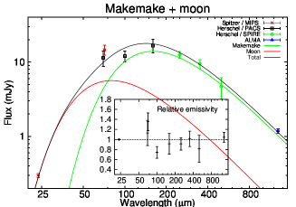
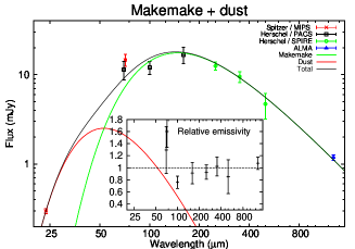
Figure 7: Flux measurements, spectral energy distribution and relative emissivity spectra (in inset) of Makemake, for the three considered models. Model fit parameters are as follows. (Left): “Makemake alone” model: D = 1430 km, p_v = 0.795, $\eta$ = 1.69. (Center): “Makemake + moon” model: For Makemake, D = 1430 km, p_v = 0.795, $\eta$ = 2.64; for the moon, D = 323 km, p_v = 0.012, $\eta$ = 0.406. (Right): “Makemake + dust” model: For Makemake, D = 1430 km, p_v = 0.795, $\eta$ = 1.95; for the dust, T = 54.6 K, mass = 7.2$\times$10⁹ kg. In the left panel, different colors show NEATM fits applied to the conditions of the different observations (Spitzer, Herschel, and ALMA). In the other two panels, the models are shown for the Herschel conditions.

Still, all models presented in Fernández-Valenzuela et al. (2017) call for generally similar pole orientations and shape models. We thus adopt the above solution parameters, and refit the Spitzer/Herschel thermal data with elliptical NEATM. Free parameters are a scaling factor to the shape model and the beaming factor (the albedo is kept at 0.041 from Table 2, which may not be accurate but is unimportant). The best fit solution is found for a = 144 km, b = 65 km and c = 51 km, with 4 % uncertainties, and $\eta$ = 1.24$\pm$0.10, noticeably different from the value obtained before from the spherical model (1.58${}^{+0.15}_{-0.11}$). With these values, the equivalent diameter of Bienor at the Spitzer (July 2014, sub-solar latitude $\beta$ = -29^∘) and Herschel (January 2011, $\beta$ = -49.5^∘) epochs is 158 and 177 km, respectively, considerably smaller than derived from the spherical model (199 km) and illustrating the limited value of a direct scaling of a shape model to a diameter determined from a spherical model. Nonetheless, applying the model to the geometry of the ALMA observations ($\beta$ = -58^∘) leads to a relative 1.29 mm emissivity of 0.64$\pm$0.07, virtually identical to the value from spherical NEATM (see Table 2).

Application of a spherical thermophysical model with the above orientation parameters, a rotational period of 9.17 hr (Fernández-Valenzuela et al., 2017), and various levels of roughness, leads to best fit thermal inertia of 8-15 MKS, a diameter of (179-184)$\pm$6 km, and a relative 1.29 mm emissivity of 0.68$\pm$0.07 (Table 4). Although the pole direction of Bienor remains to be confirmed, we adopt this as the best guess estimate of the object’s mm/submm emissivity.

We finally note that a stellar occultation by 2002 GZ₃₂ was successfully observed from several locations in Europe on May 20, 2017. When a shape model becomes available, this will provide the opportunity to reinterpret the thermal measurements, including our ALMA data.

3.5 Makemake

Before our measurement with ALMA, Makemake had been measured in the thermal range by Spitzer (Stansberry et al., 2008) and Herschel (Lim et al., 2010). As demonstrated at that time, standard NEATM fits fail to reproduce Makemake’s SED, and a multi-component model is required. Within NEATM, Lim et al. (2010) found solutions combining a large, high-albedo unit making up most of Makemake’s surface, and a localized, very dark unit, which is responsible for Makemake’s elevated 24 $\mu$m flux; in these models, the two units have very different values of the beaming factor ($\eta$= 1.3-2.2 and 0.4-0.5 respectively), suggesting sharply different thermal properties. Lim et al. (2010) further suggested that the dark terrain could represent a satellite, an hypothesis that gained credit with the discovery of S/2015 (136472)1 by Parker et al. (2016). These latter authors revisited the thermal models by including new constraints from (i) the H_V magnitude of the satellite, 7.80 mag fainter than Makemake and (ii) the occultation-derived diameter of Makemake (Ortiz et al., 2012; Brown, 2013b), confirming the essential conclusion that S/2015 (136472)1 may contribute a large fraction of the flux associated to the dark terrain. As noted by Parker et al. (2016), their models still do not fully reproduce the system 24 $\mu$m flux; yet they invoke $\eta$ values of 0.25-0.40. Such values are hard to understand physically, as even a surface saturated with hemispherical craters does not produce beaming factors lower than 0.6 (Spencer, 1990; Lellouch et al., 2013).

To determine the mm emissivity of Makemake in spite of these complications, we considered three end-member models, termed “Makemake-alone”, “Makemake + moon”, and “Makemake + dust”. In all cases, Makemake diameter and geometric albedo were held fixed at values determined from the stellar occultation. As a compromise between the (anyway similar) values given in Ortiz et al. (2012) and Brown (2013b), we adopted D = 1430 km, which for H_v = 0.091$\pm$0.015 (Parker et al., 2016), gives p_v = 0.795. As for the other objects, the models were applied to the set of Spitzer, Herschel, and ALMA fluxes. We used the Spitzer and Herschel/PACS flux values as published in Lim et al. (2010), but updated the Herschel/SPIRE fluxes, accounting for (i) a new reduction pipeline (HIPE version 8.2) and destriping methods (Fornasier et al., 2013) (ii) the availability of new Makemake observations from June 2010, in addition to the Nov./Dec. 2009 data presented in Lim et al. (2010). Averaging the two epochs, the new SPIRE fluxes are 12.5$\pm$1.3 mJy, 9.5$\pm$1.3 mJy, and 4.7$\pm$1.5 mJy at 250, 350 and 500 $\mu$m respectively.

In the first model (“Makemake-alone”), a standard NEATM fit was performed on the 3-band Herschel/PACS and the Spitzer 71.42 $\mu$m fluxes, ignoring the Spitzer 23.68 $\mu$m flux, with $\eta_{Make}$ as the only free parameter. As before, the model was then applied to other wavelengths to determine the corresponding spectral emissivities. The best fit solution, shown in the left panel of Fig.7, has $\eta_{Make}$ = 1.69, but even though the diameter and geometric albedos are fixed, the error bar on $\eta_{Make}$ is large ($\eta_{Make}$ = 2.0${}^{+0.75}_{-0.65}$; see Table 5), a consequence of the strong effect of the phase integral uncertainty for a bright object. Our ALMA flux measurements then implies a 1.03${}^{+0.10}_{-0.09}$ relative mm emissivity.

In a second model (“Makemake + moon”), the two Spitzer and the three Herschel/PACS measurements were fit with the sum of emission from Makemake and its moon. This model had initially four parameters, $\eta_{Make}$ and (D, p_v and $\eta$) for its moon, for which we adopted H_v = 7.89$\pm$0.3 (to allow for possible lightcurve variation). However, the system was somehow degenerate and best fit solutions tended to call for very large values of $\eta_{Make}$ ($>$3-4), while values larger than $\sim$2.7 are unphysical (see e.g. Fig. 4 of Lellouch et al., 2013). $\eta_{Make}$ was then fixed at a maximum value of 2.64. Even then, the problem remained somewhat under constrained, leading to broad ranges for (D, p_v and $\eta$) of the moon (Table 5). More worryingly but consistent with the previous studies (Lim et al., 2010; Parker et al., 2016), the solution range of $\eta_{moon}$ remained unphysical (0.34${}^{+0.18}_{-0.27}$) suggesting that Makemake’s moon alone might not entirely explain the 24-$\mu$m flux. Since the temperatures scale as ($\eta$$\epsilon_{b}$)^-1/4, a possible way to alleviate the problem would be to invoke a bolometric emissivity much lower than 1 for Makemake’s moon, but we note that restoring physically-reasonable values of $\eta$ (say $\eta$ $>$ 0.65) would then require $\epsilon_{b}$$<$0.5. In any case, with this “Makemake + moon” model, we infer a 1.05${}^{+0.10}_{-0.10}$ relative mm emissivity for the system.

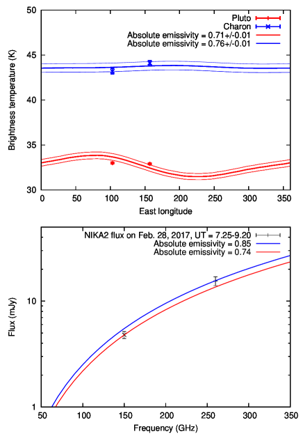
Figure 8: Top: Separate 0.86 mm brightness temperatures of Pluto and Charon measured by ALMA on June 12 and 13, 2015 (Butler et al., 2017), compared to calculations based on the Lellouch et al. (2016) model, and adjusting the absolute 0.86 mm emissivity to 0.71$\pm$0.01 for Pluto and 0.76$\pm$0.06 for Charon. Bottom: Flux density of the Pluto+Charon system for the conditions of the IRAM/NIKA2 observations of Feb. 28, 2017, and two values (0.72 and 0.85) of the system absolute emissivity. The statistical and calibration error bars have been combined quadratically.

In a third model, the 24 $\mu$m flux excess from Makemake’s system was attributed to dust emission. For this we adopted the dust absorption coefficients of Li and Draine (2001), giving e.g. $\kappa$ = 56 m² kg^-1 at 23.68 $\mu$m, and specified a dust grain temperature of 54.6 K, which corresponds to the instantaneous equilibrium of a sun-facing surface with zero albedo at Makemake’s 52 AU distance. This choice is somewhat arbitrary as small grains could be poor radiators (hence warmer than the above value), and/or radiating over 4$\pi$ (hence cooler). With these values, we infer an effective emitting area of 4.1x10⁵ km² for the grains, equivalent to a 720 km diameter, and a total dust mass of 7.2$\times$10⁶ kg. These figures do not seem unreasonable, although there is no evidence for dust activity at Makemake. Once corrected for the dust contribution at all wavelengths, the Spitzer and Herschel fluxes were refit with a Makemake model, again with $\eta_{Make}$ as the only free parameter, leading to a best fit value of $\eta_{Make}$ = 1.94 and a range of 2.23${}^{+0.76}_{-0.80}$. We note that significantly cooler grain temperatures than the above value would not permit to match the data. For example, assuming slowly rotating large dust grains (radiating over 2$\pi$), i.e. a grain temperature 2^1/4 lower (45.9 K) would require a total dust mass $\sim$8 times larger, but then the corrected fluxes would lead to an unphysical $\eta_{Make}$ = 3.7${}^{+1.2}_{-1.3}$.

While each of the three models had its own issues, they all lead to remarkably similar values of the relative mm emissivity, consistent with unity, as summarized in Table 5 and Fig. 7. Complications associated with non-spherical shape and/or with changing apparent orientations can be dismissed as (i) stellar occultation indicates that Makemake has a low oblateness (projected elongation $<$1.06; Ortiz et al., 2012; Brown, 2013b); and (ii) Makemake has travelled only 10^∘ along its orbit in the 2006-2016 timeframe covered by the thermal measurements, limiting changes in the sub-solar latitude to less than this value. We conclude that, unlike all other objects in our sample and that of Brown & Butler (2017), Makemake does have a relative mm emissivity close to 1. Interestingly, in spite of considerably larger error bars, the SPIRE fluxes are also consistent with a relative emissivity of 1 over 250-500 $\mu$m (see insets of Fig. 7).

Table 6: Pluto/Charon NEATM fits

Model	Diameter (km)		$p_{v}$		$\eta$		Relative submm
	Pluto	Charon	Pluto	Charon	Pluto	Charon	emissivity
1-component	2279${}^{+112}_{-108}$		0.66${}^{+0.12}_{-0.12}$		1.28${}^{+0.52}_{-0.70}$		0.99${}^{+0.05}_{-0.04}$ (0.86 mm)
2-component	2238${}^{+248}_{-190}$	1207	0.61${}^{+0.11}_{-0.13}$	0.362	2.62${}^{+1.51}_{-1.47}$	1.23${}^{+0.23}_{-0.17}$	0.88${}^{+0.06}_{-0.07}$ (0.86 mm)

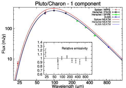
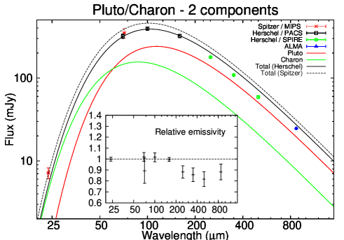
Figure 9: Flux measurements, spectral energy distribution and relative emissivity spectra (in inset) of the Pluto/Charon system, for the 1- and 2- component NEATM fits. (Left): 1-component fit, with following parameters: D = 2294 km, p_v = 0.64, $\eta$ = 1.38. (Right): 2-component fit, with fixed diameter/albedo for Charon. Model parameters are: Charon, D = 1207 km, p_v = 0.362, $\eta$ = 1.20; Pluto, D = 2225 km, p_v = 0.61, $\eta$ = 2.56. In the left panel, different colors show NEATM fits applied to the conditions of the different observations (Spitzer, Herschel, and ALMA). In the ring panel, the individual model Pluto (red) and Charon (green) components are shown for the Herschel conditions, and the total model flux (black) is shown both for Herschel (solid line) and Spitzer (dashed line).

3.6 Pluto and Charon

3.6.1 ALMA observations

The thermal emission from the Pluto/Charon system has been investigated in considerable details in the last 20 years. This includes spatially unresolved but rotationally repeated far-IR measurements (i.e. thermal lightcurves) using ISO, Spitzer and Herschel over 20-500 $\mu$m (Lellouch et al., 2000a, 2011, 2016) and numerous but more widespread ground-based mm/submm data. Initially, the latter did not resolve the Pluto/Charon system (see Lellouch et al., 2000b, and references therein), but the advent of interferometers (SMA, VLA, ALMA) permitted the thermal emission from Pluto and Charon to be measured separately (Gurwell, Butler & Moullet, 2011; Butler et al., 2015, 2017). In particular, based on ALMA observations acquired on June 12 and 13, 2015 (i.e. at two separate longitudes) which also led to the detection of CO and HCN in Pluto’s atmosphere (Lellouch et al., 2017), Butler et al. (2017) reported 860 $\mu$m brightness temperatures of $\sim$33 K for Pluto and $\sim$43.5 K for Charon, providing a definitive demonstration that Charon is warmer than Pluto. Making use of the multi-terrain thermophysical models presented by Lellouch et al. (2011, 2016), these measurements were interpreted in terms of separate absolute 860 $\mu$m emissivities of the two objects, found to be 0.69-0.72 for Pluto and 0.75-0.77 for Charon (Butler et al., 2017). Fits of the ALMA fluxes for the two observing dates are shown in the top panel of Fig.8. For a bolometric emissivity of 0.9, as is characteristic of the models of Lellouch et al. (2016), this implies relative emissivities of 0.78$\pm$0.015 and 0.84$\pm$0.01, respectively, i.e. a surface weighted-average value of 0.80 for the Pluto/Charon system.

As these values were obtained from a model that makes use of considerably more information (thermal lightcurves, precise object sizes, distribution of ices, etc.) than is available for other TNOs, it is enlightening to explore what could be derived on the mm emissivity of the Pluto system by applying a simple NEATM analysis as for other objects. For this purpose, we first created a Pluto/Charon dataset comparable to what we have for the other TNOs by averaging the Spitzer/MIPS fluxes (8 visits in 2004, sampling the Pluto lightcurve in 2004) and the Herschel/PACS and /SPIRE data (9 visits each in 2012). In doing so, the error bar on each flux value was defined by the (real) dispersion of the measurements at a given wavelength due to thermal lightcurve, rather than by the noise of each individual measurement. We then performed a simple NEATM analysis of the Spitzer, Herschel and ALMA fluxes, considering, as for Makemake, 1- and 2- components fits. Results and fits are summarized in Table 6 and Fig. 9. In the 1-component fit, the relative 860 $\mu$m emissivity of the Pluto/Charon system is close to 1, but the solution diameter (2280$\pm$110 km) is as much as $\sim$15 % smaller than the equivalent diameter of the Pluto-Charon system (2670 km), a problem already encountered by Mommert et al. (2012). The inability of the 1-component NEATM model to fit the SED of Pluto/Charon is related to the fact that the two bodies have comparable sizes, yet different albedos. In the 2-component model, Charon’s diameter and geometric albedo were held fixed at their observed values (D = 1207 km, p_v = 0.36), and the SED of the system was fit in terms of four parameters, $\eta_{Charon}$ and (D, p_v and $\eta$) for Pluto. In this case, the Pluto best fit diameter was found to be 2225 km. This is still 6 % smaller than the known Pluto diameter (2380 km) – one likely reason being that part of Pluto’s surface is covered by isothermal N₂-ice at $\sim$37.4 K, which contributes little to the dayside thermal emission at the shorter wavelengths – but error bars (Table 6) encompass the true value. Thus the introduction of Charon essentially reconciles the radiometric Pluto diameter with its established value. In this 2-component fit, the ALMA-derived relative emissivity for the Pluto/Charon system is 0.88${}^{+0.06}_{-0.07}$ at 860 $\mu$m. It is gratifying that even with this simple model, the emissivity is only 1-$\sigma$ different from that obtained using the more detailed thermophysical models.

3.6.2 IRAM/NIKA2 observations

Most recently, the Pluto system was observed during the commissioning of the new NIKA2 wide-field camera (6.5 arcminutes covered by 2900 detectors) dual-band (1.15 mm/2 mm) camera installed at the IRAM-30 m radio-telescope on Pico Veleta, Spain (Calvo et al., 2016). Observations were taken on Feb. 29, 2017, UT 7.25-9.20, corresponding to 1.44 hr on-source time an observing longitude L = 87$\pm$2. Although, unlike the SMA, VLA and ALMA observations of Butler et al. (2017), these do not resolve Pluto from Charon, they provide the first detection of the system at 2 mm. The 1.15 and 2 mm bands cover approximately $\sim$230-285 GHz and $\sim$125-175 GHz at mid-power, with effective frequencies of 150 and 260 GHz. The Pluto+Charon fluxes were reported to be 4.8$\pm$0.2$\pm$0.3 mJy at 2 mm and 15.1$\pm$1.0$\pm$1.1 mJy at 1.15 mm (Adam et al., 2017), where the first (second) error bar indicates the statistical (calibration) uncertainty. We combine quadratically these error bars.

Applying the thermophysical model of Lellouch et al. (2016) to the geometry of these observations, we find that the ALMA-derived model, which has a system-weighted absolute emissivity of 0.72, is fully consistent with the 2 mm flux but falls below the measured 1.15 mm flux by 1.5 $\sigma$. Fine tuning the model to the observations, optimal fits of the 2 mm and 1.15 mm fluxes are achieved for absolute emissivities of 0.74$\pm$0.06 and 0.85$\pm$0.07, respectively. In the submm range, Lellouch et al. (2016) found that the emissivity of the Pluto system decreases from $\sim$1 at 20-25 $\mu$m to $\sim$0.7 at 500 $\mu$m. This, and the fact that a non-monotonic variation of the emissivity over 0.86-1.15-2 mm does not seem plausible, makes us suspect that the 1.15 mm flux reported by Adam et al. (2017) is slightly overestimated. In this respect, an additional source of uncertainty is the yet unknown telescope/instrument gain response with elevation, that would affect the 260 GHz flux at low elevation, but not the 150 GHz flux (J.-F. Lestrade, priv. comm.), an issue that will be revisited when more observations of calibrators with NIKA2 are available. For the time being, the ALMA-derived separate emissivities and Pluto and Charon are retained.

3.7 Other objects

We finally briefly reconsidered a few additional mm/submm observations of TNOs/Centaurs from literature. Few of these measurements led to actual detections. Exceptions are Varuna (Jewitt, Aussel & Evans, 2001; Lellouch et al., 2002), 1999 TC₃₆ (Altenhoff et al., 2004, who also obtained upper limits on 6 other objects), and Eris (Bertoldi et al., 2006).

Varuna: We first focus on the case of Varuna for which the above two measurements at radio wavelengths provided best fit diameters of 900-1060 km, in sharp contrast with the Spitzer (500$\pm$100 km, Stansberry et al., 2008) and Spitzer/Herschel (668${}^{+154}_{-86}$ km, Lellouch et al., 2013) values. Performing the same NEATM analysis as for all the TNOs observed by ALMA, we find an updated diameter of 654${}^{+154}_{-102}$ km, but unphysical mm/submm emissivities of 2.49${}^{+1.24}_{-1.00}$ at 0.850 mm and 1.91${}^{+1.00}_{-0.82}$ at 1.20 mm, using the fluxes reported by Jewitt, Aussel & Evans (2001) and Lellouch et al. (2002). This indicates a gross inconsistency between the far-IR and mm/submm measurements.

Sicardy et al. (2010) reported on a stellar occultation by Varuna on February 19, 2010. This occultation, which was acquired

near maximum lightcurve of the object, provided one 1003 km long chord across the object – in itself sharply inconsistent with the spherical solution from Spitzer/Herschel – along with a non-detection just 225 km south of that chord. Although this is insufficient to determine a complete shape and orientation model, probability considerations indicate that the most likely figure of the object is strongly elongated, with $a$ $\sim$ 860 km and $c$ $\sim$375 km (Sicardy et al., 2010). Varuna is also characterized by a marked optical lightcurve ($\Delta$m = 0.42 mag, period = 6.344 hr). Assuming hydrostatic equilibrium and considering different surface optical properties and pole orientation, Lacerda and Jewitt (2007) constrained axis ratios to be in the range $b/a$ = 0.63-0.80 and $c/a$ = 0.45-0.52. We here adopt for definitiveness $a$ = 860 km, $b$ = 550 km, $c$ = 390 km (the lunar model and aspect angle = 75^∘ from Lacerda and Jewitt, 2007)), giving p_v = 0.048. As was done above for Chariklo and Chiron, we refitted the Spitzer/Herschel data allowing for an overall scaling factor $f_{scale}$ on this shape model. Assuming that all observations referred to an intermediate phase between lightcurve maximum and minimum, we inferred $f_{scale}$ = 0.60${}^{+0.14}_{-0.08}$ and $\eta$ = 2.0${}^{+1.0}_{-0.5}$. The Spitzer data for Varuna include two epochs while the Herschel data correspond to yet another epoch. Even if all three epochs corresponded to lightcurve minimum, the required scaling factor would still be only 0.68${}^{+0.14}_{-0.08}$, grossly inconsistent with $f_{scale}$ = 1.

In contrast, the mm/submm measurements of Jewitt, Aussel & Evans (2001) and Lellouch et al. (2002), appear consistent with the above shape model. We fitted them separately (i.e. not including the Spitzer/Herschel data), assuming that they sample rotationally-averaged conditions, and adopting a beaming factor $\eta$ = 1.175$\pm$0.42. This number comes from fitting a gaussian distribution to the 85 beaming factor values reported by Lellouch et al. (2013) – and is similar to the “canonical” 1.20$\pm$0.35 value from Stansberry et al. (2008). A bolometric emissivity of 0.90$\pm$0.10 was still specified. These assumptions lead to relative emissivities of 0.81$\pm$0.23 and 0.62$\pm$0.23 at 0.85 and 1.20 mm, in full agreement with the values derived for other objects. It thus appears that the $\sim$3$\sigma$ detections reported by Jewitt, Aussel & Evans (2001) and Lellouch et al. (2002) were likely to be real, although we regard these derived emissivity values as tentative. The inconsistency between the occultation-derived size and the far-IR thermal measurements remains to be elucidated; for this a more detailed shape model from future stellar occultations will be welcome.

1999 TC₃₆: From stacking of IRAM observations gathered over Dec. 2000 – Mar. 2003 ($\sim$4 h integration total), Altenhoff et al. (2004) reported the detection of 1999TC₃₆ with a 1.11$\pm$0.26 mJy flux at 250 GHz. Their inferred diameter was 609${}^{+93}_{-47}$ km, largely inconsistent with the Spitzer/Herschel preferred solution (D = 393${}^{+25}_{-27}$ km, Mommert et al., 2012). Our joint NEATM analysis of the data would indeed lead to a similar D = 395${}^{+22}_{-31}$ km and an unphysical relative emissivity of 2.08${}^{+0.64}_{-0.49}$ at 250 GHz. 1999 TC₃₆ is a triple system (Benecchi et al., 2010) with rather similar relative sizes, estimated to $\sim$272, 251 km, and 132 km assuming equal albedos (Mommert et al., 2012). The largest two components (A1, A2) orbit each other with distance $a$ $\sim$ 867 km and period P $\sim$1.9 days. However the orbit orientation is such that they are not mutually eclipsing, and the overall photometric variability of the both the central pair (A1+A2) and of the third component (B) is small and shows no evidence for a lightcurve. Note also that 1999 TC₃₆ has traveled $\sim$22^∘ on its orbit over the entire time interval (Dec. 2000-July 2004-July 2010) covered by the thermal observations, restricted any changes of the sub-solar latitude to less than this number. All of this effectively rules out geometrical or orientation considerations as the cause of the discrepant far-IR and mm data. As the Spitzer and Herschel detections have high S/N (see Mommert et al., 2012), this suggests that the Altenhoff et al. (2004) detection might not be real. ALMA observations (resolving the system) should confirm the mm fluxes.

Eris was detected from IRAM in 2006 (Bertoldi et al., 2006) and later by Spitzer (Stansberry et al., 2008) and Herschel (Santos-Sanz et al., 2012; Lellouch et al., 2013). These data, along with the occultation results from Sicardy et al. (2011) are analyzed jointly by Kiss et al. (in prep.). Note also that new ALMA measurements of the Eris-Dysnomia system have become recently available (program 2015.1.00810.S, PI. M.E. Brown).

We note finally that Margot et al. (2002) reported a successful detection of 2002 AW₁₉₇ at 1.2 mm from IRAM and estimated a $\sim$890$\pm$120 km diameter, but did not quote the measured fluxes, which prevents us for performing a reanalysis.

4 Discussion and conclusions

Table 7: Emissivity correlation searches and statistics

Variables	Nvalues	$\rho$ 1	p 2
$\epsilon_{r}$ vs D	18	0.293	0.238 (1.2 $\sigma$)
$\epsilon_{r}$ vs pv	18	0.245	0.326 (1.0 $\sigma$)
$\epsilon_{r}$ vs $\eta$	18	-0.066	0.794 (0.3 $\sigma$)
$\epsilon_{r}$ vs TSS	18	0.009	0.971 (0.0 $\sigma$)
$\epsilon_{r}$ vs color	18	-0.287	0.249 (1.2 $\sigma$)
$\epsilon_{r}$ vs $f_{water}^{3}$	10	0.459	0.182 (1.4 $\sigma$)
1 $\rho$: Spearman rank correlation coefficient
2 p: significance p-value of correlation
3 H2O ice content, as defined by Brown, Schaller & Fraser (2012)

Wavelength	Nvalues	Median 1	Mean$\pm$stdev
0.87 mm	6	0.71${}^{+0.07}_{-0.01}$	0.72$\pm$0.08
1.3 mm	12	0.70${}^{+0.17}_{-0.16}$	0.73$\pm$0.15
Both	18	0.70${}^{+0.13}_{-0.13}$	0.73$\pm$0.13
1 Error bars encompass central 68.2 % of values

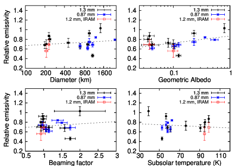
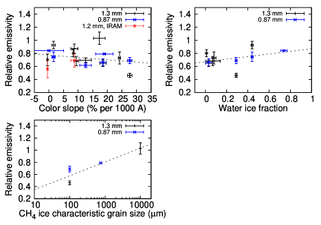
Figure 10: Derived radio emissivities plotted as a function of diameter, geometric albedo, beaming factor, sub-solar temperature, color slope, H₂O ice content, and CH₄ ice characteristic grain size (see text). Dashed lines indicate simple linear fits.

Including the two-wavelength measurements from Brown & Butler (2017) (4 objects, 8 measurements), and the values for Pluto and Charon based on the Butler et al. (2017) ALMA data – but not our more tentative inferences for Varuna – we now have radio (mm/submm) emissivities for 12 Centaurs/TNOs (18 independent values). Fig. 10 displays these emissivities as a function of conceivably relevant parameters, i.e. diameter, geometric albedo, beaming factor, sub-solar temperature as per the NEATM model, and color (i.e. the slope of the visible spectrum, taking values from (Lacerda et al., 2014)). These plots, along with a simple Spearman rank correlation analysis (Table 7), reveal no significant correlation of the emissivity with any of these five parameters, yet the dispersion exceeds individual error bars, suggesting real variability. Table 7 also summarizes statistics for the emissivities, considering either separately or together the 0.87 and 1.3 mm values. Noting that the dual-band emissivity measurements of Brown & Butler (2017) do not suggest any consistent emissivity trend with wavelength, we recommend using a $\epsilon_{r}$ = 0.70$\pm{0.13}$ median value for interpreting further measurements at mm/submm wavelengths.

Subdued emissivities at radio wavelengths are commonly measured in Solar System bodies, yet interpreted in various ways. For asteroids, absolute emissivities of 0.6-0.7 were reported (Redman et al., 1992; Müller & Lagerros, 1998). They were initially attributed to grain size dependent sub-surface scattering processes, but later shown to most likely result from a combination of surface roughness (differentially enhancing the short-wavelength fluxes), sub-surface sounding to deeper, colder temperatures relative to the dayside surface at the longest wavelengths, and specular reflection at surface with a moderate ($\sim$2.3) dielectric constant (Keihm et al., 2013). Radio-observations of cometary nuclei also indicate emissivities lower than 1, e.g. $\sim$0.5 for C1995 OI Hale-Bopp to reconcile sizes derived from IR and mm data (Fernández, 2002), and $<$0.8 (with 0.67 as the best guess value) for 8P/Tuttle (Boissier et al., 2011).

The NEATM (and thermophysical) model approaches we have used here implicitly define the emissivity in reference to the fluxes emitted from the surface itself. However, the analysis performed for Pluto/Charon by Lellouch et al. (2016, see their Table 2) indicates that for this system at least, allowing for the decrease of the dayside temperature in the sub-surface layers would lead to an increase of the emissivity by 1-4 % only at 500 $\mu$m (and beyond), even if the sub-diurnal layer is reached and its temperature affected by seasonal thermal inertia effects. A similar analysis cannot be done for the other objects under study here because we do not have a good handle on their individual thermal inertias. Still, the magnitude of the thermal gradient in the subsurface depends on (decreases with) the thermal inertia $\Gamma$ through the thermal parameter $\Theta=\frac{\Gamma\sqrt{\omega}}{\epsilon_{b}\sigma T_{ss}^{3}}$. TNOs as a population have thermal inertias of $\Gamma$ = (2.5$\pm$0.5) J m^-2s^-1/2K^-1 (Lellouch et al., 2013), i.e. 5-10 times less than Charon and Pluto, but this effect is largely compensated in the expression of $\Theta$ by a $\sim$20 times larger rotation rate $\omega$. Thus, although detailed calculations cannot be done, we suspect that sub-surface sounding is not the prime cause of the low radio emissivities. We also note that if it were the case, we might except a negative correlation of the radio emissivity with T_ss (for given values of $\Gamma$ and $\omega$, a higher T_ss corresponds to a lower $\Theta$, i.e. a larger thermal gradient in the subsurface, and thus a lower apparent emissivity if sub-surface sounding was the cause), and a positive correlation with the beaming factor $\eta$, which is a proxy for $\Theta$; those are not apparent in Fig. 10.

Dielectric reflection of the upward thermal radiation at the surface interface may contribute to the some of the depressed emissivities, but this effect is unlikely to be the dominant explanation. For example, a disk-averaged absolute radio emissivity of 0.54 ($\epsilon_{r}$ = 0.60) for a smooth surface implies a dielectric constant of $\sim$24, much higher than e.g. the value for solid organics ((1.2, Paillou et al., 2008) or H₂O ice ($\sim$3.1, ibid.). Although some materials have much higher dielectric constants, e.g. $\sim$25 for some iron oxides, this does not seem to be a realistic explanation. Applying the Ostro et al. (2009) relationship relating the dielectric constant and the near surface density $\rho$ would also lead to an unrealistic $\rho$ = 5.1 g cm^-3 density. Furthermore, the dielectric effect should be spectrally independent over the mm/submm range, unlike what is seen for Orcus and Quaoar in the Brown & Butler (2017) data.

The low emissivities observed here are reminiscent of similar findings on Giant Planet icy satellites, including (i) 3-40 mm brightness temperatures of Europa and especially Ganymede well below the subdiurnal temperatures (Muhleman & Berge, 1991) (ii) apparent emissivities of 0.4-0.9 in most of Saturn’s satellites at 2.2 cm (e.g. Ostro et al., 2006; Janssen et al., 2009; Le Gall et al., 2014; Ries & Janssen, 2015; Le Gall et al., 2017) as well as of composition and texture-dependent emissivities of ice and snow on Earth (Hewison & English, 1999). Scattering effects are usually invoked, either at the surface in presence of microscopic surface roughness, or, for transparent media, in volume, due to inhomogeneities or voids on scales comparable to $\lambda$.

Scattering effects are particle-size dependent, and produce emissivity minima for sizes $a$ $\sim$ $\lambda$/4$\pi$, i.e. $\sim$100 $\mu$m for $\lambda$ $\sim$1 mm. As was already mentioned in Lellouch et al. (2000b), this behavior was verified in models of terrestrial snow emissivity at 5-90 GHz as a function of particle size, absorption coefficients and medium density (Sherjal, 1995). These calculations are relevant for comparison with our measured emissivities because the absorption coefficient of ice at 260 K and 6 mm (50 GHz) is similar to that at 50 K and 1.2 mm (Mätzler, 1998; Lellouch et al., 2016). They indicate that for a snow density of 0.15-0.20, a minimum nadir emissivity of 0.65-0.70 is reached at $a$ $\sim$ $\lambda$/4$\pi$. Emissivity increases with increasing density, but low densities in upper surface layers are likely for TNOs, given that their low thermal inertia suggests considerable near-surface porosity (Lellouch et al., 2013; Ferrari & Lucas, 2016), and that the bulk density of TNOs smaller than $\sim$1000km is already significantly less than 1 (Brown, 2013a; Vilenius et al., 2014).

We speculate that part of the diversity we are seeing in TNO emissivity may be due to a variability in the mean particle size in the surface/upper sub-surface layers probed by the thermal radiation. Many KBOs show the spectral signatures of H₂O ice (Barucci et al., 2011; Brown, Schaller & Fraser, 2012). While spectra bear in principle information on particle size, the latter is generally hard to disentangle with effects due to H₂O abundance, geographical coverage and state of mixing (geographical vs intimate). For this reason, we classify our objects of interest according to the $f_{water}$ proxy defined by Brown, Schaller & Fraser (2012) for the overall “water ice amount” in the spectrum. Plotting the radio emissivities vs $f_{water}$ suggests (Fig. 10) a possible increase of $\epsilon_{r}$ with $f_{water}$, especially visible at 0.87 $\mu$m. The Spearman rank correlation coefficient and statistical significance are low (0.46 and 1.5$\sigma$, respectively) but still the strongest in Table 7. Thus, objects with the lowest radio emissivities may have effective particle sizes of $\sim$100 $\mu$m, and the positive correlation between $\epsilon_{r}$ with $f_{water}$, if real, could be explained if an increased $f_{water}$ traces an increase in particle size. As suggested by the last panel in Fig. 10, a similar correlation between grain size and radio emissivity – but restricted to three objects – may occur for the methane-rich bodies in our sample (Makemake, Pluto, Quaoar). Here we use CH₄ grain sizes of 1 cm for Makemake (Brown et al., 2007; Tegler et al., 2007), and 100 $\mu$m for Quaoar (Schaller & Brown, 2007); for Pluto, based on New Horizons data, Protopapa et al. (2017) report a variety of grain sizes (from 70 to 1140 $\mu$m) for the CH₄-dominated $\overline{\mathrm{CH}_{4}}$:N₂ unit and we adopt a weighted mean of 750 $\mu$m. We finally note that based on a study of the 3.2 mm lightcurve of (4) Vesta, Müller & Barnes (1997) similarly concluded that the grain size distribution in the 100 $\mu$m range seems to control the emissivity at this wavelength, with spatial variations in grain size causing large perturbations on the rotational thermal curve.

Probably the most surprising aspect of the emissivity results is the spectral variation of emissivity for Quaoar and Orcus seen in the data of Brown & Butler (2017), with both objects showing marked but opposite emissivity trends over the short 0.87-1.3 mm wavelength interval. This is unexpected because in the framework of scattering effects, the emissivity minimum at $\lambda$ $\sim$ 4$\pi$ $a$ is expected to be broad in conjunction with a particle size distribution (see e.g. Fig. 4 of Redman et al., 1992). A similar and equally unexplained behavior was observed for asteroid (2867) Steins by Gulkis et al. (2010), who reported emissivities of 0.6–0.7 and 0.85– 0.9 at 0.53 and 1.6 mm respectively. Whether this behavior is frequent in transneptunian objects and deserves particular attention will require a much more extensive survey than presented here.

As a practical conclusion, until these aspects are clarified and the possible above trends consolidated, we recommend, for the analysis of isolated mm/submm fluxes of TNOs, to use a bolometric emissivity of 0.90$\pm$0.06, a relative mm/submm emissivity of $\epsilon_{r}$ = 0.70$\pm$0.13, and a beaming factor of 1.175$\pm$0.42. Applying this to the ALMA 233 GHz measurement of 2014 UZ₂₂₄ (Gerdes et al., 2017), we infer D = 633${}^{+98}_{-80}$ km. Here the model uncertainty contributes to ${}^{+75}_{-60}$ km, i.e. $\sim$10 %. This is about twice larger than the systematic uncertainty quoted by the authors (${}^{+32}_{-39}$ km), who used $\epsilon_{r}$ = 0.68 without error bars. While a $\sim$10 % model uncertainty on the diameter induces a 30 % error on the volume (i.e. density), errors on the volume associated to unknown shape / orientation, may be even bigger, as exemplified by the diverse values reported in literature for Chariklo’s diameter. For precise determination of KBO densities, a combination of rotational lightcurves, stellar occultations, and thermal data is required.

Appendix A Absolute flux calibration

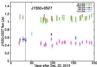
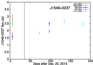
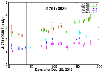
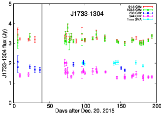
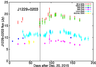
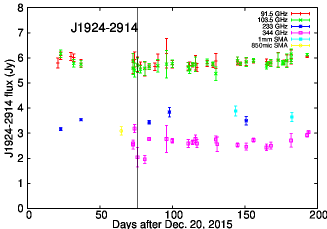
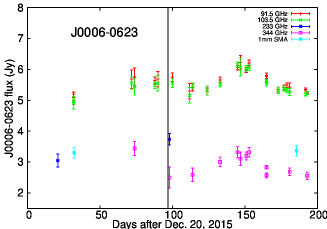
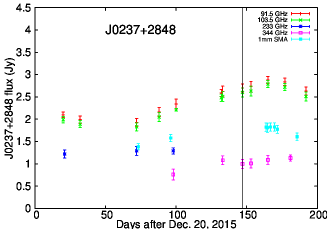
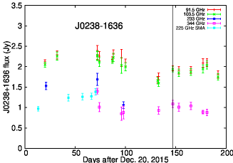
Figure 11: Flux measurements of nine quasars used as flux or secondary calibrators, over a 200 day period (Dec 20, 2015 - July 7, 2016) spanning our observations. These measurements are taken from the ALMA Calibrator Source Catalogue (https://almascience.eso.org/sc/) at 91.5, 103.5, 233 and 344 GHz or from the SMA Calibrator list (http://sma1.sma.hawaii.edu/callist/callist.html) at $\sim$225 GHz. The vertical bar corresponds to the date of our TNO observations.

A good knowledge of the 233 GHz flux of the calibrators, which may be time-varying, is critical for the reliability of the TNO flux scale. Out of the 12 quasars observed in our program, 9 are monitored from ALMA (normally at 91.5, 103.5, 233 and 344 GHz) and from the SMA at 1 mm ($\sim$225 GHz) and more occasionally at 0.85 mm ($\sim$345 GHz). These measurements are displayed in Fig. 11.1 over a 200 day period (Dec. 20, 2015 - July 7, 2016) spanning our observing period. ALMA 233 GHz measurements are the most direct source of information for our purpose, but are less abundant than at other bands. To estimate the 233 GHz fluxes at the relevant dates (marked by the vertical bars in Fig. 11.1), we combined this information with (i) $\sim$225 GHz SMA measurements and (ii) flux values in ALMA Band 3 and Band 7 and the associated spectral indices. Details follow:

• J1924-2914 (Chariklo). This object is very stable in time. Direct 233 GHz measurements from ALMA indicate a mean flux of 3.47$\pm$0.024$\pm$0.24 Jy, where the first error bar is the formal uncertainty calculated from the individual errors, and the second one is the standard deviation between the individual measurements. Spectral index (spix) fitting of the mean 91.5, 103 and 343 GHz fluxes gives spix = -0.56 and a 233 GHz flux of 3.55 Jy, fully consistent with above. Because we do not have any other quasar available to calibrate the Chariklo data, we conservatively adopt a 3.51$\pm$0.24 Jy flux, i.e. a 6.8 % uncertainty.
  

• J1733-1304 and J1751+0939 (2002 GZ₃₂). J1733-1304 is also very stable in time, with a mean flux of 1.89$\pm$0.026$\pm$0.19 Jy. Spectral index fitting of the 91.5, 103 and 343 GHz fluxes gives spix = -0.61 and a 233 GHz flux of 1.86 Jy. We initially adopt a 1.87 Jy flux. J1751+0939 is more variable, but its 233 GHz flux was measured on Jan. 26, 2016 (3 days before 2002 GZ₃₂) to be 1.35$\pm$0.09 Jy. Specifying a 1.87 Jy for the prime calibrator J1733-1304 leads to 1.28 Jy for J1751+0939 in our data. A better overall compromise is achieved by specifying 1.93 Jy for J1733-1304 (+3.2 % higher than the initial estimate, in which case the measured J1751+0939 flux is 1.31 Jy (3.3 % too low). We thus adopt 1.93$\pm$0.06 Jy (3 % uncertainty).
  

• J1550+0527 (Huya). This object shows variability and ALMA and SMA data do not appear fully consistent. For February 8, 2016, the SMA provides a 0.695$\pm$0.037 Jy flux at 225.52 GHz, i.e. 0.680$\pm$0.037 Jy at 233 GHz given a spix of -0.69$\pm$0.05, derived from 12 sets of 91, 103.5 and 343.5 GHz ALMA measurements. In contrast, ALMA provides 0.54$\pm$0.01 Jy over January 19-26, 2016. The Huya data were taken on Jan. 25. Adopting 0.68 (resp. 0.54 Jy) for J1550+0527 would yield 1.08 Jy (resp. 0.85) Jy for Titan, which was observed on the same date. Our Titan models (e.g. Moreno et al., 2012) predict 0.96 Jy for that date. We finally adopt 0.61$\pm$0.07 Jy (ie 11.4 % uncertainty) for J1550+0527. Note that J1549+0233 was observed as another phase calibrator but this object is not well enough characterized (see Fig. 11) to serve as flux calibrator.
  

• J1229+0203 (Makemake). This variable quasar, a.k.a. 3C273, is particularly monitored at the SMA, and measurements on March 2 (i.e. the same day as our Makemake observations), indicate a 225.47 GHz flux of 11.160$\pm$0.559 Jy. ALMA 91, 103.5, and 343 GHz measurements indicate a spix of -0.67$\pm$0.05, from which we derive 10.92$\pm$0.55 Jy at 233 GHz for that date. For conservativeness, and because we do not have catalog values for the second calibrator (J1303+2433), we finally adopt 10.9$\pm$0.75 Jy for J1229+0203 (6.9 % uncertainty).
  

• J0006-0623 and Pallas (Chiron). Asteroid (4) Pallas was observed as the prime calibrator for the Chiron observations. Detailed shape and thermophysical models (Müller et al., 2014) for this object (as well as for (1) Ceres, (2) Vesta and (21) Lutetia) have been demonstrated to match the ensemble of the available (and independently calibrated) Herschel PACS and SPIRE measurements over 70-500 $\mu$m within 5 %. As these models are less constrained at longer wavelengths, we prefer to use the secondary calibrator (J0006-0623) as flux calibrator, as it was remeasured at ALMA on March 27, 2016, just 1 day after the Chiron observations, with a 233-GHz flux of 3.74$\pm$0.19 Jy. On another hand, the spectral index, derived from 10 sets of ALMA 91.5, 103.5 and 343 GHz dat, is spix = -0.50$\pm$0.05. Applying this to the 343 GHz flux measured on the same date (2.5$\pm$0.34 Jy) would provide 3.03$\pm$0.41 Jy, only 1.2$\sigma$ consistent with the above. The weighted-mean average of the two values is 3.61$\pm$0.17 Jy. We still adopt the directly measured value of 3.74 Jy, but inflate somewhat the uncertainty to 0.25 Jy (6.7 %). With this, we derive a Pallas flux of 159$\pm$11 mJy for March 26, 2016, UT =14h40. The application of the above models from Müller et al. (2014) to the UT date of the Pallas measurement gives a flux of 153.7 mJy (with significant thermal lightcurve variability: 152$\pm$8 mJy), fully within the measurement error, and giving further confidence in both the flux scale and the Pallas model.
  

• J0238+1636 and J0237+2848 (Bienor). These two variable quasars have few 233 GHz measurements, but numerous 91.5, 103.5 and 343 GHz data from ALMA, including for the precise date of the Bienor data (May 15, 2016). For this date, spectral index fitting results in 233 GHz fluxes of 1.31$\pm$0.08 and 1.37$\pm$0.11 Jy respectively. We adopt a 1.29 Jy for J0238+1636 (i.e. 1.7 % less than the above flux), which using our own measurements, returns 1.40 Jy for J0237+2848 (i.e. 2.4 % more than above). Given the excellent consistency between the two quasars, we adopt a 2.5 % uncertainty on their fluxes.