Online Learning of a Memory for Learning Rates

Abstract

The promise of learning to learn for robotics rests on the hope that by extracting some information about the learning process itself we can speed up subsequent similar learning tasks. Here, we introduce a computationally efficient online meta-learning algorithm that builds and optimizes a memory model of the optimal learning rate landscape from previously observed gradient behaviors. While performing task specific optimization, this memory of learning rates predicts how to scale currently observed gradients. After applying the gradient scaling our meta-learner updates its internal memory based on the observed effect its prediction had. Our meta-learner can be combined with any gradient-based optimizer, learns on the fly and can be transferred to new optimization tasks. In our evaluations we show that our meta-learning algorithm speeds up learning of MNIST classification and a variety of learning control tasks, either in batch or online learning settings.

I Introduction

The remarkable ability of humans to quickly learn new skills stems from a hierarchical learning process. Instead of learning each new skill from scratch, a higher-level – more abstract – meta-learner acquires information about the learning process itself which is used to guide and speed up the learning of new skills. For instance, it has recently been shown that humans learn how much to correct for observed motor skill errors, and reuse such a error sensitivity memory in subsequent skill adaptation tasks [1]. In a sense, we are learning how to learn.

Most robotic learning tasks would benefit from being guided by such a meta-learner, especially when we consider the incremental learning of several skills. For example when learning to detect and recognize certain objects, it should become easier to learn how to recognize new object classes over time. The same is true for learning control tasks such as learning task-specific models of a robot’s dynamics [2]. Even single task learning settings can benefit from such a meta-learning process. For instance, consider robotic reinforcement learning tasks for which data-efficiency has been a key challenge [3, 4, 5], because acquiring new observations on a real system can be extremely costly. Meta-learning processes can help to maximize the effect of each acquired rollout.

In the machine learning community, this concept of learning-to-learn has been explored in a variety of contexts [6, 7, 8, 9] and recently received renewed attention [10, 11, 12, 13, 14].

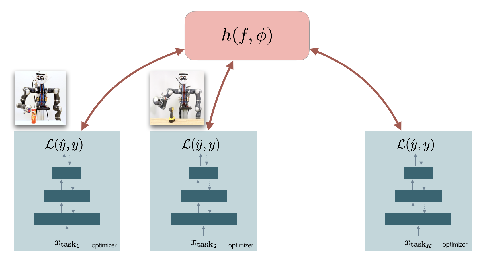
Figure 1: Sequential learning of multiple task variants (lifting pringles, lifting drill) with meta-learning. In this work, the meta-learning process learns a memory of learning rates $h$, which can be transfered between different learning problems. Transferring $h$ leads to faster learning of new task variations.

Recent work on learning how to optimize [10, 11, 12, 13, 14] employs a two-phase approach: First a meta-learner is optimized to perform well on a priori chosen tasks. Then, once this meta-learner has been trained, it is utilized in similar optimization tasks. In this work, we propose an online meta-learning algorithm, that learns to predict learning rates given currently observed gradients, while optimizing task-specific problems. We show how we can train such a memory of learning rates online and in a computationally efficient manner. Our proposed approach has several advantages: Because the meta-learning is performed online, each observed data point is utilized for both the task learning as well as the meta-learning. Not only does this mean that we utilize observed data more effectively, but also that the effect is immediate. Furthermore, online meta-learning alleviates the need for having to collect data on which to perform the learning-to-learn optimization process. Thus, our meta-learner can improve when necessary, while recent work is constrained to perform well on the task-distributions it was trained on. Finally, the resulting memory of learning rates can be transferred to similar optimization problems, to guide the learning of the new task.

Here, we evaluate our approach on two supervised learning tasks: sequential binary classification tasks on the MNIST [15] data set, and incremental learning of a robot’s inverse dynamics models. Our experiments show that when combining an optimizer with our meta-learner, we generally increase convergence speed, indicating that we utilize observed data points more effectively to reduce errors in the learning task. Furthermore, we show that when transferring our meta-learner’s internal state to new learning tasks, learning progress is faster.

In the following we start out by presenting background and related work in Section II. We then introduce our meta-learning approach in Section III. Finally we both illustrate and extensively evaluate our approach in Section IV before concluding in Section V.

II Background

As mentioned above, most learning control problems use computationally efficient variants of gradient descent

$$w^{t+1}=w^{t}-h(\nabla_{w}\mathcal{L}_{\text{task}}(f(w)))$$ (1)

where $\mathcal{L}_{\text{task}}$ typically corresponds to some loss function, $f$ the model with parameters $w$ to be optimized, and $h$ transforms the observed gradient according to some rule. Note, in the remainder of this paper we sometimes suppress the dependency of $\mathcal{L}_{\text{task}}$ on $f$, such that $\mathcal{L}_{\text{task}}(f(w))=\mathcal{L}_{\text{task}}(w)$.

In this setting meta-learning can happen at several levels. For instance, recent work [16] proposes a meta-learner that biases the learning process towards feature representations that supports few-shot learning of new tasks. On the other hand, recent learning to learn approaches [10, 11, 12, 13, 14] have been focused on learning optimizers that can be re-used for similar optimization tasks. The focus of these approaches however is on mitigating the issue of hyperparameter tuning instead of learning representations that can be transferred between (robotic) learning tasks.

Here, we present a novel meta-learning algorithm that is aligned with this second type of meta-learning, but is focused on maintaining an internal memory that can guide the learning of new tasks. In the following we review related work concerned with adaptive and learned optimizers.

II-A Adaptive First-Order Methods

In the machine learning community adaptive optimizers such as Adam [17], RMSprop [18], AdaGrad [19], AdaDelta [20] have been developed. In essence, these optimizers extend the gradient transform mapping $h$ to be a function of sufficient statistics such as the mean and variance of the observed gradients

$$w^{t+1}=w^{t}-h(\nabla_{w}\mathcal{L}_{\text{task}}(w^{t}),\mathbb{E}[\nabla\mathcal{L}_{\text{task}}(w)],\mathbb{E}[(\nabla\mathcal{L}_{\text{task}}(w))^{2}])$$ (2)

The specific gradient transform $h$ then depends on the algorithm, as has been nicely summarized in [12], Table 1. These optimizers are of linear space and time complexity with respect to the model parameters, and thus are suitable for highly parameterized models such as deep neural networks. Yet, choosing the initial learning rate for each of these methods, or which base learner to choose remains a complex manual tuning task [21, 22]. More importantly though, such adaptive methods are not meant to extract information about the learning process itself. Thus, while they have proven successful at increasing convergence speed, they are not designed to transfer knowledge to new optimization tasks.

II-B Learning to Learn

More recently, the idea of meta-learning – learning to learn – has re-gained momentum [10, 11, 12, 13, 14]. These approaches parametrize $h$ to be a function of parameters $\theta$, which determine how observed gradients are to be transformed

$$w^{t+1}=w^{t}-h(\nabla_{w}\mathcal{L}_{\text{task}}(w^{t});\theta).$$ (3)

The goal then is to learn $\theta$ to create a well-performing optimizer. In the most simple case, the parameter $\theta$ simply equals the learning rate $\eta$, which can be adapted online, as has been shown in [23]. Specifically, the authors propose to compute the gradient $\nabla_{\eta}h$ online and then perform gradient descent on the learning rate itself. While this approach is simple and general as well as computationally and memory efficient, it does not retain a state – everything is forgotten. Thus subsequent optimization tasks start from scratch.

When going from adaptive optimizers to learned optimizers we hope to have learned something that we can reuse later on; that we performed meta-learning on some level. Recent work such as [12, 10, 11] addresses this to some extent. An optimizer is trained to perform well on some pre-defined set of optimization tasks and is then used to optimize similar learning problems. While some approaches learn to transform the gradient [10, 11], others assume $h$ to be a scaling of the gradient and learn to predict the learning rates [12, 13, 14].

Our work, falls into this second category of trying to learn a coordinate-wise scaling of the gradient. To the best of our knowledge, recent work either performs learning on the step size online, but retains no memory [23], or the learning of the optimizer is performed once at the beginning and never updated again. In the latter setting, two learning phases exist: In phase one $h$ is trained, either via reinforcement learning [12, 11, 13, 14] or in a supervised manner [10]; In phase 2, the trained gradient transform $h$ is used to optimize similar learning problems.

These recent learning to learn approaches are mostly focused on mitigating the issue of hyper-parameter tuning by learning an optimizer. The goal of our approach is to learn a representation of optimal gradient transforms that can be transferred to new learning tasks. Furthermore, as opposed to previous work, we learn this representation in an online fashion while using this representation to optimize task-specific optimization problems.

III Learning a Memory for Learning Rates

In this work we investigate how we can learn a memory of learning rates online, in a computationally efficient manner. Ideally, this memory can be transferred to subsequent similar learning tasks, and speeds up convergence of that optimization problem. Furthermore, this memory should be continuously updated to be able to adapt and compress new learning rate landscapes as well.

We envision our meta-learning algorithm to be used as follows: While our systems attempts to learn a model $f(w)$ for a specific task, such as a task-specific inverse dynamics model, by minimizing the loss $\mathcal{L}_{\text{task}}(f(w))$ it also aims at building a model $h$ that can predict how much to correct for observed errors. Thus for each optimization step, we perform two updates: a gradient descent step on the task-specific model parameters, and an update our meta-learner’s memory $h$. An overview in form of a pseudo algorithm is given in 1.

In order to develop such a meta learning approach several challenges need to be met. One of the core challenges is the choice of training signal to learn such a memory on. We take inspiration from [24] and start out by showing how to derive a simple learning algorithm to train a learning rate memory $h$ for one-dimensional optimization problems. Then, we discuss a representation for $h$ that supports computationally efficient, incremental learning. Finally we show how to generalize our meta learning approach to optimization problems involving complex models such as neural networks.

III-A Training Signal for the Learning Rate Memory

Let us assume that our main objective is a learning task that requires us to minimize the objective $\mathcal{L}_{\text{task}}(w)$ with respect to parameter $w$. While optimizing parameter $w$ we also aim to learn a function $h$ that given gradient information of the main objective $\mathcal{L}_{\text{task}}(w)$, can predict a learning rate $\hat{\eta}$

$$h(z;\theta)=\hat{\eta}(z;\theta)z$$ (4)

where $\theta$ are the parameters of the learning rate memory $h$. Ideally, we would like to optimize the parameters $\theta$ with respect to the loss $\mathcal{L}_{\text{lr}}$

$$\mathcal{L}_{\text{lr}}(\eta,\hat{\eta}(z;\theta))=\frac{1}{2}(\eta-\hat{\eta}(z;\theta))^{2}$$ (5)

where $\eta$ is the true optimal learning rate, and $\hat{\eta}(z;\theta)$ the predicted learning rate for input $z=\nabla_{w}\mathcal{L}_{\text{task}}(w)$. To optimize parameters $\theta$ via gradient descent, we would need access to the true learning rate $\eta$

$$\frac{\partial\mathcal{L}_{\text{lr}}}{\partial\theta}=-(\eta-\hat{\eta}(z;\theta))\frac{\partial\hat{\eta}(z;\theta)}{\partial\theta}$$ (6)

which is unknown to us. However, by comparing the gradient of the current time step with the gradient of the previous time step, we can determine whether we over or underestimated $\eta$. If the gradient has flipped between two consecutive optimization steps, the learning rate was too large, meaning $\eta-\hat{\eta}(z;\theta)>0$. On the other hand, if the signs of the gradients are the same, then we can most likely increase the learning rate.

With this knowledge at time step $t$, the memory parameter updates can be approximated as

$$\theta^{t+1} =\theta^{t}-\xi\;(-(\eta^{t}-\hat{\eta}(z^{t};\theta^{t})))\frac{\partial\hat{\eta}(z^{t};\theta)}{\partial\theta^{t}}$$ (7)

$$\approx\theta^{t}+\xi\;\text{sign}\left(z^{t+1}z^{t}\right)\frac{\partial\hat{\eta}(z^{t};\theta^{t})}{\partial\theta}$$ (8)

where $\xi$ is a step size parameter for the gradient descent on $\theta$. The exact form of this gradient update depends on what parametric form $\hat{\eta}(z;\theta)$ takes.

Algorithm 1 Online Meta Learning

0:  initial task model $f(w^{0})$, initial meta-memory $h_{\theta^{0}}$

1:  $z^{0}=0$

2:  for  $t\in{1,...,T}$ do

3:     $z^{t}=\nabla_{w}\mathcal{L}_{\text{task}}(f(w^{t-1}))$

4:     $h_{\theta^{t}}$ = MemoryUpdate($z^{t},z^{t-1},h_{\theta^{t-1}}$) $//$ eq. 10

5:     $w^{t}=w^{t-1}-h_{\theta^{t}}(z^{t})$ $//$ eq. 4 and eq. 11

6:  end for

7:  return  $f(w^{T}),h_{\theta^{T}}$

III-B Learning Rate Memory Representation

As mentioned previously, we aim at developing an algorithm that can continuously update the learning rate memory $h$. Designing the function approximator $h$, such that forgetting of previously learned parameters is minimized, is one of the challenges of this approach. Here we choose to use locally weighted regression [25], which is known for computational efficiency and which has the capability to increase model complexity when necessary. With locally weighted regression we decompose the memory $h$ into $M$ local models $h_{m}$, each parametrized by their own parameters $\theta_{m}$.

Furthermore, in locally weighted regression, the loss function $\mathcal{L}_{lr}$ also decomposes into $M$ separately weighted losses, each dependent on only their respective parameters $\theta_{m}$:

$$\mathcal{L}_{lr}(\theta)=\sum_{m=1}^{M}\mathcal{L}_{m}(\theta)=\sum_{m=1}^{M}\psi_{m}(z)(\eta-\hat{\eta}_{m}(z,\theta_{m}))^{2}$$ (9)

where $\psi_{m}(z)$ is the weighting function that defines the active neighborhood for each local model. A standard selection of this weight function is the squared exponential kernel $\psi_{m}(z)=\exp{(-0.5\frac{(z-c_{m})^{2}}{\lambda_{m}^{2}}})$.

Using this memory representation leads to following update rule per local model

$$\theta^{t+1}_{m} =\theta^{t}_{m}+\xi\;\text{sign}\left(z^{t+1}z^{t}\right)\psi_{m}(z^{t})\frac{\partial\hat{\eta}_{m}(z^{t};\theta_{m}^{t})}{\partial\theta_{m}^{t}}.$$ (10)

Note, how only local models that are sufficiently activated require updating. Finally, at prediction time the predicted learning rate is a weighted average over all local models’ predictions:

$$\hat{\eta}=\frac{\sum_{m=1}^{M}\psi_{m}(z)\hat{\eta}_{m}(z,\theta_{m})}{\sum_{m=1}^{M}\psi_{m}(z)}$$ (11)

We now have an algorithm that can train a model $\hat{\eta}$ to predict a learning rate for one-dimensional optimization problems. An illustration of what kind of learning rate landscapes can be trained with this algorithm is given in the experimental Section in Figure 2.

As a final step, we show how this approach can be generalized to models with multiple high-dimensional parameter groups, as commonly encountered in deep learning models.

III-C Multi-Dimensional Learning Problems

Above we have assumed $z=\nabla_{w}\mathcal{L}_{\text{task}}(w)$ to be one-dimensional. A key question is how to generalize to optimization tasks that not only have high-dimensional gradients $\boldsymbol{z}=\nabla_{\boldsymbol{w}}f(\boldsymbol{w})$, but also multiple layers of parameters $\mathcal{L}_{\text{task}}(\boldsymbol{w}^{1},\dots,\boldsymbol{w}^{K})$, where $\boldsymbol{w}^{k}$ stands for the $k^{th}$ parameter group, as is typical for deep neural networks for instance.

The straightforward extension would be to compute $\text{sign}(z^{t+1}z^{t})$ as the inner product $\text{sign}({\boldsymbol{z}^{t+1}}^{T}\boldsymbol{z}^{t})$ of two consecutive gradients, and place local models in the $D_{k}$-dimensional gradient space. However, this has the following consequences: We would only learn to predict one learning rate per time step and we loose a lot of information through the inner product of the two gradients. Furthermore, the number of local models needed to cover the gradient space evenly would grow exponentially with the gradient dimension $D_{k}$ and would significantly increase memory requirements while decreasing computational efficiency.

On the other end of the spectrum we can choose $z=\nabla_{\boldsymbol{w}_{i}}\mathcal{L}_{\text{task}}(\boldsymbol{w})$ to be the partial derivative with respect to the $i^{th}$ coordinate, and create a learning rate memory per coordinate of the parameter vector $\boldsymbol{w}$. Assuming that $\boldsymbol{w}\in\mathbb{R}^{D}$, this would require $D$ memory models, each with $M$ local models. This choice, would create a learning rate prediction per gradient coordinate, and thus offers maximum flexibility. However, it also has high memory (storage) requirements.

Here we choose a different route. First, we identify natural parameter groups, such as parameters $\boldsymbol{w}^{k}$ of each hidden layer in deep neural networks. For each of these $K$ parameter groups, a memory $h^{k}$ is created. Then, for the $k^{th}$ parameter group, we pool the updates of all coordinate-wise updates, by computing the average update per local model, across all coordinates

$$a_{m,d}^{t,k} =\text{sign}\left([z]_{d,k}^{t+1}[z]_{d,k}^{t}\right)\psi^{k}_{m}([z]_{d,k}^{t})$$ (12)

$$\theta^{t+1,k}_{m} =\theta^{t,k}_{m}+\xi\;\frac{1}{D_{k}}\sum_{d}^{D_{k}}\big{(}a_{m,d}^{t,k}\;\frac{\partial\hat{\eta}^{k}_{m}([z]_{d,k}^{t};\theta^{t,k}_{m})}{\partial\theta^{k}_{m}}\big{)}.$$ (13)

where $[z]_{d,k}$ means we take the $d^{th}$ coordinate of $z=\nabla_{w^{k}}\mathcal{L}_{\text{task}}(\boldsymbol{w}^{k})$, and $D_{k}$ denotes the dimensionality of the $k^{th}$ parameter group $\boldsymbol{w}^{k}$. At prediction time, we similarly make predictions for each parameter group, per gradient coordinate $[z]_{d,k}$ to obtain a learning rate per parameter dimension.

Intuitively, this choice means that parameters within the same parameter group share the same learning rate memory, expecting that they would benefit from the same scaling behavior. With this representation our meta-learner then requires extra memory resources in the order of $O(KM)$. Furthermore, the computational complexity of the memory update as well as learning rate prediction is in the order of $O(DM)$.

III-D Implementation Details

Finally, to implement this approach, a few design choices have to be made: Each memory is pre-allocated with a fixed number $M$ of local models. Since, the localization happens in the space of one-dimensional partial gradients - we linearly space the local models centers within the range of the minimum and maximum gradient value allowed. The size of each local model is determined by parameters $\lambda_{m}$, which are chosen to create a reasonable amount of overlap between neighboring local models. Thus the more local models we allow, the smaller they become.

Furthermore, we choose local constant models, such that $\hat{\eta}(z,\theta_{m})=\theta_{m}$ in our experiments. Intuitively, this means that each $\theta_{m}$ corresponds to a learning rate value, localized in gradient space. We further use $z^{t+1}z^{t}$ and clip the resulting (absolute) value at 1 instead of the $\text{sign}(z^{t+1}z^{t})$. We have empirically found that this significantly improves the convergence since memory updates are less pronounced in regions with small gradients. Finally, at the beginning of a learning problem, when no previous memory of learning rates exist, we initialize the memories to predict an initial learning rate $\eta_{\text{init}}$, thus at the very beginning all $\theta_{m}=\eta_{\text{init}}$.

At runtime, when performing a task-specific learning problem, we then immediately start optimizing all $h^{k}$ as well. At each time step $t$, we update both, the parameters of the task-specific problem $\boldsymbol{w}$ and the learning rate memory parameters $\boldsymbol{\theta}$.

On a final note, we want to point out that our presented approach here can be used on top of any base-learner. While not explicitly noted, it is easily possible to first apply some fixed-rule based learner, such as Adam [17] to transform the gradient, and then apply our learned memory evaluation on that transformed gradient. In fact, in our experimental evaluation we include results for both basic gradient descent with learning rate memory, and Adam with learning rate memory.

IV Experiments

We evaluate our meta learning algorithm in three different settings. We start out with illustrating our approach on the Rosenbrock function, a well known non-convex optimization problem. Then we show extensive results on two learning tasks: First we investigate learning binary classifiers on the MNIST data set, both illustrating the effect of transferring the learning rate memory between similar tasks and showcasing robustness to parameter choices. Finally, we extensively evaluate our meta-learning approach on online inverse dynamics learning tasks for manipulators. We start out by explaining our experimental setup and the baseline methods we compare too.

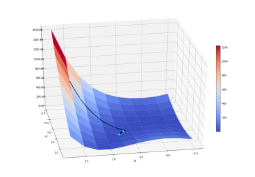
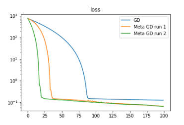
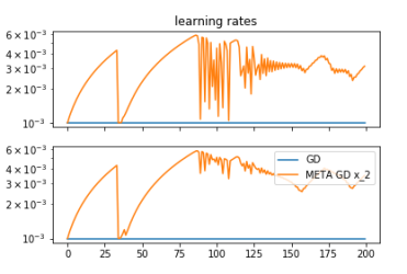
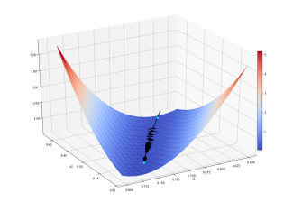
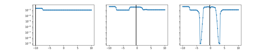
Figure 2: top row: (left) The Rosenbrock function with the meta-learners path. (middle) Convergence to minimum for gradient descent with $\eta=0.001$, and two consecutive runs of MetaGD with initial $\eta=0.001$. The first run with a learning rate memory, starts with all local models predicting the initial learning rate $\eta=0.001$, but quickly builds a model of learning rates - thus this already converges faster than without a memory. The second run of gradient descent with learning rate memory re-uses and updates the memory from run 1 and converges even faster. (right) the predicted learning rates for both dimensions, as a function of optimization steps. bottom row: (left) zoomed in Rosenbrock function to visualize path in the valley. The blue dots (in both top and bottom Rosenbrock plots) indicate where we took a snapshot of the memories. (right) 3 snapshots of the memories, with x-axis representing values of the partial derivatives $z$, and the y-axis the predicted learning rate values. The black horizontal lines, indicate the current partial gradient - at the time of the snapshot.

IV-A Baselines and Experimental Setup

As mentioned in Section III, our proposed meta-learning can be combined with different base-optimizers. We need to choose an optimizer on both hierarchies, the task specific optimizer with base learning rate $\eta$, and the meta optimizer with base learning rate $\xi$. We present results for 3 variants: basic gradient descent without meta-learning (GD), gradient descent with meta-learning with either gradient descent to update the memory (MetaGD) or with Adam [17] to update the memory (MetaGDMemAdam). For results involving neural networks, a memory of learning rates per hidden layer was learned.

We also compare to another meta-learner: L2LBGDBGD[10] is a very recent approach which treats the optimizer itself as a function approximator, typically represented by a two layer recurrent LSTM network which transform the gradients directly. L2LBGDBGD does require to learn the optimizer prior to task-specific learning. For our binary MNIST problem we sample initial neural network configurations (without structural changes) and optimize on the same data as used for evaluation. In order to avoid overfitting we run a validation epoch with a random network instance after every second optimization. After 16 rounds of optimizing a L2LBGDBGD learner we take the best L2LBGDBGD network according to the validation evaluation. All of the evaluated approaches, including our own, are based on tensorflow [26] implementations.

IV-B Rosenbrock Problem

We start off by illustrating our approach on the Rosenbrock problem, as visualized in Figure 2(left). This is a 2D optimization problem, and each dimension has it’s own memory of learning rates (as shown in Figure 2). We compare the convergence of gradient descent with $\eta=0.001$ and two consecutive runs of gradient descent with a memory of learning rates, starting from the same initial position. The memories are initialized to predict $\eta=0.001$ for the first optimization run. For the second run, we carry over the memories from the previous run.

The middle plot (top row) of Figure 2 shows the convergence of each of these optimization runs. Notice how already the first optimization run benefits from the online meta-learning. The second run converges even faster. The right plot (top row), shows the corresponding learning rates of both dimensions applied at each iteration of the second optimization run.

The bottom row shows a zoomed in Rosenbrock function, centered around the path taken by the meta-learner. The blue dots indicate where we have taken a snapshot of the learning rate memories. In the bottom right - we show the memory of the second dimension, at those 3 different time steps during the first run. We see how the memories initially learn to predict increased learning rates. Once the optimization hits the valley, it learns to predict larger learning rates as long as the optimization stays within a certain gradient range, at the borders of that gradient range the learning rate is drastically reduced to prevent jumping out of the valley.

IV-C Binary Mnist Problems

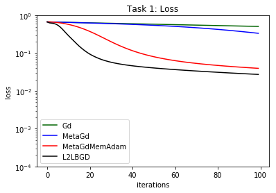
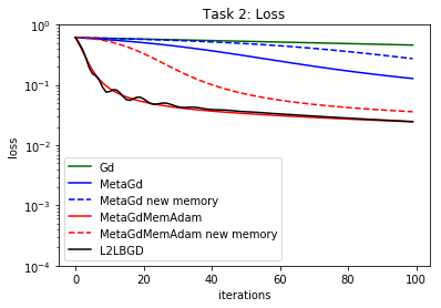
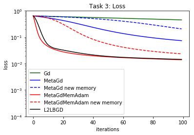
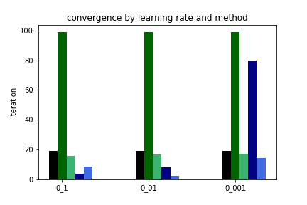
Figure 3: Results on the 3 binary MNIST learning tasks (left 3 plots top) convergence behavior of one randomly seeded (same for all optimizers) network on the 3 subsequent learning tasks with gradient descent based optimizers. (right): average number of iterations it took for the loss to drop below $0.1$ on task 1 for different initial learning rate choices ($[0.1,0.01,0.001]$). Results for meta-variants (from left to right: L2LBGDBGD, GD, MetaGD, Adam, MetaGDMemAdam) are obtained with new memories that have been initialized with the respective learning rate choice.

In our second set of experiments we look at binary MNIST classification tasks. Specifically we choose a sequence of 3 binary classification learning tasks. This experimental setup allows us to analyze the effect of transferring the memory of learning rates between similar learning problems. Task 1 learns to classify digits $1$ and $2$, task 2 digits $1$ and $3$ and task 4 digit $1$ and $4$. Note, that we simply chose the first $4$ digits for this experiment, and did not optimize that selection.

We use a neural network with the following structure: An input layer that takes the image as input; a convolutional layer followed by a max pooling operation; this is followed by a densely connected layer with dropout; finally, the output layer is another dense layer. All hidden units activation functions are rectified linear units. The loss function is the softmax cross entropy loss. For all meta-learning variants the memories (one per hidden layer) allocate a total of $M=100$ local models. Training is performed in batch-mode.

We start out by illustrating the loss convergence of optimizing the learning tasks in sequence in Figure 3 in the left three plots. In green we see basic gradient descent without any memory of learning rates. Convergence of MetaGD and MetaGDMemAdam are shown in blue and red respectively. For Task 1, no previous memory exists, thus all optimizers start with the same learning rate (except L2LBGDBGD which does not have an initial learning rate parameter). The meta variants converge faster than basic gradient descent. In task 2 we deploy each meta-variant with a new memory and with the memory trained in task 1. Meta-variants with the new memory again convergence faster then basic gradient descent; meta-variants initialized with the previously learned memory converge even faster. Notice, that we continue to update the memory of learning rates during task 2 optimization. For task 3 we see the same convergence behavior as for task 2. We also compare against L2LBGDBGD. This learned optimizer does not have a base learning rate, it requires costly training on similar network instantiations prior to usage. However, it requires a (meta) learning rate to train the optimizer. Here we chose to depict the best L2LBGDBGD optimizer we could train, which was achieved with a learning rate of $0.01$. Furthermore, the L2LBGDBGD optimizer was trained specifically for each task. Notice, on task 1 L2LBGDBGD achieves faster convergence, however any subsequent learning tasks achieve similar convergence as the MetaGDMemAdam-variant.

Note - we have achieved similar results when using Adam as the base optimizer. Adam itself, without any meta-learner, performs very well on this task, and can outperform all of the above meta-learning variants (including L2LBGDBGD). However, when combining Adam with our meta-learner, we achieve even better results. This confirms that our online meta-learning approach is versatile and can speed up convergence even when combined with an adaptive optimizer such as Adam. These results are omitted due to space limitations. Additionally, Adam does not perform well in the sequential problems such as the inverse dynamics task discussed in Sec. IV-D2.

In the right most plot of Figure 3, we depict how many iterations each optimizer variant requires to achieve an error below $0.1$, as a function of initial learning rate values. These results are averaged across 3 random seeds. Note L2LBGDBGD is constant because after having been trained no initial learning rate parameter is required. Here we include Adam, with and without meta-learning. In green we see gradient descent GD and MetaGDMemAdam, while in blue we see Adam and MetaGDMemAdam. On average, our meta-learning variants achieve a low error faster, irrespective of the initial learning rate, while gradient descent does not converge within the first 100 iterations, and Adam performs well if the learning rate is chosen high enough. This confirms that at each iteration, our meta-learning approach utilizes the observed data more efficiently and as a result leads to faster learning progress. Furthermore, our initial analysis also shows that with the use of our meta-learner the learning frameworks convergence speed is less dependent on the choice of the base learning rate. In the future, we hope to transfer this to reinforcement learning settings.

IV-D Inverse dynamics learning

In our final set of experiments we explore the use of our meta-learning variants on a typical motor control learning problem: learning of an inverse dynamics model. Learning inverse dynamics is a function approximation problem that maps the current joint position, velocities and accelerations ($q,\dot{q},\ddot{q}$) to torques ($\tau$). This is an interesting learning problem since this function mapping generally cannot be assumed to be stationary due to e.g. unknown payload changes. Hence it requires online adaptation of the learned inverse dynamics model, which can benefit from a meta-learner that is invariant to such changes. Another interesting aspect is the abundance of data, typically continuously generated at very high rates (e.g. 1 KHz). Here we consider two possibilities of processing such a high frequency data stream: we either collect task-specific data and update a task-specific inverse dynamics model in a batch setting (Sec. IV-D1); or we optimize the model online, directly on the streaming data (Sec. IV-D2).

In both experiments we use a fixed-base manipulation platform equipped with 7-DoF Kuka LWR IV arms and three-fingered Barrett Hands. We learn the inverse dynamics model for the right arm resulting in a 21-dimensional input space with one output per joint.

IV-D1 Batch Learning

For this experiment we collect data of two motion tasks (in simulation): Task 1 corresponds to acceleration policies [27] trained to move along a rectangular path in the horizontal plane, while task 2 corresponds to the same rectangular path in the vertical plane. These movements are performed under strong perturbations of the assumed inverse dynamics model. Data collection consists of recording joint position, velocities, accelerations and torques at each time step (1ms). Each task is trained on $10000$ collected data points. Per task, we train a neural network per joint in a single batch setting, meaning that the full dataset is used for each optimization step. The neural network structure has 3 densely connected hidden layers with $[100,50,10]$ hidden units, respectively. All activation functions are rectified linear units, and dropout prior to the output layer. The loss function is the mean squared error (MSE) on the predicted torque values.

We perform the two learning tasks in sequence: first we train a dynamics model on task 1, then we learn a new (uninitialized) dynamics model for task 2. The convergence of each optimization task is shown in Figure 4. Notice how using and optimizing our meta-learner while optimizing the inverse dynamics model for task 1 already leads to faster convergence. When transferring the meta-learner for task 2 learning convergence to a low error is even faster. Thus, improving the convergence by re-using the meta-optimizer while adapting to new tasks allows to perform faster incremental learning of task specific inverse dynamics models.

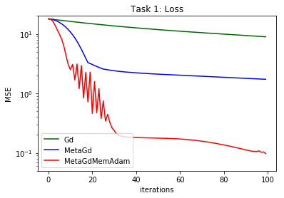
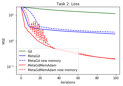
Figure 4: Learning task-specific inverse dynamics models in batch mode, on the 1st joint of our 7-DOF manipulator. Meta-Learning helps to convergence faster within task 1 already, when transferring the learned memory of learning rates to task optimization, convergence speed is increased.

IV-D2 Sequential Online Learning

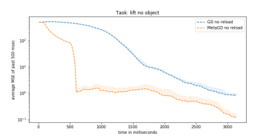
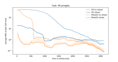
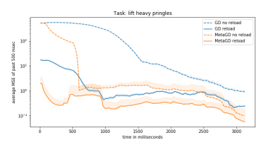
Figure 5: Loss convergence when online learning a inverse dynamics model on the 1st joint of our 7-DOF manipulator. (left) uninitialized network is updated online with GDand MetaGDwith an uninitialized memory. (middle) online learning convergence on task-variant 2 with and without reloading the network and meta-learner from task-variant 1. (right) convergence on task-variant 3 with and without reloading.

In this experiment we consider the task of lifting an object with different configurations (no, light, heavy object) on the real manipulation platform. We collect position, velocities, accelerations and torques at each time step (1ms), resulting in three data sets with more then 3000 samples each. Further, we execute each task variation 10 times to assess the variance of the learning process. All results presented are averaged across these 10 trials.

In this experiment we have 3 learning phases, first we train an uninitialized network and meta-learner on the lifting no object task. Then this network is further trained on the data corresponding to task-variant 2: light object. Finally, the same network is re-used and further adapted on task-variant 3: heavy lifting. This scenario tests, how quickly we can adapt previously trained networks, with and without the meta-learner.

Again, we train one network per joint. The neural network structure consists of 3 densely connected hidden layers with $[100,50,10]$ hidden units, respectively. All activation functions are rectified linear units. The loss function used to optimize the parameters is the mean-squared-error (MSE). For all experiments we use $M=200$ local models for each memory (per layer), a memory learning rate of $0.005$, and gradient clipping of $1.0$. These values have been determined empirically. We present results for joint 1 since it exhibits large torque variations given payload changes. Notice, the initial high loss values are due to the torque range which is between 30 and 35 N/m hence the model optimized with mean squared error loss has to first adjust for this offset. Different to the previous experiment each learning phase is updating the network online using sequential data batches of size 10, meaning we take data samples collected within the last 10 milliseconds and perform one optimization step. Every data sample is processed exactly once. This is a very challenging setting since gradients are highly correlated and the overall optimization step should be faster than 10 ms. From our empirical evaluation we found that Adam does not perform well in these very correlated settings which is why we omit the results. Computation times for both MetaGD and basic GD are less then 3 ms on standard hardware, hence, fast enough to consume a continuous data stream of inverse dynamics data.

In Figure 5 we illustrate the convergence of the loss as we are moving along the trajectory of each lifting task, when using $\eta=0.0001$. In the left most plot, we see convergence on task 1 of GD and MetaGD. The middle plot shows convergence on task 2 (light object), comparing learning from scratch (no reloading of network or meta-learner) with continual learning of the previously learned network (reload), for both basic GD and MetaGD. As we can see, when warm-starting, we immediately start out with a lower error for both GD and MetaGD. With MetaGD we reduce the experienced error faster. Note, even without reloading, GD and MetaGD (net and memory uninitialized) manage to learn a good model by the end of the movement, however they produce larger prediction errors at the beginning of the movement. Similar behavior can be observed on the final task of lifting the heavy object.

We performed this experiment for $\eta=[0.01,0.001,0.0001]$ and summarize the mean loss for the first 500 ms of the task execution of joint 1 in Table I. We are mostly interested in assessing fast convergence, therefore the focus on the beginning of the task. The data clearly illustrates the benefit of using our proposed MetaGD, that reaches a low loss faster, meaning using less data, in almost all settings. Interesting to note is that with a really high learning rate all methods achieve very good results e.g. $0.01$ heavy, yet, due to the high learning rate there is a high chance that some gradient in the sequence will drive the model into a “bad” parameter space, resulting in poor convergence ($0.01$ no object).

$\eta$		GD	MetaGD	GD	MetaGD
	lift	noreload	noreload	reload	reload
	no object	180.062	228.421	180.062	228.421
$0.01$	light	234.276	228.704	55.407	18.926
	heavy	220.249	167.623	0.034	0.027
	no object	119.317	65.221	119.317	65.221
$0.001$	light	110.396	63.952	2.233	0.692
	heavy	113.62	66.958	0.618	0.454
	no object	468.849	80.219	468.849	80.219
$0.0001$	light	489.441	78.799	10.712	0.593
	heavy	513.898	82.804	6.444	0.694
	no object	256.076	124.62	256.076	124.62
average	light	278.038	123.818	22.784	6.737
	heavy	282.589	105.795	2.365	0.392

TABLE I: MSE of the first $500$ ms of each task execution.

V Discussion and Future Work

We have presented a novel meta-learning algorithm, that can incrementally learn a memory of learning rates as a function of current gradient observations. We have discussed how to learn this memory in a computationally efficient manner and have shown that deploying such a meta-learner leads to consistently faster convergence in the number of iterations. Furthermore, we have shown that memories of learning rates can be transferred between similar learning tasks, and speed up convergence of the new – previously unseen – learning problems.

However, thus far this effect has been constrained to base optimizers that do not transform the gradient before updating the learning rate memory. Thus, in future work we aim to investigate whether we can extend the state with which the memory is indexed beyond simple gradient information. The hope would be that this would allow the memory to capture even more complex learning rate landscapes. It further could enable to maintain the underlying structure between tasks, better coping with forgetting of learning rate memories. The challenge here is to do so while maintaining computational efficiency.

Another interesting avenue would be to use meta-learning for transfer learning. This is especially interesting in robotics since real robot experiments are very costly and in general do not scale in comparison to simulation. Yet, simulation results typically do not translate directly to the real world. Thus, the meta-learner will hopefully result in less real robot experiments required to achieve good performance since it can optimize the problem faster, thus, transferring information from simulation to real world experiments. Finally, we have shown how a simple update rule as discussed in Section III can create a very effective meta-learner. Yet, it would be interesting to combine our incremental meta-learner with even more expressive objectives that can guide the learning of the memory.

References

- [1] D. J. Herzfeld, P. A. Vaswani, M. K. Marko, and R. Shadmehr, “A memory of errors in sensorimotor learning.” Science, 2014.
- [2] D. Kappler, F. Meier, N. Ratliff, and S. Schaal, “A new data source for inverse dynamics learning,” in Proc. of the IEEE/RSJ Conference on Intelligent Robots and Systems, 2017.
- [3] M. Deisenroth and C. E. Rasmussen, “Pilco: A model-based and data-efficient approach to policy search,” in Proc. of the International Conference on machine learning (ICML), 2011, pp. 465–472.
- [4] S. Gu, T. Lillicrap, Z. Ghahramani, R. E. Turner, B. Schölkopf, and S. Levine, “Interpolated Policy Gradient: Merging On-Policy and Off-Policy Gradient Estimation for Deep Reinforcement Learning,” ArXiv e-prints, Jun. 2017.
- [5] S. Kamthe and M. P. Deisenroth, “Data-Efficient Reinforcement Learning with Probabilistic Model Predictive Control,” ArXiv e-prints, Jun. 2017.
- [6] S. Hochreiter, A. S. Younger, and P. R. Conwell, “Learning to learn using gradient descent,” in Proc. Intl. Conf. On Arti. Neural Networks, 2001.
- [7] J. Schmidhuber, “Evolutionary principles in self-referential learning,” On learning how to learn: The meta-meta-… hook.) Diploma thesis, Institut f. Informatik, Tech. Univ. Munich, 1987.
- [8] N. Schweighofer and K. Doya, “Meta-learning in reinforcement learning,” Neural Networks, vol. 16, no. 1, pp. 5–9, 2003.
- [9] R. Vilalta and Y. Drissi, “A perspective view and survey of meta-learning,” Artificial Intelligence Review, vol. 18, no. 2, 2002.
- [10] M. Andrychowicz, M. Denil, S. Gomez, M. W. Hoffman, D. Pfau, T. Schaul, and N. de Freitas, “Learning to learn by gradient descent by gradient descent,” in Advances In Neural Information Processing Systems, 2016, pp. 3981–3989.
- [11] K. Li and J. Malik, “Learning to optimize,” arXiv preprint arXiv:1606.01885, 2016.
- [12] C. Daniel, J. Taylor, and S. Nowozin, “Learning step size controllers for robust neural network training.” in AAAI, 2016, pp. 1519–1525.
- [13] S. Hansen, “Using deep q-learning to control optimization hyperparameters,” arXiv preprint arXiv:1602.04062, 2016.
- [14] J. Fu, Z. Lin, M. Liu, N. Leonard, J. Feng, and T.-S. Chua, “Deep q-networks for accelerating the training of deep neural networks,” arXiv preprint arXiv:1606.01467, 2016.
- [15] Y. LeCun, “The mnist database of handwritten digits.” 1998.
- [16] C. Finn, P. Abbeel, and S. Levine, “Model-agnostic meta-learning for fast adaptation of deep networks,” arXiv e-prints:1703.03400, 2017.
- [17] D. P. Kingma and J. Ba, “Adam: A Method for Stochastic Optimization,” ArXiv e-prints, Dec. 2014.
- [18] T. Tieleman and G. Hinton, “Lecture 6.5-rmsprop: Divide the gradient by a running average of its recent magnitude.” COURSERA: Neural Networks for Machine Learning, 4 2012.
- [19] J. Duchi, E. Hazan, and Y. Singer, “Adaptive subgradient methods for online learning and stochastic optimization,” Journal of Machine Learning Research, vol. 12, no. Jul, pp. 2121–2159, 2011.
- [20] M. D. Zeiler, “ADADELTA: An Adaptive Learning Rate Method,” ArXiv e-prints, Dec. 2012.
- [21] I. Loshchilov and F. Hutter, “SGDR: Stochastic Gradient Descent with Warm Restarts,” ArXiv e-prints, Aug. 2016.
- [22] P. Goyal, P. Dollár, R. Girshick, P. Noordhuis, L. Wesolowski, A. Kyrola, A. Tulloch, Y. Jia, and K. He, “Accurate, Large Minibatch SGD: Training ImageNet in 1 Hour,” ArXiv e-prints, Jun. 2017.
- [23] A. Gunes Baydin, R. Cornish, D. Martinez Rubio, M. Schmidt, and F. Wood, “Online Learning Rate Adaptation with Hypergradient Descent,” ArXiv e-prints, Mar. 2017.
- [24] M. Riedmiller and H. Braun, “A direct adaptive method for faster backpropagation learning: the RPROP algorithm,” in IEEE International Conference on Neural Networks, 1993.
- [25] S. Schaal and C. G. Atkeson, “Constructive incremental learning from only local information,” Neural computation, vol. 10, no. 8, 1998.
- [26] M. Abadi, A. Agarwal, P. Barham, E. Brevdo, Z. Chen, C. Citro, G. S. Corrado, A. Davis, J. Dean, M. Devin et al., “Tensorflow: Large-scale machine learning on heterogeneous distributed systems,” arXiv e-prints:1603.04467, 2016.
- [27] A. J. Ijspeert, J. Nakanishi, H. Hoffmann, P. Pastor, and S. Schaal, “Dynamical movement primitives: learning attractor models for motor behaviors,” Neural computation, vol. 25, no. 2, pp. 328–373, 2013.