Einstein-Podolsky-Rosen steering: Its geometric quantification and witness

Abstract

We propose a measure of quantum steerability, namely a convex steering monotone, based on the trace distance between a given assemblage and its corresponding closest assemblage admitting a local-hidden-state (LHS) model. We provide methods to estimate such a quantity, via lower and upper bounds, based on semidefinite programming. One of these upper bounds has a clear geometrical interpretation as a linear function of rescaled Euclidean distances in the Bloch sphere between the normalized quantum states of: (i) a given assemblage and (ii) an LHS assemblage. For a qubit-qubit quantum state, these ideas also allow us to visualize various steerability properties of the state in the Bloch sphere via the so-called LHS surface. In particular, some steerability properties can be obtained by comparing such an LHS surface with a corresponding quantum steering ellipsoid. Thus, we propose a witness of steerability corresponding to the difference of the volumes enclosed by these two surfaces. This witness (which reveals the steerability of a quantum state) enables one to find an optimal measurement basis, which can then be used to determine the proposed steering monotone (which describes the steerability of an assemblage) optimized over all mutually-unbiased bases.

I Introduction

Quantum entanglement Einstein et al. (1935), Einstein-Podolsky-Rosen (EPR) steering Schrödinger (1935), and Bell nonlocality Bell (1964) are different forms of quantum nonlocality Wiseman et al. (2007). These quantum correlations are powerful resources for quantum engineering, quantum cryptography, quantum communication, and quantum information processing Horodecki et al. (2009); Brunner et al. (2014); Gallego and Aolita (2015). Taking an operational perspective Wiseman et al. (2007), EPR steering can certify the entanglement between two systems when one of the measurements is untrusted, i.e., no assumptions are made on the functioning of the measurement device. On the other hand, Bell nonlocality can certify the entanglement with the untrusted measurements on both sides. One can also certify an entangled state by performing quantum state tomography with all-trusted measurement devices. Thus, EPR steering is a form of quantum correlation, which can be classified between entanglement and Bell nonlocality, in the following meaning: it certifies the entanglement between two systems assuming trusted measurements only on one of these Wiseman et al. (2007). Eighty years of research on EPR steering has resulted in many experimental demonstrations Ou et al. (1992); Hald et al. (1999); Bowen et al. (2003); Howell et al. (2004); Saunders et al. (2010); Wittmann et al. (2012); Bennet et al. (2012); Händchen et al. (2012); Smith et al. (2012); Steinlechner et al. (2013); Schneeloch et al. (2013); Su et al. (2013); Sun et al. (2016); Cavalcanti et al. (2009) and various applications Reid (1989); Pusey (2013); Walborn et al. (2011); Kogias et al. (2015); Costa and Angelo (2016), which include multipartite quantum steering He and Reid (2013); Li et al. (2015a); Xiang et al. (2017); Milne et al. (2014); Cheng et al. (2016), the correspondence with measurement incompatibility Cavalcanti and Skrzypczyk (2016); Uola et al. (2014); Quintino et al. (2014); Chen et al. (2016a); Uola et al. (2015), one-way steering Sun et al. (2016); Wollmann et al. (2016); Skrzypczyk et al. (2014); Cavalcanti and Skrzypczyk (2017), one sided device-independent processing in quantum key distribution Branciard et al. (2012), continuous-variable EPR steering Tatham et al. (2012); He et al. (2015); Wang et al. (2015); Xiang et al. (2017), as well as temporal Chen et al. (2014, 2016b); Bartkiewicz et al. (2016, 2016); Ku et al. (2016); Li et al. (2015b) and spatio-temporal steering Chen et al. (2017).

In recent years, several measures of steering, such as steerable weight Skrzypczyk et al. (2014), steering robustness Piani and Watrous (2015), steering fraction Hsieh et al. (2016), steering cost Das et al. (2017), intrinsic steerability Kaur et al. (2017), as well as the relative entropy of steering Gallego and Aolita (2015); Kaur and Wilde (2017) have been proposed (see also the review Cavalcanti and Skrzypczyk (2017)). All these quantifiers are monotones under one-way local operations assisted by classical communication (one-way LOCCs) Gallego and Aolita (2015). More recently, several works using the geometrical approaches to steering have been considered, such as depicting quantum correlations for two-qubit states Jevtic et al. (2014, 2015) and a geometrical approach to witness steering Nguyen and Vu (2016a, b). Here, we would like to use the consistent steering robustness (CSR) introduced by Cavalcanti et al. Cavalcanti and Skrzypczyk (2016) and the quantum steering ellipsoid (QSE) introduced by Jevtic et al. Jevtic et al. (2014, 2015) to construct such a geometric witness. The QSE provides a visualization and geometric representation of any two-qubit state McCloskey et al. (2017); Cheng et al. (2016); Bowles et al. (2016); Milne et al. (2014). Specifically, the QSE for a given two-qubit state corresponds to the set of all Bloch vectors of one qubit (say Bob), which can be prepared by another qubit (say Alice) by considering all possible projective measurements on her qubit Jevtic et al. (2014, 2015).

In this work, we propose a distance between assemblages based on the trace distance between single elements. Given an assemblage, a trace-distance measure of steerability is then proposed as the distance to the closest unsteerable assemblage. Here, we prove that the consistent trace-distance measure of steerability is a convex steering monotone, with respect to restricted one-way LOCCs introduced in Ref. Kaur et al. (2017). We note that our proposal is reminiscent of other distance-based measures of various quantum phenomena. These include “nonclassical distance” for quantifying the quantumness of optical fields Hillery (1987); Miranowicz et al. (2015), distance-based measures of entanglement Vedral et al. (1997), trace-distance measures of coherence Rana et al. (2016), or trace-distance measures quantifying Bell nonlocality Brito et al. (2017).

In order to estimate the proposed steering monotone, we provide lower and upper bounds that can be efficiently computed by semidefinite programs (SDPs) Vandenberghe and Boyd (1996). Specifically, a lower bound is obtained via an operator-norm distance, whereas a few upper bounds are found by applying various known steering measures Cavalcanti and Skrzypczyk (2016); Skrzypczyk et al. (2014); Piani and Watrous (2015); Bavaresco et al. (2017).

Moreover, we introduce the local-hidden-state (LHS) surface as a way of visualizing steerability properties of a two-qubit quantum state in the Bloch sphere. In particular, these notions connect to the QSE and provide a witness of steerability based on the different volumes enclosed by the two surfaces. This steerability witness enables finding an optimal measurement basis McCloskey et al. (2017). Thus, this is particularly important for calculating the proposed steering monotone optimized over all mutually-unbiased bases. To illustrate the usefulness of LHS surfaces, we provide the explicit solution of the LHS surface for the Werner states. Moreover, we present a few upper and lower bounds of the steerability measure for the Werner, Horodecki, and rank-2 Bell-diagonal states Werner (1989); Miranowicz et al. (2008). Note that this approach, despite some resemblance, essentially differs from, e.g., the relative entropy of entanglement Vedral et al. (1997); Vedral and Plenio (1998); Miranowicz et al. (2008) and the nonclassical distance Hillery (1987); Miranowicz et al. (2015) used for quantifying the quantumness of bosonic systems.

This paper is organized as follows. In Sec.II we summarize the basic notions concerning EPR steering. In Sec. III we introduce a steering quantifier; we also prove that it is a monotone under restricted one-way LOCCs, and provide computable lower and upper bounds for it. In Sec. IV we introduce a steering witness based on the notion of LHS surface and discuss its properties. In Sec. V we apply our results to several interesting examples. Finally, in Sec. VI, we provide the conclusions and outlook for our work.

II Preliminary notions

EPR steering can be operationally defined as the success of the following task Wiseman et al. (2007): One party, say Alice, tries to convince another party, say Bob, that they share an entangled state $\rho_{AB}$. To accomplish this task, Bob asks Alice to perform some measurements, described by positive-operator valued measures (POVMs) $A_{a|x}$ with $A_{a|x}\geq 0$, satisfying $\sum_{a}A_{a|x}=\openone$, where $x$ denotes the basis of the measurement, $a$ is its outcome, and $\openone$ is an unit operator. Bob’s measurements are assumed to be fully characterized by quantum mechanics. Therefore, he can perform quantum state tomography and obtain the unnormalized quantum states $\sigma_{a|x}=\text{tr}_{A}(\rho_{AB}A_{a|x}\otimes\openone)$. In particular, any $\{A_{a|x}\}_{a,x}$ gives rise to a collection of unnormalized quantum states $\{\sigma_{a|x}\}_{a,x}$, which are termed as an assemblage. An assemblage also includes the information of Alice’s marginal statistics $p(a|x)=\text{tr}(\sigma_{a|x})$.

The assemblage $\{\sigma_{a|x}\}_{a,x}$ is unsteerable if it admits an LHS model:

$$\sigma_{a|x}=\sigma_{a|x}^{\text{US}}=\sum_{\lambda}p(\lambda)p(a|x,\lambda)\sigma_{\lambda}~{}\quad\forall a,x.$$ (1)

An LHS model can be understood as follows: Alice sends a preexisting quantum state $\sigma_{\lambda}$ according to her input $x$ and outcome $a$ with a probability distribution $p(\lambda)$ and a conditional probability distribution $p(a|x,\lambda)$. In this sense, the assemblage, received by Bob, is just a classical postprocessing of the set of states $\{\sigma_{\lambda}\}_{\lambda}$, which is clearly independent of Alice’s measurements. Likewise, a quantum state $\rho_{AB}$ is called steerable if the given assemblage does not admit an LHS model. Such a state is necessarily entangled, but the converse is not true Wiseman et al. (2007).

In the context of a resource theory of steering Gallego and Aolita (2015), the most general free operation for EPR steering is a stochastic one-way LOCC, defined as follows. Given an assemblage $\{\sigma_{a|x}\}_{a,x}$, Bob performs a quantum measurement on his system. The measurement is described by a completely positive trace-nonincreasing map $\varepsilon$ defined by

$$\begin{split}\varepsilon(\sigma_{B}):=\sum_{\omega}K_{\omega}(\sigma_{B})K^{\dagger}_{\omega},~{}~{}~{}\text{such~{}~{}~{}~{}that}~{}~{}\sum_{\omega}K^{\dagger}_{\omega}K_{\omega}\leq\openone,\end{split}$$ (2)

for the reduced state $\sigma_{B}$ of Bob, where $K_{\omega}$ is the Kraus operator associated with a classical outcome $\omega$. In the most general case, the set of classical outcomes is a coarse graining of the set of possible $\omega$ (quantum instruments may be defined by more than one Kraus operator), but, as we discuss below, there is no loss of generality by considering that each outcome $\omega$ is associated with a single Kraus operator $K_{\omega}$.

After such an operation, Bob communicates with Alice obtaining a classical result $\omega$ prior to her measurement. She applies a local deterministic wiring map $W_{\omega}$, defined explicitly below, described by the normalized conditional probability distributions: $p(x|x^{\prime},\omega)$, describing the generation of any initial input $x$ from final input $x^{\prime}$ and Bob’s result $\omega$, and $p(a^{\prime}|a,x,x^{\prime},\omega)$, describing the generation of Alice’s final outcome $a^{\prime}$ from $a$, $x$, $x^{\prime}$, and $\omega$. The final assemblage with input $x^{\prime}$ and outcomes $\omega,a^{\prime}$ becomes

$$\{\sigma_{a^{\prime}|x^{\prime}}^{\omega}\}_{a^{\prime},x^{\prime}}:=M_{\omega}(\{\sigma_{a|x}\}_{a,x}).$$ (3)

Here, $M_{\omega}(\{\sigma_{a|x}\}_{a,x}):=K_{\omega}W_{\omega}(\{\sigma_{a|x}\}_{a,x})K_{\omega}^{\dagger}$ is a subchannel of the map $M:=\sum_{\omega}M_{\omega}$ when Bob post-selects the $\omega$th outcome with probability $p(\omega)$=Tr[$M_{\omega}(\sum_{a}\{\sigma_{a|x}\}_{a,x})$], while

$$W_{\omega}(\{\sigma_{a|x}\}_{a,x})=\{\sum_{a,x}p(x|x^{\prime},\omega)p(a^{\prime}|a,x,x^{\prime},\omega)\sigma_{a|x}\}_{a^{\prime},x^{\prime}}$$ (4)

is a deterministic wiring map. We recall that a function $S$ is a steering monotone (see Ref. Gallego and Aolita (2015)) if it is zero for unsteerable assemblages and it is a monotone, i.e., it does not increase (on average), under one-way LOCCs, i.e.,

$$\sum_{\omega}p(\omega)S\left(\frac{M_{\omega}(\{\sigma_{a|x}\}_{a,x})}{p(\omega)}\right)\leq S(\{\sigma_{a|x}\}_{a,x}),$$ (5)

for a given assemblage $\{\sigma_{a|x}\}_{a,x}$. Note that the particular case when $\sum_{\omega}p(\omega)=1$ or $\sum_{\omega}K^{\dagger}_{\omega}K_{\omega}=\openone$, is called a deterministic one-way LOCC. Otherwise, this is a stochastic one-way LOCC. Finally, we note that the use of a coarse-grained set of classical outcomes, simply implies the equality of some of Alice wirings, i.e., $W_{\omega}=W_{\omega}^{\prime}$, if $\omega$ and $\omega^{\prime}$ are coarse-grained into the same classical outcome.

In the following, we consider a restricted set of one-way LOCC, which has been proposed in Ref. Kaur et al. (2017). This restriction consists of requiring that Alice’s choice of wiring does not depend on the classical outcome $\omega$ obtained by Bob via local operations. This restriction can be motivated by practical reasons Kaur et al. (2017): Given a spatial separation between Alice and Bob, the protocol may be more efficient if Alice directly applies her operation on her system instead of waiting for communication with Bob. This “restriction hypothesis” translates into the condition $p(x|x^{\prime},\omega)=p(x|x^{\prime})$, and hence into the condition

$$W_{\omega}(\{\sigma_{a|x}\}_{a,x})=\{\sum_{a,x}p(x|x^{\prime})p(a^{\prime}|a,x,x^{\prime},\omega)\sigma_{a|x}\}_{a^{\prime},x^{\prime}}.$$

III Geometric quantifiers of steerability

III.1 Trace-distance steerability measure

The (quantum) trace distance is a metric to distinguish two density operators $\rho$ and $\rho^{\prime}$, i.e., $D_{Q}(\rho,\rho^{\prime}):=\frac{1}{2}\|\rho-\rho^{\prime}\|$, where $\|X\|:=\operatorname{tr}[|X|]$ is the trace norm. When $\rho$ and $\rho^{\prime}$ commute, the trace distance reduces to the classical trace distance, i.e., the Kolmogorov distance Fuchs and van de Graaf (1999), which can be defined as $D_{C}(P,P^{\prime}):=\frac{1}{2}\sum_{x}|P(x)-P^{\prime}(x)|$ for two probability distributions $P$ and $P^{\prime}$.

One can easily prove the properties of a metric, i.e., it is (i) non-negative, (ii) symmetric, (iii) vanishes if and only if $\rho=\rho^{\prime}$, and (iv) satisfies the triangle inequality. Similarly, we can define the distance between two assemblages as

$$D_{A}(\{\sigma_{a|x}\}_{a,x},\{\sigma_{a|x}^{\prime}\}_{a,x})=\sum_{a,x}p(x)D(\sigma_{a|x},\sigma_{a|x}^{\prime}),$$ (6)

where $D(a,b):=\frac{1}{2}\|a-b\|$, and $\{\sigma_{a|x}\}_{a,x}$ and $\{\sigma_{a|x}^{\prime}\}_{a,x}$ are two assemblages with the same number of inputs $N_{x}$. In general, $p(x)$ can be chosen to be uniform with respect to the number of measurement settings, i.e., $\frac{1}{N_{x}}$. As for $D_{Q}$, one can easily prove that $D_{A}$ satisfies all the properties of a metric (cf. Appendix A). Note that trace-distance between two assemblages is first introduced by Kaur et al. Kaur and Wilde (2017). Nevertheless, our definition is different from theirs.

In the following, we want to introduce a measure of steerability based on the distance of a given assemblage from the set of unsteerable states. Several convex steering monotones have been introduced, with different properties and different interpretations. Our goal here is to introduce a different measure based on the trace-distance between assemblages. We introduce a quantifier, called consistent trace-distance measure of steerability, defined as the minimal trace distance to the “consistent” unsteerable assemblage Cavalcanti and Skrzypczyk (2016), namely,

$$\begin{split}S_{\rm TD}(\{\sigma_{a|x}\}_{a,x}):=\min\Big{\{}D_{A}({\{\sigma_{a|x}\}_{a,x},\{\rho_{a|x}\}_{a,x}})\Big{|}\\ {\{\rho_{a|x}\}_{a,x}\in\text{LHS}},\ \sum_{a}\rho_{a|x}=\sum_{a}\sigma_{a|x},\ \forall x\ \Big{\}}.\end{split}$$ (7)

where ${\rm LHS}$ denotes the set of unsteerable assemblages, i.e., those admitting an LHS model given by Eq. (1). In Appendix B, we prove that $S_{\rm TD}$ is a restricted convex steering monotone.

Unfortunately, it is quite hard to calculate such a monotone without knowing the structure of LHSs. Instead, we find a way to derive lower and upper bounds based on SDPs.

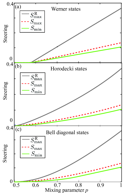
Figure 1: Upper ($S_{\rm max}^{\text{R}}$ and $S_{\rm max}$) and lower ($S_{\rm min}$) bounds of the steerability measure $S_{\rm TD}$ for (a) the Werner states (rank-4 Bell-diagonal states), (b) Horodecki states, and (c) rank-2 Bell-diagonal states vs their mixing parameter $p$. A given assemblage is created when Alice performs three mutually-unbiased measurements (eigenvectors of the Pauli spin matrices $X,~{}Y$, and $Z$). Here, we compute the unsteerable assemblage obtained from the restricted-noise consistent steering robustness (RNCSR, $S_{\rm CSR}^{\text{R}}$) bounded by $S_{\rm max}^{\text{R}}$, and the consistent steering robustness (CSR, $S_{\rm CSR}$) bounded by $S_{\rm max}$. As can be seen, the steerability monotonically increases with increasing parameter, for (b), (c) $p\geq 1/2$ and (a) $p\geq 1/\sqrt{3}$. Note that the meaning of the mixing parameter $p$ is completely different in (a), (b), and (c) as given by the definitions of the corresponding states in Sec. V.A, V.B, and V.C.

III.2 Upper bound based on the restricted-noise consistent steering robustness

An upper bound of $S_{\rm TD}$ can be obtained via the notion of steering robustness Piani and Watrous (2015), i.e., the amount of noise that can be added to an assemblage to make it unsteerable, and the notion of CSR Cavalcanti and Skrzypczyk (2016), i.e., with the requirement that the noise assemblage has the same reduced state. We introduce a robustness measure based on this kind of mixing with a reduced state, which can be summarized as follows: Given an assemblage $\{\sigma_{a|x}\}_{a,x}$ and the associated reduced state $\sigma_{B}=\sum_{a}\sigma_{a|x}$, we define a steering monotone as

$$\begin{split}S_{\rm CSR}^{\text{R}}(\{\sigma_{a|x}\}_{a,x})=\min\Big{\{}t\left|\ \frac{\sigma_{a|x}+t[p(a|x)\sigma_{B}]}{1+t}\right.\\ \text{ is unsteerable }\Big{\}},\end{split}$$ (8)

which can be referred to as a restricted-noise consistent steering robustness (RNCSR), where $p(a|x)=\operatorname{tr}(\sigma_{a|x})$. The quantity $S_{\rm CSR}^{\text{R}}$ can be efficiently computed as an SDP (see Appendix C).

Given an assemblage $\{\sigma_{a|x}\}_{a,x}$, the unsteerable assemblage, which is obtained as the solution of the SDP for calculating ${\rm S}_{\rm CSR}^{\text{R}}$, is denoted by $\{\sigma^{\text{R}}_{a|x}\}_{a,x}$ . We can then easily compute the distance between these two assemblages as follows

$$\begin{split}D_{A}(\{\sigma_{a|x}\}_{a,x},\{\sigma^{\text{R}}_{a|x}\}_{a,x})&=\\ \frac{1}{N_{x}}\frac{t_{\text{min}}}{1+t_{\text{min}}}&\sum_{a,x}p(a|x)D(\tilde{\sigma}_{a|x},\sigma_{B}),\end{split}$$ (9)

where $t_{\text{min}}$ is the optimal parameter $t$ obtained from Eq. (8) and the tilde denotes normalized states, e.g., $\tilde{\sigma}_{a|x}=\sigma_{a|x}/\operatorname{tr}(\sigma_{a|x})$. As a consequence, the minimal trace distance between an assemblage and the restricted set of unsteerable assemblage obtained via mixing with noise $\sigma_{B}$, corresponds to substituting $t_{\text{min}}$ into the solution of an SDP for the $S_{\rm CSR}^{\text{R}}$ in Eq. (9). Thus, an upper bound on $S_{\rm TD}$ can be simply given by

$$S_{\max}^{\text{R}}(\{\sigma_{a|x}\}_{a,x})=D_{A}(\{\sigma_{a|x}\}_{a,x},\{\sigma^{\text{R}}_{a|x}\}_{a,x}).$$ (10)

Note that if Bob’s system is a qubit, then $S^{\text{R}}_{\max}(\{\sigma_{a|x}\}_{a,x})$ corresponds to a half of the sum of all the Euclidean distances between the Bloch vectors $\tilde{\sigma}_{a|x}$ and $\sigma_{B}$ in the Bloch sphere multiplied by the probability distribution $p(a|x)$ and the scaling factor $t_{\min}/[N_{x}(1+t_{\min})]$. Mathematically, this can be expressed as

$$S^{\rm{R}}_{\rm{max}}(\{\sigma_{a|x}\}_{a,x})=\sum_{a,x}\frac{p(a|x)\,t_{\min}}{N_{x}(1+t_{\min})}\frac{|\vec{p}_{a|x}-\vec{q_{b}}|}{2},$$ (11)

where $|\vec{a}-\vec{b}|$ denotes the Euclidean distance between vectors $\vec{a}$ and $\vec{b}$. Moreover, $\vec{p}_{a|x,i}=\text{tr}(\tilde{\sigma}_{a|x}\sigma_{i})$ and $\vec{q}_{b,i}=\text{tr}(\sigma_{B}\sigma_{i})$ (for $i=1,2,3$) are the components of the Bloch vectors of $\tilde{\sigma}_{a|x}$ and $\sigma_{B}$, respectively, and $\{\sigma_{1},\sigma_{2},\sigma_{3}\}\equiv\{X,Y,Z\}$ denote the Pauli operators.

III.3 Upper bound based on the consistent steering robustness

Here we provide another upper bound on the steering monotone $S_{\rm TD}$, which is also based on the CSR. We show that this new bound is even tighter than that of $S_{\rm max}^{\text{R}}(\{\sigma_{a|x}\}_{a,x})$, as defined in Eq. (10).

The CSR is defined as follows Cavalcanti and Skrzypczyk (2016):

$$\begin{split}S_{\rm CSR}(\{\sigma_{a|x}\}_{a,x})=\min\Big{\{}t\left|\ \frac{\sigma_{a|x}+t\tau_{a|x}}{1+t}\right.\\ \text{ is unsteerable, and }\sum_{a}\tau_{a|x}=\sigma_{B},\ \forall x\Big{\}},\end{split}$$ (12)

where $\{\tau_{a|x}\}_{a,x}$ is an arbitrary noise assemblage with the same reduced state.

Similarly to $S_{\rm max}^{\text{R}}$, an upper bound of $S_{\rm TD}$ can be obtained from the optimal solution $\{\sigma^{\text{CSR}}_{a|x}\}_{a,x}$ of an SDP for the CSR. Note that although the $\{\sigma^{\text{CSR}}_{a|x}\}_{a,x}$ is an optimal unsteerable assemblage, it may not be closest according to the trace distance. Thus, an upper bound based on the CSR can be defined as

$$\begin{split}S_{\rm max}(\{\sigma_{a|x}\}_{a,x})=D_{A}(\{\sigma_{a|x}\}_{a,x},\{\sigma^{\text{CSR}}_{a|x}\}_{a,x}).\end{split}$$ (13)

Because $S_{\rm max}^{\text{R}}$ was obtained for a restricted noise, so it is obvious that the following inequality holds in general:

$$S_{\rm max}\leq S_{\rm max}^{\text{R}}.$$ (14)

III.4 Lower bound based on operator norm

In this section, we show how to compute a lower bound of $S_{\rm TD}$ as an SDP. Without loss of generality, we can write the assemblage $\{\rho_{a|x}\}_{a,x}\in\text{LHS}$, as $\rho_{a|x}=\sum_{\lambda}\delta_{a,\lambda_{x}}\sigma_{\lambda}$, where $\lambda$ is a vector $(\lambda_{x})_{x}$ and $\delta_{a,\lambda_{x}}$ represent the deterministic strategy for choosing the assemblage element $\sigma_{\lambda}$ Pusey (2013). For consistency, we assume the condition $\sum_{\lambda}\sigma_{\lambda}=\sum_{a}\rho_{a|x}=\sigma_{B}$. Then we note that the trace norm can be lower bounded by the operator norm

$$\|A\|_{\infty}:=\min\{\mu|-\mu\openone\leq A\leq\mu\openone\},$$ (15)

i.e., $\|A\|_{\infty}\leq\|A\|$ for all operators $A$. Combining the lower bound based on this norm with the definition of the unsteerable assemblage, we obtain the following lower bound for $S_{\rm TD}(\{\sigma_{a|x}\}_{a,x})$:

$$\begin{split}S_{\rm min}:=\min_{\begin{subarray}{c}\sigma_{\lambda}\end{subarray}}:&\frac{1}{2N_{x}}\sum_{a,x}\|\sigma_{a|x}-\sum_{\lambda}\delta_{a,\lambda_{x}}\sigma_{\lambda}\|_{\infty}\\ \text{subject to: }&\sum_{\lambda}\sigma_{\lambda}=\sigma_{B};\\ &\sigma_{\lambda}\geq 0,\quad\forall\lambda;\end{split}$$ (16)

where $\delta_{a,\lambda_{x}}$ is the usual deterministic strategy for the LHS model. Now, we can rewrite the above problem as the following SDP:

$$\begin{split}S_{\rm min}=\min_{\begin{subarray}{c}\mu_{a,x},\sigma_{\lambda}\end{subarray}}:&\frac{1}{2N_{x}}\sum_{a,x}\mu_{a,x}\\ \text{subject to: }&-\mu_{a,x}\openone\leq\sigma_{a|x}-\sum_{\lambda}\delta_{a,\lambda_{x}}\sigma_{\lambda}\leq\mu_{a,x}\openone\ \\ &\sum_{\lambda}\sigma_{\lambda}=\sigma_{B};\\ &\sigma_{\lambda}\geq 0,\quad\forall\lambda.\end{split}$$ (17)

By definition, we have $0\leq\mu_{a,x}\leq 1$, so the same holds for the solution of the SDP. This implies that the primal SDP problem is bounded. Moreover, it is also strictly feasible, e.g., just take any strictly positive assemblage $\sigma_{\lambda}$, consistent with the reduced state $\sigma_{B}$, and $\mu_{a,x}=1$ for all $a,x$. This implies the strong duality condition, i.e., the primal and dual SDPs have the same optimal value.

Note, however, that the operator norm quantifier $S_{\rm min}(\{\sigma_{a|x}\}_{a,x})$ is not a convex steering monotone, since the operator-norm distance is, in general, not contractive under completely positive trace-nonincreasing maps.

Finally, we have the following lower and upper bounds:

$$\begin{split}S_{\rm min}(\{\sigma_{a|x}\}_{a,x})\leq S_{\rm TD}(\{\sigma_{a|x}\}_{a,x})\leq S_{\rm max}(\{\sigma_{a|x}\}_{a,x})\\ \leq S_{\rm max}^{\text{R}}(\{\sigma_{a|x}\}_{a,x}),\end{split}$$ (18)

which can be efficiently computed via our SDPs. A clear comparison of these three upper bounds and lower bound for some states is shown in Fig. 1.

IV Geometric witness of steerability

In Sec. III, we concentrated on assemblages, but in this section we focus on steerability of a quantum state rather than assemblages.

In addition to the geometrical picture introduced in Sec. III, we provide a way to visualize two-qubit steering properties through the notion of a LHS surface and a QSE. We first recall that the QSE Jevtic et al. (2014) is defined as the surface of normalized assemblages $\tilde{\sigma}_{a|x}=\sigma_{a|x}/\text{tr}(\sigma_{a|x})$, obtained by Bob for all possible projective measurements of Alice. All projective measurements on Alice’s side form the surface of the QSE, while the POVMs correspond to the points in the interior. The QSE centers at $\tilde{c}=(\tilde{b}-T^{\text{T}}\tilde{a})/(1-\tilde{a}^{2})$ with the orientation and semiaxes lengths $s_{i}=\sqrt{q_{i}}$ given by the eigenvectors and eigenvalues $q_{i}$ of the ellipsoid matrix

$$Q=\frac{1}{1-\tilde{a}^{2}}(T^{\text{T}}-\tilde{b}\tilde{a}^{\text{T}})\left(\openone+\frac{\tilde{a}\tilde{a}^{\text{T}}}{1-\tilde{a}^{2}}\right)(T-\tilde{a}\tilde{b}^{\text{T}}),$$ (19)

where $\tilde{a}$ and $\tilde{b}$ are the Bloch vectors of the reduced states of Alice and Bob, respectively. Here, $T$ is the correlation matrix with elements $T_{jk}=\text{tr}[\rho_{\text{AB}}\sigma_{j}\otimes\sigma_{k}]$ (for $j,k=1,2,3$), where $\rho_{\text{AB}}$ is the bipartite state shared by Alice and Bob.

We can analogously define the corresponding LHS surface. Instead of considering all possible single measurements, however, we need to fix a measurement assemblage for Alice. In this case, we assume that Alice can perform three mutually unbiased measurements  on her side with outcomes $\pm 1$. Consequently, Bob obtains the assemblage $\{\sigma_{a|x}\}_{a,x}$, consisting of six terms. To compute the closest unsteerable assemblage, $\{\sigma_{a|x}^{\text{US}}\}_{a,x}$, we restrict to the RNCSR case which can be computed as an SDP. By normalizing such an assemblage, $\tilde{\sigma}_{a|x}^{\text{US}}=\sigma_{a|x}^{\text{US}}/\text{tr}(\sigma_{a|x}^{\text{US}})$, Bob obtains six vectors in the Bloch sphere. The LHS surface is then obtained when Alice performs all possible rotations of her mutually-unbiased measurement bases.

Intuitively, the bipartite state $\rho_{AB}$ is unsteerable if its LHS surface and QSE are identical because $\{\tilde{\sigma}_{a|x}\}_{a,x}=\{\tilde{\sigma}_{a|x}^{\text{US}}\}_{a,x}$. Moreover, it is clear that ${\rm conv}($LHS surface$)$ is always contained in ${\rm conv}($QSE$)$, where we denoted with ${\rm conv}$ the convex hull of the points in the corresponding surface. In fact, given $\{\sigma_{a|x}\}_{a,x}$, the corresponding solution $\{\sigma_{a|x}^{\text{US}}\}_{a,x}$, computed via an SDP for the RNCSR, satisfies $\operatorname{tr}(\sigma_{a|x})=\operatorname{tr}(\sigma_{a|x}^{\text{US}})$, and hence $\tilde{\sigma}_{a|x}^{\text{US}}$ is a convex hull of points inside the QSE, namely,

$$\tilde{\sigma}_{a|x}^{\text{US}}=\frac{\tilde{\sigma}_{a|x}+t\sigma_{B}}{1+t}.$$ (20)

Therefore, we can geometrically witness steering when

$$\Delta V\equiv V_{\text{QSE}}-V_{\text{LHS surface}}>0,$$ (21)

where $V_{\text{QSE}}$ and $V_{\text{LHS surface}}$ are the volumes of the QSE and LHS surface, respectively.

Note that the steering witness $\Delta V$ focuses on the steerability of a quantum state, while the proposed steering monotone $S_{\rm TD}$ describes the steerability of an assemblage. Thus, one could think that it is rather hard, in general, to compare these approaches and to show which of these is more useful. Now we would like to explain now an important relation between the witness $\Delta V$ and the steering monotone $S_{\rm TD}$. Note that $S_{\rm TD}$ is defined on an assemblage, hence, it requires the measurement settings to be fixed. In contrast to this, the calculation of $\Delta V$ involves looking at all possible mutually-unbiased bases; hence, it provides a more complete information about the steerability of a given state. In addition, McCloskey et al. McCloskey et al. (2017) showed that the geometric information encoded in the QSE often provides the optimal measurement directions, corresponding to the three ellipsoid semi-axes. Similarly, the LHS surface provides the information about the measurement directions giving usually the highest steering monotone $S_{\rm TD}$.

The concept of the LHS surface can be generalized to include different SDP characterizations of the “closest” unsteerable assemblages, e.g., via the steering robustness Piani and Watrous (2015) or other quantifiers Cavalcanti and Skrzypczyk (2017). Moreover, such a notion can also be generalized beyond the qubit case. The interest for the present approach is motivated by the possibility of visualizing the steering properties of a state onto the Bloch sphere and its relations with the QSE.

V Applications

In Sec. III, we provided examples of lower and upper bounds for our steering monotone $S_{\rm TD}$. In what follows, we demonstrate the usefulness of the LHS surface and the trace-distance measures of steerability in several related examples.

We analyze three important prototype classes of states (i.e., the Werner, Horodecki, and Bell-diagonal states), which are formed by the singlet state $|S\rangle$ mixed with three different states. Thus, the meaning of the mixing parameter is different in these states although denoted, for simplicity, by the same symbol $p$. Specifically, (a) for the Werner states, the singlet state $|S\rangle$ is mixed with a (separable) completely mixed state, which is not orthogonal to $|S\rangle$; (b) for the Horodecki states, $|S\rangle$ is mixed with a separable state, which is orthogonal to $|S\rangle$; and (c) for the Bell-diagonal states, $|S\rangle$ is mixed with another maximally entangled state (i.e., the entangled triplet state), which is orthogonal to $|S\rangle$.

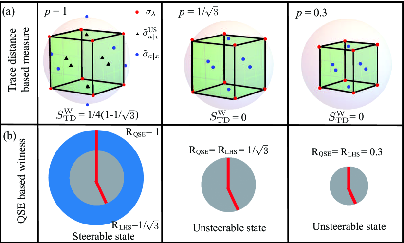
Figure 2: EPR steerability of the Werner states: (a) steerability measure $S_{\rm TD}^{\rm W}$, which is based on trace distance, and (b) steerability witness given, by Eq. (21), which is based on the volume of the QSE and LHS surface. For (a), we use the three Pauli bases to obtain the preexisted states $\{\sigma_{\lambda}\}_{\lambda}$ (red circles), steered states $\{\tilde{\sigma}_{a|x}\}_{a,x}$ (black triangles), and the unsteerable assemblage $\{\tilde{\sigma}_{a|x}^{\text{US}}\}_{a,x}$ (blue circles), respectively. The auxiliary green cube helps one to see the relative positions of the LHS and the steered states. As expected, when $p\geq$ $1/\sqrt{3}$, we find that the positions of the steered states are outside the LHSs. On the other hand, the Bloch vectors of $\{\tilde{\sigma}_{a|x}^{\text{US}}\}_{a,x}$ remain as ($\pm 1/\sqrt{3}$,0,0), (0,$\pm 1/\sqrt{3}$,0) and (0,0,$\pm 1/\sqrt{3}$), independent of $p$. This is because the maximal length of a Bloch vector is equal to unity. When $p\leq 1/\sqrt{3}$, the unsteerable states $\{\tilde{\sigma}_{a|x}^{\text{US}}\}_{a,x}$ are exactly identical to the steered states $\{\tilde{\sigma}_{a|x}\}_{a,x}$. For (b), we show the QSE and LHS surface for different values of $p$. Both surfaces are spheres, so it is sufficient to show the two-dimensional projection. The outer and inner circles are the QSE and LHS surface, respectively. These circles are centered at $\tilde{c}=(0,0,0)$. The three semiaxes of the QSE lie along $x$, $y$, and $z$. However, the orientations of the three LHS axes are the same as those of the QSE, but the length is $p$ only when $0<p<1/\sqrt{3}$. When $p>1/\sqrt{3}$, the lengths are fixed at $1/\sqrt{3}$. In other words, the QSE and LHS surfaces are identical when $p\leq 1/\sqrt{3}$. Once $p\geq 1/\sqrt{3}$, the LHS surface is fixed, but the QSE expands with $p$.

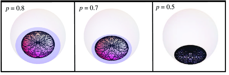
Figure 3: QSE-based witness of the steerability of the Horodecki states. As can be seen, a given state is steerable if the LHS surface and QSE are not identical. Horodecki states are unsteerable if the parameter $p=1/2$. Otherwise these states are steerable. Note that one of the lower bounds of $S_{\rm{TD}}$ corresponds to the distance between the inner and outer surfaces (i.e., the Euclidean distance between $\tilde{\sigma}_{a|x}^{\text{US}}$ and $\tilde{\sigma}_{a|x}$ in the Bloch sphere) multiplied by the probability distribution $p(a|x)$ and some scaling factor defined in the text.

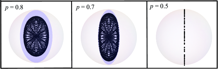
Figure 4: QSE-based witness of the steerability of the rank-2 Bell-diagonal states. As can be seen, a given state is steerable if its LHS surface and QSE are not identical. The Bell-diagonal states are unsteerable if the parameter $p=1/2$. Otherwise these are steerable.

V.1 Steerability of Werner states

We analytically show the solution of the LHS surface for the Werner states Werner (1989), which are mixtures of the singlet state and the maximally-mixed state, i.e.,

$${\rho^{\rm W}(p)=p|S\rangle\langle S|+(1-p)\frac{\openone}{4}},$$ (22)

where ${|S\rangle=1/\sqrt{2}(|10\rangle-|01\rangle)}$ and $0\leq p\leq 1$ is the mixing weight. It is clear that the Werner states are rank-4 Bell-diagonal states for $p<1$. When Alice applies the three Pauli operators ($X$, $Y$, and $Z$) to measure a given Werner state, the corresponding Bloch vectors of Bob’s normalized assemblage are ($\pm p$,0,0), (0,$\pm p$,0), and (0,0,$\pm p$). The simplest solution of the preexisted quantum states $\{\sigma_{\lambda}\}_{\lambda}$ is located at ($\pm p$,$\pm p$,$\pm p$) in the Bloch sphere. On the other hand, the LHSs are the mixtures of four preexisted states according to the strategy $p(\lambda)$ with probability $p(a|x,\lambda)=1/4$. When $p\leq 1/\sqrt{3}$, the LHSs $\tilde{\sigma}_{a|x}^{\text{US}}$ are identical to the steered states $\tilde{\sigma}_{a|x}$. As $p\geq$ $1/\sqrt{3}$, the Bloch vectors of $\tilde{\sigma}_{a|x}^{\text{US}}$ are fixed at ($\pm 1/\sqrt{3}$,0,0), (0,$\pm 1/\sqrt{3}$,0), and (0,0,$\pm 1/\sqrt{3}$) as shown in Fig. 2. This is because the maximal length of a Bloch vector is equal to unity. The optimal value of $p$ for the LHS and preexisted states is $1/\sqrt{3}$, coinciding with the upper bound $S_{\max}^{\text{R}}$ on the steering inequality $\langle XX\rangle+\langle YY\rangle+\langle ZZ\rangle\leq\sqrt{3}$ Cavalcanti et al. (2009). However, the set of steered states $\tilde{\sigma}_{a|x}$, i.e., the QSE, gradually expands with $p$. One can also rotate the measurement settings on Alice’s side, but keep them mutually unbiased. Once all sets of the three measurements are performed, Bob obtains the LHS surface, which is the set of all $\tilde{\sigma}_{a|x}^{\text{US}}$ (see Fig. 2). One can solve analytically this simple case and show that the LHS surface of the Werner state is actually a sphere, centered at $\tilde{c}=(0,0,0)$ as the QSE, with radius $1/\sqrt{3}$ for $p\geq 1/\sqrt{3}$, and radius $p$ otherwise (see Fig. 2 and Appendix D). The trace distance between them is equal to

$$D_{A}^{\rm W}(\{\sigma_{a|x}\}_{a,x})=\frac{1}{4}\left(p-\frac{1}{\sqrt{3}}\right)$$ (23)

for $p\geq 1/\sqrt{3}$, and $0$ otherwise, which is identical to quarter the Euclidean distance between the $\tilde{\sigma}_{a|x}^{\text{ US}}$ and $\tilde{\sigma}_{a|x}$. Interestingly, the $D_{A}^{\rm W}(\{\sigma_{a|x}\}_{a,x})$, which can be computed by our analytical solution for the Werner states, is smaller than $S_{\text{max}}$ and the same as $S_{\text{min}}$. Thus, we conclude that $S^{\rm{W}}_{\text{TD}}$=$D_{A}^{\rm W}(\{\sigma_{a|x}\}_{a,x})$, where the superscript $W$ indicates that the results are for the Werner states. Note that in this example, we considered only three Pauli measurement bases. It can be constructive to compare Fig. 2 for the Werner states with Figs. 3 and 4 for other special states.

Another comparison of various upper and lower bounds for the Werner states is shown in Fig. 1(a). It is seen that the upper bounds of $S_{\rm TD}^{\rm{W}}$ for the Werner states are vanishing for the mixing parameter $p\leq 1/\sqrt{3}$ and are linearly increasing with $p>1/\sqrt{3}$. This is contrary to the behavior of the same bounds for the states analyzed in Figs. 1(b) and 1(c).

V.2 Steerability of Horodecki states

The Horodecki states are the mixtures of a maximally entangled state, say the singlet state $|S\rangle$, and a separable state, say $|00\rangle$, i.e.,

$$\rho^{\rm H}(p)=p|S\rangle\langle S|+(1-p)|00\rangle\langle 00|.$$ (24)

In Fig. 3, we show that the LHS surfaces, which are computed by the RNCSR for the Horodecki states, are similar to those for the Werner states. When $0\leq p\leq 1/2$, the LHS surface and QSE are identical. Therefore, the trace distance between a given assemblage and unsteerable assemblage, which we consider $X,~{}Y,$ and $Z$, is $0$, when $0\leq p\leq 1/2$. As $p\geq 1/2$, the QSE and LHS surfaces gradually expand but the QSE expands more rapidly than the LHS surface. The trace distance of the assemblages also increases when $1/2\leq p\leq 1$ [see Figs. 1(b)]. Via numerical fitting of the computed points, we find that the LHS surface associated with the Horodecki states is consistent with the corresponding QSE. Another comparison of various upper and lower bounds for the Horodecki states is shown in Fig. 1(b).

V.3 Steerability of rank-2 Bell-diagonal states

In general, Bell-diagonal states of two qubits are mixtures of the four maximally-entangled quantum states. Here, for simplicity, we consider special rank-2 Bell-diagonal states, i.e., mixtures of the singlet state $|S\rangle$ and a triplet state $|T\rangle=1/\sqrt{2}(|10\rangle+|01\rangle)$, i.e.,

$$\rho^{\rm B}(p)=p|S\rangle\langle S|+(1-p)|T\rangle\langle T|,$$ (25)

where $p$ is the mixing weight. In Fig. 4, we show that the LHS surface, which was computed by the RNCSR, is identical to the QSE only when $p=1/2$; otherwise, these are different. The distance between a given assemblage and unsteerable assemblage, which we consider $X,~{}Y,$ and $Z$, also reveals the same behavior, as shown in Fig. 1(c). However, the LHS surface of these Bell-diagonal states cannot be fitted by an ellipsoid.

The upper bounds of $S_{\rm TD}$ for the Horodecki states [as shown in Fig. 1(b)] and the Bell-diagonal states [Fig. 1(c)] are vanishing for the mixing parameter $p\in[0,1/2]$ and $p=1/2$, respectively. Moreover, these bounds are nonlinearly increasing with $p\geq 1/2$. This is in contrast to those upper bounds for the Werner states [shown in Fig. 1(a)], which vanish for $p\in[0,1/\sqrt{3}]$ and are linearly increasing with $p>1/\sqrt{3}$. As already mentioned in the introduction to Sec. V, the meaning of the mixing parameter $p$ for these three classes of states is completely different. By analyzing the Werner states, we see that, by mixing the singlet state $|S\rangle$ with the maximally mixed state $\openone/4$, the steerability of such “noisy” singlet states is completely destroyed for a wider range of the values of the mixing parameter $p$ in comparison to the other two cases, i.e., to the mixing of the singlet state $|S\rangle$ with a state $|\psi\rangle$ orthogonal to $|S\rangle$ both for the separable state $|\psi\rangle=|00\rangle$ (which results in the Horodecki states) and for the maximally entangled state $|\psi\rangle=|T\rangle$ (which results in the Bell-diagonal states).

VI Conclusions and outlook

In this work, we defined the trace-distance between two assemblages and the corresponding measure of steerability based on this distance. We have shown that this measure of steerability is indeed a convex steering monotone under restricted one-way LOCCs. We provided a way of estimating such a quantity via lower and upper bounds based on SDPs. Specifically, a lower bound is based on the operator norm, while a few upper bounds are found by applying various steering measures, including the CSR Cavalcanti and Skrzypczyk (2016), and a restricted version of the CSR. Using the latter bound, we proposed a way of visualizing the steerability property of a quantum state in the Bloch sphere via the notion of a LHS surface, which relates the steerability problem, in the sense of the existence of a LHS model, with the notion of QSEs.

We computed EPR steerability by describing a set of states in the Bloch sphere. We did not construct a space of assemblages. Thus, we defined, in particular, the upper bound $S_{\max}^{\text{R}}$, which can be directly computed by summing up (with some coefficients) all the “Euclidean distances” between Bloch vectors. Therefore, $S_{\max}^{\text{R}}$ has a clear geometrical meaning. Moreover, in Sec. V.A, we also pointed out that $S_{\rm TD}$ for the Werner states (as denoted by $S_{\rm TD}^{\rm W}$) has a direct relation to the distance between the set of states in the Bloch sphere. The monotone $S_{\rm TD}^{\rm W}$ is a linear function of the distance from the points $(x,0,0)$, $(0,x,0)$, and $(0,0,x)$ (where $x=\pm 1/\sqrt{3}$ ) of the Bloch sphere to a normalized quantum state of its assemblage in the Bloch sphere, when the mixing parameter $p>1/\sqrt{3}$. Thus, by referring to a “geometrical” interpretation, we mean the Euclidean distance between quantum states in the Bloch sphere.

We defined the witness $\Delta V$ of steerability corresponding to the difference of the volumes enclosed by the QSE and the LHS surface. The LHS surfaces enable calculation of the proposed steering monotone $S_{\rm TD}$ optimized over all mutually-unbiased bases. We remark that this observation relates the different concepts of (i) the steering witness $\Delta V$, which reveals the steerability of a quantum state, and (ii) the steering monotone $S_{\rm TD}$, which describes the steerability of an assemblage.

Our study stimulates some further investigations. First, it is known that the QSE has an analytical representation. Therefore, it is natural to ask if the LHS surface also has an analytical formulation, at least, for some specific states. Our analysis shows that this is the case for the Werner states and we have numerical evidence that the same could be possible for the Horodecki states. Second, since we have obtained the witness of steerability for a given quantum state, given in Eq. (21), it is interesting to investigate whether such a difference of volumes, i.e., between the QSE and LHS surface, has some physical meaning and can be used to obtain a new steering monotone for a quantum state.

Appendix A Metric properties

Here we define the trace distance between two assemblages as

$$D_{A}(\{\sigma_{a|x}\}_{a,x},\{\rho_{a|x}\}_{a,x})=\frac{1}{N_{x}}\sum_{a,x}D(\sigma_{a|x},\rho_{a|x}),$$ (26)

where $D(\rho,\rho^{\prime}):=\frac{1}{2}\|\rho-\rho^{\prime}\|$ and $\|X\|:=\text{tr}[|X|]$ is the trace norm.

Now we show that $D_{A}$ satisfies the following three basic properties required for a true metric: (1) It is obvious that $D_{A}(\{{\sigma_{a|x}}\}_{a,x},\{{\rho_{a|x}}\}_{a,x})=0$ because $\{\sigma_{a,x}\}_{a|x}$ and $\{\rho_{a|x}\}_{a,x}$ are the same.

(2) Here, we prove that the trace distance between two assemblages is symmetric:

$$D_{A}(\{{\sigma_{a|x}}\}_{a,x},\{{\rho_{a|x}}\}_{a,x}) =\frac{1}{N_{x}}\sum_{a,x}D(\{\sigma_{a|x}\}_{a,x},\{\rho_{a|x}\}_{a,x})$$ (27)

$$=\frac{1}{N_{x}}\sum_{a,x}D(\{\rho_{a|x}\}_{a,x},\{\sigma_{a|x}\}_{a,x})$$

$$=D_{A}(\{{\rho_{a|x}}\}_{a,x},\{{\sigma_{a|x}}\}_{a,x}).$$

The second equality is based on a property of the matrix norm.

(3) We now show that the trace distance between two assemblages satisfies the triangle inequality,

$$D_{A}(\{{\sigma_{a|x}}\}_{a,x},\{{\rho_{a|x}}\}_{a,x})=\frac{1}{N_{x}}\sum_{a,x}D(\{\sigma_{a|x}\}_{a,x},\{\rho_{a|x}\}_{a,x})$$ (28)

$$\leq\frac{1}{N_{x}}\sum_{a,x}\left[D(\{\sigma_{a|x}\}_{a,x},\{\theta_{a|x}\}_{a,x})+D(\{\theta_{a|x}\}_{a,x},\{\rho_{a|x}\}_{a,x})\right]$$

$$=D_{A}(\{{\sigma_{a|x}}\}_{a,x},\{{\theta_{a|x}}\}_{a,x})+D_{A}(\{{\theta_{a|x}}\}_{a,x},\{{\rho_{a|x}}\}_{a,x}).$$

The first inequality follows from the property of the trace norm. This completes our proof.

Appendix B Restricted convex steering monotone

First, we recall the definition of a convex steering monotone introduced in Ref. Gallego and Aolita (2015) with the restrictive assumption from Ref. Kaur et al. (2017), namely, the independence of Alice’s choice from Bob’s outcome $\omega$.

A function $S$, relating assemblages with non-negative real numbers, is a convex steering monotone if it satisfies the following:

• It vanishes for unsteerable assemblages:

  $$S(\{\sigma_{a|x}\}_{a,x})=0\quad\text{for~{}all}\quad\{\sigma_{a|x}\}_{a,x}\in\text{LHS}.$$ (29)

• (Monotonicity) $S$ is non-increasing, on average, under restricted one-way LOCCs, i.e.,

  $$\sum_{\omega}P(\omega)\ S\left(\left\{\frac{\sigma_{a^{\prime}|x^{\prime}}^{\omega}}{P(\omega)}\right\}_{a^{\prime},x^{\prime}}\right)\leq S(\{\sigma_{a|x}\}_{a,x}),$$ (30)

  where

  $$\sigma^{\omega}_{a^{\prime}|x^{\prime}}:=\sum_{a,x}p(x|x^{\prime})p(a^{\prime}|a,x,x^{\prime},\omega)K_{\omega}\sigma_{a|x}K_{\omega}^{\dagger}$$ (31)

  is an assemblage obtained from the initial assemblage $\{\sigma_{a|x}\}_{a,x}$ by performing restricted one-way LOCCs. Here, $K_{\omega}$ is a Kraus operator with outcome $\omega$ and $\sum_{i}K_{i}^{\dagger}K_{i}=\openone$, while $p(x|x^{\prime})$ and $p(a^{\prime}|a,x,x^{\prime},\omega)$ are classical postprocessing, i.e., deterministic wiring maps, on Alice’s side.

• (Convexity) Given a real number $0\leq\mu\leq 1$, and two assemblages $\{\sigma_{a|x}\}_{a,x}$ and $\{\sigma^{\prime}_{a|x}\}_{a,x}$, the steering function $S$ satisfies the inequality

  $$\begin{split}S(\mu\{\sigma_{a|x}\}_{a,x}+(1-\mu)\{\sigma^{\prime}_{a|x}\}_{a,x})\hskip 56.9055pt\\ \leq\mu S(\{\sigma_{a|x}\}_{a,x})+(1-\mu)S(\{\sigma^{\prime}_{a|x}\}_{a,x}).\end{split}$$

Given an assemblage, we recall that the consistent trace-distance measure of steerability is defined as

$$\begin{split}S_{\rm TD}(\{\sigma_{a|x}\}_{a,x}):=\min\Big{\{}D_{A}({\{\sigma_{a|x}\}_{a,x},\{\rho_{a|x}\}_{a,x}})\Big{|}\\ {\{\rho_{a|x}\}_{a,x}\in\text{LHS}},\ \sum_{a}\rho_{a|x}=\sum_{a}\sigma_{a|x},\ \forall x\ \Big{\}}.\end{split}$$ (32)

where $D_{A}(\{\sigma_{a|x}\}_{a,x},\{\sigma_{a|x}^{\prime}\}_{a,x})=\sum_{a,x}p(x)D(\sigma_{a|x},\sigma_{a|x}^{\prime})$. First, it is obvious that the trace-distance measure of steerability satisfies condition (i). Before we prove that the trace-distance measure of steerability satisfies condition (ii), we prove the following Lemma.

Lemma 1

. Let $\{\mathcal{I}_{\omega}\}_{\omega}$ be a collection of positive trace non-increasing maps, summing up to a trace non-increasing map $\mathcal{I}:=\sum_{\omega}\mathcal{I}_{\omega}$. Then, for any Hermitian operators $T$ and $S$, we have

$$\sum_{\omega}\operatorname{tr}[|\mathcal{I}_{\omega}(T)-\mathcal{I}_{\omega}(S)|]\leq\operatorname{tr}[|T-S|].$$ (33)

Proof.— The proof is a slight modification of the one by Ruskai Ruskai (1994). Let us define $X:=T-S$. Since $X$ is Hermitian, by spectral decomposition, we can write $X=X^{+}-X^{-}$, with $X^{+},X^{-}\geq 0$. We then have

$$\begin{split}\sum_{\omega}\operatorname{tr}[|\mathcal{I}_{\omega}(T)-\mathcal{I}_{\omega}(S)|]=\sum_{\omega}\operatorname{tr}[|\mathcal{I}_{\omega}(X)|]\\ =\sum_{\omega}\operatorname{tr}[|\mathcal{I}_{\omega}(X^{+})-\mathcal{I}_{\omega}(X^{-})|]\\ \leq\sum_{\omega}\operatorname{tr}[|\mathcal{I}_{\omega}(X^{+})|]+\operatorname{tr}[|\mathcal{I}_{\omega}(X^{-})|]\\ =\sum_{\omega}\operatorname{tr}[\mathcal{I}_{\omega}(X^{+})]+\operatorname{tr}[\mathcal{I}_{\omega}(X^{-})]\\ =\operatorname{tr}[\sum_{\omega}\mathcal{I}_{\omega}(X^{+}+X^{-})]\\ \leq\operatorname{tr}[X^{+}+X^{-}]=\operatorname{tr}[|X^{+}-X^{-}|]=\operatorname{tr}[|X|],\end{split}$$ (34)

where $\operatorname{tr}[|X|]$ and $\operatorname{tr}[X]$ denote the trace norm and trace, respectively, and we used, in order, the triangle inequality, positivity, linearity, and trace non-increasing property. $\square$

Lemma 2

. The trace distance between two assemblages does not increase under deterministic wiring maps on Alice’s side, under the restricted hypothesis $p(x|x^{\prime},\omega)=p(x|x^{\prime})$ of Eq. (31).

Proof.— A wiring map $W_{\omega}$, depending on a parameter $\omega$, is a transformation of assemblages into assemblages given (component-wise) by Eq. (4). Note that given two assemblages $\{\sigma_{a|x}^{1}\}_{a,x},\{\sigma_{a|x}^{2}\}_{a,x}$, we can write

$$\begin{split}D_{A}({W}_{\omega}(\{\sigma_{a|x}^{1}\}_{a,x}),{W}_{\omega}(\{\sigma_{a|x}^{2}\}_{a,x})=D_{A}\left(\left\{\sum_{a,x}p(x|x^{\prime})p(a^{\prime}|a,x,x^{\prime},\omega)\sigma_{a|x}^{1}\right\}_{a^{\prime},x^{\prime}}\ ,\left\{\sum_{a,x}p(x|x^{\prime})p(a^{\prime}|a,x,x^{\prime},\omega)\sigma_{a|x}^{2}\right\}_{a^{\prime},x^{\prime}}\right)\\ =\sum_{a^{\prime},x^{\prime}}p(x^{\prime})D\left(\sum_{a,x}p(x|x^{\prime})p(a^{\prime}|a,x,x^{\prime},\omega)\sigma_{a|x}^{1},\sum_{a,x}p(x|x^{\prime})p(a^{\prime}|a,x,x^{\prime},\omega)\sigma_{a|x}^{2}\right)\\ \leq\sum_{a^{\prime},x^{\prime},a,x}p(x|x^{\prime})p(a^{\prime}|a,x,x^{\prime},\omega)p(x^{\prime})D(\sigma_{a|x}^{1},\sigma_{a|x}^{2})=\sum_{a,x,x^{\prime}}p(x,x^{\prime})D(\sigma_{a|x}^{1},\sigma_{a|x}^{2})\\ =\sum_{a,x}p(x)D(\sigma_{a|x}^{1},\sigma_{a|x}^{2})=D_{A}(\{\sigma_{a|x}^{1}\}_{a,x},\{\sigma_{a|x}^{2}\}_{a,x}),\end{split}$$ (35)

where the inequality holds since for $\lambda_{i}\geq 0$ (not necessarily summing up to one),

$$D(\sum_{i}\lambda_{i}\rho_{i},\sum_{i}\lambda_{i}\rho^{\prime}_{i})=\frac{1}{2}\operatorname{tr}\left|\sum_{i}\lambda_{i}(\rho_{i}-\rho^{\prime}_{i})\right|\leq\frac{1}{2}\sum_{i}\operatorname{tr}\left|\lambda_{i}(\rho_{i}-\rho^{\prime}_{i})\right|=\frac{1}{2}\sum_{i}\lambda_{i}\operatorname{tr}\left|\rho_{i}-\rho^{\prime}_{i}\right|.$$ (36)

This concludes the proof.$\square$

Lemma 3

. The quantifier $S_{\rm TD}$ does not increase, on average, by performing local operations on Bob’s side defined by a collection of completely positive trace non-increasing maps $\{\mathcal{I}_{\omega}\}_{\omega}$, which sum up to a trace-preserving map $\mathcal{I}=\sum_{\omega}\mathcal{I}_{\omega}$.

Proof.— Let $\{\tilde{\rho}_{a|x}^{*\omega}\}_{a,x}$ be the optimal unsteerable consistent assemblage giving the minimum trace distance for $\mathcal{I}_{\omega}(\{\sigma_{a|x}\}_{a,x})/P(\omega)$, and $\{{\rho}_{a|x}^{*}\}_{a,x}$ the unsteerable consistent assemblage giving the minimum trace-distance for $\{\sigma_{a|x}\}_{a,x}$. We can then write

$$\begin{split}\sum_{\omega}P(\omega)S_{\rm TD}\left(\frac{\mathcal{I}_{\omega}(\{\sigma_{a|x}\}_{a,x})}{P(\omega)}\right)=\sum_{\omega}P(\omega)D_{A}\left(\frac{\mathcal{I}_{\omega}(\{\sigma_{a|x}\}_{a,x})}{P(\omega)},\{\tilde{\rho}_{a|x}^{*}\}\right)\hskip 142.26378pt\\ \leq\sum_{\omega}P(\omega)D_{A}\left(\frac{\mathcal{I}_{\omega}(\{\sigma_{a|x}\}_{a,x})}{P(\omega)},\frac{\mathcal{I}_{\omega}(\{\rho_{a|x}^{*}\}_{a,x})}{P(\omega)}\right)=\sum_{\omega}D_{A}\left({\mathcal{I}_{\omega}(\{\sigma_{a|x}\}_{a,x})},\mathcal{I}_{\omega}(\{\rho_{a|x}^{*}\}_{a,x})\right)\\ =\sum_{\omega,a,x}\operatorname{tr}\left[\left|\mathcal{I}_{\omega}(\sigma_{a|x})-\mathcal{I}_{\omega}(\rho_{a|x}^{*})\right|\right]\leq\sum_{a,x}\operatorname{tr}\left[\left|\sigma_{a|x}-\rho_{a|x}^{*}\right|\right]\hskip 56.9055pt\end{split}$$ (37)

where we used for the first inequality the fact that $\tilde{\rho}_{a|x}^{*}$ is the minimum, linearity of the trace-distance for non-negative $P(\omega)$, and Lemma 1 for the last inequality. $\square$

Theorem 1

. The consistent trace-distance measure of steerability $S_{\rm TD}$ does not increase on average under restricted one-way LOCCs, namely

$$\sum_{\omega}P(\omega)\ S_{\rm TD}\left(\left\{\frac{\sigma_{a^{\prime}|x^{\prime}}^{\omega}}{P(\omega)}\right\}_{a^{\prime},x^{\prime}}\right)\leq S_{\rm TD}(\{\sigma_{a|x}\}_{a,x}),$$ (38)

Proof.—The proof is simply given by an application of Lemmas 2 and 3, namely

$$\begin{split}\sum_{\omega}P(\omega)\ S_{\rm TD}\left(\left\{\frac{\sigma_{a^{\prime}|x^{\prime}}^{\omega}}{P(\omega)}\right\}_{a^{\prime},x^{\prime}}\right)=\sum_{\omega}P(\omega)\ S_{\rm TD}\left(\left\{\frac{W_{\omega}(\{K_{\omega}\sigma_{a|x}K_{\omega}^{\dagger}\}_{a,x})_{a^{\prime}|x^{\prime}}}{P(\omega)}\right\}_{a^{\prime},x^{\prime}}\right)\\ \leq\sum_{\omega}P(\omega)\ S_{\rm TD}\left(\left\{\frac{K_{\omega}\sigma_{a|x}K_{\omega}^{\dagger}}{P(\omega)}\right\}_{a,x}\right)\leq S_{\rm TD}(\{\sigma_{a|x}\}_{a,x}).\end{split}$$ (39)

$\square$

Finally, we prove convexity. Given the assemblage $\{K_{a|x}\}_{a|x}$, obtained as a convex mixture $K_{a|x}=\mu\sigma_{a|x}+(1-\mu)\rho_{a|x}$, we have

$$\begin{split}S_{\rm TD}(\{K_{a|x}\}_{a|x}):=\min_{\{K_{a|x}^{\text{US}}\}_{a,x}\in\text{LHS}}D_{A}(\{{K_{a|x}}\}_{a,x},\{{K^{\text{US}}_{a|x}}\}_{a,x})\\ :=\min_{\{K_{a|x}^{\text{US}}\}_{a,x}\in\text{LHS}}D_{A}(\{\mu\sigma_{a|x}+(1-\mu)\rho_{a|x}\}_{a,x},\{{K^{\text{US}}_{a|x}}\}_{a,x})\\ \leq D_{A}(\{\mu\sigma_{a|x}+(1-\mu)\rho_{a|x}\}_{a,x},\{\mu\tilde{\sigma}^{\text{US}}_{a|x}+(1-\mu)\tilde{\rho}^{\text{US}}_{a|x}\}_{a,x})\\ =\sum_{a,x}p(x)\frac{1}{2}\|\mu\sigma_{a|x}+(1-\mu)\rho_{a|x}-\mu\tilde{\sigma}^{\text{US}}_{a|x}-(1-\mu)\tilde{\rho}^{\text{US}}_{a|x}\|\\ =\sum_{a,x}p(x)\frac{1}{2}\|\mu\sigma_{a|x}-\mu\tilde{\sigma}^{\text{US}}_{a|x}+(1-\mu)\rho_{a|x}-(1-\mu)\tilde{\rho}^{\text{US}}_{a|x}\|\\ \leq\sum_{a,x}p(x)\Big{\{}\frac{1}{2}\|\mu\sigma_{a|x}-\mu\tilde{\sigma}^{\text{US}}_{a|x}\|+\frac{1}{2}\|(1-\mu)\rho_{a|x}-(1-\mu)\tilde{\rho}^{\text{US}}_{a|x}\|\Big{\}}\\ =\mu S_{\rm{TD}}(\{\sigma_{a|x}\}_{a,x})+(1-\mu)S_{\rm{TD}}(\{\rho_{a|x}\}_{a,x}).\end{split}$$ (40)

The first inequality is that the convex combination of the other two optimal LHS assemblages is not necessarily the optimal assemblage for the convex combination assemblages (but it is still consistent in the sense of the total reduced state). The final inequality is due to the property of the trace norm. This completes our proof of convexity.

Appendix C Semidefinite programming formulation of $S_{\rm CSR}^{\rm{R}}$

The RNCSR, $S_{\rm{CSR}}^{\rm{R}}$ defined by Eq. (8), can be computed by the following SDP:

$$\begin{split}\text{min: }&\sum_{\lambda}\operatorname{tr}(\sigma_{\lambda})-1\\ \text{subject to: }&\sum_{\lambda}p(a|x,\lambda)\sigma_{\lambda}-\sigma_{a|x}\\ &\geq(\sum_{\lambda}\operatorname{tr}(\sigma_{\lambda})-1)\operatorname{tr}(\sigma_{a|x})\sigma_{B},\\ &\text{ for all }a,x;\\ &\sum_{\lambda}\operatorname{tr}(\sigma_{\lambda})\geq 1;\\ &\sigma_{\lambda}\geq 0,\quad\forall\lambda;\end{split}$$ (41)

with $p(a|x,\lambda)$ taken as the deterministic strategies, i.e., $\lambda:=(\lambda_{x})_{x}$ and $p(a|x,\lambda):=\delta_{a,\lambda_{x}}$.

In fact, it is sufficient to note that for all $t\geq S_{\rm CSR}^{\rm{R}}$, there exists $\{\sigma^{\prime}_{\lambda}\}_{\lambda}$ such that

$$(1+t)\sum_{\lambda}p(a|x,\lambda)\sigma^{\prime}_{\lambda}-\sigma_{a|x}=t\operatorname{tr}(\sigma_{a|x})\sigma_{B}.$$ (42)

Since $\sum_{\lambda}\operatorname{tr}(\sigma^{\prime}_{\lambda})=1$, we can absorb the factor ($1+t$) into the LHS assemblage, i.e., $\sigma_{\lambda}=(1+t)\sigma^{\prime}_{\lambda}$. Note that the first inequality in the definition of the SDP, despite being a weaker condition than the inequality, does not provide a lower value of $S_{\rm CSR}^{\rm{R}}$. To prove this, let us just consider a feasible solution $\{\sigma_{\lambda}\}$ of the SDP; we then have

$$\sum_{\lambda}p(a|x,\lambda)\sigma_{\lambda}-\sigma_{a|x}-\Big{[}\sum_{\lambda}\operatorname{tr}(\sigma_{\lambda})-1\Big{]}\operatorname{tr}(\sigma_{a|x})\sigma_{B}$$

$$=:\eta_{a|x}\geq 0.\quad$$ (43)

Then, by summing over $a$ and taking the trace of the left-hand side of (C3), we obtain $\operatorname{tr}(\sum_{a}\eta_{a|x})=0$, for all $x$, which implies $\eta_{a|x}=0$ for all $a,x$, since $\eta_{a|x}\geq 0$, by our assumption.

Appendix D LHS surface of Werner states

Here, we assume that one measurement is the $Z$ measurement and the others are aligned in the $XY$ plane. Since three measurements are orthogonal, the Werner states can be expanded in the Pauli bases, i.e., $\rho=\frac{1}{4}(\openone-\sum_{i=1}^{3}p\sigma_{i}\otimes\sigma_{i})$. All projective measurements can also be expressed in the Pauli bases, i.e., $E_{\pm|a}=\frac{1}{2}(\openone\pm\sum_{i=1}^{3}a_{i}\sigma_{i})$, where $a$ can be seen as a vector in the Bloch sphere. Once Alice performs projective measurements on her qubit, Bob’s qubit collapses into $\rho_{\pm}^{a}=\frac{1}{2}(\openone\pm\sum_{i}pa_{i}\sigma_{i})$.

Now we use spherical coordinates to expand $a=(\sin\theta\cos\phi,\sin\theta\sin\phi,\cos\theta)$. Alice can choose three orthogonal $a_{i}$ given by

$$a_{1} = (\cos\phi,\sin\phi,0),$$

$$a_{2} = (\cos(\phi+\pi/2),\sin(\phi+\pi/2),0),$$

$$a_{3} = (0,0,1).$$ (44)

The post-measurement states which Bob holds are

$$\rho_{+}^{a_{1}} = (p\cos\phi,p\sin\phi,0),$$

$$\rho_{-}^{a_{1}} = (-p\cos\phi,-p\sin\phi,0),$$

$$\rho_{+}^{a_{2}} = (-p\sin\phi,p\cos\phi,0),$$

$$\rho_{-}^{a_{2}} = (p\sin\phi,-p\cos\phi,0),$$

$$\rho_{+}^{a_{3}} = (0,0,p),~{}~{}\rho_{-}^{a_{3}}=(0,0,-p).$$ (45)

Here we already use the Bloch-vector representation of a quantum state. There are eight preexisted quantum states $\sigma_{\lambda}$, which can be expressed as

$$\sigma_{\lambda 1}= p(\cos\phi-\sin\phi,\sin\phi+\cos\phi,1),$$

$$\sigma_{\lambda 2}= p(\cos\phi+\sin\phi,\sin\phi-\cos\phi,1),$$

$$\sigma_{\lambda 3}= p(-\cos\phi-\sin\phi,-\sin\phi+\cos\phi,1),$$

$$\sigma_{\lambda 4}= p(-\cos\phi+\sin\phi,-\sin\phi-\cos\phi,1),$$

$$\sigma_{\lambda 5}= p(\cos\phi-\sin\phi,\sin\phi+\cos\phi,-1),$$

$$\sigma_{\lambda 6}= p(\cos\phi+\sin\phi,\sin\phi-\cos\phi,-1),$$

$$\sigma_{\lambda 7}= p(-\cos\phi-\sin\phi,-\sin\phi+\cos\phi,-1),$$

$$\sigma_{\lambda 8}= p(-\cos\phi+\sin\phi,-\sin\phi-\cos\phi,-1).$$

It is obvious that the preexisted quantum states only exist when $p\leq 1/\sqrt{3}$, because the radius of a pure-state Bloch vector is equal to one. One can choose four specific preexisted quantum states to mimic the post-measurement states with equal probability of 1/4. Thus, the LHS states are $\rho_{\pm}^{a_{i},\text{US}}$ and are given by Eqs. (45), with $p\leq 1/\sqrt{3}$ for $i=1,2,$ and $3$. As $p>1/\sqrt{3}$, the LHS states do not exist. We can easily check that the states $\rho_{\pm}^{a_{i},\text{US}}$, given by Eq. (45) for $p\leq 1/\sqrt{3}$, are located at the circle centered at $(0,0,0)$ and with radius $p$, because the Werner states are highly symmetrical. Once we rotate the measurement settings, the new measurements which correspond to the original $XY$ plane are also located on a circle. Thus, the LHS state of the Werner state is a sphere.

References

- Einstein et al. (1935) A. Einstein, B. Podolsky, and N. Rosen, “Can quantum-mechanical description of physical reality be considered complete?” Phys. Rev. 47, 777–780 (1935).
- Schrödinger (1935) E. Schrödinger, “Discussion of probability relations between separated systems,” Proc. Cambridge Phil. Soc. 31, 555 (1935).
- Bell (1964) J. S. Bell, “On the Einstein-Podolsky-Rosen paradox,” Physics 1, 195–200 (1964).
- Wiseman et al. (2007) H. M. Wiseman, S. J. Jones, and A. C. Doherty, “Steering, entanglement, nonlocality, and the Einstein-Podolsky-Rosen paradox,” Phys. Rev. Lett. 98, 140402 (2007).
- Horodecki et al. (2009) R. Horodecki, P. Horodecki, M. Horodecki, and K. Horodecki, “Quantum entanglement,” Rev. Mod. Phys. 81, 865–942 (2009).
- Brunner et al. (2014) N. Brunner, D. Cavalcanti, S. Pironio, V. Scarani, and S. Wehner, “Bell nonlocality,” Rev. Mod. Phys. 86, 419 (2014).
- Gallego and Aolita (2015) R. Gallego and L. Aolita, “Resource theory of steering,” Phys. Rev. X 5, 041008 (2015).
- Ou et al. (1992) Z. Y. Ou, S. F. Pereira, H. J. Kimble, and K. C. Peng, “Realization of the Einstein-Podolsky-Rosen paradox for continuous variables,” Phys. Rev. Lett. 68, 3663 (1992).
- Hald et al. (1999) J. Hald, J. L. Sørensen, C. Schori, and E. S. Polzik, “Spin squeezed atoms: A macroscopic entangled ensemble created by light,” Phys. Rev. Lett. 83, 1319 (1999).
- Bowen et al. (2003) W. P. Bowen, R. Schnabel, P. K. Lam, and T. C. Ralph, “Experimental investigation of criteria for continuous variable entanglement,” Phys. Rev. Lett. 90, 043601 (2003).
- Howell et al. (2004) J. C. Howell, R. S. Bennink, S. J. Bentley, and R. W. Boyd, “Realization of the Einstein-Podolsky-Rosen paradox using momentum- and position-entangled photons from spontaneous parametric down conversion,” Phys. Rev. Lett. 92, 210403 (2004).
- Saunders et al. (2010) D. J. Saunders, S. J. Jones, H. M. Wiseman, and G. J. Pryde, “Experimental EPR-steering using Bell-local states,” Nat. Phys 6, 845–879 (2010).
- Wittmann et al. (2012) B. Wittmann, S. Ramelow, F. Steinlechner, N. K. Langford, N. Brunner, H. M. Wiseman, R. Ursin, and A. Zeilinger, “Loophole-free Einstein-Podolsky-Rosen experiment via quantum steering,” New J. Phys. 14, 053030 (2012).
- Bennet et al. (2012) A. J. Bennet, D. A. Evans, D. J. Saunders, C. Branciard, E. G. Cavalcanti, H. M. Wiseman, and G. J. Pryde, “Arbitrarily loss-tolerant Einstein-Podolsky-Rosen steering allowing a demonstration over 1 km of optical fiber with no detection loophole,” Phys. Rev. X 2, 031003 (2012).
- Händchen et al. (2012) V. Händchen, T. Eberle, S. Steinlechner, A. Samblowski, T. Franz, R. F. Werner, and R. Schnabel, “Observation of one-way Einstein-Podolsky-Rosen steering,” Nat. Photon. 6, 596–599 (2012).
- Smith et al. (2012) D. H. Smith, G. Gillett, M. P. de Almeida, C. Branciard, A. Fedrizzi, T. J. Weinhold, A. Lita, B. Calkins, T. Gerrits, H. M. Wiseman, S. W. Nam, and A. G. White, “Conclusive quantum steering with superconducting transition-edge sensors,” Nat. Comm. 3, 845 (2012).
- Steinlechner et al. (2013) S. Steinlechner, J. Bauchrowitz, T. Eberle, and R. Schnabel, “Strong Einstein-Podolsky-Rosen steering with unconditional entangled states,” Phys. Rev. A 87, 022104 (2013).
- Schneeloch et al. (2013) J. Schneeloch, P. B. Dixon, G. A. Howland, C. J. Broadbent, and J. C. Howell, “Violation of continuous-variable Einstein-Podolsky-Rosen steering with discrete measurements,” Phys. Rev. Lett. 110, 130407 (2013).
- Su et al. (2013) H.-Y. Su, J.-L. Chen, C. Wu, D.-L. Deng, and C. H. Oh, “Detecting Einstein-Podolsky-Rosen steering for continuous variable wavefunctions,” I. J. Quant. Infor. 11, 1350019 (2013).
- Sun et al. (2016) K. Sun, X.-J. Ye, J.-S. Xu, X.-Y. Xu, J.-S. Tang, Y.-C. Wu, J.-L. Chen, C.-F. Li, and G.-C. Guo, “Experimental quantification of asymmetric Einstein-Podolsky-Rosen steering,” Phys. Rev. Lett. 116, 160404 (2016).
- Cavalcanti et al. (2009) E. G. Cavalcanti, S. J. Jones, H. M. Wiseman, and M. D. Reid, “Experimental criteria for steering and the Einstein-Podolsky-Rosen paradox,” Phys. Rev. A 80, 032112 (2009).
- Reid (1989) M. D. Reid, “Demonstration of the Einstein-Podolsky-Rosen paradox using nondegenerate parametric amplification,” Phys. Rev. A 40, 913–923 (1989).
- Pusey (2013) M. F. Pusey, “Negativity and steering: A stronger Peres conjecture,” Phys. Rev. A 88, 032313 (2013).
- Walborn et al. (2011) S. P. Walborn, A. Salles, R. M. Gomes, F. Toscano, and P. H. Souto Ribeiro, “Revealing hidden Einstein-Podolsky-Rosen nonlocality,” Phys. Rev. Lett. 106, 130402 (2011).
- Kogias et al. (2015) I. Kogias, A. R. Lee, S. Ragy, and G. Adesso, “Quantification of Gaussian quantum steering,” Phys. Rev. Lett. 114, 060403 (2015).
- Costa and Angelo (2016) A. C. S. Costa and R. M. Angelo, “Quantification of Einstein-Podolski-Rosen steering for two-qubit states,” Phys. Rev. A 93, 020103 (2016).
- He and Reid (2013) Q. Y. He and M. D. Reid, “Genuine multipartite Einstein-Podolsky-Rosen steering,” Phys. Rev. Lett. 111, 250403 (2013).
- Li et al. (2015a) C.-M Li, K. Chen, Y.-N. Chen, Q. Zhang, Y.-A Chen, and J.-W. Pan, “Genuine high-order Einstein-Podolsky-Rosen steering,” Phys. Rev. Lett. 115, 010402 (2015a).
- Xiang et al. (2017) Y. Xiang, I. Kogias, G. Adesso, and Q. He, “Multipartite Gaussian steering: Monogamy constraints and quantum cryptography applications,” Phys. Rev. A 95, 010101 (2017).
- Milne et al. (2014) A. Milne, S. Jevtic, D. Jennings, H. Wiseman, and T. Rudolph, “Quantum steering ellipsoids, extremal physical states and monogamy,” New J. Phys. 16, 083017 (2014).
- Cheng et al. (2016) S. Cheng, A. Milne, M. J. W. Hall, and H. M. Wiseman, “Volume monogamy of quantum steering ellipsoids for multiqubit systems,” Phys. Rev. A 94, 042105 (2016).
- Cavalcanti and Skrzypczyk (2016) D. Cavalcanti and P. Skrzypczyk, “Quantitative relations between measurement incompatibility, quantum steering, and nonlocality,” Phys. Rev. A 93, 052112 (2016).
- Uola et al. (2014) R. Uola, T. Moroder, and O. Gühne, “Joint measurability of generalized measurements implies classicality,” Phys. Rev. Lett. 113, 160403 (2014).
- Quintino et al. (2014) M. T. Quintino, T. Vértesi, and N. Brunner, “Joint measurability, Einstein-Podolsky-Rosen steering, and Bell nonlocality,” Phys. Rev. Lett. 113, 160402 (2014).
- Chen et al. (2016a) S.-L. Chen, C. Budroni, Y.-C. Liang, and Y.-N. Chen, “Natural framework for device-independent quantification of quantum steerability, measurement incompatibility, and self-testing,” Phys. Rev. Lett. 116, 240401 (2016a).
- Uola et al. (2015) R. Uola, C. Budroni, O. Gühne, and J. P. Pellonpää, “One-to-one mapping between steering and joint measurability problems,” Phys. Rev. Lett. 115, 230402 (2015).
- Wollmann et al. (2016) S. Wollmann, N. Walk, A. J. Bennet, H. M. Wiseman, and G. J. Pryde, “Observation of genuine one-way Einstein-Podolsky-Rosen steering,” Phys. Rev. Lett. 116, 160403 (2016).
- Skrzypczyk et al. (2014) P. Skrzypczyk, M. Navascués, and D. Cavalcanti, “Quantifying Einstein-Podolsky-Rosen steering,” Phys. Rev. Lett. 112, 180404 (2014).
- Cavalcanti and Skrzypczyk (2017) D. Cavalcanti and P. Skrzypczyk, “Quantum steering: a review with focus on semidefinite programming,” Rep. Prog. Phys. 80, 024001 (2017).
- Branciard et al. (2012) C. Branciard, E. G. Cavalcanti, S. P. Walborn, V. Scarani, and H. M. Wiseman, “One-sided device-independent quantum key distribution: Security, feasibility, and the connection with steering,” Phys. Rev. A 85, 010301 (2012).
- Tatham et al. (2012) R. Tatham, L. Mišta, G. Adesso, and N. Korolkova, “Nonclassical correlations in continuous-variable non-Gaussian Werner states,” Phys. Rev. A 85, 022326 (2012).
- He et al. (2015) Q. He, L. Rosales-Zárate, G. Adesso, and M. D. Reid, “Secure continuous variable teleportation and Einstein-Podolsky-Rosen steering,” Phys. Rev. Lett. 115, 180502 (2015).
- Wang et al. (2015) M. Wang, Y. Xiang, Q. He, and Q. Gong, “Asymmetric quantum network based on multipartite Einstein-Podolsky-Rosen steering,” J. Opt. Soc. Am. B 32, A20–A26 (2015).
- Chen et al. (2014) Y.-N. Chen, C.-M. Li, N. Lambert, S.-L. Chen, Y. Ota, G.-Y. Chen, and F. Nori, “Temporal steering inequality,” Phys. Rev. A 89, 032112 (2014).
- Chen et al. (2016b) S.-L. Chen, N. Lambert, C.-M. Li, A. Miranowicz, Y.-N. Chen, and F. Nori, “Quantifying non-Markovianity with temporal steering,” Phys. Rev. Lett. 116, 020503 (2016b).
- Bartkiewicz et al. (2016) K. Bartkiewicz, A. Černoch, K. Lemr, A. Miranowicz, and F. Nori, “Temporal steering and security of quantum key distribution with mutually unbiased bases against individual attacks,” Phys. Rev. A 93, 062345 (2016).
- Bartkiewicz et al. (2016) K. Bartkiewicz, A. Černoch, K. Lemr, A. Miranowicz, and F. Nori, “Experimental temporal quantum steering,” Sc. Rep. 6, 38076 (2016).
- Ku et al. (2016) H.-Y. Ku, S.-L. Chen, H.-B. Chen, N. Lambert, Y.-N. Chen, and F. Nori, “Temporal steering in four dimensions with applications to coupled qubits and magnetoreception,” Phys. Rev. A 94, 062126 (2016).
- Li et al. (2015b) C.-M. Li, Y.-N. Chen, N. Lambert, C.-Y. Chiu, and F. Nori, “Certifying single-system steering for quantum-information processing,” Phys. Rev. A 92, 062310 (2015b).
- Chen et al. (2017) S.-L. Chen, N. Lambert, C.-M. Li, G.-Yin. Chen, Y.-N. Chen, A. Miranowicz, and F. Nori, “Spatio-temporal steering for testing nonclassical correlations in quantum networks,” Sci. Rep. 7, 3728 (2017).
- Piani and Watrous (2015) M. Piani and J. Watrous, “Necessary and sufficient quantum information characterization of Einstein-Podolsky-Rosen steering,” Phys. Rev. Lett. 114, 060404 (2015).
- Hsieh et al. (2016) C.-Y. Hsieh, Y.-C. Liang, and R.-K. Lee, “Quantum steerability: Characterization, quantification, superactivation, and unbounded amplification,” Phys. Rev. A 94, 062120 (2016).
- Das et al. (2017) D. Das, S. Datta, C. Jebaratnam, and A. S. Majumdar, “Cost of Einstein-Podolsky-Rosen steering in the context of extremal boxes,” Phys. Rev. A 97, 022110 (2018).
- Kaur et al. (2017) E. Kaur, X. Wang, and M. M. Wilde, “Conditional mutual information and quantum steering,” Phys. Rev. A 96, 022332 (2017).
- Kaur and Wilde (2017) E. Kaur and M. M. Wilde, “Relative entropy of steering: on its definition and properties,” J. Phys. A 50, 465301 (2017).
- Jevtic et al. (2014) S. Jevtic, M. Pusey, D. Jennings, and T. Rudolph, “Quantum steering ellipsoids,” Phys. Rev. Lett. 113, 020402 (2014).
- Jevtic et al. (2015) S. Jevtic, M. J. W. Hall, M. R. Anderson, M. Zwierz, and H. M. Wiseman, “Einstein–Podolsky–Rosen steering and the steering ellipsoid,” J. Opt. Soc. Am. B 32, A40–A49 (2015).
- Nguyen and Vu (2016a) H. C. Nguyen and T. Vu, “Necessary and sufficient condition for steerability of two-qubit states by the geometry of steering outcomes,” Europhysics Letters 115, 10003 (2016a).
- Nguyen and Vu (2016b) H. C. Nguyen and T. Vu, “Nonseparability and steerability of two-qubit states from the geometry of steering outcomes,” Phys. Rev. A 94, 012114 (2016b).
- McCloskey et al. (2017) R. McCloskey, A. Ferraro, and M. Paternostro, “Einstein-Podolsky-Rosen steering and quantum steering ellipsoids: Optimal two-qubit states and projective measurements,” Phys. Rev. A 95, 012320 (2017).
- Bowles et al. (2016) J. Bowles, F. Hirsch, M. T. Quintino, and N. Brunner, “Sufficient criterion for guaranteeing that a two-qubit state is unsteerable,” Phys. Rev. A 93, 022121 (2016).
- Hillery (1987) M. Hillery, “Nonclassical distance in quantum optics,” Phys. Rev. A 35, 725 (1987).
- Miranowicz et al. (2015) A. Miranowicz, K. Bartkiewicz, A. Pathak, J. Peřina, Y.-N. Chen, and F. Nori, “Statistical mixtures of states can be more quantum than their superpositions: Comparison of nonclassicality measures for single-qubit states,” Phys. Rev. A 91, 042309 (2015).
- Vedral et al. (1997) V. Vedral, M. B. Plenio, M. A. Rippin, and P. L. Knight, “Quantifying entanglement,” Phys. Rev. Lett. 78, 2275 (1997).
- Rana et al. (2016) S. Rana, P. Parashar, and M. Lewenstein, “Trace-distance measure of coherence,” Phys. Rev. A 93, 012110 (2016).
- Brito et al. (2017) S. G. A. Brito, B. Amaral, and R. Chaves, “Quantifying bell non-locality with the trace distance,” Phys. Rev. A 97, 022111 (2018).
- Vandenberghe and Boyd (1996) L. Vandenberghe and S. Boyd, “Semidefinite programming,” SIAM Review 38, 49–95 (1996).
- Bavaresco et al. (2017) J. Bavaresco, M. T. Quintino, L. Guerini, T. O. Maciel, D. Cavalcanti, and Marcelo T. Cunha, “Most incompatible measurements for robust steering tests,” Phys. Rev. A 96, 022110 (2017).
- Werner (1989) R. F. Werner, “Quantum states with Einstein-Podolsky-Rosen correlations admitting a hidden-variable model,” Phys. Rev. A 40, 4277–4281 (1989).
- Miranowicz et al. (2008) A. Miranowicz, S. Ishizaka, B. Horst, and A. Grudka, “Comparison of the relative entropy of entanglement and negativity,” Phys. Rev. A 78, 052308 (2008).
- Vedral and Plenio (1998) V. Vedral and M. B. Plenio, “Entanglement measures and purification procedures,” Phys. Rev. A 57, 1619 (1998).
- Fuchs and van de Graaf (1999) C. A. Fuchs and J. van de Graaf, “Cryptographic distinguishability measures for quantum-mechanical states,” IEEE Trans. Inf. Th. 45, 1216–1227 (1999).
- Note (1) We need to fix the number of measurements on Alice’s side to be able to define some steerability properties.
- Ruskai (1994) M Ruskai, “Beyond strong subadditivity? improved bounds on the contraction of generalized relative entropy,” Rev. Math. Phys. 06, 1147–1161 (1994).