A practical scheme for constructing the minimum weight states of the $su(n)$-Lipkin model in arbitrary fermion number

Abstract

With the aim of performing an argument supplement to the previous paper by the present authors, in this paper, a practical scheme for constructing the minimum weight states of the $su(n)$-Lipkin model in arbitrary fermion number is discussed. The idea comes from the following two points : (i) consideration on the property of one-fermion transfer induced by the $su(n)$-generators in the Lipkin model and (ii) use of the auxiliary $su(2)$-algebra presented by the present authors. The form obtained under the points (i) and (ii) is simple.

As is well known, the Lipkin model proposed by Lipkin, Meshkov and Glick in 1965 [1] is a classical one. This model is based on the $su(2)$-algebra and has played, in certain sense, a central role in the studies of nuclear many-body theories. As one of the theoretical interests, the original Lipkin model has been generalized to the form based on the $su(n)$-algebra. We call it as the $su(n)$-Lipkin model [2]. However, the generalization has been restricted to the case of the “closed-shell” system : In the absence of interaction, all fermions fully occupy energetically lowest single-particle level.

Under the above-mentioned situation, the present authors, recently, published three papers, in which the $su(n)$-Lipkin model was discussed for the case in arbitrary fermion number 3, 4 and 5. Particularly, in 3 which will be referred to as (I), we discussed the minimum weight states in arbitrary fermion number. In the “closed-shell” system, the minimum weight state is simply and uniquely given without any comment. However, the algebraic approach to many-body theories starts in the task how to express the minimum weight states. In the case with the “closed-shell” system, we can skip this task. After finishing this step, we must construct the orthogonal set by operating the “raising” operators on the minimum weight states appropriately. This problem was discussed in the frame of our idea 4 and 5.

In (I), we gave a possible idea for constructing the minimum weight states in the case with arbitrary fermion number. The basic idea can be found in the paper by the present authors [6] : Introduction of new $su(2)$-algebra into the $su(2)$-Lipkin model. Any of the three generators commutes with the three generators in the Lipkin model. We called it as the auxiliary $su(2)$-algebra. With the help of this algebra, we can determine the minimum weight states of the $su(2)$-Lipkin model. In this connection, the magnitude of this new $su(2)$-algebra in the case of the “closed-shell” system is equal to zero. In (I), we generalize this case to the $su(n)$-Lipkin model. Naturally, in this case, we can also present the auxiliary $su(2)$-algebra generalized from the form in the $su(2)$-Lipkin model. The explicit form of the minimum weight states of the $su(n)$-Lipkin model is shown in the relation (I.5.15). As can be seen in this relation, the minimum weight states are expressed in terms of the raising operators of the auxiliary $su(2)$-algebras of the $su(n^{\prime})$-Lipkin model for $n^{\prime}\leq n$. However, the commutation relations among the generators with $n^{\prime}$ and $n^{\prime\prime}\ (n^{\prime}\neq n^{\prime\prime})$ are complicated. Therefore, it may be very tedious to obtain the normalized states. The above tells us that the form (I.5.15) may be not practical. The aim of this paper is to give an alternative form of the minimum weight states, which may be expected to overcome the above-mentioned trouble to the normalization.

First, we recapitulate briefly this model in the form suitable for the present discussion. It consists of $(M+1)$ single-particle levels $(M=1,\ 2,\cdots)$, which are labeled as $i=0,\ 1,\ 2,\cdots\ ,\ M$. The case with $M=1$ corresponds to the original $su(2)$-Lipkin model [1]. Each single-particle level contains $2\Omega$ single-particle states which are discriminated from each other by $\mu=1,\ 2,\cdots,\ 2\Omega$. Then, every single-particle state can be specified by $(i,\ \mu)$. With the use of the fermion operators $({\tilde{c}}_{i,\mu},\ {\tilde{c}}_{i,\mu}^{*})$, we define the following bi-linear form:

$${\widetilde{S}}^{i}=\sum_{\mu=1}^{2\Omega}{\tilde{c}}_{i,\mu}^{*}{\tilde{c}}_{0,\mu}\ ,\qquad{\widetilde{S}}_{i}=\sum_{\mu=1}^{2\Omega}{\tilde{c}}_{0,\mu}^{*}{\tilde{c}}_{i,\mu}\ ,\qquad(i=1,\ 2,\cdots,\ M)$$

$${\widetilde{S}}_{j}^{i}=\sum_{\mu=1}^{2\Omega}\left({\tilde{c}}_{i,\mu}^{*}{\tilde{c}}_{j,\mu}-\delta_{ij}{\tilde{c}}_{0,\mu}^{*}{\tilde{c}}_{0,\mu}\right)\ .\qquad(i,\ j=1,\ 2,\cdots,\ M)$$ (1)

The set $({\widetilde{S}}^{i},\ {\widetilde{S}}_{i},\ {\widetilde{S}}_{j}^{i})$ forms the $su(M+1)$-algebra:

$$\left[\ {\widetilde{S}}^{i}\ ,\ {\widetilde{S}}_{j}\ \right]={\widetilde{S}}_{j}^{i}\ ,$$ (2a)

$$\left[\ {\widetilde{S}}_{j}^{i}\ ,\ {\widetilde{S}}^{k}\ \right]=\delta_{jk}{\widetilde{S}}^{i}+\delta_{ij}{\widetilde{S}}^{k}\ ,$$ (2b)

$$\left[\ {\widetilde{S}}_{j}^{i}\ ,\ {\widetilde{S}}_{k}^{l}\ \right]=\delta_{jl}{\widetilde{S}}_{k}^{i}-\delta_{ik}{\widetilde{S}}_{j}^{l}\ ,$$ (2c)

The $su(n)$-generators (A practical scheme for constructing the minimum weight states of the $su(n)$-Lipkin model in arbitrary fermion number) are expressed in the form $\sum_{\mu=1}^{2\Omega}{\tilde{c}}_{i,\mu}^{*}{\tilde{c}}_{j,\mu}$ for $i\neq j$ including the case with $i$ or $j=0$. In this form, we can see that $j$ changes to $i$, but $\mu$ does not change. Later, this property will play a key role for constructing the minimum weight states.

In association with the above $su(M+1)$-algebra, we can introduce new $su(2)$-algebra in the present fermion space. Two cases with $M=1$ and arbitrary value of $M$ have been discussed in 6 and 3, respectively. We introduce the following operators:

$${\tilde{d}}_{\mu}^{*}=\left\{\begin{array}[]{ll}\displaystyle\prod_{i=0}^{M}{\tilde{c}}_{i,\mu}^{*}\ ,&(M=1,\ 3,\ 5,\cdots)\\ \displaystyle e_{\mu}\prod_{i=0}^{M}{\tilde{c}}_{i,\mu}^{*}\ ,&(M=2,\ 4,\ 6,\cdots)\\ \end{array}\right.$$ (5)

Here, $e_{\mu}$ denotes the Clifford number obeying

$$e_{\mu}\cdot e_{\mu^{\prime}}+e_{\mu^{\prime}}\cdot e_{\mu}=2\delta_{\mu\mu^{\prime}}\ .$$ (6)

With the use of the operator (5), we define ${\widetilde{\Lambda}}_{\pm}$ in the form

$${\widetilde{\Lambda}}_{+}=\sum_{\mu=1}^{2\Omega}{\tilde{d}}_{\mu}^{*}\ ,\qquad{\widetilde{\Lambda}}_{-}=\sum_{\mu=1}^{2\Omega}{\tilde{d}}_{\mu}\ .$$ (7)

The operator ${\widetilde{\Lambda}}_{0}$ is defined as

$${\widetilde{\Lambda}}_{0}=\frac{1}{2}\sum_{\mu=1}^{2\Omega}[\ {\tilde{d}}_{\mu}^{*}\ ,\ {\tilde{d}}_{\mu}\ ]\ .$$ (8)

In (I), we proved that ${\widetilde{\Lambda}}_{\pm,0}$ obey the $su(2)$-algebra and, further, they commute with any of the present $su(M+1)$-generators:

$$\left[\ {\widetilde{\Lambda}}_{+}\ ,\ {\widetilde{\Lambda}}_{-}\ \right]=2{\widetilde{\Lambda}}_{0}\ ,\qquad\left[\ {\widetilde{\Lambda}}_{0}\ ,\ {\widetilde{\Lambda}}_{\pm}\ \right]=\pm{\widetilde{\Lambda}}_{\pm}\ ,$$ (9)

$$\left[\ {\widetilde{\Lambda}}_{\pm,0}\ ,\ {\rm any\ of\ }({\widetilde{S}}^{i},\ {\widetilde{S}}_{i},\ {\widetilde{S}}_{j}^{i})\ \right]=0\ .$$ (10)

In the relation (7) with (5), we can see the following about a series of the single-particle states $(0,\mu),\ (1,\mu),\cdots,\ (M,\mu)$ appearing in the states under consideration: The operation of ${\widetilde{\Lambda}}_{+}$ can work only in the case where this series is fully vacant and in any other case, this series vanishes. On the other hand, if this series is fully occupied, the operation of ${\widetilde{\Lambda}}_{-}$ does not make this series vanish and for any other case, this series vanishes.

In (I) and, of course, 6, we called the set $({\widetilde{\Lambda}}_{\pm,0})$ as the auxiliary $su(2)$-algebra in the $su(M+1)$-Lipkin model. However, in (I), the explicit form of ${\widetilde{\Lambda}}_{0}$ is presented in two simple cases with $M=1$ and 2. We can show that ${\widetilde{\Lambda}}_{0}$ is generally expressed as

$${\widetilde{\Lambda}}_{0}=\frac{1}{2}\sum_{\mu=1}^{2\Omega}\left(\prod_{i=0}^{M}{\tilde{\nu}}_{i,\mu}-\prod_{i=0}^{M}(1-{\tilde{\nu}}_{i,\mu})\right)\ ,$$ (11)

$${\tilde{\nu}}_{i,\mu}={\tilde{c}}_{i,\mu}^{*}{\tilde{c}}_{i,\mu}\ .$$ (12)

Hereafter, we will use the following operators:

$${\tilde{\nu}}_{i}=\sum_{\mu=1}^{2\Omega}{\tilde{\nu}}_{i,\mu}\ ,\qquad{\widetilde{N}}=\sum_{i=0}^{M}{\tilde{\nu}}_{i}\ .$$ (13)

Here, ${\tilde{\nu}}_{i}$ and ${\widetilde{N}}$ denote the fermion number operator in the level $i$ and the total, respectively. The case with $M=1$ is given as

$${\widetilde{\Lambda}}_{+}=\sum_{\mu=1}^{2\Omega}{\tilde{c}}_{0,\mu}^{*}{\tilde{c}}_{1,\mu}^{*}\ ,\qquad{\widetilde{\Lambda}}_{-}=\sum_{\mu=1}^{2\Omega}{\tilde{c}}_{1,\mu}{\tilde{c}}_{0,\mu}\ ,\qquad{\widetilde{\Lambda}}_{0}=\frac{1}{2}{\widetilde{N}}-\Omega\ .$$ (14)

The form (14) has been reported in 6. Since $[{\widetilde{\Lambda}}_{0}\ ,\ {\widetilde{\Lambda}}_{\pm}]=\pm{\widetilde{\Lambda}}_{\pm}$ and $[{\widetilde{N}}\ ,\ {\widetilde{\Lambda}}_{\pm}]=\pm(M+1){\widetilde{\Lambda}}_{\pm}$, ${\widetilde{\Lambda}}_{0}$ can be expressed in the form

$${\widetilde{\Lambda}}_{0}=\frac{1}{M+1}{\widetilde{N}}-{\widetilde{\cal L}}\ ,\qquad\left[\ {\widetilde{\cal L}}\ ,\ {\widetilde{\Lambda}}_{\pm}\ \right]=0\ .$$ (15)

Of course, ${\widetilde{\cal L}}$ satisfies

$$\left[\ {\widetilde{\cal L}}\ ,\ {\rm any\ of}\ \left({\widetilde{S}}^{i},\ {\widetilde{S}}_{i},\ {\widetilde{S}}_{j}^{i}\right)\ \right]=0\ .$$ (16)

On the basis of the above relations, we will discuss how to construct the minimum weight state of the $su(M+1)$-Lipkin model in arbitrary fermion number. As was mentioned in the introductory part, the argument in this paper may be supplement to that given in (I).

Let $|{m}\rangle\!\rangle$ denote the minimum weight state. It obeys the following condition:

$${\widetilde{S}}_{i}|{m}\rangle\!\rangle={\widetilde{S}}_{i}^{j}|{m}\rangle\!\rangle=0\ ,\qquad(i>j)$$ (17a)

$${\widetilde{S}}_{i}^{i}|{m}\rangle\!\rangle=-\sigma_{i}|{m}\rangle\!\rangle\ .$$ (17b)

The condition (17b) can be rewritten in the form

$$({\tilde{\nu}}_{i}-{\tilde{\nu}}_{0})|{m}\rangle\!\rangle=-\sigma_{i}|{m}\rangle\!\rangle\ .\qquad(i=1,\ 2,\cdots,\ M)$$ (18)

For the state $|{m}\rangle\!\rangle$ obeying the condition (17), we have the relation

$${\tilde{\nu}}_{k,\mu}{\widetilde{S}}_{i}|{m}\rangle\!\rangle={\widetilde{S}}_{i}{\tilde{\nu}}_{k,\mu}|{m}\rangle\!\rangle=0\ ,$$ (19a)

$${\tilde{\nu}}_{k,\mu}{\widetilde{S}}_{i}^{j}|{m}\rangle\!\rangle={\widetilde{S}}_{i}^{j}{\tilde{\nu}}_{k,\mu}|{m}\rangle\!\rangle=0\ ,\qquad(i>j)$$ (19b)

$${\tilde{\nu}}_{k,\mu}{\widetilde{S}}_{i}^{i}|{m}\rangle\!\rangle={\widetilde{S}}_{i}^{i}{\tilde{\nu}}_{k,\mu}|{m}\rangle\!\rangle=-\sigma_{i}{\tilde{\nu}}_{k,\mu}|{m}\rangle\!\rangle\ .$$ (19c)

Then, as a possible choice, it may be permitted to set up the relation

$${\tilde{\nu}}_{k,\mu}|{m}\rangle\!\rangle=\nu_{k,\mu}|{m}\rangle\!\rangle\ ,\qquad\nu_{k,\mu}=1\ \ {\rm or}\ \ 0\ .$$ (20)

If $\nu_{k,\mu}=1$ and 0, the single-particle state $(k,\mu)$ is occupied and vacant, respectively, for the fermion. As was already mentioned, one-fermion transfer through the $su(M+1)$-generators (A practical scheme for constructing the minimum weight states of the $su(n)$-Lipkin model in arbitrary fermion number) occurs between $(i,\mu)$ and $(j,\mu)$ with $i\neq j$ including $i$ or $j=0$. It should be noted that $\mu$ does not change. Then, the condition (17a) tells us that in the state $|{m}\rangle\!\rangle$, the one-fermion transfer occurs in the case from the state $(i,\mu)$ to the lower state $(j,\mu)$, i.e., $i>j$. If the state $(j,\mu)$ is occupied, i.e., $\nu_{j,\mu}=1$, then, by the Pauli principle, this transfer is forbidden. Therefore, in the state $|{m}\rangle\!\rangle$, as the single-particle level becomes higher, i.e.,$i$ increases, the occupation number of the fermions in the state $i$ decreases. In our present model. we cannot find any condition which interferes with the relation (20).

For searching the state $|{m}\rangle\!\rangle$, we introduce the state $|{m_{0}}\rangle\!\rangle$ governed by the conditions

$${\widetilde{S}}_{i}|{m_{0}}\rangle\!\rangle={\widetilde{S}}_{i}^{j}|{m_{0}}\rangle\!\rangle=0\ ,\quad(i>j),\qquad{\widetilde{S}}_{i}^{i}|{m_{0}}\rangle\!\rangle=-\sigma_{i}|{m_{0}}\rangle\!\rangle\ ,$$ (21)

$${\widetilde{\Lambda}}_{-}|{m_{0}}\rangle\!\rangle=0\ ,\qquad{\widetilde{\Lambda}}_{0}|{m_{0}}\rangle\!\rangle=-\lambda|{m_{0}}\rangle\!\rangle\ .$$ (22)

The condition (21) is identical to the relation (17). The relation (10) teaches us that the relations (21) and (22) are compatible with each other. If $|{m_{0}}\rangle\!\rangle$ is obtained, $|{m}\rangle\!\rangle$ can be expressed in the form

$$|{m}\rangle\!\rangle=\left({\widetilde{\Lambda}}_{+}\right)^{\lambda+\lambda_{0}}|{m_{0}}\rangle\!\rangle\ .\qquad(\lambda_{0}=-\lambda,\ -\lambda+1,\cdots,\ \lambda-1,\ \lambda)$$ (23)

As was already mentioned, if in $|{m_{0}}\rangle\!\rangle$, the series of the single-particle states$(0,\mu),\ (1,\mu),\cdots,\ (M,\mu)$ is fully vacant, we have ${\widetilde{\Lambda}}_{+}|{m_{0}}\rangle\!\rangle\neq 0$ and in any other case, ${\widetilde{\Lambda}}_{+}|{m_{0}}\rangle\!\rangle=0$. If in $|{m_{0}}\rangle\!\rangle$, this series is fully occupied, we obtain ${\widetilde{\Lambda}}_{-}|{m_{0}}\rangle\!\rangle\neq 0$ and in any other case, ${\widetilde{\Lambda}}_{-}|{m_{0}}\rangle\!\rangle=0$.

On the basis of the above consideration, first, we construct the simplest example of $|{m_{0}}\rangle\!\rangle$. We treat the following case: For the level $i\ (=0,\ 1,\ 2,\cdots,\ L)$, $\nu_{i,\mu}=1$ in the range $\mu=1+\mu_{i},\ 2+\mu_{i},\cdots,\ \nu_{i-1}+\mu_{i},\ \nu_{i}+\mu_{i}$ and in the remaining ranges $\nu_{i,\mu}=0$. The above-mentioned scheme is illustrated in Fig.1, which teaches us that $\nu_{i}$ fermions occupy the level $i$. Any fermion does not occupy the levels $i=L+1,\ L+2,\cdots,\ M$. The consideration on the one-fermion transfer and the operation of ${\widetilde{\Lambda}}_{\pm}$ gives us the following relation :

$$\nu_{0}\geq\nu_{1}\geq\cdots\geq\nu_{L}>0\ ,\qquad\nu_{L+1}=\nu_{L+2}=\cdots=\nu_{M}=0\ ,$$ (24a)

$$0\leq\mu_{0}\leq\mu_{1}\leq\cdots\leq\mu_{L}\ ,$$ (24b)

$$\nu_{0}+\mu_{0}\leq 2\Omega\ .$$ (24c)

Thus, $|{m_{0}}\rangle\!\rangle$ can be expressed in the form

$$|{m_{0}}\rangle\!\rangle=\prod_{i=0}^{L}\prod_{\mu=1+\mu_{i}}^{\nu_{i}+\mu_{i}}{\tilde{c}}_{i,\mu}^{*}|{0}\rangle\!\rangle\ .\qquad\left({\tilde{c}}_{i,\mu}|{0}\rangle\!\rangle=0\right)$$ (25)

Of course, $\{\ |{m_{0}}\rangle\!\rangle\ \}$ forms the normalized orthogonal set.

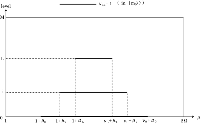
Figure 1: The schematic level scheme and occupation numbers are illustrated.

The quantity $\sigma_{i}$ given in the relation (21) is expressed as

$$\sigma_{i}=\left\{\begin{array}[]{ll}\displaystyle\nu_{0}-\nu_{i}\ ,&(i=1,\ 2,\cdots,\ L)\\ \displaystyle\nu_{0}\ ,&(i=L+1,\ L+2,\cdots,\ M)\\ \end{array}\right.$$ (28)

The above relations lead us to

$$\sigma_{1}\leq\sigma_{2}\leq\cdots\leq\sigma_{L}<\sigma_{L+1}=\sigma_{L+2}=\cdots=\sigma_{M}\ (=\nu_{0})\ .$$ (29)

Hereafter, instead of $\{\sigma_{i}\}$, we formulate the minimum weight states by $\{\nu_{i}\}$. With the use of the relation (11) for ${\widetilde{\Lambda}}_{0}$, we obtain $\lambda$ in the form

$$\lambda=\frac{1}{2}\left(\sum_{\mu=1}^{\mu_{0}}1+\sum_{\mu=\nu_{0}+\mu_{0}+1}^{2\Omega}1\right)=\Omega-\frac{1}{2}\nu_{0}\ .$$ (30)

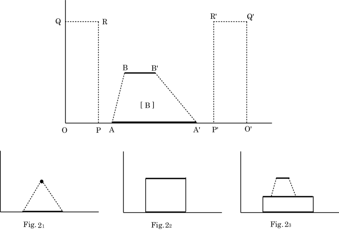
Figure 2: Schematic feature of Fig.1 is depicted.

The total fermion number for $|{m_{0}}\rangle\!\rangle$, which is denoted as $N_{\rm min}$, is given in the form

$$N_{\rm min}=\sum_{i=0}^{L}\nu_{i}=\nu_{0}+\nu(L)\ ,$$

$$\nu(L)=\sum_{i=1}^{L}\nu_{i}\ .$$ (31)

Then, ${\cal L}$, the eigenvalue of ${\widetilde{\cal L}}$ which is defined in the relation (15), is given by

$${\cal L}=\Omega-\frac{M-1}{2(M+1)}\nu_{0}+\frac{1}{M+1}\nu(L)\ .$$ (32)

The quantity $\lambda_{0}$ for any fermion number, $N$, is expressed as

$$\lambda_{0}=\frac{1}{M+1}N-\left(\Omega-\frac{M-1}{2(M+1)}\nu_{0}+\frac{1}{M+1}\nu(L)\right)\ .$$ (33)

Of course, $\lambda_{0}$ obey the inequality

$$-\lambda\leq\lambda_{0}\leq\lambda\ .$$ (34)

The case with $\lambda_{0}=\lambda$ gives us the maximum fermion number, $N_{\rm max}$. With use of the relations (A practical scheme for constructing the minimum weight states of the $su(n)$-Lipkin model in arbitrary fermion number) and (33) for $\lambda_{0}=\lambda$, we have

$$N_{\rm max} = 2\Omega\cdot(M+1)-M\nu_{0}-\nu(L)$$ (35)

$$= N_{\rm min}+(M+1)\cdot 2\lambda\ .$$

Through the relation (23), the normalized state $|{m}\rangle\!\rangle$ is given as

$$|{m}\rangle\!\rangle=\sqrt{\frac{(\lambda-\lambda_{0})!}{(2\lambda)!(\lambda+\lambda_{0})!}}\left({\widetilde{\Lambda}}_{+}\right)^{\lambda+\lambda_{0}}|{m_{0}}\rangle\!\rangle\ .$$ (36)

Therefore, we do not have the trouble to the normalization.

Schematic feature of Fig.1 is depicted in Fig.2. In the upper figure in Fig.2, the block [B] surrounded by the points A, A^′, B and B^′ is trapezoid-like in shape. The segments AA^′ and BB^′ are parallel with each other and the sections AB and A^′B^′ are stepwise. If ${\overline{\rm BB^{\prime}}}=0$ and ${\overline{\rm BB^{\prime}}}={\overline{\rm AA^{\prime}}}$, [B] becomes triangle-like (Fig.2₁) and the rectangular (Fig.2₂), respectively. Further, as a possible shape of [B], we have the figure obtained by piling the trapezoid-like figure on the rectangle (Fig.2₃). The number of the lattice points in [B] corresponds to the total fermion number in $|{m_{0}}\rangle\!\rangle$, $N_{\rm min}$. Intervals OP and P^′O^′ are related with the number of times of the operation of ${\widetilde{\Lambda}}_{+}$. If ${\overline{\rm OA}}\ ({\overline{\rm A^{\prime}O^{\prime}}})=0$, the point P (P^′) disappears and the operation of ${\widetilde{\Lambda}}_{+}$ is meaningless. If ${\overline{\rm OA}}\ ({\overline{\rm A^{\prime}O}})\geq 1$, the interval OP (P^′O^′) for the operation of ${\widetilde{\Lambda}}_{+}$ becomes meaningful. Next, we consider the case composed of two blocks [B¹] and [B²], which is depicted in Fig.3. The discussion in the case with [B] can be applied to the sides OA₁ and A${}^{\prime}_{2}$O^′ in the present case. Then, it may be enough to discuss the interrelation between the points A${}^{\prime}_{1}$ and A₂. It is easily verified that if ${\overline{{\rm A^{\prime}}_{1}{\rm A}_{2}}}\leq 1$, the interval A${}^{\prime}_{1}$A₂ does not contributes to the operation of ${\widetilde{\Lambda}}_{+}$, but if ${\overline{{\rm A^{\prime}}_{1}{\rm A}_{2}}}>1$, A${}^{\prime}_{1}$A₂ contributes to the operation of ${\widetilde{\Lambda}}_{+}$.

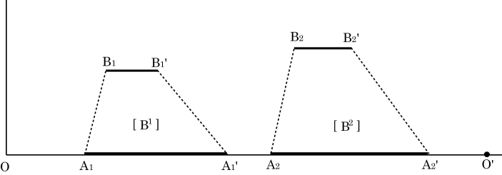
Figure 3: The case composed of two blocks is depicted schematically.

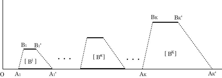
Figure 4: The case composed of $K$ blocks is depicted schematically.

If we follow the above consideration, it may be easy to treat the general case, i.e., the case with $K$ blocks. First, we prepare the blocks labeled by $\kappa=1,\ 2,\cdots,\ K$ and [F^κ] denotes the $\kappa$-th block. Then, it is enough to line them up along the $\mu$-axis (Fig.4). Of course, it is natural to avoid overlapping with each other. The relation (A practical scheme for constructing the minimum weight states of the $su(n)$-Lipkin model in arbitrary fermion number) is useful in the present case and, then, we can construct $|{m_{0}}\rangle\!\rangle$. The relation (36) gives us $|{m}\rangle\!\rangle$. The number of the lattice points $N^{\kappa}$ in [B^κ] and $N_{\rm min}\ (=\sum_{\kappa=1}^{K}N^{\kappa})$ are given by

$$N_{\rm min}=\nu_{0}+\nu(L)\ ,$$ (37)

$$\nu_{0}=\sum_{\kappa=1}^{K}\nu_{0}^{\kappa}\ ,\qquad\nu_{i}=\sum_{\kappa=1}^{K}\nu_{i}^{\kappa}\ ,\qquad\nu(L)=\sum_{i=1}^{L}\nu_{i}\ ,$$ (38)

$$L={\rm max}(L^{1},\cdots,L^{K})\ .$$ (39)

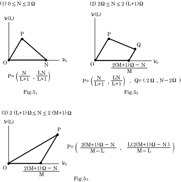
Figure 5: The domains in which the inequalities (24a) and (34) are realized are shown as the area inside the triangle and quadrilateral, respectively.

For the other relations, we have the same expressions as those given in the simplest example.

We will show the domains on the plane $(\nu_{0},\nu(L))$, where the inequalities (24a) and (34) are realized. These inequalities lead us to the following relations:

$$\nu(L)\leq L\nu_{0}\ ,$$ (40a)

$$\nu(L)\leq N-\nu_{0}\ ,$$ (40b)

$$\nu(L)\geq-(2(M+1)\Omega-N)+M\nu_{0}\ .$$ (40c)

The relation (40a) is derived from the inequalities (24a), but the reverse is not true. In the case with $L=0$, simply we can show the following domains:

$$({\rm i})\ \ 0\leq N\leq 2\Omega\ ,\qquad 0\leq\nu_{0}\leq N\ ,\qquad\nu(0)=0\ ,$$ (41a)

$$({\rm ii})\ 2\Omega\leq N\leq 2(M+1)\Omega\ ,\qquad 0\leq\nu_{0}\leq\frac{2(M+1)\Omega-N}{M}\ ,\qquad\nu(0)=0\ .\ \ \ \$$ (41b)

In the case with $1\leq L\leq M-1$, the domains are depicted in Figs. $5_{1}$, $5_{2}$ and $5_{3}$.

Finally, we will give a remark. As was mentioned in the introductory part, the algebraic approach to many-body theories starts in the task how to express the minimum weight states. In this paper, we presented a practical scheme for constructing the minimum weight states in the space spanned by $i=0,\ 1,\cdots,\ M$ and $\mu=1,\ 2,\cdots,\ 2\Omega$. If we encounter the system which contains the components violating the $su(n)$-symmetry in a greater or less degree, we must treat plural minimum weight states simultaneously. In such situations, our scheme may be useful. On the other hand, we know the case where it may be enough to adopt a single minimum weight state. In this case, our scheme becomes much simpler. It may be permitted to change the numbering of $\mu$ appropriately. It suggests us to put $\mu_{i}=0$ $(i=0,\ 1,\cdots,\ L)$ in Fig.1 and it becomes Fig.6. In this case, $|{m_{0}}\rangle\!\rangle$ can be expressed in the form

$$|{m_{0}}\rangle\!\rangle=\prod_{i=0}^{L}\prod_{\mu=1}^{\nu_{i}}{\tilde{c}}_{i,\mu}^{*}|{0}\rangle\!\rangle\ .$$ (42)

The form (42) is useful for the Hamiltonian expressed in terms of the generators (A practical scheme for constructing the minimum weight states of the $su(n)$-Lipkin model in arbitrary fermion number), for example, such as that given in the relations (I.2.6) and (I.2.9).

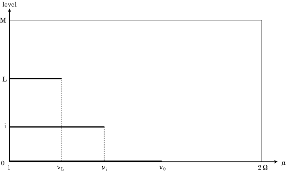
Figure 6: The schematic level scheme and occupation numbers are illustrated.

Thus, we were able to obtain the minimum weight states $|{m}\rangle\!\rangle$ in a practical scheme. Needless to say, the above treatment is predicted on the property of the one-fermion transfer proper to the generators in the $su(n)$-Lipkin model. In this transfer, the quantum number $\mu$ does not change. Further, we should stress that the auxiliary $su(2)$-algebra also plays a central role: With the aid of this algebra, $|{m}\rangle\!\rangle$ is derived from $|{m_{0}}\rangle\!\rangle$.

In the forthcoming paper, we will propose an idea of the random phase approximation based on the minimum weight state (42) and discuss the phase change observed under this approximation.

References

• [1] H. J. Lipkin, N. Meshkov and A. Glick, Nucl. Phys. 62, 188 (1965).
• [2] S. Li, A. Klein and R. M. Dreizler, J. Math Phys. 11, 975 (1970).
N. Meshkov, Phys. Rev. C 3, 2214 (1971).
S. Okubo, J. Math. Phys. 16, 528 (1975).
A. Klein, Nucl. Phys. A 347, 3 (1980).
• [3] Y. Tsue, C. ProvidΓͺncia, J. da ProvidΓͺncia and M. Yamamura, Prog. Theor. Exp. Phys. 2016, 083D03 (2016).
• [4] Y. Tsue, C. ProvidΓͺncia, J. da ProvidΓͺncia and M. Yamamura, Prog. Theor. Exp. Phys. 2016, 083D04 (2016).
• [5] Y. Tsue, C. ProvidΓͺncia, J. da ProvidΓͺncia and M. Yamamura, to appera in Prog. Theor. Exp. Phys. 2017.
• [6] Y. Tsue, C. ProvidΓͺncia, J. da ProvidΓͺncia and M. Yamamura, Prog. Theor. Exp. Phys. 2015, 063D01 (2015).