Spectral discretization errors in filtered subspace iteration

Abstract.

We consider filtered subspace iteration for approximating a cluster of eigenvalues (and its associated eigenspace) of a (possibly unbounded) selfadjoint operator in a Hilbert space. The algorithm is motivated by a quadrature approximation of an operator-valued contour integral of the resolvent. Resolvents on infinite dimensional spaces are discretized in computable finite-dimensional spaces before the algorithm is applied. This study focuses on how such discretizations result in errors in the eigenspace approximations computed by the algorithm. The computed eigenspace is then used to obtain approximations of the eigenvalue cluster. Bounds for the Hausdorff distance between the computed and exact eigenvalue clusters are obtained in terms of the discretization parameters within an abstract framework. A realization of the proposed approach for a model second-order elliptic operator using a standard finite element discretization of the resolvent is described. Some numerical experiments are conducted to gauge the sharpness of the theoretical estimates.

1. Introduction

The goal of this study is to provide an analysis of discretization errors when a subspace iteration algorithm is employed to compute eigenvalues of selfadjoint partial differential operators. Instead of a specific differential operator, we consider a general linear, closed, selfadjoint operator $A:\mathop{\mathrm{dom}}(A)\subseteq{\mathcal{H}}\to{\mathcal{H}}$ (not necessarily bounded) in a complex Hilbert space ${\mathcal{H}}$, whose (real) spectrum is denoted by $\Sigma(A)$. We are interested in computationally approximating a subset $\Lambda$ of the spectrum that consists of a finite collection of eigenvalues of finite multiplicity. Filtered subspace iteration, a natural generalization of the power method, for approximating $\Lambda$ and its corresponding eigenspace (invariant subspace) is roughly described as follows. First, the eigenspace of the cluster $\Lambda$ is transformed to the dominant eigenspace of another, bounded operator called the “filter.” Next, a subspace iteration is applied using the bounded filter. Starting with an initial subspace (usually chosen randomly), the bounded operator is repeatedly applied to it, generating a sequence of subspaces that approximates the eigenspace of $\Lambda$. Approximations of $\Lambda$ are obtained from the approximate eigenspaces by a Rayleigh-Ritz procedure. To apply this filtered subspace iteration in practice requires finite rank approximations of the resolvent at a few points along a contour, obtained by some discretization process, and it is the errors incurred by such discretizations that are investigated here.

The exact eigenspace, namely the span of all the eigenvectors associated with elements of $\Lambda$, is denoted by $E$. Then $m=\dim E,$ being the sum of multiplicities of each element of $\Lambda$, is finite, and we assume $m\geq 1.$ Throughout this paper, the multiplicity $\ell$ of an eigenvalue $\lambda$ of an operator refers to its algebraic multiplicity, i.e., $\lambda$ is a pole of order $\ell$ of the resolvent of that operator. Recall that, for a selfadjoint operator $A$, the algebraic multiplicity of $\lambda$ coincides with its geometric multiplicity, $\dim\ker(\lambda-A)$.

As mentioned above, the idea behind filtered subspace iteration is to transform $E$ into the dominant eigenspace of certain filter operators. We shall see in the next section that the construction of these filters can be motivated by approximations of a Dunford-Taylor contour integral. There has been a resurgence of interest in contour integral methods for eigenvalues due to their excellent parallelizability [2, 4, 15, 24, 14]. Following [2], we identify two different classes of methods in the existing literature that use contour integrals for computation of a targeted cluster of matrix eigenvalues. One class of methods, that often goes by the name SSM [24] (see also [4, 16]), approximates $\Lambda$ by the eigenvalues of a system of moment matrices based on contour integrals. The moment matrices are obtained by approximating the integrals by a quadrature, and the spectral approximation error depends on the accuracy of the quadrature.

The other class of methods, more related to our present contribution, in that they apply filtered subspace iterations to matrices, are referred to by the name FEAST [21] (see also [14, 28]). These algorithms also use quadratures to approximate a contour integral, but the eigenvalues are approximated by a Rayleigh-Ritz procedure using the original matrix. In our view, the use of quadratures in such algorithms is essentially different from their use in SSM-like approaches. Quadratures in FEAST are only used to develop the filter used in a subspace iteration. A consequence of this is that the quadrature error is not as relevant in FEAST as in SSM. The analysis in this paper will show this in precise terms.

When $A$ is a differential operator on an infinite-dimensional space, some approximations to bring the computations into finite-dimensional spaces are necessary. The central concern in this paper is the study of how these approximations affect the final spectral approximations that filtered subspace iteration yields asymptotically. The main technical difficulty in analyzing discretization errors for the unbounded operator eigenproblem is that many of the existing standard tools [3] (applicable for compact operators) are not directly applicable to our situation. We present an abstract framework that allows one to study approximation of spectral clusters of unbounded selfadjoint operators with compact resolvent. Very general discretizations are allowed through a set of abstract assumptions.

To quickly outline the approximation approach studied in this paper, recall that the spectral projector onto $E$, which we denote by $S$, is characterized by a Dunford-Taylor contour integral of the resolvent $R(z)$. Its $N$-term quadrature approximation is denoted by $S_{N}$. In the expression defining $S_{N}$, when $R(z)$ is replaced by a computable finite-rank approximation $R_{h}(z)$, we obtain $S_{N}^{h}$, a practically computable filter. Here $h$ is some discretization parameter (such as the grid spacing) inversely related to a computational finite-dimensional space. By repeated application of $S_{N}^{h}$, the iteration produces a sequence of subspaces $\{\smash{{E_{h}^{({\ell})}}}:\ell=1,2,\ldots\}$, which we study. Due to the approximations, it is not obvious if the iterates $\smash{{E_{h}^{({\ell})}}}$ converge to some limit $E_{h}$. We begin our analysis by showing that they do under certain sufficient conditions, after which we focus on analyzing the limit.

To summarize the novelty of this work, this is the first work to study the effect of the discretization parameter $h$ (in addition to $N$). The errors in eigenspace approximations often need to be measured in stronger norms than the base ${\mathcal{H}}$-norm. The example of elliptic differential operators on ${\mathcal{H}}=L^{2}(\varOmega)$ illustrates the need to measure eigenfunction errors in a stronger norm like the $H^{1}(\varOmega)$-norm. To our knowledge, this is the first work to give bounds for eigenspace discretization errors in ${\mathcal{H}}$-norm as well as a stronger ${\mathcal{V}}$-norm. We provide the first result showing that the Hausdorff distance between the eigenvalue cluster computed by filtered subspace iteration and $\Lambda$ converges to zero at predictable rates as the discretization parameter $h\to 0$. To highlight one more conclusion from our analysis, increasing $N$ has little effect on the spectral discretization error as measured by the gap between $E$ and $E_{h}$ (although it may affect [7] the speed of convergence of the filtered subspace iteration to $E_{h}$).

The rest of the paper is organized as follows. In Section 2, we describe precisely the above-mentioned process of double approximation (going from $S$ to $S_{N}^{h}$) and introduce the necessary assumptions for the error analysis. Section 3 introduces the space to which filtered subspace iteration using $S_{N}^{h}$ converges. Bounds for the gap between computed and exact eigenspaces are proved in Section 4. Eigenvalue errors are then bounded using the square of this gap. Analysis of a standard finite element discretization of the resolvent of a model operator in Section 6 provides an example of how abstract conditions on the resolvent might be verified in practice. The practical performance of the algorithm with the discretization is reported in Section 7.

2. Preliminaries

Let $A$, $\Lambda$ and $E$ be as discussed previously. As already mentioned, filters are linear operators on ${\mathcal{H}}$ having $E$ as their dominant eigenspace, in the sense made precise below.

Suppose that $\Gamma\subset\mathbb{C}\setminus\Sigma(A)$ is a positively oriented, simple, closed contour that encloses $\Lambda$ and excludes $\Sigma(A)\setminus\Lambda$, and let $G\subset\mathbb{C}$ be the open set whose boundary is $\Gamma$. By the Cauchy Integral Formula,

(1) $$r(\xi)=\frac{1}{2\pi\mathrm{i}}\oint_{\Gamma}(z-\xi)^{-1}\,dz=\begin{cases}1,&\,\xi\in G,\\ 0,&\xi\in\mathbb{C}\setminus(G\cup\Gamma).\end{cases}$$

Thus $r(\xi)$ equals a.e. the indicator function of $G$ in $\mathbb{C}$. The associated (orthogonal) spectral projection $S:{\mathcal{H}}\to{\mathcal{H}}$ is the bounded linear operator given by the Dunford-Taylor integral

(2) $$S=\frac{1}{2\pi\mathrm{i}}\oint_{\Gamma}R(z)\,dz,$$

where $R(z)=(z-A)^{-1}$ is the resolvent, a bounded linear operator on ${\mathcal{H}}$ for each $z\in\Gamma$. Since $\Gamma$ encloses $\Lambda$ and no other element of $\Sigma(A)$, its well known that

(3) $$E=\mathop{\mathrm{ran}}(S).$$

Furthermore, by functional calculus (see [22, Theorem VIII.5], [26, Theorem 5.9] or [5, Section 6.4]), if $(\lambda,\phi)\in\Sigma(A)\times\mathop{\mathrm{dom}}(A)$ satisfies $A\phi=\lambda\phi$, then $S\phi=r(A)\phi=r(\lambda)\phi$. Since $r(\lambda)$ equals $1$ for all $\lambda\in\Lambda$ and equals $0$ for all other elements of $\Sigma(A)$, the desired eigenspace $E$ of $A$ is now the dominant eigenspace of $S=r(A)$. In this sense, $S$ is an ideal filter.

Motivated by quadrature approximations of (1), in the same spirit as [4, 13, 21, 28, 24], we approximate $r(\xi)$ by

(4) $$r_{N}(\xi)=w_{N}+\sum_{k=0}^{N-1}w_{k}(z_{k}-\xi)^{-1}~{},$$

for some $w_{k},z_{k}\in\mathbb{C}.$ The corresponding rational filter is the operator

(5) $$S_{N} =r_{N}(A)=w_{N}+\sum_{k=0}^{N-1}w_{k}R(z_{k}),$$

which can be viewed as an approximation of $S$. It is common to refer to $S_{N}$, as well as the rational function $r_{N}(\xi)$, as the filter. As in the case of $S$, if $(\lambda,\phi)\in\Sigma(A)\times\mathop{\mathrm{dom}}(A)$ satisfies $A\phi=\lambda\phi$, then $S_{N}\phi=r_{N}(\lambda)\phi$. In particular, the set $\Lambda$ of eigenvalues of interest have been mapped to $\{r_{N}(\lambda):\lambda\in\Lambda\}$ by the filter.

These mapped eigenvalues are dominant eigenvalues of $S_{N}$ if

(6) $$\min_{\lambda\in\Lambda}|r_{N}(\lambda)|>\sup_{\mu\in\Sigma(A)\setminus\Lambda}|r_{N}(\mu)|$$

holds. This dominance can be obtained provided $\Lambda$ is strictly separated from the remainder of the spectrum. To quantify the separation, we consider the following strictly separated subsets of $\mathbb{R}$ centered around $y\in\mathbb{R}$

$$I_{\gamma}^{y}=\{x\in\mathbb{R}:|x-y|\leq\gamma\},\qquad O_{\delta,\gamma}^{y}=\{x\in\mathbb{R}:|x-y|\geq(1+\delta)\gamma\}.$$

for some positive numbers $\gamma$ and $\delta$. If the spectral cluster of interest is within $I_{\gamma}^{y}$, then the number $\delta$ provides a measure of the relative gap between it and the rest of the spectrum—relative to the radius $\gamma$ of the interval wherein we seek eigenvalues. Using the numbers $y,\gamma,$ and $\delta$, define

(7) $$W=\sum_{k=0}^{N}|w_{k}|,\quad\quad\hat{\kappa}=\frac{\displaystyle\sup_{x\in O_{\delta,\gamma}^{y}}|r_{N}(x)|}{\displaystyle\inf_{x\in I_{\gamma}^{y}}|r_{N}(x)|}.$$

These definitions help us to formulate the following assumption on the filter and cluster separation.

Assumption 1.

We assume there are $y\in\mathbb{R}$, $\delta>0$ and $\gamma>0$ such that

(8) $$\Lambda\subset I_{\gamma}^{y},\qquad\Sigma(A)\setminus\Lambda\subset O_{\delta,\gamma}^{y}.$$

We assume that $r_{N}$ is a rational function of the form (4) with the property that $z_{k}\notin\overline{\Sigma(A)},$ $W<\infty$, and $\hat{\kappa}<1$.

Note that if $\hat{\kappa}<1$, then (6) holds. When an $N$-point trapezoidal rule is used for quadrature approximation we obtain an $r_{N}$ as in (4) with $w_{N}=0$. When the Zolotarev rational approximation of $r(\xi)$ is used to construct $r_{N}$, the term $w_{N}$ is nonzero [14]. In Section 7, we shall use the so-called Butterworth filter which is obtained by setting $w_{N}=0$ and for $k=0,\ldots,N-1$,

(9) $$z_{k}=\gamma e^{\mathrm{i}(\theta_{k}+\phi)}+y,\quad\quad w_{k}=\gamma e^{\mathrm{i}(\theta_{k}+\phi)}/N.$$

with $\theta_{k}=2\pi k/N$ and $\phi=\pm\pi/N.$ This filter as well as several other examples of $r_{N}$ satisfying Assumption 1 are studied in [7].

Next, we introduce a subspace ${\mathcal{V}}\subseteq{\mathcal{H}}$, motivated by the need to prove results that bound discretization errors in norms stronger than the ${\mathcal{H}}$-norm. We place the following assumption and give example classes of operators where the assumption holds.

Assumption 2.

Suppose there is a Hilbert space ${\mathcal{V}}\subseteq{\mathcal{H}}$ such that $E\subseteq{\mathcal{V}}$, there is a $C_{\mathcal{V}}>0$ such that for all $u\in{\mathcal{V}}$, $\|u\|_{\mathcal{H}}\leq C_{\mathcal{V}}\|u\|_{\mathcal{V}}$, and ${\mathcal{V}}$ is an invariant subspace of $R(z)$.

Example 2.1 (${\mathcal{V}}$ is the whole space).

Set ${\mathcal{V}}={\mathcal{H}}$, with $(\cdot,\cdot)_{\mathcal{V}}=(\cdot,\cdot)_{\mathcal{H}}$. In this case it is obvious that all statements of Assumption 2 hold.  $\Box$

Example 2.2 (${\mathcal{V}}$ is the domain of a positive form).

Suppose $a(u,v)$ is a densely defined closed sesquilinear Hermitian form on ${\mathcal{H}}$ and there is a $\delta>0$ such that

(10) $$a(v,v)\geq\delta\|v\|_{{\mathcal{H}}}^{2},\qquad v\in\mathop{\mathrm{dom}}(a).$$

Set

$${\mathcal{V}}=\mathop{\mathrm{dom}}(a),\qquad\|v\|_{\mathcal{V}}=a(v,v)^{1/2}.$$

To show that Assumption 2 holds in this case, first set the operator $A$ to be the closed selfadjoint operator associated with the form, namely it satisfies $a(u,v)=(Au,v)$ for all $u\in\mathop{\mathrm{dom}}(A)\subseteq\mathop{\mathrm{dom}}(a)$ and all $v\in\mathop{\mathrm{dom}}(a)$ (see the first representation theorem [18, TheoremVI.2.1] or [26, Theorem 10.7]). Note that, in this case, $A$ is a positive operator. Hence $A$ has a unique selfadjoint positive square root [18, Theorem V.3.35], denoted by $A^{1/2}$, that commutes with any bounded operator that commutes with $A$. By the second representation theorem [18, Theorem VI.2.23], the form domain is characterized by $\mathop{\mathrm{dom}}(a)=\mathop{\mathrm{dom}}(A^{1/2})$, and $\|v\|_{\mathcal{V}}=\|A^{1/2}v\|_{\mathcal{H}}$ for $v\in{\mathcal{V}}$. The strict positivity of $a$ ensures that both $A$ and $A^{1/2}$ are invertible on their respective domains.

Since $a$ is closed, ${\mathcal{V}}$ is complete. Due to (10), ${\mathcal{V}}$ is continuously embedded in ${\mathcal{H}}$, with the constant $C_{\mathcal{V}}=\delta^{-1/2}$. The exact eigenspace $E$ is contained in $\mathop{\mathrm{dom}}(A)\subseteq\mathop{\mathrm{dom}}(A^{1/2})={\mathcal{V}}$. Since $A^{1/2}$ and $A^{-1/2}$ commutes with $R(z)$, for any $v,w\in{\mathcal{V}}$, we have for any $v\in{\mathcal{V}}=\mathop{\mathrm{dom}}(A^{1/2})$ and $z$ in the resolvent set of $A$,

$$R(z)v =(z-A)^{-1}v=A^{-1/2}(z-A)^{-1}A^{1/2}v~{}.$$

Since $\mathop{\mathrm{ran}}(A^{-1/2})=\mathop{\mathrm{dom}}(A^{1/2})={\mathcal{V}}$, we see that $R(z){\mathcal{V}}\subseteq{\mathcal{V}}$. Thus Assumption 2 is verified.  $\Box$

Example 2.3 (${\mathcal{V}}$ is a graph space).

Given $A$, put ${\mathcal{V}}=\mathop{\mathrm{dom}}(A)\subseteq{\mathcal{H}}$ and endow the set ${\mathcal{V}}$ with the topology of the graph norm

$$\|v\|_{{\mathcal{V}}}=\left(\|v\|_{{\mathcal{H}}}^{2}+\|Av\|_{{\mathcal{H}}}^{2}\right)^{1/2},\qquad v\in{\mathcal{V}}.$$

We claim that Assumption 2 holds in this case. Indeed, since $A$ is closed, the graph norm makes ${\mathcal{V}}$ into a Hilbert space. Obviously $E\subset{\mathcal{V}}$ and ${\mathcal{V}}$ is continuously embedded into ${\mathcal{H}}$ with $C_{\mathcal{V}}=1$. Since $A$ commutes with $R(z)$ for any $z$ in the resolvent set of $A$, we have $R(z)\mathop{\mathrm{dom}}(A)\subseteq\mathop{\mathrm{dom}}(A)$.  $\Box$

The next essential ingredient in our study is the approximation of $R(z)$. When $A$ is a differential operator on an infinite-dimensional space, to obtain numerical spectral approximations, we perform a discretization to approximate the resolvent of $A$ in a computable finite-dimensional space. Accordingly, let ${\mathcal{V}}_{h}$ be a finite-dimensional subspace of ${\mathcal{V}}$, where $h$ is a parameter inversely related to the finite dimension, e.g., a mesh size parameter $h$ that goes to $0$ as the dimension increases. Let $R_{h}(z):{\mathcal{H}}\to{\mathcal{V}}_{h}$ be a finite-rank approximation to the resolvent $R(z)$ satisfying the following assumption.

Assumption 3.

Assume that the operators $R_{h}(z_{k})$ and $R(z_{k})$ are bounded in ${\mathcal{V}}$ and satisfy

(11) $$\lim_{h\to 0}\|R_{h}(z_{k})-R(z_{k})\|_{{\mathcal{V}}}=0$$

for all $k=0,1,\ldots,N-1$.

Note that this assumption implies that $R(z_{k})$, being the limit of finite-rank operators, is compact in ${\mathcal{V}}$. Its also compact as an operator on ${\mathcal{H}}$ due to Assumption 2. Consequently $R(z)$ is compact for all $z$ in the resolvent set. Relaxing Assumption 3 to go beyond operators with compact resolvent is outside the scope of the current work.

Consider the approximation of $S_{N}$ given by

(12) $$S^{h}_{N} =w_{N}+\sum_{k=0}^{N-1}w_{k}R_{h}(z_{k}).$$

In view of Assumption 3, we shall from now on view both $S_{N}$ and $S_{N}^{h}$ as bounded operators on ${\mathcal{V}}$. Note that $S_{N}^{h}$ need not be selfadjoint. In Section 6, we shall consider an example of $S_{N}^{h},$ obtained by a standard finite element discretization of $R(z)$ based on symmetrically located $z_{k}$, that is selfadjoint. But in general $S_{N}^{h}$ may fail to be selfadjoint due to the configuration of $\{z_{k}\}$ or due to the properties of the discretization (see e.g., [8]).

With the resolvent discretization, filtered subspace iteration can be described mathematically in very simple terms. Namely, starting with a subspace ${E_{h}^{({0})}}\subseteq{\mathcal{V}}_{h}$, compute

(13) $${E_{h}^{({\ell})}}=S^{h}_{N}{E_{h}^{({\ell-1})}},\qquad\text{ for }\ell=1,2,\ldots.$$

Of course, in practice, one must include (implicit or explicit) normalization steps and maintain a basis for the spaces $\smash{{E_{h}^{({\ell})}}}$, but these details are immaterial in our ensuing analysis. The convergence of the FEAST algorithm in Euclidean ($\ell^{2}$ and matrix-based) norms was previously studied in [14, 23]. In Section 3, we shall utilize some of their ideas to show that (13) converges in ${\mathcal{V}}$, despite the perturbations caused by the above-mentioned resolvent approximations. Further studies on iterative speed of convergence of (13) may be found in [7]. Here however, we are solely interested in studying the discretization errors found in the final asymptotic product of the algorithm, i.e., the discretization errors in what the algorithm outputs as the “limit space” when (13) converges.

3. The limit space

The purpose of this section is to identify to what space convergence of (13) might happen. We also briefly examine in what sense $\smash{{E_{h}^{({\ell})}}}$ converges to it.

In view of Assumption 2, ${\mathcal{V}}$ is an invariant subspace of the resolvent. Hence in the remainder of the paper, we will proceed viewing $S_{N}$ and $S_{N}^{h}$ as operators on ${\mathcal{V}}$. To measure the distance between two linear subspaces $M$ and $L$ of ${\mathcal{V}}$, we use the standard notion of gap [18] defined by

(14) $$\operatorname{gap}_{\mathcal{V}}(M,L)=\max\left[\sup_{m\in U_{M}^{\mathcal{V}}}\mathop{\textstyle{\mathrm{dist}_{{{\mathcal{V}}}}}}(m,L),\;\sup_{l\in U_{L}^{\mathcal{V}}}\mathop{\textstyle{\mathrm{dist}_{{{\mathcal{V}}}}}}(l,M)\right].$$

Here and throughout, for any linear subspace $M\subseteq{\mathcal{V}}$, we use $U_{M}^{\mathcal{V}}$ to denote its unit ball $\{w\in M:\;\|w\|_{\mathcal{V}}=1\}$.

Recall that $E=\mathop{\mathrm{ran}}S$, the exact eigenspace corresponding to eigenvalues $\lambda_{1},\ldots,\lambda_{m}$ of $A$ that we wish to approximate. If Assumption 1 holds, then the operator $S_{N}=r_{N}(A)$ has dominant eigenvalues

$$\mu_{i}=r_{N}(\lambda_{i}),\qquad i=1,2,\ldots,m,$$

strictly separated in absolute value from the remainder of $\Sigma(S_{N})$. In particular, since $\hat{\kappa}<1$, we have $\mu_{i}\neq 0$ for $i\leq m$, and letting $\mu_{*}=\sup\{|\mu|:\mu\in\Sigma(S_{N})\setminus\{\mu_{1},\ldots\mu_{m}\}\}$,

(15) $$\mu_{*}<|\mu_{i}|,\quad i=1,2,\ldots,m.$$

In view of these facts, we can find a simple rectifiable curve $\Theta$ in the complex plane that encloses $\{\mu_{1},\ldots,\mu_{m}\}$ and lies strictly outside the circle of radius $\mu_{*}$. In particular, $\Theta$ encloses no other element of $\Sigma(S_{N})$. Define the spectral projector of $S_{N}$ by

$$P_{N}=\frac{1}{2\pi\mathrm{i}}\oint_{\Theta}(z-S_{N})^{-1}\,dz.$$

Then $E_{N}=\mathop{\mathrm{ran}}P_{N}$ is the eigenspace of $S_{N}$ corresponding to its eigenvalues $\mu_{1},\ldots,\mu_{m}$.

Lemma 3.1.

We have $E_{N}=E$ and $P_{N}=S$.

Proof.

Since $\dim E_{N}=\dim E=m$, it suffices to prove that $E\subseteq E_{N}$. If $e_{i}\in E$ is an eigenfunction of $A$ corresponding to the eigenvalue $\lambda_{i}\in\Lambda$, then $S_{N}e_{i}=r_{N}(\lambda_{i})e_{i}$, so $e_{i}\in E_{N}$. Since $P_{N}$ and $S$ are both orthogonal projectors and have the same range, they are the same operator. ∎

Next, observe that when Assumption 3 is used after subtracting the expression for $S_{N}^{h}$ in (12) from that of $S_{N}$, we obtain

(16) $$\|S_{N}-S^{h}_{N}\|_{\mathcal{V}} \leq W\max_{k=0,\ldots,N-1}\|R_{h}(z_{k})-R(z_{k})\|_{{\mathcal{V}}}\to 0$$

as $h$ goes to 0. Let us recall the standard ramifications of the convergence of operators in norm given by (16) (see e.g., [18, Theorem IV.3.16] or [1]). Namely, given an open disc enclosing an isolated eigenvalue of $S_{N}$ of multiplicity $\ell$, (16) implies that for sufficiently small $h$, there are exactly $\ell$ eigenvalues (counting multiplicities) of $S^{h}_{N}$ in the same disc. In particular, this implies that, for sufficiently small $h$, the contour $\Theta$ is in the resolvent set of $S^{h}_{N}$ and encloses exactly $m$ eigenvalues (counting multiplicities) of $S^{h}_{N}$, which we shall enumerate as $\mu_{1}^{h},\mu_{2}^{h},\ldots,\mu_{m}^{h}$. Hence, the integral

$$P_{h}=\frac{1}{2\pi\mathrm{i}}\oint_{\Theta}\left(z-S^{h}_{N}\right)^{-1}\,dz$$

is well defined.

Definition 3.2.

Let $E_{h}=\mathop{\mathrm{ran}}P_{h}$.

Clearly, $P_{h}$ is the spectral projector of $S^{h}_{N}$ corresponding to the eigenvalues $\mu_{1}^{h},\mu_{2}^{h},\ldots,\mu_{m}^{h}$. Hence,

(17) $$\dim E_{h}=m.$$

Note also that by construction of $\Theta,$

(18) $$\mu^{h}_{i}\neq 0,\qquad i=1,2,\ldots,m.$$

We now show that the above-defined $E_{h}$ is the limit space of subspace iterates $E_{h}^{(\ell)}$.

Theorem 3.3.

Starting with a subspace ${E_{h}^{({0})}}\subseteq{\mathcal{V}}_{h}$ satisfying $\dim({E_{h}^{({0})}})=\dim(P_{h}{E_{h}^{({0})}})=m$, we compute ${E_{h}^{({\ell})}}$ by (13). Suppose Assumptions 1–3 hold. Then there is an $h_{0}>0$ such that, for all $h<h_{0}$,

$$\lim_{\ell\to\infty}\operatorname{gap}_{\mathcal{V}}({E_{h}^{({\ell})}},E_{h})=0.$$

Proof.

Step 1: Recall from (17) that $\dim(E_{h})=m$ for sufficiently small $h$. Together with $P_{h}{E_{h}^{({0})}}\subseteq E_{h}$ and the assumption $\dim(P_{h}{E_{h}^{({0})}})=m$, this leads to the equality

(19) $$P_{h}{E_{h}^{({0})}}=E_{h}.$$

Thus

$$P_{h}{E_{h}^{({\ell})}}=P_{h}(S^{h}_{N})^{\ell}{E_{h}^{({0})}}=(S^{h}_{N})^{\ell}P_{h}{E_{h}^{({0})}}=(S^{h}_{N})^{\ell}E_{h}=E_{h}.$$

In particular, this implies that $\dim({E_{h}^{({\ell})}})\geq\dim(P_{h}{E_{h}^{({\ell})}})=\dim(E_{h})$. Hence,

(20) $$\dim({E_{h}^{({\ell})}})=\dim(E_{h})=m,\qquad\ell=0,1,2,\ldots.$$

Step 2: Let $v_{i}$ be an eigenvector of $S_{N}^{h}$ corresponding to eigenvalue $\mu^{h}_{i}$. We shall now find an approximant of $v_{i}$ in $E_{h}^{(\ell)}$. Due to (19), there is a $q_{i}^{\!({{0}})}$ in ${E_{h}^{({0})}}$ such that $P_{h}q_{i}^{\!({{0}})}=v_{i}$. Set

$$q_{i}^{\!({{\ell}})}=\left(\frac{1}{\mu^{h}_{i}}\right)^{\ell}(S_{N}^{h})^{\ell}\,q_{i}^{\!({{0}})}.$$

Clearly $q_{i}^{\!({{\ell}})}$ is well defined due to (18) and is in ${E_{h}^{({\ell})}}$. Moreover,

$$v_{i}-q_{i}^{\!({{\ell}})} =v_{i}-\mu_{i}^{-\ell}(S_{N}^{h})^{\ell}\big{[}P_{h}q_{i}^{\!({{0}})}+(I-P_{h})q_{i}^{\!({{0}})}\big{]}$$

$$=-\mu_{i}^{-\ell}(S_{N}^{h})^{\ell}(I-P_{h})q_{i}^{\!({{0}})},$$

Since $(I-P_{h})q_{i}^{\!({{0}})}=(I-P_{h})^{2}q_{i}^{\!({{0}})}=(I-P_{h})(q_{i}^{\!({{0}})}-v_{i})$, we conclude that

(21) $$v_{i}-q_{i}^{\!({{\ell}})}=-\mu_{i}^{-\ell}(S_{N}^{h})^{\ell}(I-P_{h})(q_{i}^{\!({{0}})}-v_{i}).$$

Step 3: Since $S_{N}^{h}$ commutes with $P_{h}$, equation (21) implies

$$\|v-q_{i}^{\!({{\ell}})}\|_{\mathcal{V}}\leq\frac{1}{|\mu^{h}_{i}|^{\ell}}\left\|\big{[}S_{N}^{h}(I-P_{h})\big{]}^{\ell}\right\|_{\mathcal{V}}\|v-q_{i}^{\!({{0}})}\|_{\mathcal{V}}.$$

Let $\mu_{*}^{h}$ denote the supremum of $|\mu|$ over all $\mu$ in $\Sigma(S_{N}^{h})\setminus\{\mu_{1}^{h},\mu_{2}^{h},\ldots,\mu_{m}^{h}\}$, i.e., $\mu_{*}^{h}$ is the spectral radius of $S_{N}^{h}(I-P_{h})$, so

$$\mu_{*}^{h}=\lim_{\ell\to\infty}\|[S_{N}^{h}(I-P_{h})]^{\ell}\|_{\mathcal{V}}^{1/\ell}.$$

Hence, for any given $\varepsilon>0$, there is an $\ell_{0}\geq 1$ such that $\|[S_{N}^{h}(I-P_{h})]^{\ell}\|_{\mathcal{V}}\leq(\mu_{h}^{*}+\varepsilon)^{\ell}$ holds for all $\ell>\ell_{0}$ and consequently

(22) $$\|v-q_{i}^{\!({{\ell}})}\|_{\mathcal{V}}\leq\frac{(\mu_{*}^{h}+\varepsilon)^{\ell}}{|\mu^{h}_{i}|^{\ell}}\|v-q_{i}^{\!({{0}})}\|_{\mathcal{V}}.$$

Step 4: As already seen, a consequence of Assumptions 1 and 3, is that by making $h$ sufficiently small, we ensure that the eigenvalues $\mu_{1}^{h},\mu_{2}^{h},$ $\ldots,$ $\mu_{m}^{h}$ of $S^{h}_{N}$ are strictly separated in magnitude from the remaining eigenvalues – cf. (15). Hence we may choose an $\varepsilon>0$ so small that $\delta_{i}=(\mu_{*}^{h}+\varepsilon)/|\mu_{i}^{h}|<1.$ Then, with $\alpha_{i}=\|v_{i}-q_{i}^{\!({{0}})}\|_{\mathcal{V}},$ the estimate (22) implies

(23) $$\|v_{i}-q_{i}^{\!({{\ell}})}\|_{\mathcal{V}}\leq\alpha_{i}\delta_{i}^{\ell},\qquad\ell>\ell_{0}.$$

Note that $v_{i},$ $i=1,\ldots,m$ form a basis for $E_{h}$. Hence, we may expand an arbitrary $v_{h}\in U^{\mathcal{V}}_{E_{h}}$ in this basis and construct an approximation of $v_{h}$ using the same coefficients:

$$v_{h}=\sum_{i=1}^{m}c_{i}v_{i},\qquad q_{\ell}=\sum_{i=1}^{m}c_{i}q_{i}^{(\ell)}.$$

Then, by (23),

(24) $$\mathop{\textstyle{\mathrm{dist}_{{{\mathcal{V}}}}}}(v_{h},{E_{h}^{({\ell})}})\leq\|v_{h}-q_{\ell}\|_{{\mathcal{V}}}\leq\sum_{i=1}^{m}|c_{i}\alpha_{i}|\delta_{i}^{\ell}\leq\alpha\left(\sum_{i=1}^{m}|c_{i}|^{2}\right)^{1/2}\left(\sum_{i=1}^{m}\delta_{i}^{2\ell}\right)^{1/2}.$$

where $\alpha=\max_{i}\alpha_{i}$.

Step 5: Denote one of the two suprema in the definition of $\operatorname{gap}_{\mathcal{V}}(E_{h},{E_{h}^{({\ell})}})$ by

$$\delta_{h,\ell}=\sup_{v_{h}\in U^{\mathcal{V}}_{E_{h}}}\mathop{\textstyle{\mathrm{dist}_{{{\mathcal{V}}}}}}\left(v_{h},{E_{h}^{({\ell})}}\right).$$

Let $g$ denotes the minimal eigenvalue of the $m\times m$ Gram matrix of the $v_{i}$-basis (whose $(i,j)$th entry is $(v_{i},v_{j})_{\mathcal{V}}$). Then $g\sum_{i=1}^{m}|c_{i}|^{2}\leq\|v_{h}\|_{\mathcal{V}}^{2}=1$. (Note that $g$ may depend on $h$, but is independent of $\ell$.) Hence (24) implies $\delta_{h,\ell}^{2}\leq(\alpha^{2}/g)\sum_{i=1}^{m}\delta_{i}^{2\ell}$ which converges to $0$ as $\ell\to\infty$ since $\delta_{i}<1$.

In particular, for large enough $\ell$, we have $\delta_{h,\ell}<1$. Hence, by [18, Theorem I.6.34] there is a subspace $\tilde{E}_{h}^{({\ell})}\subseteq{E_{h}^{({\ell})}}$ such that $\operatorname{gap}_{\mathcal{V}}(E_{h},\tilde{E}_{h}^{({\ell})})=\delta_{h,\ell}<1.$ Hence, $\dim(E_{h})=\dim(\tilde{E}_{h}^{({\ell})})=m$. But by (20), the only subspace $\tilde{E}_{h}^{({\ell})}\subseteq{E_{h}^{({\ell})}}$ of dimension $m$ is $\tilde{E}_{h}^{({\ell})}={E_{h}^{({\ell})}}$. Thus, for sufficiently large $\ell$,

$$\operatorname{gap}_{\mathcal{V}}(E_{h},{E_{h}^{({\ell})}})=\delta_{h,\ell},$$

and the proof is complete since $\delta_{h,\ell}\to 0$ as $\ell\to\infty$. ∎

To summarize this section, we have defined a space $E_{h}$ (in Definition 3.2) using $S_{N}^{h}$, but independently of the filtered subspace iteration (13), and have shown (in Theorem 3.3) that under certain conditions the iteration converges to it. The convergence of FEAST iterations for matrices (disregarding any discretization errors) were previously studied in [14] when ${\mathcal{H}}=\mathbb{R}^{n}$ and $\|\cdot\|_{{\mathcal{V}}}=\|\cdot\|_{{\mathcal{H}}}$ using the theory of subspace iterations [23]. In fact the identity obtained in Step 2 of the above proof was motivated by a standard argument in the analysis of subspace iterations [23]. Our proof of Theorem 3.3 gives a rigorous justification for the intuition that if the discretization is good, then despite the errors in the resolvent approximations, filtered subspace iteration should converge for well-separated eigenvalue clusters.

4. Discretization errors in eigenspace

In this section we study how the discrete eigenspace $E_{h}$ approaches the exact eigenspace $E$ as the discretization parameter $h$ goes to $0$.

Theorem 4.1.

Suppose Assumptions 1–3 hold. Then there is a $C_{N}>0$ and an $h_{0}>0$ such that for all $h<h_{0}$,

(25) $$\operatorname{gap}_{\mathcal{V}}(E,E_{h})\leq C_{N}W\max_{k=1,\ldots,N}\left\|\big{[}R(z_{k})-R_{h}(z_{k})\big{]}\raisebox{-1.00006pt}{$\big{|}_{E}$}\right\|_{\mathcal{V}},$$

so, in particular,

$$\lim_{h\to 0}\operatorname{gap}_{\mathcal{V}}(E,E_{h})=0.$$

Proof.

Consider one of the two suprema in the definition of $\operatorname{gap}_{\mathcal{V}}(E_{N},E_{h})$, namely

(26) $$\delta_{h}=\sup_{e\in U^{\mathcal{V}}_{E_{N}}}\mathop{\textstyle{\mathrm{dist}_{{{\mathcal{V}}}}}}(e,E_{h}).$$

Then,

(27) $$\delta_{h} \leq\sup_{e\in U^{\mathcal{V}}_{E_{N}}}\|e-P_{h}e\|_{\mathcal{V}}\leq\sup_{e\in U^{\mathcal{V}}_{E_{N}}}\|(P_{N}-P_{h})e\|_{\mathcal{V}}.$$

Note that

$$P_{N}-P_{h} =\frac{1}{2\pi\mathrm{i}}\oint_{\Theta}\left[(z-S_{N})^{-1}-(z-S^{h}_{N})^{-1}\right]\,dz$$

$$=\frac{1}{2\pi\mathrm{i}}\oint_{\Theta}(z-S^{h}_{N})^{-1}(S_{N}-S^{h}_{N})(z-S_{N})^{-1}\,dz.$$

Since $E_{N}$ is an invariant subspace of $(z-S_{N})^{-1}$, the above identity gives the estimate

$$\|P_{N}e-P_{h}e\|_{\mathcal{V}} \leq\left[\frac{1}{2\pi}\oint_{\Theta}\|(z-S_{N})^{-1}\|_{\mathcal{V}}\|(z-S^{h}_{N})^{-1}\|_{\mathcal{V}}\,dz\right]\|(S_{N}-S^{h}_{N})|_{E_{N}}\|_{{\mathcal{V}}}\|e\|_{\mathcal{V}}.$$

Returning to (27), we conclude that $\delta_{h}\leq C_{N}\|(S_{N}-S^{h}_{N})|_{E_{N}}\|_{{\mathcal{V}}}$, where $C_{N}$ is a bound for the quantity in square brackets above. Clearly, $C_{N}$ can be bounded independently of $h$, since $\|(z-S_{N}^{h})^{-1}\|_{\mathcal{V}}\to\|(z-S_{N})^{-1}\|_{\mathcal{V}}.$

Thus, by virtue of (16), $\delta_{h}\to 0$ as $h\to 0.$ In particular, for sufficiently small $h$, we have $\delta_{h}<1$. Then, by [18, Theorem I.6.34], there is a closed subspace $\tilde{E}_{h}\subseteq E_{h}$ such that $\operatorname{gap}_{\mathcal{V}}(E_{N},\tilde{E}_{h})=\delta_{h}<1$ and $\dim\tilde{E}_{h}=\dim E_{N}=m$. Because of (17), this implies that $\tilde{E}_{h}=E_{h}$. Since $E_{N}=E$ by Lemma 3.1, we finish the proof of (25) by noting that $\operatorname{gap}_{{\mathcal{V}}}(E,E_{h})=\operatorname{gap}_{\mathcal{V}}(E_{N},\tilde{E}_{h})=\delta_{h}$. ∎

Remark 4.2.

If ${\mathcal{V}}$ is replaced by ${\mathcal{H}}$ in (14), we obtain $\operatorname{gap}_{{\mathcal{H}}}(M,L)$, so

$$\operatorname{gap}_{\mathcal{H}}(E,E_{h})=\max\left[\sup_{e\in U_{E}^{\mathcal{H}}}\mathop{\textstyle{\mathrm{dist}_{{{\mathcal{H}}}}}}(e,E_{h}),\sup_{m\in U_{E_{h}}^{\mathcal{H}}}\mathop{\textstyle{\mathrm{dist}_{{{\mathcal{H}}}}}}(m,E)\right].$$

Its natural to ask if $\operatorname{gap}_{\mathcal{V}}(E,E_{h})\to 0$ implies $\operatorname{gap}_{\mathcal{H}}(E,E_{h})\to 0$ as $h\to 0$. Let $\delta^{\mathcal{H}}_{h}$ denote the first of the two suprema above. Since $E$ is finite-dimensional, there is a $C_{m}>0$ such that $\|e\|_{{\mathcal{H}}}\geq C_{m}\|e\|_{{\mathcal{V}}}$ for all $e$ in $E$. Using also Assumption 2,

$$\delta^{\mathcal{H}}_{h}=\sup_{0\neq e\in E}\frac{\mathop{\textstyle{\mathrm{dist}_{{{\mathcal{H}}}}}}(e,E_{h})}{\|e\|_{{\mathcal{H}}}}\leq\,\frac{C_{\mathcal{V}}}{C_{m}}\,{\sup_{0\neq e\in E}}\frac{\mathop{\textstyle{\mathrm{dist}_{{{\mathcal{V}}}}}}(e,E_{h})}{\|e\|_{{\mathcal{V}}}}\leq\,\frac{C_{\mathcal{V}}}{C_{m}}\,\operatorname{gap}_{\mathcal{V}}(E,E_{h}).$$

Thus, if $\operatorname{gap}_{\mathcal{V}}(E,E_{h})\to 0$, taking $h$ sufficiently small, $\dim(E_{h})=\dim(E)=m$ and $\delta^{\mathcal{H}}_{h}<1$, so using [18, Theorem I.6.34] as in the previous proof, we may conclude that $\operatorname{gap}_{\mathcal{H}}(E,E_{h})=\delta_{h}^{\mathcal{H}}$. This implies that, under the same assumptions as in Theorem 4.1, there is an $h_{1}>0$ such that

(28) $$\operatorname{gap}_{\mathcal{H}}(E,E_{h})\leq\,\frac{C_{\mathcal{V}}}{C_{m}}\,\operatorname{gap}_{{\mathcal{V}}}(E,E_{h})$$

for all $h<h_{1}$. Note $C_{m}$ depends only on $E$ and is independent of $h$.

5. Discretization errors in eigenvalues

In this section, we analyze the eigenvalue approximations that are generated as Ritz values (defined below) of eigenspace approximations obtained from the filtered subspace iteration. To define the Ritz values maintaining the same level of generality as we have so far, we need to consider the (possibly unbounded) sesquilinear form generated by $A$.

Recall that any selfadjoint operator $A$ admits the polar decomposition $A=U_{A}|A|=|A|U_{A}$ (see [18, p. 335]), where $U_{A}$ is selfadjoint and partially isometric, and $|A|$ is selfadjoint and positive semidefinite. As described in [26, §10.2], the polar decomposition can be used to define the following symmetric sesquilinear form associated to the operator $A$:

(29) $$a(x,y)=(U_{A}|A|^{1/2}x,|A|^{1/2}y)_{\mathcal{H}}$$

for any $x,y$ in $\mathop{\mathrm{dom}}(a)=\mathop{\mathrm{dom}}(|A|^{1/2})$. Let $|u|_{a}=|a(u,u)|^{1/2}$ for any $u\in\mathop{\mathrm{dom}}(a)$. By the properties of $U_{A}$,

(30) $$|u|_{a}\leq(|A|^{1/2}u,|A|^{1/2}u)^{1/2}=\||A|^{1/2}u\|_{\mathcal{H}},\qquad u\in\mathop{\mathrm{dom}}(a).$$

Let $F\subset\mathop{\mathrm{dom}}(a)$ be a closed finite-dimensional subspace of ${\mathcal{H}}$. We define $A_{F}:F\to F$ by the relation

(31) $$(A_{F}x,y)_{\mathcal{H}}=a(x,y)\qquad\text{ for all }x,y\in F.$$

The spectrum of the linear operator $A_{F}$ on $F$, namely $\Sigma(A_{F})$, is called the set of Ritz values of $A$ on $F$. The operator $A_{E}$ is defined by (31) with $E$ in place of $F$. Note that the exact eigenspace we wish to approximate, namely $E,$ is contained in $\mathop{\mathrm{dom}}(A)\subset\mathop{\mathrm{dom}}(a)$, and the exact eigenvalue cluster $\Lambda$ that we wish to approximate is the set of Ritz values of $A$ on $E$.

Central to the discussion of this section is how the Ritz values change when $F$ is a perturbation of $E$. To formulate a result on sensitivity of Ritz values, we need more notation. Recall that $S$ is the ${\mathcal{H}}$-orthogonal projection onto $E$. Let $Q$ denote the ${\mathcal{H}}$-orthogonal projection onto $F$. Using $S$, we may express $A_{E}$ as

$$A_{E}=S|A|^{1/2}U_{A}|A|^{1/2}S\big{|}_{E}$$

and $A_{F}$ may be similarly expressed using $Q$. Let

(32) $$|(S-I)Q|_{a,F}=\sup_{0\neq v\in F}\frac{|(S-I)Qv|_{a}}{\|v\|_{\mathcal{H}}}=\sup_{0\neq v\in F}\frac{|(S-I)v|_{a}}{\|v\|_{\mathcal{H}}}.$$

Note that there is a finite positive constant $\|A_{E}\|$ such that $\|A_{E}e\|_{\mathcal{H}}\leq\|A_{E}\|\|e\|_{\mathcal{H}}$ for all $e\in E$ (since $A_{E}:E\to E$ and $E$ is finite-dimensional). Define the Hausdorff distance between two subsets $\Upsilon_{1},\Upsilon_{2}\subset\mathbb{R}$ by

$$\mathop{\mathrm{dist}}(\Upsilon_{1},\Upsilon_{2})=\max\left[\sup_{\mu_{1}\in\Upsilon_{1}}\mathop{\mathrm{dist}}(\mu_{1},\Upsilon_{2}),\sup_{\mu_{2}\in\Upsilon_{2}}\mathop{\mathrm{dist}}(\mu_{2},\Upsilon_{1})\right]$$

where $\mathop{\mathrm{dist}}(\mu,\Upsilon)=\inf_{\nu\in\Upsilon}|\mu-\nu|$ for any $\Upsilon\subset\mathbb{R}.$ The following lemma is a perturbation result that can be understood independently of the filtered subspace iteration. In particular, we have no need for Assumptions 1–3 in the lemma.

Lemma 5.1.

Suppose $\operatorname{gap}_{\mathcal{H}}(E,F)<1$. Then there is a $C_{0}>0$ such that

$$\mathop{\mathrm{dist}}(\Sigma(A_{E}),\Sigma(A_{F}))\leq|(S-I)Q|_{a,F}^{2}+C_{0}\|A_{E}\|\,\operatorname{gap}_{\mathcal{H}}(E,F)^{2}.$$

Proof.

Step 1: Let $R=(S-Q)^{2}$ and let $\delta<1$ be any number satisfying $\operatorname{gap}_{\mathcal{H}}(E,F)\leq\delta<1.$ Since $\|R\|_{\mathcal{H}}\leq\operatorname{gap}_{\mathcal{H}}(E,F)^{2}\leq\delta^{2}<1$, the binomial series $\sum_{n=0}^{\infty}(\begin{smallmatrix}-1/2\\ n\end{smallmatrix})(-R)^{n}$ converges and defines $(I-R)^{-1/2}$. Subtracting the first term from this series, define $T=(I-R)^{-1/2}-I$. Since $(1-x)^{-1/2}-1=x[\sqrt{1-x}+(1-x)]^{-1}$, we obtain that

$$\|T\|_{\mathcal{H}}\leq\sum_{n=1}^{\infty}\binom{-1/2}{n}\|R\|_{{\mathcal{H}}}^{n}=(1-\|R\|_{{\mathcal{H}}})^{-1/2}-1=\|R\|_{{\mathcal{H}}}[\sqrt{1-\|R\|_{{\mathcal{H}}}}+(1-\|R\|_{{\mathcal{H}}})]^{-1}~{},$$

which implies

(33) $$\|T\|_{\mathcal{H}}\leq\|R\|_{\mathcal{H}}\left[\sqrt{1-\delta^{2}}+(1-\delta^{2})\right]^{-1}.$$

We use $R$ to define an isometry $J=(I-R)^{-1/2}[QS+(I-Q)(I-S)]$ on ${\mathcal{H}}$ (cf. [18, p. 33]) which maps $E$ one-to-one onto $F$, and whose inverse is

(34) $$J^{-1}=J^{*}=\left[SQ+(I-S)(I-Q)\right](I-R)^{-1/2}.$$

Note that the spectra of $A_{E}$ and the unitarily equivalent $JA_{E}J^{*}|_{{F}}$ are identical.

Step 2: Let $D=JA_{E}J^{*}|_{F}-A_{F},$ a selfadjoint operator on $F$. By [18, Theorem V.4.10],

(35) $$\mathop{\mathrm{dist}}(\Lambda,\Lambda_{h})\leq\|D|_{F}\|_{\mathcal{H}}=\sup_{0\neq f\in F}\frac{|(Df,f)_{{\mathcal{H}}}|}{(f,f)_{\mathcal{H}}}.$$

For $f\in F$, we have

$$(Df,f)_{\mathcal{H}} =a(J^{*}f,J^{*}f)-a(f,f)=a(SJ^{*}f,SJ^{*}f)-a(Qf,Qf)$$

$$={\mathrm{Re\,}}a(SJ^{*}f+Qf,SJ^{*}f-Qf).$$

Observing that (34) implies $SJ^{*}=SQ(I-R)^{-1/2}$, we split

$$(Df,f)_{\mathcal{H}} ={\mathrm{Re\,}}a((SJ^{*}+Q)f,SQ\left[(I-R)^{-1/2}-I\right]f)$$

$$+{\mathrm{Re\,}}a((SJ^{*}+Q)f,(S-I)Qf).$$

Labelling the two terms on the right as $t_{1}$ and $t_{2},$ we proceed to estimate them.

Step 3: The first term $t_{1}={\mathrm{Re\,}}a((SJ^{*}+Q)f,SQTf)={\mathrm{Re\,}}a((SJ^{*}+SQ)f,SQTf)$. Here we have used $S^{2}=S$ and $a(Sx,y)=a(x,Sy)$ for all $x,y\in\mathop{\mathrm{dom}}(a)$. The latter follows from (29) because $S$ commutes with $A$, so it commutes with $|A|$ and $U$ [18, p.335ff], and moreover, it commutes with $|A|^{1/2}$ (see e.g. [18, Theorem V.3.35]). Continuing,

$$|t_{1}| =|{\mathrm{Re\,}}a((SJ^{*}+Q)f,SQTf)|=|{\mathrm{Re\,}}(A_{E}S(J^{*}+Q)f,SQTf)_{\mathcal{H}}|$$

$$\leq\|A_{E}\|\|S(J^{*}+Q)f\|_{\mathcal{H}}\|SQTf\|_{\mathcal{H}}\leq\frac{2\|A_{E}\|\|R\|_{\mathcal{H}}}{\sqrt{1-\delta^{2}}+(1-\delta^{2})}\|f\|_{\mathcal{H}}^{2}$$

where we have used the fact that orthogonal projectors have unit norm as well as the isometry of $J^{*}$. Thus

$$|t_{1}| \leq\frac{2\|A_{E}\|}{\sqrt{1-\delta^{2}}+(1-\delta^{2})}\operatorname{gap}_{\mathcal{H}}(E,F)^{2}\|f\|_{\mathcal{H}}^{2}.$$

Step 4: Next, we estimate $t_{2}$. Since $a((S-I)x,y)=a(x,(S-I)y)$ for all $x,y\in\mathop{\mathrm{dom}}(a)$,

$$|t_{2}| =|{\mathrm{Re\,}}a((S-I)(SJ^{*}+Q)f,(S-I)Qf)|$$

$$=|{\mathrm{Re\,}}a((S-I)Qf,(S-I)Qf)|$$

$$\leq|(S-I)Q|_{a,h}^{2}\|f\|_{\mathcal{H}}^{2}.$$

Adding the estimates for $|t_{1}|$ and $|t_{2}|$ and using it in (35), the proof is finished. ∎

Before applying this lemma to filtered subspace iteration, a few remarks are in order. (i) Its clear from the proof that the result of the lemma holds even when dimension of $E$ (and $F$) is infinite, as long as $\|A_{E}\|<\infty.$ Its also clear from the proof that the constant $C_{0}=2/({\sqrt{1-\delta^{2}}+1-\delta^{2}})$ is independent of the location of eigenvalue cluster $\Lambda$. (ii) The quantity $|(S-I)Q|_{a,F}^{2}$ is related to the square of the gap (like the other term in the bound of Lemma 5.1). Indeed, if $c_{a,F}$ is any constant that satisfies $|v|_{a}^{2}\leq c_{a,F}\|v\|_{\mathcal{H}}^{2}$ for all $v\in E+F,$ then

(36) $$|(S-I)Q|_{a,F}^{2}\leq c_{a,F}\|(S-I)Q\|_{\mathcal{H}}^{2}\leq c_{a,F}\operatorname{gap}_{\mathcal{H}}(E,F)^{2}.$$

However, in applications, we usually need to make the dependence of $c_{a,F}$ more explicit (say, on discretization parameters). One technique for this is developed in the proof of Corollary 5.7 below. (iii) We highlight that Lemma 5.1 applies to general unbounded selfadjoint operators, even those whose spectra extends throughout the real line. (iv) Bounds for the Hausdorff distance between Ritz values under space perturbations have been previously studied for bounded operators [19, Theorem 5.3] and a part of the above proof above is inspired by their arguments. However we are not able to use their result directly because it holds only for Ritz values located at the extremes (top or bottom) of the spectrum of the bounded operator. Nonetheless, an approach to bring [19, Theorem 5.3] to bear on unbounded operators is to apply it to $R(\mu)=(\mu-A)^{-1}$, which is bounded (even if $A$ is unbounded) provided $\mu$ is in the resolvent set of $A$. To quickly sketch this approach, one choses a $\mu$ such that $E$ becomes the eigenspace of $R(\mu)$ corresponding to the top of its spectrum, then apply [19, Theorem 5.3] to obtain an estimate that bounds the distance between Ritz values of $R(\mu)$, from which one then concludes estimates on the distance between Ritz values of $A$ on $E$ and on $F$. This technique would yield bounds involving $\operatorname{gap}_{\mathcal{H}}(E,F)^{2}$ like that of Lemma 5.1 but with other $\mu$-dependent constants. (v) For finite-dimensional $E,F,$ perturbations in eigenvalues of bounded operators corresponding to the top or bottom of the spectrum have also been studied in [20, Theorem 2.7] using majorization techniques. Their estimates can also be used to study spectral perturbations of unbounded operators by the technique mentioned in item (iv) above. In cases where one can bound specific angles between $E$ and $F$, then [20, Theorem 2.7] may provide bounds for individual eigenvalue errors that are sharper than what can be concluded from bounds of the Hausdorff distance.

We now turn to the issue of approximating the eigenvalue cluster $\Lambda$ using the subspaces of ${\mathcal{V}}_{h}$ generated by the filtered subspace iteration using $S_{N}^{h}.$ Our analysis of this approximation is under the next assumption. Example 5.3 below illustrates the reason to consider forms and place this assumption.

Assumption 4.

Assume that ${\mathcal{V}}_{h}$ is contained in $\mathop{\mathrm{dom}}(a)$.

Example 5.2 (Positive operators).

Consider the operator $A$ and the form $a$ in Example 2.2. Here, since $A$ is positive, the factors of the polar decomposition of $A$ are $U_{A}=I$ and $|A|=A$. Thus $\mathop{\mathrm{dom}}(a)=\mathop{\mathrm{dom}}(|A|^{1/2})=\mathop{\mathrm{dom}}(A^{1/2})$. Moreover, ${\mathcal{V}}=\mathop{\mathrm{dom}}(A^{1/2})$ in Example 2.2. Since ${\mathcal{V}}_{h}\subset{\mathcal{V}}$ by definition, we conclude that Assumption 4 holds.  $\Box$

Example 5.3 (A differential operator).

To give an example of a partial differential operator fitting the scenario of Example 5.2, suppose $\varOmega$ is an open subset of $\mathbb{R}^{d},$ $\beta:\varOmega\to\mathbb{R}$ is a bounded positive function, and $\alpha:\varOmega\to\mathbb{C}^{d\times d}$ is a bounded Hermitian positive definite matrix function. Suppose the smallest eigenvalue of $\alpha(x)$ and $\beta(x)$ are greater than some $\delta>0$ for a.e. $x\in\varOmega$. Put ${\mathcal{H}}=L^{2}(\varOmega)$ and set $a$ by

(37) $$a(u,v)=\int_{\varOmega}\alpha\operatorname{grad}u\cdot\operatorname{grad}\overline{v}\;dx+\int_{\varOmega}\beta u\overline{v}\;dx$$

for all $u,v$ in $\mathop{\mathrm{dom}}(a)=H^{1}(\varOmega)$. This is a densely defined closed form. Set $A$ to be the closed selfadjoint operator associated to the form $a$, obtained by a representation theorem [26, Theorem 10.7].

When $\alpha$ and $\beta$ equal the identity and $\varOmega$ has Lipschitz boundary, the operator $A$ is a Neumann operator whose domain satisfies $\mathop{\mathrm{dom}}(A)\subseteq H^{3/2}(\varOmega)$ by a result of [17]. Thus $\mathop{\mathrm{dom}}(A)$ is strictly smaller than $\mathop{\mathrm{dom}}(a)=\mathop{\mathrm{dom}}(A^{1/2})=H^{1}(\varOmega)$ in this case. Therefore, if ${\mathcal{V}}_{h}$ is set to the Lagrange finite element subspace of $H^{1}(\varOmega)$, then Assumption 4 holds. Note that it is easier to build finite element subspaces of $H^{1}(\varOmega)$ than $H^{3/2}(\varOmega)$, which is why we did not require ${\mathcal{V}}_{h}$ to be contained in $\mathop{\mathrm{dom}}(A)$ in Assumption 4.  $\Box$

Example 5.4 (Semibounded operators).

Suppose $A$ is lower semibounded, i.e., there is a $\mu\in\mathbb{R}$ such that $(Ax,x)_{\mathcal{H}}\geq\mu\,(x,x)_{\mathcal{H}}$ for all $x$ in $\mathop{\mathrm{dom}}(A)$. Then, by [26, Proposition 10.5],

(38) $$\mathop{\mathrm{dom}}(|A|^{1/2})=\mathop{\mathrm{dom}}((A-\mu)^{1/2}).$$

An example of such an operator is the operator associated to the form $a$ in (37) when $\beta$ no longer satisfies $\beta>0$, but instead changes sign while remaining bounded on $\varOmega$. Then fixing some $\mu<-\|\beta\|_{L^{\infty}(\varOmega)},$ we note that the operator $A-\mu$ is positive and is the operator associated with the positive form $a_{\mu}(u,v)=a(u,v)-\mu(u,v)_{\mathcal{H}}$. Thus, by Example 5.2, $\mathop{\mathrm{dom}}(a_{\mu})=\mathop{\mathrm{dom}}((A-\mu)^{1/2})=H^{1}(\varOmega)$. Hence by (38) we conclude that $\mathop{\mathrm{dom}}(a)=H^{1}(\varOmega)$.  $\Box$

Remark 5.5.

Above we have encountered two related, but distinct concepts, of the form associated to an unbounded operator (via the polar decomposition as in (29)) and the operator associated to a unbounded form (by the first representation theorem [18, TheoremVI.2.1]). If one begins with a form $a$ and then considers the operator $A$ associated to it, we can define another form $\tilde{a}$ that is the form associated to $A$. The form $\tilde{a}$ need not equal $a$ for a general selfadjoint operator as shown in [12, Example 2.11]). However, $a$ and $\tilde{a}$ are equal if $a$ is a densely defined lower semibounded closed form by [26, Theorem 10.7].

With the above background in mind, we now return to the analysis of eigenvalue approximations. Recall $E_{h}\subset{\mathcal{V}}_{h}\subset\mathop{\mathrm{dom}}(|A|^{1/2})$, the space we studied in Section 3). Using $E_{h}$, we compute the spectrum of the finite-dimensional operator $A_{E_{h}}$,

$$\Lambda_{h}=\Sigma(A_{E_{h}}).$$

This set forms our approximation to $\Lambda$. In practice, the elements of $\Lambda_{h}$ are computed by solving a small dense generalized eigenproblem arising from an equivalent equation of forms: find $\lambda_{h}\in\mathbb{R}$ and $0\neq u_{h}\in E_{h}$ satisfying

$$a(u_{h},v_{h})=\lambda_{h}(u_{h},v_{h})_{{\mathcal{H}}}$$

for all $v_{h}\in E_{h}$. The collection of all such $\lambda_{h}$ forms $\Lambda_{h}$. In the next theorem, we use $Q_{h}$ to denote the ${\mathcal{H}}$-orthogonal projection onto $E_{h}$.

Theorem 5.6.

Suppose Assumptions 1–4 hold. Then there are positive constants $C_{0}$ and $h_{0}$ such that for all $h<h_{0}$,

$$\mathop{\mathrm{dist}}(\Lambda,\Lambda_{h})\leq|(S-I)Q_{h}|_{a,E_{h}}^{2}+C_{0}\|A_{E}\|\,\operatorname{gap}_{\mathcal{H}}(E,E_{h})^{2}.$$

Proof.

By Theorem 4.1 and (28) we may choose $h$ so small that $\operatorname{gap}_{\mathcal{H}}(E,E_{h})\leq\delta<1.$ Hence, applying Lemma 5.1, the result follows. ∎

Corollary 5.7.

In addition to Assumptions 1–4, suppose $\|u\|_{{\mathcal{V}}}=\||A|^{1/2}u\|_{{\mathcal{H}}}$. Then there are positive constants $C_{0}$ and $h_{0}$ such that for all $h<h_{0}$, we have $\operatorname{gap}_{\mathcal{V}}(E,E_{h})<1$ and

$$\mathop{\mathrm{dist}}(\Lambda,\Lambda_{h})\leq(\Lambda_{h}^{\mathrm{max}})^{2}\operatorname{gap}_{\mathcal{V}}(E,E_{h})^{2}+C_{0}\|A_{E}\|\,\operatorname{gap}_{\mathcal{H}}(E,E_{h})^{2}{,}$$

where $\Lambda_{h}^{\mathrm{max}}=\sup_{e_{h}\in E_{h}}\||A|^{1/2}e_{h}\|_{{\mathcal{H}}}/\|e_{h}\|_{\mathcal{H}}$ satisfies

$$(\Lambda_{h}^{\mathrm{max}})^{2}\leq\left(\frac{1}{1-\operatorname{gap}_{\mathcal{V}}(E,E_{h})}\right)^{2}\|A_{E}\|.$$

Proof.

The first inequality will follow from Theorem 5.6 by establishing that

$$|(S-I)Q|_{a,E_{h}}\leq\Lambda_{h}^{\mathrm{max}}\operatorname{gap}_{\mathcal{V}}(E,E_{h}).$$

Since $S$ is a ${\mathcal{H}}$-orthogonal projection, it is selfadjoint in ${\mathcal{H}}$-inner product. Moreover, since $S$ commutes with $A$, it commutes with $|A|$ and hence with $|A|^{1/2}$. Therefore,

$$(Su,v)_{\mathcal{V}} =(|A|^{1/2}Su,|A|^{1/2}v)_{\mathcal{H}}=(S|A|^{1/2}u,|A|^{1/2}v)_{\mathcal{H}}=(|A|^{1/2}u,S|A|^{1/2}v)_{\mathcal{H}}=(u,Sv)_{\mathcal{V}},$$

for all $u,v\in{\mathcal{V}}$, i.e., $S$ is selfadjoint in the ${\mathcal{V}}$-inner product too. This implies that $S$ is also the ${\mathcal{V}}$-orthogonal projector onto $E$. Hence, using (30),

(39) $$|Se_{h}-e_{h}|_{a}\leq\|Se_{h}-e_{h}\|_{{\mathcal{V}}}=\mathop{\textstyle{\mathrm{dist}_{{{\mathcal{V}}}}}}(e_{h},E)$$

for any $e_{h}\in E_{h}$. Combining (32) with (39), we conclude that

$$|(S-I)Q|_{a,E_{h}} \leq\left(\sup_{0\neq e_{h}\in E_{h}}\frac{\|e_{h}\|_{{\mathcal{V}}}}{\|e_{h}\|_{{\mathcal{H}}}}\right)\left(\sup_{0\neq e_{h}\in E_{h}}\frac{|(S-I)e_{h}|_{a}}{\|e_{h}\|_{\mathcal{V}}}\right)$$

$$\leq\Lambda_{h}^{\mathrm{max}}\left(\sup_{0\neq e_{h}\in E_{h}}\frac{\mathop{\textstyle{\mathrm{dist}_{{{\mathcal{V}}}}}}(e_{h},E)}{\|e_{h}\|_{\mathcal{V}}}\right)$$

The first inequality of the corollary now follows from (14).

Let $g=\operatorname{gap}_{\mathcal{V}}(E,E_{h})$ and $e_{h}\in E_{h}$. Then (39) implies

(40) $$\|Se_{h}\|_{\mathcal{V}} \geq\|e_{h}\|_{\mathcal{V}}-\|e_{h}-Se_{h}\|_{\mathcal{V}}=\|e_{h}\|_{\mathcal{V}}\left(1-\frac{\mathop{\textstyle{\mathrm{dist}_{{{\mathcal{V}}}}}}(e_{h},E)}{\|e_{h}\|_{{\mathcal{V}}}}\right)\geq\|e_{h}\|_{\mathcal{V}}\left(1-g\right).$$

Therefore,

$$\frac{\|e_{h}\|_{\mathcal{V}}}{\|e_{h}\|_{\mathcal{H}}} =\frac{\|e_{h}\|_{\mathcal{V}}}{\|Se_{h}\|_{\mathcal{V}}}\;\frac{\|Se_{h}\|_{\mathcal{V}}}{\|e_{h}\|_{\mathcal{H}}}\leq\frac{1}{1-g}\;\frac{\|Se_{h}\|_{\mathcal{V}}}{\|e_{h}\|_{\mathcal{H}}}.$$

Since $\|Se_{h}\|_{\mathcal{V}}^{2}=|(|A|Se_{h},Se_{h})_{{\mathcal{H}}}|=|(U_{A}ASe_{h},Se_{h})_{{\mathcal{H}}}|\leq\|A_{E}\|\|Se_{h}\|_{\mathcal{H}}^{2}\leq\|A_{E}\|\|e_{h}\|_{\mathcal{H}}^{2}$,

$$\Lambda_{h}^{\mathrm{max}} =\sup_{0\neq e_{h}\in E_{h}}\frac{\|e_{h}\|_{\mathcal{V}}}{\|e_{h}\|_{\mathcal{H}}}\leq\frac{1}{1-g}\;\sup_{0\neq e_{h}\in E_{h}}\frac{\|Se_{h}\|_{\mathcal{V}}}{\|e_{h}\|_{\mathcal{H}}}\leq\frac{1}{1-g}\|A_{E}\|^{1/2}.$$

This completes the proof. ∎

Note that the second inequality of Corollary 5.7 allows one to bound $\Lambda_{h}^{\mathrm{max}}$ independently of $h$ when $\operatorname{gap}_{\mathcal{V}}(E,E_{h})\to 0$. A class of examples where Corollary 5.7 immediately applies is given by the positive forms of Example 5.2. For such operators, we have $|A|^{1/2}=A^{1/2}$, so $(u,v)_{\mathcal{V}}=a(u,v)=(A^{1/2}u,A^{1/2}v)$ holds for all $u,v\in\mathop{\mathrm{dom}}(a)$ and Corollary 5.7 applies. As a final remark, we also note that in the case in which ${\mathcal{V}}$ is normed with a norm equivalent to $\||A|^{1/2}\cdot\|_{{\mathcal{H}}}$, the above argument provides the estimate

(41) $$\mathop{\mathrm{dist}}(\Lambda,\Lambda_{h})\leq(C_{1}\,\Lambda_{h}^{\max})^{2}\operatorname{gap}_{\mathcal{V}}(E,E_{h})^{2}+C_{0}\|A_{E}\|\,\operatorname{gap}_{\mathcal{H}}(E,E_{h})^{2}.$$

where $C_{1}$ depends on the equivalence constants for norms $\|\cdot\|_{\mathcal{V}}$ and $\||A|^{1/2}\cdot\|_{{\mathcal{H}}}$.

6. Application to the discretization of a model operator

The purpose of this section is to provide an example for application and illustration of the theoretical framework developed in the previous sections. A simple model problem is obtained by setting

$${{\mathcal{H}}=L^{2}(\varOmega),\quad A=-\Delta,\quad\mathop{\mathrm{dom}}(A)=\{\psi\in H_{0}^{1}(\varOmega):~{}\Delta\psi\in L^{2}(\varOmega)\},\quad{\mathcal{V}}=H_{0}^{1}(\varOmega),}$$

where $\varOmega$ $\subset\mathbb{R}^{d}$ ($d=2,3$) is a bounded polyhedral domain with Lipschitz boundary. Note that here $\|u\|_{\mathcal{V}}$ is set to $\|A^{1/2}u\|_{\mathcal{H}}=\|\operatorname{grad}u\|_{L^{2}(\varOmega)}=|u|_{H^{1}(\varOmega)}$, which is equivalent to $H^{1}(\varOmega)$-norm due to the boundary condition. Throughout, we use standard notations for norms ($\|\cdot\|_{X}$) and seminorms ($|\cdot|_{X}$) on Sobolev spaces ($X$). The above set operator $A$ is the operator associated to the form

$$a(u,v)=\int_{\varOmega}\operatorname{grad}u\cdot\operatorname{grad}\overline{v}\;dx,\quad u,v\in\mathop{\mathrm{dom}}(a)={\mathcal{V}}=H_{0}^{1}(\varOmega).$$

Hence this model problem fits into Example 2.2 and Assumption 2 holds.

To calculate the application of the resolvent $u=R(z)v$, we need to solve the operator equation $(z-A)u=v$ for any $z$ in the resolvent set of $A$. Using the form $b_{z}(u,v)=z(u,v)_{\mathcal{H}}-a(u,v),$ this equation may be stated in weak form as the problem of finding $R(z)v\in H_{0}^{1}(\varOmega)\subset{\mathcal{H}}$ satisfying

(42) $$b_{z}(R(z)v,w)=(v,w)_{\mathcal{H}}\qquad\text{ for all }w\in H_{0}^{1}(\varOmega).$$

We provide a bound on the biliear form $b_{z}$ that will be used in subsequent analysis.

Lemma 6.1.

It holds that

$$|b_{z}(u,v)|\leq\alpha(z)|u|_{H_{0}^{1}(\varOmega)}|v|_{H_{0}^{1}(\varOmega)}\qquad\mbox{for all }u,v\in H_{0}^{1}(\varOmega)~{},$$

where $\alpha(z)=\|zA^{-1}-I\|_{\mathcal{H}}=\sup\{|\lambda-z|/|\lambda|:\,\lambda\in\Sigma(A)\}$.

Proof.

Recognizing that $b_{z}(u,v)=((zA^{-1}-I)A^{1/2}u,A^{1/2}v)_{\mathcal{H}}$, we see that

$$|b_{z}(u,v)|\leq\|zA^{-1}-I\|_{\mathcal{H}}\|A^{1/2}u\|_{\mathcal{H}}\|A^{1/2}v\|_{\mathcal{H}}=\alpha(z)|u|_{H_{0}^{1}(\varOmega)}|v|_{H_{0}^{1}(\varOmega)}~{}.$$

Since $zA^{-1}-I$ is normal, its ${\mathcal{H}}$-norm, $\alpha(z)$, is equal to its spectral radius. Therefore, $\alpha(z)=\sup\{|\lambda-z|/|\lambda|:\,\lambda\in\Sigma(A)\}$, as claimed. ∎

The quantity

(43) $$\beta(z)=\|AR(z)\|_{\mathcal{H}}=\sup\{|\lambda|/|\lambda-z|:\,\lambda\in\Sigma(A)\}$$

also figures in our analysis. The last equality of the ${\mathcal{H}}$-norm and the spectral radius again follows from the normality of $AR(z)$. It can also be found in [18, p. 273, Equation (3.17)]. Since $\Sigma(A)$ is real, we see that $\alpha(\bar{z})=\alpha(z)$ and $\beta(\bar{z})=\beta(z)$.

Next, suppose $\varOmega$ is partitioned by a conforming simplicial finite element mesh $\varOmega_{h}$, where $h$ equals the maximum of the diameters of all mesh elements. We shall assume that $\varOmega_{h}$ is shape regular and quasiuniform (see e.g., [6] for standard finite element definitions). Set ${\mathcal{V}}_{h}$ equal to the Lagrange finite element subspace of $H_{0}^{1}(\varOmega)$ consisting of continuous functions, which when restricted to any mesh element $K$ in $\varOmega_{h}$, is in $P_{p}(K)$ for some $p\geq 1$. Here and throughout $P_{\ell}(K)$ denote the set of polynomials of total degree at most $\ell$ restricted to $K$. It is well known [6] that there is a $C_{\text{app}}>0$ independent of $h$ such that

(44) $$\inf_{\nu_{h}\in{\mathcal{V}}_{h}}{|\nu-\nu_{h}|_{H^{1}(\varOmega)}}\leq C_{\text{app}}h^{r}|\nu|_{H^{1+r}(\varOmega)}$$

for any $0\leq r\leq p$ and any $\nu\in H^{1+r}(\varOmega)$.

Consider any $v\in{\mathcal{H}}=L^{2}(\varOmega)$. The approximation of the resolvent by the finite element method, namely $R_{h}(z)v$, is a function in ${\mathcal{V}}_{h}$ satisfying

(45) $$b_{z}(R_{h}(z)v,w)=(v,w)\qquad\text{ for all }w\in{\mathcal{V}}_{h}.$$

It will follow from the ensuing analysis that (45) uniquely defines $R_{h}(z)v$ in ${\mathcal{V}}_{h}$ provided $h$ is sufficiently small. The analysis is under the following regularity assumption.

Assumption 5.

Suppose there are positive constants $C_{\mathrm{reg}}$ and $s$ such that the solution $u^{f}\in{\mathcal{V}}$ of the Dirichlet problem $-\Delta u^{f}=f$ admits the regularity estimate

(46) $$\|u^{f}\|_{H^{1+s}(\varOmega)}\leq C_{\mathrm{reg}}\|f\|_{\mathcal{H}}\quad\text{ for any }f\in{\mathcal{V}}.$$

Suppose also that there is a number $s_{E}\geq s$ such that

(47) $$\|u^{f}\|_{H^{1+{s_{E}}}(\varOmega)}\leq C_{\mathrm{reg}}\|f\|_{\mathcal{H}}\quad\text{ for any }f\in E.$$

Standard regularity results for elliptic operators (see, e.g. [10, 11]) yield that $\mathop{\mathrm{dom}}(A)\supset H^{1+s}(\varOmega)$ for some $s>0$ depending on the geometry of $\varOmega$. For example, if $\varOmega$ is convex, we may take $s=1$ in (46); and if $\varOmega\subset\mathbb{R}^{2}$ is non-convex, with its largest interior angle at a corner being $\pi/\alpha$ for some $1/2<\alpha<1$, we may take any positive $s<\alpha$. One can often show higher regularity when $f$ is restricted to the eigenspace $E$, which is why we additionally assume (47). For example, if $\varOmega=(0,1)\times(0,1)$, all eigenfunctions are analytic, having the form $\sin(m\pi x)\sin(n\pi y)$, for any positive integers $m,n$. These expressions, when viewed as functions on the L-shaped hexagon $\varOmega_{\mathrm{L}}=(0,2)\times(0,2)\setminus[1,2]\times[1,2]$, also yield smooth eigenfunctions of $\varOmega_{\mathrm{L}}$. But not all eigenfunctions of $\varOmega_{\mathrm{L}}$ are so regular.

The proof of the next result is modeled after a classical argument of [25], and employs the quantities $\alpha(z)$ and $\beta(z)$ introduced above.

Lemma 6.2.

Suppose Assumption 5 holds. Let $z$ be in the resolvent set of $A$. Then there are positive constants $C$ and $h_{0}$ (depending on $z$) such that for all $h<h_{0}$

(48) $$\|R(z)-R_{h}(z)\|_{\mathcal{V}} \leq Ch^{r}, \left\|\big{[}R(z)-R_{h}(z)\big{]}\raisebox{-1.00006pt}{$\big{|}_{E}$}\right\|_{\mathcal{V}} \leq Ch^{r_{E}},$$

(49) $$\|R(z)-R_{h}(z)\|_{\mathcal{H}} \leq Ch^{2r}, \left\|\big{[}R(z)-R_{h}(z)\big{]}\raisebox{-1.00006pt}{$\big{|}_{E}$}\right\|_{\mathcal{H}} \leq Ch^{r_{E}+r},$$

where $r=\min(s,p)$ and $r_{E}=\min(s_{E},p)$. We may choose $h_{0}=[2\alpha(z)\beta(z)|z|C_{\mathrm{app}}C_{\mathrm{reg}}]^{-1/r}$ and $C=2\alpha(z)\beta(z)C_{\mathrm{app}}C_{\mathrm{reg}}.$

Proof.

Let $f\in{\mathcal{H}}$, $e=R(z)f-R_{h}(z)f$, and $w=R(\overline{z})e$. Then $-\Delta w=Aw=AR(\overline{z})e$. Hence it follows by Assumption 5 and (43) that

(50) $$\|w\|_{H^{1+r}(\varOmega)} \leq C_{\mathrm{reg}}\|AR(\overline{z})e\|_{\mathcal{H}}\leq C_{\mathrm{reg}}\beta(\overline{z})\|e\|_{\mathcal{H}}=C_{\mathrm{reg}}\beta(z)\|e\|_{\mathcal{H}}.$$

Subtracting (45) from (42), we have $b_{z}(e,w_{h})=0$ for any $w_{h}\in{\mathcal{V}}_{h}$. Note also that $b_{z}(v,w)=(v,e)_{\mathcal{H}}$ for any $v\in{\mathcal{V}}$. Choosing $v=e$ and applying Lemma 6.1,

$$\|e\|_{\mathcal{H}}^{2} =(e,e)_{\mathcal{H}}=b_{z}(e,w)=b_{z}(e,w-w_{h})\leq\alpha(z)|e|_{H^{1}(\varOmega)}|w-w_{h}|_{H^{1}(\varOmega)}~{}.$$

Using (44) with $r=\min(s,p)>0$, together with (50), we deduce that

$$\|e\|_{\mathcal{H}}^{2}\leq\alpha(z)C_{\text{app}}h^{r}|w|_{H^{1+r}(\varOmega)}|e|_{H^{1}(\varOmega)}\leq\alpha(z)\beta(z)C_{\text{app}}C_{\mathrm{reg}}h^{r}\|e\|_{\mathcal{H}}|e|_{H^{1}(\varOmega)},$$

i.e.,

(51) $$\|e\|_{\mathcal{H}}\leq{\alpha(z)\beta(z)C_{\text{app}}C_{\mathrm{reg}}}h^{r}\|e\|_{\mathcal{V}}.$$

Next, setting $u=R(z)f$, observe that for any $v_{h}\in{\mathcal{V}}_{h}$ we have

$$\bigg{|}z\|e\|_{\mathcal{H}}^{2}-\|e\|_{\mathcal{V}}^{2}\bigg{|}=|b_{z}(e,e)|=|b_{z}(e,u-v_{h})|.$$

Hence (51) and Lemma 6.1 imply

$$\big{[}1-\alpha(z)\beta(z)C_{\text{app}}C_{\mathrm{reg}}|z|h^{r}\big{]}\,\|e\|_{\mathcal{V}}^{2}\leq\alpha(z)\|e\|_{{\mathcal{V}}}\inf_{v_{h}\in{\mathcal{V}}_{h}}\|u-v_{h}\|_{{\mathcal{V}}}.$$

When $h$ is so small that $1-\alpha(z)\beta(z)C_{\text{app}}C_{\mathrm{reg}}|z|h^{r}>1/2,$ using (44), we obtain $\|e\|_{\mathcal{V}}\leq 2\alpha(z)C_{\mathrm{app}}h^{r}|u|_{H^{1+r}(\varOmega)}.$ Moreover, since $-\Delta u=Au=R(z)f$, using Assumption 5 and arguing as in (50), we have $\|u\|_{H^{1+r}(\varOmega)}\leq C_{\mathrm{reg}}\beta(z)\|f\|_{\mathcal{H}}$. Thus,

(52) $$\|R(z)f-R_{h}(z)f\|_{\mathcal{V}}\leq{2C_{\mathrm{app}}C_{\mathrm{reg}}\alpha(z)\beta(z)}h^{r}\|f\|_{{\mathcal{H}}}$$

for any $f\in{\mathcal{H}}$. Now, if $f$ is in ${\mathcal{V}}$, then since $\|f\|_{\mathcal{H}}\leq C\|f\|_{\mathcal{V}}$, the bound (52) proves the first inequality in (48). Combining with (51), we obtain the first inequality of (49) as well.

To prove the remaining inequalities, we let $f\in E$ and repeat the above argument leading to (52) with $r_{E}=\min(s_{E},p)$ in place of $r$. This proves the second inequality of (48). Then using (51) (where we cannot, in general, replace $r$ by $r_{E}$), the second inequality of (49) also follows. ∎

With the help of the lemma, we can now prove the main result of this section.

Theorem 6.3.

Suppose Assumption 1 (spectral separation) and Assumption 5 (elliptic regularity) holds, and that $\dim E_{h}^{(0)}=\dim(SE_{h}^{(0)})=\dim E$. Then, there are positive constants $C$ and $h_{0}$ such that for all $h<h_{0}$, the subspace iterates ${E_{h}^{({\ell})}}$ converge (in $\operatorname{gap}_{\mathcal{V}}$) to a space $E_{h}$ satisfying

(53) $$\operatorname{gap}_{\mathcal{V}}(E,E_{h}) \leq C\,h^{r_{E}},$$

(54) $$\operatorname{gap}_{\mathcal{H}}(E,E_{h}) \leq C\,h^{r_{E}+r},$$

(55) $$\mathop{\mathrm{dist}}(\Lambda,\Lambda_{h}) \leq C\,h^{2r_{E}},$$

where $r=\min(s,p)$ and $r_{E}=\min(s_{E},p)$.

Proof.

The proof proceeds by applying the previous theorems after verifying their assumptions. We have already verified Assumption 2 with above set ${\mathcal{V}}=H_{0}^{1}(\varOmega)$. In view of (48) of Lemma 6.2, since $r>0$, Assumption 3 holds with the same ${\mathcal{V}}$. We may now apply Theorem 3.3, which yields $\operatorname{gap}_{\mathcal{V}}({E_{h}^{({\ell})}},E_{h})\to 0$. Now the proof of (53) reduces to an application of Theorem 4.1. Next observe that Assumptions 2 and 3 also hold when ${\mathcal{V}}$ is set to ${\mathcal{H}}$ (see Example 2.1 and (49) of Lemma 6.2). Applying Theorem 4.1 with this ${\mathcal{V}}={\mathcal{H}}$ setting, we obtain the estimate (54). Finally, (55) follows by combining Corollary 5.7 with (53) and (54). ∎

7. Numerical Experiments

We illustrate the convergence results of Theorem 6.3 on the model problem

$$-\Delta e=\lambda e\mbox{ in }\Omega\quad,\quad e=0\mbox{ on }\partial\Omega~{},$$

on three different domains $\Omega\subset\mathbb{R}^{2}$. More specifically, we consider eigenvalue errors and (55). The experiments were conducted using [9], which builds a hierarchy of Python classes representing standard Lagrange finite element approximations of the filter $S_{N}$ based on the resolvent approximations $R_{h}(z)$, as described in Section 6. We do not write out the details of the algorithm because they can be found in our public code [9] or in many previous papers (see e.g., [23, Algorithm 1.1] and [14]). As in these references, we perform the implicit orthogonalization through a small Rayleigh-Ritz eigenproblem at each iteration. In general, it is not necessary to perform this orthogonalization at every step, but in the experiments reported below, we do so. For all experiments, filtered subspace iteration is applied using the Butterworth filter (9) with $N=8$. The symmetry (about the real axis) of our filter weights and nodes are exploited so that only $N/2$ boundary value problems (rather than $N$) need to be solved for each right hand side per iteration. The subspace iterations are started with a random subspace of dimension at least as large as the dimension of $E$, and the algorithm truncates basis vectors that generate Ritz values that are deemed too far outside the search interval; in all cases, we choose this initial subspace dimension to be six. We stop the iterations when successive Ritz values differ by less than $10^{-9}$. Though changing $N$ does, in some cases, change the number of subspace iterations used to achieve a prescribed error tolerance (e.g. three iterations for $N=8$ versus two iterations for $N=16$ for the Dumbbell problem with $p=3$ and $h=2^{-6}$), it had no effect on the discretization errors reported here, so we do not discuss this parameter further. The finite element discretizations are implemented using a Python interface into the C++ finite element library NGSolve [27]. Two parameters govern the discretization: $h$ is the maximum edge length in a quasi-uniform triangulation of $\Omega$, and $p$ is the polynomial degree in each element.

7.1. Unit Square

For the unit square $\Omega=(0,1)\times(0,1)$, the eigenvalues and eigenvectors may be doubly-indexed by

$$\lambda_{m,n}=(m^{2}+n^{2})\pi^{2}\quad,\quad e_{m,n}=\sin(m\pi x)\sin(n\pi y)\quad,\quad m,n\in\mathbb{N}~{}.$$

For any subset of the spectrum, the corresponding eigenspaces are analytic ($s_{E}=\infty$), and the convexity of $\Omega$ ensures that $s=1$. Therefore, Theorem 6.3 indicates that the eigenvalue convergence should behave like ${\mathcal{O}}(h^{2p})$. This is precisely what is observed in Figure 1 both at the low end of the spectrum, $\Lambda=\{2\pi^{2},5\pi^{2}\}$, and higher in the spectrum, $\Lambda=\{128\pi^{2},130\pi^{2}\}$. We note that both $2\pi^{2}$ and $128\pi^{2}$ are simple eigenvalues, $5\pi^{2}$ is a double eigenvalue, and $130\pi^{2}$ is a quadruple eigenvalue.

For the first set of experiments, the search interval $(0,60)$ was chosen, so $y=\gamma=30$. In Figure 1(a), the eigenvalue error, $\mathrm{dist}(\Lambda,\Lambda_{h})$, is given with respect to $h$ for (fixed) $p=1,2,3$ and decreasing $h=2^{-3},2^{-4},\ldots,2^{-7}$. For the second set of experiments, the search interval was $(1260,1290)$, so $y=1275$ and $\gamma=15$. In order to provide convergence graphs within the same plot for these more highly oscillatory eigenvectors, we use $h=2^{-5},2^{-6},2^{-7}$ for $p=2$, and $h=2^{-4},2^{-5},2^{-6},2^{-7}$ for $p=3$, see Figure 1(b). For coarser spaces, the approximations of $130\pi^{2}$ were far enough outside the search interval to be rejected by the algorithm, and an approximation for only $128\pi^{2}$ was obtained. A plot of the computed basis for the five-dimensional eigenspace corresponding to $\Lambda=\{128\pi^{2},130\pi^{2}\}$ is given in Figure 2. If we label the computed eigenvalues $\lambda_{1}^{h}<\lambda_{2}^{h}<\ldots<\lambda_{5}^{h}$, with corresponding eigenvectors $e_{j}^{h}$, $1\leq j\leq 5$, contour plots of these eigenvectors are given, from left to right, in Figure 2. One sees that $\mathrm{span}\{e_{1}^{h}\}$ approximates $\mathrm{span}\{e_{8,8}\}$, and it appears that $\mathrm{span}\{e_{2}^{h},e_{5}^{h}\}$ approximates $\mathrm{span}\{e_{3,11},e_{11,3}\}$, and that $\mathrm{span}\{e_{3}^{h},e_{4}^{h}\}$ approximates $\mathrm{span}\{e_{7,9},e_{9,7}\}$.

(a) Convergence rates for $\Lambda=\{2\pi^{2},5\pi^{2}\}$.

(b) Convergence rates for $\Lambda=\{128\pi^{2},130\pi^{2}\}$.

Figure 1. Square: Convergence rates for clusters located at the bottom and higher up in the spectrum.

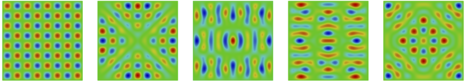
Figure 2. Square: Eigenvectors corresponding to the eigenvalues $128\pi^{2}$ (left) and $130\pi^{2}$.

7.2. L-Shape

(a) Convergence rates for
$\lambda_{1}\approx 9.6397238$.

(b) Convergence rates for
$\lambda_{2}\approx 15.197252$.

(c) Convergence rates for
$\lambda_{3}=2\pi^{2}$.

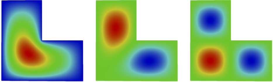
(d) L-Shape: Contour plots of the computed approximations of the first three eigenvectors.

Figure 3. L-Shape: Convergence rates for $\lambda_{1}$, $\lambda_{2}$ and $\lambda_{3}$.

Let $\Omega$ be the $L$-shaped domain that is the concatenation of three unit squares; see Figure 3(d). In [29], the authors provide very precise approximations of several eigenvalues for this domain (and other planar domains). Their approximations of the first three eigenvalues (accurate to eight digits) are

$$\lambda_{1}\approx 9.6397238\quad,\quad\lambda_{2}\approx 15.197252\quad,\quad\lambda_{3}=2\pi^{2}\approx 19.739209~{},$$

and we take the first two of these approximations to be the “truth” for purposes of our convergence studies. We use the search interval $(0,20)$.

These eigenvalues correspond to eigenvectors having very different regularities, and the convergence plots in Figure 3 illustrate that (55) can be pessimistic in the sense that it ascribes a single convergence rate to an entire eigenvalue cluster, and this convergence rate is dictated by the worst-case regularity of eigenvectors associated with the cluster. What we see in practice is that individual eigenvalues within a cluster converge at rates determined by the regularity of their corresponding eigenvectors. Since $\Omega$ has a re-entrant corner with interior angle $3\pi/2$, we have $r=\min(s,p)=s$ for any $s<2/3$, and the first eigenvector actually has this regularity. As such, Theorem 6.3 indicates essentially ${\mathcal{O}}(h^{4/3})$ convergence for the cluster. While this is true for the cluster as a whole, it is only the first eigenvalue that converges this slowly. The convergence order for the second eigenvalue ${\mathcal{O}}(h^{\min(2p,3)})$, is consistent with a regularity index $s\leq 3/2$; and the convergence order for the third eigenvalue, ${\mathcal{O}}(h^{2p})$, is precisely what is expected from an analytic eigenvector.

7.3. Dumbbell

Let $\Omega$ be the dumbbell-shaped domain that is a concatenation of two unit-squares joined by a $1/4\times 1/4$ square “bridge”; see Figure 4. By tiling the dumbbell with $(1/8)\times(1/8)$ squares, we see that $\lambda=128\pi^{2}\approx 1263.309$ is an eigenvalue, with corresponding eigenvector $e=\sin(8\pi x)\sin(8\pi y)$. In order to determine whether there are other eigenvalues near $128\pi^{2}$, we choose the search interval $(1262,1264)$. Because of the highly oscillatory nature of the eigenvector $e$, we employ relatively fine discretizations, taking $p=3$ and $h=2^{-4},2^{-5},2^{-6},2^{-7}$. We have determined that there is one other eigenvalue in the search interval, and it is approximately $1262.41$. Labeling these eigenvalues $\lambda_{1}\leq\lambda_{2}$, their computed approximations are given in Table 1. For the coarsest of these discretizations, the computed approximation of $128\pi^{2}$, $1264.02$, lies slightly outside the search interval, but is accepted by the algorithm. Since $\lambda_{2}=128\pi^{2}$ is known, we underline the number of correct digits in our approximations of it. The error in this approximation is consistent with ${\mathcal{O}}(h^{6})$ eigenvalue error, in agreement with Theorem 6.3.

Table 1. Dumbbell: Computed eigenvalues for the interval $(1262,1264)$, $p=3$ and mesh parameters $h=2^{-4},2^{-5},2^{-6},2^{-7}$.

$h$	$\lambda_{1}$	$\lambda_{2}$
$2^{-4}$	1263.178867	1264.020566
$2^{-5}$	1262.447629	1263.319956
$2^{-6}$	1262.418298	1263.309521
$2^{-7}$	1262.410062	1263.309366

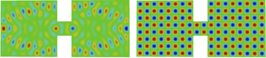
Figure 4. Dumbbell: Eigenvectors corresponding to the eigenvalues $1262.41$ (left) and $128\pi^{2}$.

References

- [1] P. M. Anselone and T. W. Palmer, Spectral analysis of collectively compact, strongly convergent operator sequences, Pacific J. Math., 25 (1968), pp. 423–431.
- [2] A. P. Austin and L. N. Trefethen, Computing eigenvalues of real symmetric matrices with rational filters in real arithmetic, SIAM J. Sci. Comput., 37 (2015), pp. A1365–A1387.
- [3] I. Babuška and J. Osborn, Eigenvalue problems, in Handbook of numerical analysis, Vol. II, Handb. Numer. Anal., II, North-Holland, Amsterdam, 1991, pp. 641–787.
- [4] W.-J. Beyn, An integral method for solving nonlinear eigenvalue problems, Linear Algebra Appl., 436 (2012), pp. 3839–3863.
- [5] T. Bühler and D. A. Salamon, Functional Analysis, vol. 191 of Graduate Studies in Mathematics, American Mathematical Society, Providence, RI, 2018.
- [6] A. Ern and J.-L. Guermond, Theory and practice of finite elements, vol. 159 of Applied Mathematical Sciences, Springer-Verlag, New York, 2004.
- [7] J. Gopalakrishnan, L. Grubišić, and J. Ovall, Iterative convergence of filtered subspace iteration for unbounded selfadjoint operators, In Preparation, (2018).
- [8] J. Gopalakrishnan, L. Grubišić, J. Ovall, and B. Q. Parker, Analysis of the FEAST iteration with DPG discretization, In Preparation, (2018).
- [9] J. Gopalakrishnan and B. Q. Parker, Pythonic FEAST. Software hosted at Bitbucket: https://bitbucket.org/jayggg/pyeigfeast, 2017.
- [10] P. Grisvard, Singularities in boundary value problems, vol. 22 of Recherches en Mathématiques Appliquées [Research in Applied Mathematics], Masson, Paris; Springer-Verlag, Berlin, 1992.
- [11] P. Grisvard, Elliptic problems in nonsmooth domains, vol. 69 of Classics in Applied Mathematics, Society for Industrial and Applied Mathematics (SIAM), Philadelphia, PA, 2011. Reprint of the 1985 original.
- [12] L. Grubišić, V. Kostrykin, K. A. Makarov, and K. Veselić, Representation theorems for indefinite quadratic forms revisited, Mathematika, 59 (2013), pp. 169–189.
- [13] S. Güttel, Rational krylov methods for operator functions, Dissertation Thesis, Bergakademie Freiberg, (2010).
- [14] S. Güttel, E. Polizzi, P. T. P. Tang, and G. Viaud, Zolotarev quadrature rules and load balancing for the FEAST eigensolver, SIAM J. Sci. Comput., 37 (2015), pp. A2100–A2122.
- [15] R. Huang, A. A. Struthers, J. Sun, and R. Zhang, Recursive integral method for transmission eigenvalues, J. Comput. Phys., 327 (2016), pp. 830–840.
- [16] A. Imakura, L. Du, and T. Sakurai, Relationships among contour integral-based methods for solving generalized eigenvalue problems, Jpn. J. Ind. Appl. Math., 33 (2016), pp. 721–750.
- [17] D. S. Jerison and C. E. Kenig, The Neumann problem on Lipschitz domains, Bull. Amer. Math. Soc. (N.S.), 4 (1981), pp. 203–207.
- [18] T. Kato, Perturbation theory for linear operators, Classics in Mathematics, Springer-Verlag, Berlin, 1995. Reprint of the 1980 edition.
- [19] A. Knyazev, A. Jujunashvili, and M. Argentati, Angles between infinite dimensional subspaces with applications to the Rayleigh-Ritz and alternating projectors methods, J. Funct. Anal., 259 (2010), pp. 1323–1345.
- [20] A. V. Knyazev and M. E. Argentati, Rayleigh-Ritz majorization error bounds with applications to FEM, SIAM J. Matrix Anal. Appl., 31 (2009), pp. 1521–1537.
- [21] E. Polizzi, Density-matrix-based algorithms for solving eigenvalue problems, Phys. Rev. B., 79 (2009), p. 115112.
- [22] M. Reed and B. Simon, Methods of modern mathematical physics. I. Functional analysis., Academic Press [Harcourt Brace Jovanovich Publishers], New York, 1972.
- [23] Y. Saad, Analysis of subspace iteration for eigenvalue problems with evolving matrices, SIAM J. Matrix Anal. Appl., 37 (2016), pp. 103–122.
- [24] T. Sakurai and H. Sugiura, A projection method for generalized eigenvalue problems using numerical integration, in Proceedings of the 6th Japan-China Joint Seminar on Numerical Mathematics (Tsukuba, 2002), vol. 159:1, 2003, pp. 119–128.
- [25] A. H. Schatz, An observation concerning Ritz-Galerkin methods with indefinite bilinear forms, Math. Comp., 28 (1974), pp. 959–962.
- [26] K. Schmüdgen, Unbounded self-adjoint operators on Hilbert space, vol. 265 of Graduate Texts in Mathematics, Springer, Dordrecht, 2012.
- [27] J. Schöberl, NGSolve. http://ngsolve.org, 2017.
- [28] P. T. P. Tang and E. Polizzi, FEAST as a subspace iteration eigensolver accelerated by approximate spectral projection, SIAM J. Matrix Anal. Appl., 35 (2014), pp. 354–390.
- [29] L. N. Trefethen and T. Betcke, Computed eigenmodes of planar regions, in Recent advances in differential equations and mathematical physics, vol. 412 of Contemp. Math., Amer. Math. Soc., Providence, RI, 2006, pp. 297–314.