Environmental effects on galaxy evolution. II: quantifying the tidal features in NIR-images of the cluster Abell 85

Abstract

This work is part of a series of papers devoted to investigate the evolution of cluster galaxies during their infall. In the present article we imaged in NIR a selected sample of galaxies throughout the massive cluster Abell 85 (z = 0.055). We obtained (JHK’) photometry for 68 objects, reaching ${\sim}$1 mag arcsec^-2 deeper than 2MASS. We use these images to unveil asymmetries in the outskirts of a sample of bright galaxies and develop a new asymmetry index, ${\alpha}_{An}$, which allows to quantify the degree of disruption by the relative area occupied by the tidal features on the plane of the sky. We measure the asymmetries for a subsample of 41 large area objects finding clear asymmetries in ten galaxies, most of them being in groups and pairs projected at different clustercentric distances, some of them located beyond $R_{500}$. Combining information on the -gas content of blue galaxies and the distribution of sub-structures across Abell 85, with the present NIR asymmetry analysis, we obtain a very powerful tool to confirm that tidal mechanisms are indeed present and are currently affecting a fraction of galaxies in Abell 85. However, when comparing our deep NIR images with UV-blue images of two very disrupted ($jellyfish$) galaxies in this cluster, we discard the presence of tidal interactions down to our detection limit. Our results suggest that ram-pressure stripping is at the origin of such spectacular disruptions. We conclude that across a complex cluster like Abell 85, environment mechanisms, both gravitational and hydrodynamical, are playing an active role in driving galaxy evolution.

1 Introduction

Since several decades, many efforts have been devoted to understand the origin of the density morphology relation (see e.g. Dressler, 1980, and references therein). The fact that in the nearby universe spiral galaxies are systematically less abundant in the central cluster regions, compared with the field, constitutes important evidence that environment has been playing an important role in galaxy evolution at least since $z\sim$ 0.5 (Lewis et al., 2002; Koopmann & Kenney, 2004; Boselli & Gavazzi, 2006; Bamford et al., 2009; Jaffé et al., 2011, 2016). Inversely, this remarkable absence of spirals near the cluster cores is accompanied by a growing population of lenticulars towards high density regions. This raises the question of whether a large fraction of spirals is being transformed into S0’s during their infall towards galaxy clusters (Kodama & Smail, 2001; Erwin et al., 2012; Rawle et al., 2013). Some authors propose that two types of lenticulars could exist, one of them corresponding to the processed spiral galaxies (Bedregal et al., 2006; Barway et al., 2007; Calvi et al., 2012).

There is indisputable evidence for cluster environment effects on individual galaxies, but determining which are the main physical processes driving galaxy evolution is still a matter of debate. Such mechanisms are classified in two types: the hydrodynamic mechanisms exerted by the hot intra cluster medium (ICM) e.g. ram pressure stripping (Gunn & Gott, 1972) and gravitational processes. The latter include both galaxy-galaxy and/or galaxy-cluster interactions (Merritt, 1983; Byrd & Valtonen, 1990; Moore et al., 1996). Presently, it is currently accepted that more than one single mechanism must be at work, specially on the galaxies undergoing strong morphological transformations during their infall onto the cluster (Cortese et al., 2007; Yoshida et al., 2012; Ebeling et al., 2014; McPartland et al., 2016).

While imaging the HI in late-types is a direct tool to study ram-presure stripping (Bravo-Alfaro et al., 2000, 2001; Poggianti & van Gorkom, 2001; Kenney et al., 2004; Crowl et al., 2005; Chung et al., 2007, 2009; Scott et al., 2010, 2012; Jaffé et al., 2016), tracing the tidal features is not always straightforward, observationally speaking. First, such structures show up (most times) at low surface brightness. Second, the old stellar population is a very good tracer of gravitational tidal structures (Plauchu-Frayn & Coziol, 2010) and these stars are better seen in NIR; in this band the contamination produced by star forming regions (at least in the case of spirals) is lower than in the optical bands. Therefore deep NIR imaging is best suited to study tidal disruptions (e.g. WINGS, Valentinuzzi et al., 2009). Traces of old stars (several gigayears old) found along tidal structures constitute the smoking gun of gravitational interactions. Old stars could only be teared up from the galaxy disk by tidal interactions, while young stars could be formed in situ from ram-pressure stripped gas. However, observing in the NIR raises a number of difficulties, starting with the fact that relatively complex techniques are needed to observe and reduce data in the J, H, K bands. Using the available 2MASS images is not an option to tackle this issue when dealing with objects at $z$${\sim}$0.01 (and beyond), because these images are not deep enough to unveil the low surface brightness features (see Sect. 2.3).

To complicate the issue, a direct comparison between different surveys is rarely straightforward, either because the observed samples are different (in morphology, environment or redshift) or because the method to quantify the tidal features are not the same (see e.g. Adams et al., 2012, and references therein). In this respect, Holwerda et al. (2014) reviewed the methods presently available to determine galaxy morphologies and tidal features. They reported several criteria to identify disturbed galaxies, involving parameters like the flux 2nd-order moment (Lotz et al., 2004), the CAS system (Conselice, 2003), and the Gini index (Abraham et al., 2003).

With the aim of quantifying the role played by tidal interactions in the evolution of galaxies in nearby clusters, we develop a new asymmetry index which is well suited to measure low surface brightness asymmetries in the outskirts of galaxies. Our method is applied here to a few dozens of member galaxies of Abell 85 (z = 0.055), a complex system where tidal mechanisms are expected to be significant. This cluster has a large set of observational data, going from X-ray (Ichinohe et al., 2015), VLA-HI data (Bravo-Alfaro, et al. in prep.), to optical imaging and spectroscopy. The studies of the substructures of A 85 (Durret et al., 1998b; Bravo-Alfaro et al., 2009; Yu et al., 2016), provide useful information to correlate with gravitational pre-processing. This paper constitutes a step further in a broader study on galaxy evolution in clusters; our previous work on A 85 (Bravo-Alfaro et al., 2009) tackled the corrrelation between the -content of late-types and their position within different substructures throughout the cluster. The following papers of this series will be devoted to large field coverage of several nearby systems (including A 85, A 496 and A 2670), both in NIR and , in order to study the evolution of galaxies on statistical basis.

The present paper is organized as follows. In Sect. 2 we describe our survey, the NIR-observing strategy, and the flux calibration. We provide a NIR (J,H,K’) catalog for the sampled galaxies. In Sect. 3 we describe our method to measure the asymmetry features. We compare our asymmetry index with other tools currently available in the literature. In Sect. 4 we discuss the fraction of galaxies showing asymmetries and their positions across A 85. We present a global view of the cluster confirming the presence of some physical pairs and groups of galaxies, taking into account the tidal interactions we unveil in the NIR. In Sect. 4.2 we describe the most interesting cases of individual galaxies in selected fields, including three very disrupted objects (two of them being classified as $jellyfish$ galaxies). Sect. 5 provides a summary and our main conclusions.

Throughout this paper we assume $\Omega_{M}$ = 0.3, $\Omega_{\Lambda}$ = 0.7, and H₀ = 75 km s^-1 Mpc^-1. In this cosmology, 10^′  are equivalent to  0.6 Mpc at the distance of Abell 85.

2 Observations and data reduction

2.1 The sample

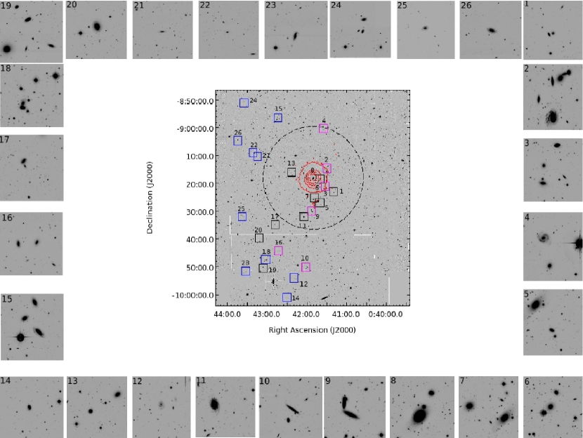
Figure 1: Central panel: optical (CFHTg) image of the cluster Abell 85, showing the positions and the size of the 26 fields observed in this work. The white square (Field 8) indicates the position of the cD galaxy. Blue squares correspond to fields having blue -rich objects. Magenta squares show the location of fields with asymmetric galaxies. The red contours trace the X-ray emission (XMM-Newton (Ichinohe et al., 2015)), and the dotted circle draws the physical radius R₅₀₀ (${\sim}$1.2 Mpc). A zoom of each field is displayed around the central panel; the field number is on the top-left.

Fig. 1 shows the location of the 26 fields observed throughout A 85. These fields were chosen under several criteria (see Column 7 of Table 1). First, we targeted the ten -detections (excluding two marginal ones) reported by Bravo-Alfaro et al. (2009) (hereafter BA09). This is with the aim of studying their evolutionary stage while moving towards/across the cluster. Second, after visual inspection, we selected the fields displaying (at least in projection) pairs or groups of bright galaxies. These are places where we expect to see tidal features at different degrees. Another field was devoted to the cD, A85[DFL98]242, and one more to a galaxy showing some asymmetries (A85[DFL98]276), but being apparently isolated (under projection and velocity criteria), see Table 1.

Our selected fields include the brightest galaxies in A 85. With a few exceptions, all these objects are members of A 85, following the membership (position-velocity) criteria given by BA09. The observed sample is complete up to $B_{J}=16$ (following the SuperCOSMOS database), for the redshift range of the cluster and within a region going from 00h 40m 30s to 00h 44m 00s in R.A., and from -08^∘ 45^′  00^′′  to -10^∘  05^′  00^′′  in declination. This sample is devoted to obtain a first insight on the presence of tidally disrupted galaxies in A 85, and to quantify their degree of asymmetry. In total, we obtained NIR magnitudes for 68 galaxies, projected inside a radius of 1^∘  from the cluster center, which we take as coincident with the position of the cD galaxy. Table 2 gives the optical parameters of the observed objects.

2.2 Image acquisition and processing

We selected 26 fields in the A 85 galaxy cluster to be observed in the NIR bands JHK’ (1.28, 1.67, 2.12 $\mu$m). The K’ filter is available at the OAN instead of the K-band one; their effective wavelengths are the same, i.e. $2.12\mu$m. All our images were obtained between 2006 and 2011 at the 2.1m telescope of the National Astronomical Observatory (OAN), in San Pedro Martir, Mexico. We used the NIR camera CAMILA (Cruz-González et al., 1994), equipped with a 256$\times$256 pixels NICMOS3 detector array. The image scale is 0.85^′′ pixel^-1, and the field of view is 3.6^′$\times$3.6^′. Some optical vignetting reduced the useful fov to 3.0^′. The seeing during our observing runs varied between 2.0^′′and 2.5^′′.

Due to the high sky brightness and variability, seen in the NIR, we chose a “telescope chop” strategy, in order to properly scan the sky background in every band. Typically, our galaxies do not extend over a large fraction of the detector, most of them having a major axis well below one arcminute. So instead of the ”on/off target” strategy, we offset the pointing-center by less than one arcminute between exposures. With this technique we manage to keep the targets on different zones of the CCD, distributed along the four detector quadrants, thus saving observing time.

The linearity range of the detector constrained us to apply short individual sub-exposures in order to avoid saturation. These limits are typically 30s, 20s, 5s, for J, H and K’, respectively. We made sequences of 9 pointings of 60s each, splitting the 60s, in order to avoid saturation, into 2x30s, 3x20s and 12x5s, depending on the waveband. We applied the mentioned offsets between pointings, and we repeated the sequences until reaching total integration times in the range 1600s-3800s (see Table 1). With this strategy, the median average of the nine frames provides a good sky image, where the cosmic rays, the stars and the galaxies themselves, have been removed.

The image processing and calibration were performed using IRAF. We followed standard procedures for data reduction, following Barway et al. (2005) and Romano et al. (2008). For the flat-fielding we applied the twilight sky method and obtained two different sets of images, those with high count levels (“bright flats”) and those with low count levels (“dark flats”). We combined the dark and bright flats separately, and then subtracted the dark flat from the bright one. The resulting frame was normalized by its mean value, and this master flat was used for general flat fielding. This procedure was repeated for each observed band.

A key step is the sky subtraction. We combined all the frames, within a nine-image sequence (see above), by using the median criteria. The resultant frame constitutes a good sky image, which is subtracted from each individual image of the corresponding sequence. The resulting sky-free images were aligned to a common coordinate system by using stars appearing in all frames. Finally, these images were averaged, delivering a final, cleaned image for each band. All the procedure described above was carried out by applying the script $CAMILA$, developed by one of us (YDM). As a last step, we carried out the corresponding astrometry, by matching the galaxy coordinates using the 2MASS catalog from the NASA/IPAC Infrared Science Archive (IRSA).

2.3 Flux calibration and photometry

We observed a set of photometric standard stars in order to carry out the flux calibration. Here, the strategy for image reduction followed the procedure described in Sect. 2.2. The only difference was the application of shorter integration times (a few seconds) for the standard stars, as their magnitudes are much brighter than those of our science targets. The observed standards (FS 101, FS 104, FS110, FS111, FS112, FS119, FS150, FS154) were selected from the Persson et al. (1998) and Hawarden et al. (2001) catalogs. We observed several standards during each night, under different airmasses, in order to improve the accuracy of our zero-points (ZP). We solved the following equation to calculate the ZPs in each band:

$$m_{\lambda}=-2.5logR_{\lambda}+ZP_{\lambda}$$ (1)

where $R_{\lambda}$ represents the instrumental counts and $ZP_{\lambda}$ is the zero-point constant, in each filter. NIR zero-points are found to be stable, not only during a single night, but over several nights through the whole observing run. For each night we have estimated the known magnitude of one standard star, by using the ZP of other standards observed along the same night. The magnitudes obtained this way, matched very well with each other. In the end we average the individual $ZP$ coming from different stars, ensuring that the ZP value is correct.

We obtained aperture magnitudes (14^′′  in diameter) for galaxies in our sample as this allows direct comparison with published NIR catalogs. We measured these magnitudes with SExtractor (Bertin & Arnouts, 1996). We first ran SExtractor in single-image mode for the J-band, which has the highest S/N ratio. We then ran SExtractor again in dual mode, with the J-band frame as the reference, and we computed the magnitudes of H and K’ bands. This procedure ensured that the measurements of each galaxy, in all three filters, were done exactly over the same pixels. In the end, from the 71 objects targeted in Table 2. we obtained good quality images and magnitudes for 68 galaxies (see Table 3). Three of the objects previously detected in HI ([SDL98]3114, and [DFL98]323/461, see BA09) are faint objects and have very blue colors, therefore, our NIR images did not provide enough signal to obtain accurate magnitudes. These objects are not included in our further analysis.

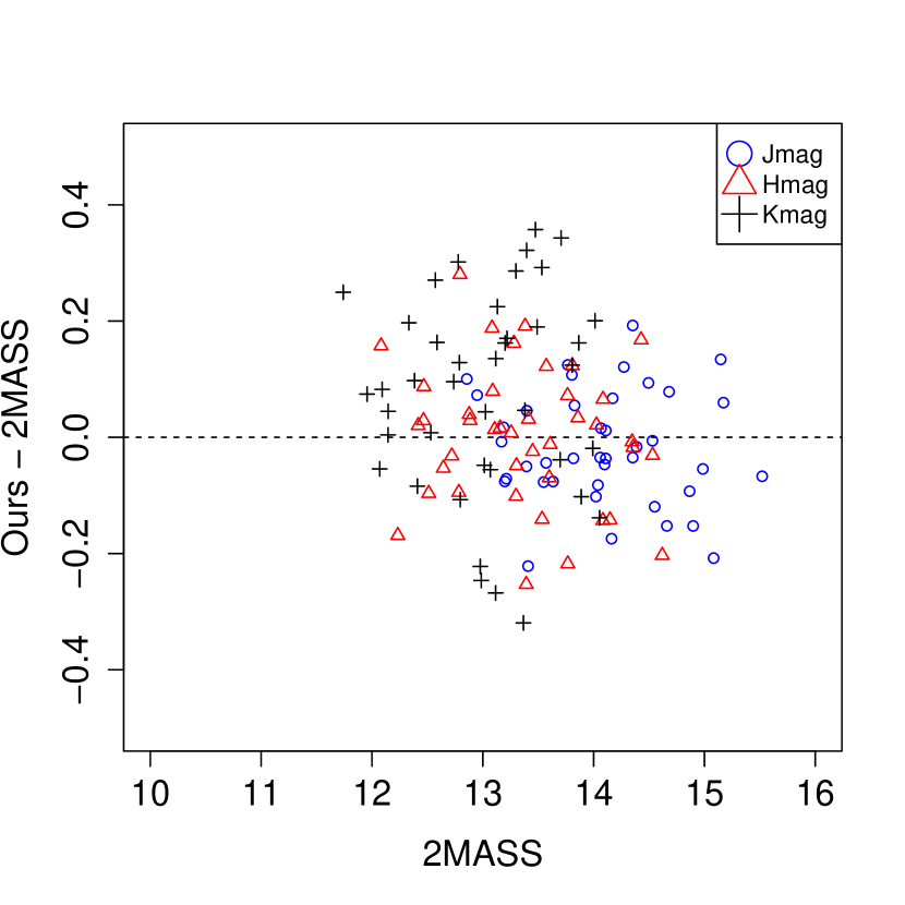
Figure 2: Comparison of 2MASS magnitudes with the NIR values obtained in this work ($Ours$). The X-axis displays 2MASS magnitudes and the Y-axis indicates the difference $Ours-2MASS$. A slight trend is observed on our K’ magnitudes being -in average- larger than 2MASS’. This is not shown by the other two bands (see text).

Forty-one galaxies of the 68 in our photometric sample have NIR magnitudes in the 2MASS catalog. We compared our 14^′′  aperture magnitudes, shown in Table 3, with those published by 2MASS. This allows to test the quality of our imaging procedure and the accuracy of our photometric data. We have found a good match between both catalogs (see Fig. 2). As expected, we obtained a slightly larger deviation in the K’-band, as the noise is higher at this frequency. Our magnitudes in this band display a slight trend being, in average, larger than 2MASS. The most likely explanation is linked to the (rather long) age of the NIR camera at the time of our observing runs; the detector and/or other optical parts of the instrument could lose sensitivity after decades of service. If so, this could affect in first term the K’ band, rather than J, H, where the effect is not seen (Fig. 2). Nevertheless, this bias is not significant: the average differences between our magnitudes and those from 2MASS (in absolute values), and corresponding standard deviations, are 0.08$\pm$0.05 for J, 0.10$\pm$0.08 in H, and 0.16$\pm$0.10 in K’. The first advantage of our survey, compared with 2MASS (within the observed area), is the higher number of galaxies with reported magnitudes. And second, our frames are deeper by (roughly) one magnitude arcsec^-2 when compared with 2MASS. Our survey reached, on average, the following 1-sigma background noise and corresponding errors: 22.40$\pm$0.06, 21.20$\pm$0.07, and 20.30$\pm$0.06 mag arcsec^-2, in J, H, and K’, respectively. The corresponding 2MASS values are 21.4, 20.6, and 20.0 (Jarrett et al., 2003).

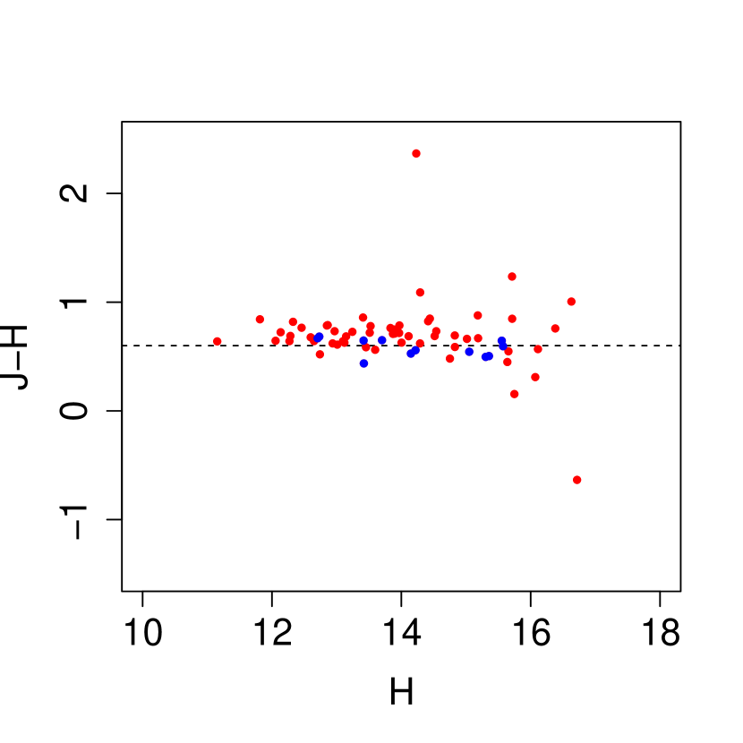
Figure 3: Color-magnitude plot (J-H) vs H of isophotal magnitudes of the 68 galaxies observed in this work. Blue dots correspond to blue galaxies, as reported by BA09. The red dots indicate early-type galaxies. The dotted line at (J-H) = 0.6 is a reference for the red sequence for NIR data.

In order to illustrate the photometric properties of our sample we display a color-magnitude diagram (J-H) vs J (Fig. 3), based on our total isophotal magnitudes. These values were obtained with SExtractor, with a detection threshold of 1$\sigma$ measured on the background. We plot, as a reference, a red sequence (at J-H = 0.6) derived using 2MASS data (Caretta 2015, priv. comm.) This figure shows that our sample is rather dominated by red objects. Two galaxies appear with extreme colors in this plot, and should be taken with caution. One of them is displaying an abnormal red color (A85[SDG98]1951), probably because of contamination of the neighbor cD halo (see Sect. 4.2). Another galaxy (A85[SDG98]2260), appears with an extremely blue color (bottom-right corner of Fig. 3); this object is lying on the very edge of the corresponding field, which could have affected its photometry.

3 Measuring the asymmetry features

3.1 The asymmetry index ${\alpha}_{An}$

The main goal of this work is to detect and quantify asymmetry features in galaxies produced through tidal interactions. With this aim we apply an asymmetry analysis which is focused on the old stellar morphology drawn by NIR images. Measuring asymmetries has proven to be useful with images at different wavelengths, including optical and . This work is intended to be a first approach to measure the role played by gravitational mechanisms in the evolution of galaxies in A 85, within its middle and high density regions.

Visual inspection remains as one of the best suited techniques to classify galaxies (McIntosh et al., 2004; Mihos et al., 2005). However, considering the huge amount of data available nowadays, this method is very limited. Furthermore, visual classification does not provide quantitative information, for instance, about the degree of disruption a galaxy is undergoing, thus reducing the possibility of any statistical study. This raises the importance of methods that quantify the morphological properties of galaxies, as they allow to correlate those properties with environment conditions and, in the end, to shed light on the physics driving galaxy evolution.

Our strategy to measure galaxy asymmetries was the following. First, we select within our sample those galaxies having angular dimensions above a certain threshold in order to keep only those objects with enough data points. This subsample consists of the 41 galaxies having major axis $a\geqq 15$^′′  (or ${\sim}$18 pixels), and minor axis $b\geqq 7.5$^′′, (${\sim}$9 pixels). As our uncertainty is dominated by the seeing (i.e. 2.5^′′  or 3 pixels), our criteria implies that we keep a maximum linear uncertainty of 16%  on $a$, and 30%  on $b$. Propagating these errors when calculating the area of the galaxies, we keep an uncertainty below the threshold $\leq$33%.

Next, for the 41 selected galaxies we generate a 2-D intensity map by applying the IRAF task ELLIPSE (STSDAS package). We apply this technique only to J-band images, as they have a more homogeneous background and higher S/N ratio than the H and K’ frames. The ELLIPSE routine, described by Jedrzejewski (1987), calculates the Fourier series:

$$I(\phi)=I_{0}+\Sigma\ a_{n}\ sin\ (n\phi)+\Sigma\ b_{n}\ cos\ (n\phi)$$ (2)

where $\phi$ is the ellipse eccentric anomaly, $I_{0}$ is the mean intensity along the ellipse, and $a_{n}$, $b_{n}$ are harmonic amplitudes, along the major and minor axis, respectively. Typically we start the fit at 2.5^′′  from the center of the galaxy, which avoids the bulge (for spirals) and minimizes the effects produced by the seeing (see Sect. 2.2). This fitting provides the mean radial light distribution and the variation of the three parameters: center ($x_{o},y_{o}$), ellipticity ($E$), and position angle ($p.a.$), as a function of the galaxy radius. We stop the fitting when reaching isophotes having counts equal to three times the standard deviation of the background ($3\sigma_{bg}$), equivalent to a surface brightness of 21.2 mag arcsec^-2, in average. For most of our galaxies, this occurs at a radius of ${\sim}$12 pixels, equivalent to a linear radius of 10 kpc from the galaxy center.

We run a second iteration of ELLIPSE; this time we fix the three parameters (center, $E$, $p.a.$) to values obtained around 6-7 kpc from the galaxy center, with the aim of avoiding the outskirts. In this fashion we get a final intensity profile which is used as input of the IRAF task BMODEL. This task will produce a 2D axy-symmetric model of the galaxy, in a frame where the background is defined as zero. Hereafter, this symmetric ”clone” of the galaxy, will be named the $bmodel$, which is subtracted from the original object, delivering a residual image. The original image and the residual one will be named the $observed$ and the $residual$ images, respectively. During this procedure, the central pixels of the galaxy are actually not considered in our analysis, as we are rather interested in the galaxy outskirts, where we expect less bound material to be more easily distorted when tidal effects are exerted on the galaxy.

Based on the residual described above, we define a new asymmetry index, named ${\alpha}_{An}$  ($A$ for ”area”; and $n$ makes reference to the threshold applied above the background level). In simple terms, our index is described by the following expression:

$${\alpha}_{An}=N_{res}(>n*\sigma)~{}/~{}N_{tot}(>n*\sigma)$$ (3)

where $N_{res}(>n*\sigma)$ is the number of pixels measured upon the residual image having counts above the limit $n*\sigma$. $N_{tot}(>n*\sigma)$ is the number of pixels of the parent galaxy registering counts above the same cutoff. We stress that this limit is the same standard deviation of the background ($\sigma_{bg}$) described in the previous paragraphs. We keep $\sigma$ in our equations in order to make the notation simpler.

This tool is defined to deliver complementary information to that provided, for instance, by the CAS asymmetry index and by other tools, like the Gini equality parameter. Our index is devoted to measure how prominent (in surface) are the asymmetry features in a galaxy, compared with the galaxy itself. In other words, ${\alpha}_{An}$  gives the relative $area$ of the features, normalized to their parent galaxy. The physical information provided by the area of asymmetry features is complementary to the information provided by tools measuring the intensity. Actually, the ${\alpha}_{An}$  index is intended to resolve the ambiguity between two galaxies having the same $A$ (CAS) index, where one of them has low surface brightness tidal tails, spread on a large area, from another galaxy with small bright features. Distinguishing between the two cases has important physical implications, like applying constraints to the age of the event being at the origin of the interaction; this could be done by comparing the observed asymmetry features with current models of tidal interactions. From the two cases drawn above, the first event (with more spread features) would be expected to be older than the second one, with small and bright asymmetries, more embedded in the inner regions of the parent galaxy.

The index ${\alpha}_{An}$  is obtained by measuring the surface of the asymmetry features, in pixels, upon the residual image obtained after the subtraction: $observed-bmodel$. We apply a cutoff in order to define the borders of the asymmetry features and to ensure that our index is only taking into account the pixels that are brighter than our defined threshold.

As a second step, we estimate the total area covered by the parent galaxy, which is measured on the $bmodel$ image. Here, we apply the same criteria that we used to measure the asymmetry features, i.e. we consider only those pixels above the defined surface brightness limit, in order to obtain the total number of pixels covered by the galaxy. Obtaining the galaxy size upon the $bmodel$ image, instead of the original one, makes the galaxy measurement more homogeneous. We finally divide the number of pixels of the asymmetry features by the corresponding number of pixels of the parent galaxy. Therefore, ${\alpha}_{An}$  represents the fractional surface of the asymmetry features relative to their parent galaxy (represented by the $bmodel$).

Throughout this work we apply a $3\sigma$ cut while estimating the asymmetries, so hereafter we will often use the more specific notation, ${\alpha}_{A3}$, for the index. In practice we applied the following generalized equation to estimate the ${\alpha}_{An}$  index:

${\alpha}_{An}=[N_{res}(n_{lo}*\sigma)<I<(n_{hi}*\sigma)]~{}~{}/$

$$[N_{tot}(n_{lo}*\sigma)<I<(n_{hi}*\sigma)]$$ (4)

where $I$ is the pixel intensity; $(n_{lo}*\sigma)$ represents the lower limit mentionned in the previous paragraphs, and $(n_{hi}*\sigma)$ is an upper clipping applied in order to discard a few bright (spurious) spikes remaining at the galaxy center on the residual images.

3.2 Error sources

Fist of all, in the process of building the $bmodel$, we are using an elliptical aperture which includes the full galaxy and a large fraction of the sky background. In a few cases, a number of objects (stars and/or galaxies) can be included within that aperture. When such objects are too close to the studied galaxy we applied a mask procedure before obtaining the $bmodel$. The value assigned to the pixels inside the patch is the same than the average background sky. In this fashion we avoid any effect on the asymmetry index that could be produced by nearby projected objects.

Other than the problem of having objects too close to the galaxy under analysis, a number of additional errors might affect the asymmetry measurements, as reported by several authors (Conselice, 2014, and references therein); the most important are: (a) the correct identification of asymmetries and of the pixels occupied by these features; (b) the separation of the background from $signal$ pixels (i.e. those belonging to the main galaxy body $and$ those along the asymmetry features); and (c) the determination of the central pixel of the galaxy.

We deal with the first source of error by obtaining an axial symmetric model of the galaxy (the $bmodel$) as described in the previous section; the residual image unveils the asymmetry features. The second source of error, the proper discrimination of background, was solved by applying a reasonable intensity threshold to the selected pixels. This was applied to both sets of pixels, i.e. those coming from the asymmetries (on the residual image), and those considered as part of the galaxy (on the $bmodel$ frame). We applied everywhere $3\sigma_{bg}$, but in the case when features appear with low surface brightness, the clipping value could be adjusted, for instance, to $2.5\sigma_{bg}$.

Concerning the third source of error, the uncertainty on the determination of the central galaxy pixel, we confirm, as other authors (e.g. Holwerda et al., 2014), that this constitutes a major source of error. In order to estimate the effect that this uncertainty exerts on the index ${\alpha}_{A3}$ , we collected the several central pixel values delivered by the task ELLIPSE (see Sect. 3.1), within a box of 3^′′  around the central intensity peak. This 3^′′-box coincides with the maximum seeing-value affecting our observations. We computed the index ${\alpha}_{A3}$  taking into account each one of these center pixels; in the end we defined the very central coordinates of each galaxy as those producing the minimum asymmetry index. Finally, we measured the dispersion of the ${\alpha}_{A3}$  values obtained in this fashion, as a good indicator of the global error. From the sample of 41 galaxies we obtained a standard deviation of 0.006. Therefore, we settled an uncertainty of 0.01 in ${\alpha}_{A3}$  as a realistic (yet conservative) error value for our asymmetry index.

3.3 Comparing ${\alpha}_{A3}$  with other methods

As mentioned before, several tools have been proposed to quantify asymmetry features by using strategies similar to ours (Holwerda et al., 2014, and references therein). Our index can take values starting from zero, which would correspond to a perfectly symmetric galaxy. Otherwise, ${\alpha}_{A3}$  takes positive values: the higher the index, the larger the asymmetry features compared with the parent galaxy. For instance, ${\alpha}_{A3}$ = 1.0 would represent the case of asymmetry features with a total surface matching the area covered by the parent galaxy. We find systematically ${\alpha}_{A3}$ $<$ 1.0, even for disrupted objects; after applying this index to our sub-sample of 41 galaxies (see Table 4) we obtained values in the range, 0 $<$ ${\alpha}_{A3}$ $\leq$ 0.32. After a detailed inspection of galaxies in our sample we found that a value of ${\alpha}_{A3}$ = 0.10 clearly separates symmetric from asymmetric objects. This value corresponds to features spanning 10% of the area of the parent galaxy.

In principle, the method to unveil asymmetries based on the subtraction of an axi-symmetric model is better suited to analyze early-type galaxies. Nevertheless, if the resolution is high enough, this method has shown to successfully trace internal structures in spirals (see e.g. Mayya et al., 2005), such as bars and rings, that could increase the ${\alpha}_{A3}$ index independently of showing (or not) external tidal features. In such cases we should apply a simple additional step in order to separate internal and external asymmetries. In this work, given the angular size of our galaxies and the data we have, there was no need of applying this last step.

We carried out some comparisons with other techniques of measuring galaxy asymmetries, in order to test the performance and degree of confidence of our index. We briefly describe these comparisons.

3.3.1 ${\alpha}_{A3}$  vs visual classification

A first test devoted to explore the performance of our asymmetry index is the following. We took into account a subsample of galaxies from Nair & Abraham (2010). These authors carried out a visual morphology classification for a large sample of galaxies in the range 0.01$<\,z<\,0.1$. They proposed a discrete, qualitative index ($dist$, increasing with the degree and the number of different asymmetries), going from fully symmetric up to bridged objects. We took twenty galaxies from their sample, all being in the redshift range of Abell 85 ($z$${\sim}$0.05), which span the whole scale of distortions. We applied the ${\alpha}_{A3}$  index to those objects upon the same g-band (SDSS-DR4) images used by Nair & Abraham (2010). By comparing these authors’ index (see Fig. 4) with ${\alpha}_{A3}$, we observed that the later is able to properly separate the disrupted objects from the symmetric ones: every galaxy reported by Nair & Abraham (2010) as being unperturbed, displays values of ${\alpha}_{A3}$  very close to zero. In this plot, objects being reported with important disruptions by Nair & Abraham (2010), would get values above 2.0. Fig. 4 shows a good trend between the two indices up to the domain of large asymmetries. Considering the complex way these authors used to define their index (which, for the twenty selected galaxies, takes values between 1 and above 2500) we applied a natural logarithmic scale to their original values, so we get a clearer plot.

3.3.2 Bmodel vs 180^∘  rotation

Another test to our strategy consisted in applying a different method to unveil asymmetries. For example, the asymmetry index $A$, within the CAS system (Conselice, 2003), measures the asymmetry upon a residual image which is obtained after rotating a galaxy by 180^∘, then subtracting this rotated frame from the original image. The index $A$ is based on the integration of the intensities displayed by those pixels within the residual features.

We applied the 180^∘  rotation method to obtain the corresponding residual image, and we calculated the ${\alpha}_{A3}$  index for the sample of 41 galaxies listed in Table 4. We observed a trend where the $bmodel$ residuals produce higher values of ${\alpha}_{A3}$  than those coming from the 180^∘rotation, suggesting that the first method is slightly better to unveil outskirt features. Considering this result, we favor the $bmodel$ strategy over the 180^∘ rotation. There are additional reasons to favor the former method; first, the residual delivered after the 180^∘rotation is very sensitive to the variations of the galaxy central pixel, and additional steps are needed to minimize this source of error (Conselice, 2014). Second, the 180^∘rotation method is more sensitive to flocculent and to not-very-regular spirals; these properties are expected to increase the asymmetry index independently of any external disruption (Holwerda et al., 2014). Last, but not least, the noise in the residual image, after rotation, becomes very inhomogeneous, complicating the application of any cutoff to compute our asymmetry index. In this respect, the advantage of the $bmodel$-subtraction is that the background of the residual image remains exactly the same than in the original image, because the background is defined as zero in the $bmodel$ image. We leave for our forthcoming paper, a direct comparison between our index and the $A$ index of the CAS system, as it is more convenient to carry out such comparison upon a larger sample of galaxies.

4 Results and discussion

Our asymmetry index, applied in combination with other ones being available in the literature, could provide important information to restrict the age of tidal interactions at the origin of the observed disruptions. For this, we must compare the observed galaxies with tidal interaction simulations, taking into account the time-scales delivered by such models (e.g. Lotz et al., 2004). If we only consider asymmetries along the outskirts of the galaxies, we would expect to find a general trend where recent tidal interactions are drawn by stars being projected closer to their parent galaxy and covering smaller areas than older events. Tidal interactions, with time, tend to show stars spreading through larger regions, making the whole asymmetry features weaken in surface brightness (the projected density of stars will drop as they span through a larger volume). In the case a spiral galaxy is affected by a tidal encounter, we expect a color gradient to appear; a recent event will be dominated by blue light (blue stars are brighter than red ones) and, as time goes on, the asymmetry features will become dominated by red light (as red stars last much longer than blue ones) unless star formation occurs in situ along the gas tails. As a matter of fact, a spiral being recently disrupted (not necessarily by tidal interaction) should appear much brighter in the UV and blue bands than in the NIR ones. We discuss some cases following this trend in Sect. 4.2, and we will explore this dating strategy in a forthcoming paper, based on a larger number of objects.

4.1 The loci of disturbed galaxies in A 85

As expected, combining galaxy positions, radial velocities, substructure analysis, and a measurement of asymmetries in NIR, constitutes a powerful tool to obtain reliable information on the physical mechanisms affecting cluster galaxies. Furthermore, this strategy allows to confirm (or discard) physical pairs and groups, and gives some hints on the degree of interaction for those physical pairs/groups. Considering the sample of 41 galaxies going through our asymmetry analysis, only 10 of them display a significant degree of disruption (i.e. those having 0.10$<$${\alpha}_{A3}$, see Sect. 3.3.1 and Fig. 4). These asymmetries go from mild (${\alpha}_{A3}$${\sim}$0.11) to strong (0.14$\leq$${\alpha}_{A3}$$\leq$0.32). Fig. 5 shows the distribution of asymmetry index values of our sub-sample, illustrating that only a fraction (${\sim}$25%) appears with significant perturbations. We stress that our sample is coming from selected fields in Abell 85, so this fraction of disturbed objects can be biased. We will be tackling this issue, on statistical basis, in our forthcoming papers.

The galaxies with strong asymmetries in the present work are found within six of the 26 observed fields. These fields are distributed across A 85 as follows; two of them (Fields No. 2 and 3, see Fig. 1) were pointed on possible groups of galaxies, showing more than three objects fitting within a small sky region ($\leq$ 2.5^′  equivalent to 150 kpc). As seen in Fig. 1, Fields 2 and 3, are projected onto the cluster core. Three other regions with asymmetric galaxies (Fields 4, 9 and 16) contain pairs/triplets; the first of these fields is 20^′  (1.2 Mpc) north from the cluster center; Field 9 is projected onto the South Blob, ${\sim}$0.75 Mpc south of the cluster center, still within the X-ray ICM emission (Fig. 1); Field 16 is nearly 30^′  (${\sim}$1.8 Mpc) within the SE sub-cluster reported by BA09. Finally, Field 10 is placed at the south outskirts of A 85 (30^′  or 1.8 Mpc), where a disrupted galaxy appears (intriguingly) isolated. In the next section we give further details concerning these galaxies as well as a couple of other striking objects observed in this work.

4.2 Comments on selected fields

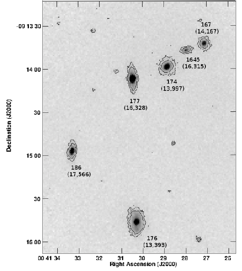
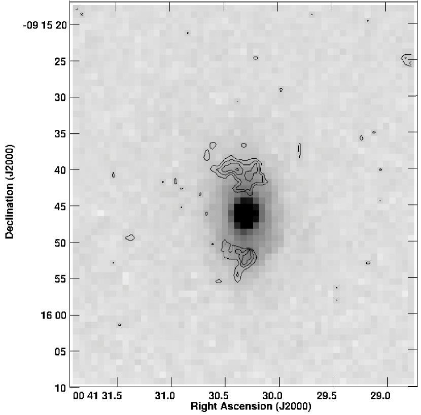
Figure 6: Field 2: A $group$ of galaxies and the $jellyfish$ A85[DFL98]176. Left panel: J-band in contours and grey scale. The first contour corresponds to 3.5 times the $rms$ background level. The names of the galaxies are given following Table 2, and velocities (in  km s^-1) are given in parentheses. Right panel: close up of the $jellyfish$ galaxy A85[DFL98]176 (KAZ 364). The residual image is shown in white contours, overlaid on the J-band image. These contours trace slight asymmetries along the northern and southern edges of the disk. Compare with the UV and blue images in Fig. 7.

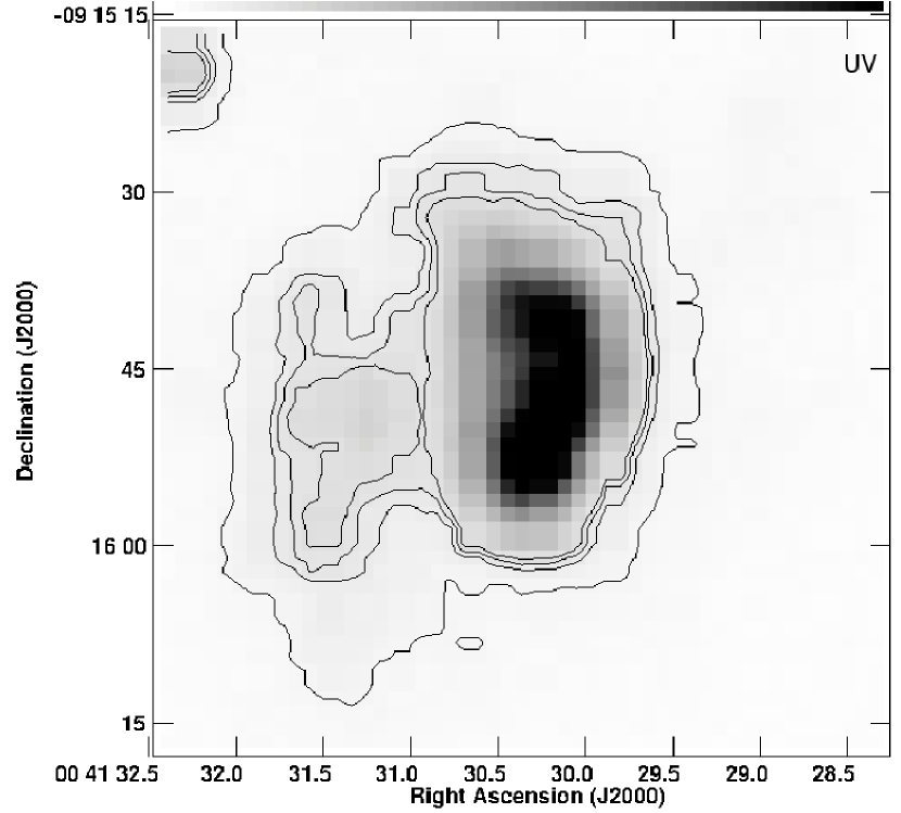
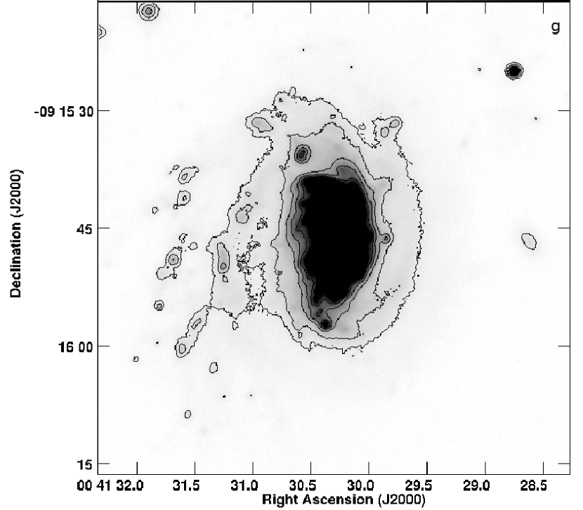
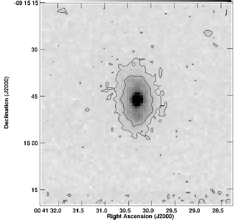
Figure 7: The $jellyfish$ galaxy A85[DFL98]176 (KAZ 364) seen in near-UV (GALEX, top left), optical (MEGACam-g, top right) and J-band (bottom) images. In spite of a slight asymmetry seen in NIR (Fig. 6), this image is not tracing the disrupted arms extending to the SE, clearly seen in blue light.

Field 2, a group around the jellyfish galaxy KAZ 364 This is one of the most exciting regions of our survey. Six bright galaxies are projected within the 3^′$\times$3^′  fov (see Fig. 6): A85[DFL98]176/186/177/174/167 and A85[SDF98]1645. These objects are projected onto a substructure named C2 (see BA09), lying ${\sim}$8^′  (some 0.5 Mpc) NW of the cluster center. One of these galaxies, A85[DFL98]176 (better known as KAZ 364 and JO201, Bellhouse et al. (2017)) is a giant spiral, one of the brightest objects (in the optical bands) in the whole cluster. This object has a velocity lower by ${\sim}$3,000  km s^-1  than the cluster systemic velocity. Seen in blue light, this galaxy shows the pattern known as $jellyfish$, because of the filaments of debris. This object, with its spectacular arm disruption towards the east side, is included in the $jellyfish$ sample of Poggianti et al. (2016). Moreover, when this galaxy is seen in UV-GALEX images, clear emission is seen along the disrupted arms (Fig. 7), but the next pannels of the same figure show that the blue-distorted arms disappear when the galaxy is seen in the NIR. The fact that the asymmetric arms are devoid of old red stars strongly suggests that a very strong RPS event could be at the origin of the stripped pattern. The projected distance from the cluster center (${\sim}$0.5 Mpc) is well within the zone where RPS is expected to have strong effect on gas rich galaxies (BA09).

In addition to the disrupted arms discussed so far, on the east of KAZ 364 and seen only in blue light, other minor asymmetries (${\alpha}_{A3}$  = 0.14) are unveiled by the NIR at the N and S-outskirts of the stellar disk (see Fig. 6). These features do not seem to be linked with the disrupted eastern arms. No obvious neighbor could be blamed for a hypothetical tidal interaction: the two closest objects in projection, A85[DFL98]177/186 do not display strong asymmetries (0.11 and 0.07, respectively), and they have large radial velocities (${\sim}$16,328 and ${\sim}$17,566  km s^-1) relative to KAZ 364 (13,393  km s^-1). Two other objects in the same field, A85[DFL98]167/174, are closer to KAZ 364 in radial velocity (14,167 and 13,997  km s^-1, respectively), and they are projected around 2^′  (120 kpc), N of KAZ 364. In principle, a flyby interaction of KAZ364 with one of the galaxies seen in this field cannot be totally discarded. We conclude that both mechanisms, RPS and a minor tidal interaction, are affecting this galaxy, producing different kinds of asymmetries.

Considering all the galaxies projected within this group, they seem to be part of the loose group $C2$, where no strong tidal interactions seem to occur among the member galaxies, probably because of their high relative velocities. The slight asymmetries we observe could be due to gravitational interactions with the group and/or with the cluster potential.

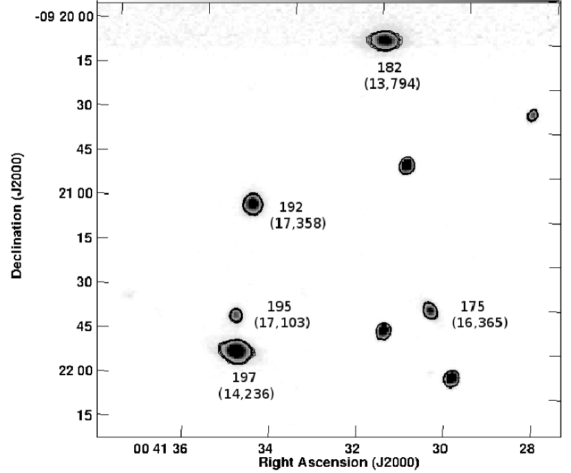
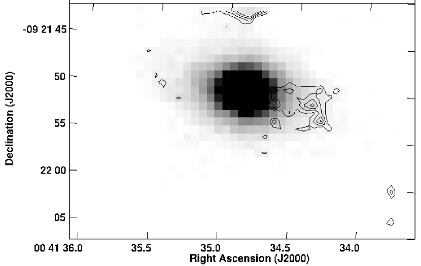
Figure 8: Field 3: a $group$ of galaxies around A85[DFL98]197. Left panel: J-band in contours and grey scale. The first contour corresponds to 3.5 times the $rms$ background level. The names of the galaxies are given according to Table 2. Velocities (in  km s^-1) are indicated in parentheses. Right panel: close up of the galaxy A85[DFL98]197. The residual image, in contours, shows the asymmetries, overlaid on the J-band image (in grey scale).

Field 3, a group around A85[DFL98]197: This region is somehow similar to the previous field; five bright galaxies are projected close to each other, within a region of 2^′  (120 kpc). The brightest object, A85[DFL98]197, displays important NIR asymmetries (${\alpha}_{A3}$= 0.25), strongly suggesting that this galaxy suffered a gravitational interaction (see Fig. 8). Two objects can be responsible for this. The first, A85[DFL98]195, is projected very close (only 0.2^′, or 12 kpc), north of A85[DFL98]197, but they span a large relative velocity of ${\sim}$3,000  km s^-1. On the other hand, A85[DFL98]182 is projected farther to the north (${\sim}$2.0^′, 120 kpc), having a small difference in radial velocities (${\sim}$400  km s^-1). So, a flyby interaction, some 10⁸ yrs ago, between A85[DFL98]197 and A85[DFL98]182, could be at the origin of the observed asymmetry. This timescale is calculated assuming the lower limit for the distance (i.e. the projected distance between the two galaxies), and the velocity dispersion of A 85 (roughly 1,000  km s^-1) as a likely speed difference between the galaxies.

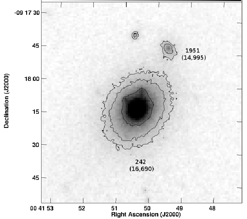
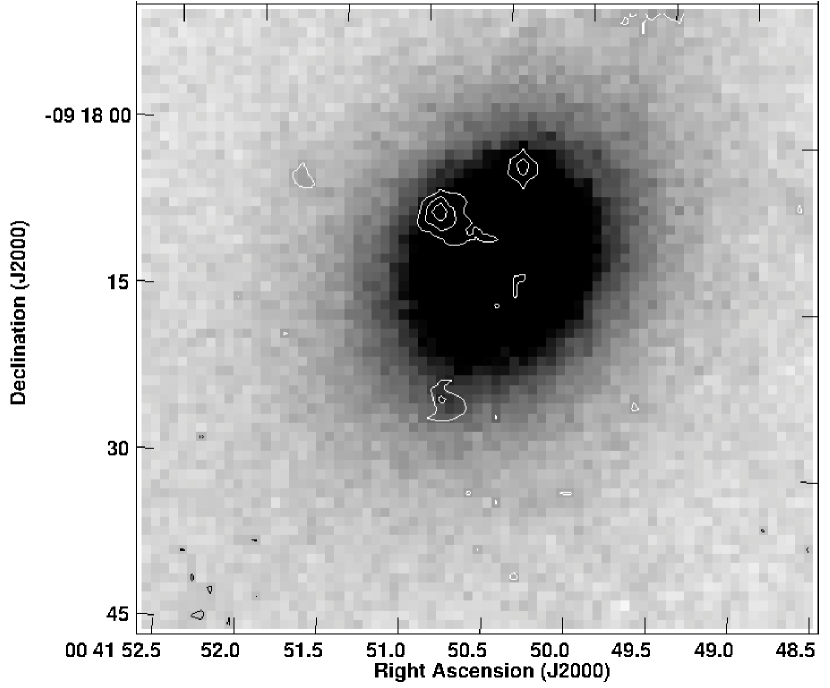
Figure 9: Field 8: The cD galaxy [DFL98]242 and its satellites. Left panel: J-band in contours and grey scale. The first contour corresponds to 3.5 times the $rms$ background level. The names of the galaxies are given according to Table 2. Velocities (in  km s^-1) are given in parentheses. The low mass spiral [SDG98]1951, shows a degree of asymmetry through direct visual inspection. Right panel: The residual image of the cD galaxy is shown in contours, overlaid on the J-band image. This unveils three objects which are suspected to be deep in the cD halo. No redshifts are available for these low-mass galaxies.

Field 8, the cD galaxy A85[DFL98]242: This field, at the very center of A 85, shows some interesting results. While the cD appears globally unperturbed in the NIR, our asymmetry analysis confirmed the presence of three low mass galaxies, projected deep within the cD-halo, probably in the process of being cannibalized (see Fig. 9). Redshifts are still to be obtained, in order to confirm this fact. A bit farther (0.23 arcmin, ${\sim}$14 kpc), NW of the cD, the spiral A85[SDG98]1951 shows a slight asymmetry in the NIR through visual inspection. We did not estimate the asymmetry index due to the small angular size. This asymmetry, seen in NIR as well as in the optical, suggests that this galaxy could be at an early stage of being swallowed by the giant elliptical. A85[SDG98]1951 shows an abnormal red color (see Fig. 3) which could be produced by contamination by the cD halo.

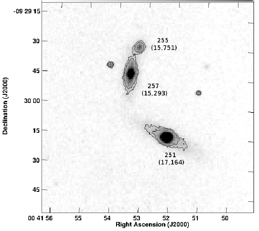
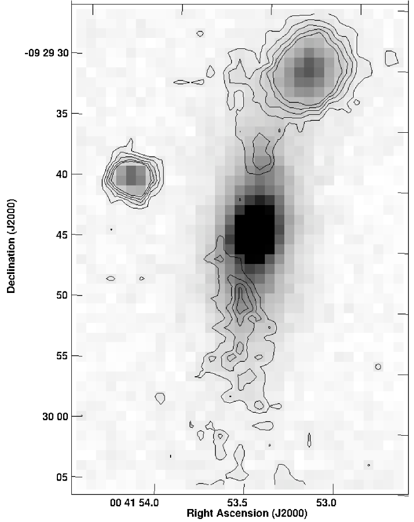
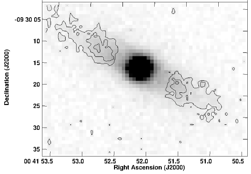
Figure 10: Field 9: A triplet around [DFL98]257. Top left panel: J-band in contours and grey scale. The first contour corresponds to 3.5 times the $rms$ background level. The names of the galaxies are given according to Table 2. Velocities (in  km s^-1) are given in parentheses. Top right: close up of A85[DFL98]257; the residual image is shown in contours, overlaid on the J-band image. Bottom: Residual image of A85[DFL98]251, in contours. The strong asymmetries seen around the two massive spirals suggests that they are part of a physical triplet, with the low mass galaxy A85[DFL98]255.

Field 9, the triplet A85[DFL98]251/255/257: This field is projected onto the $South\,Blob$ (BA09), lying some 10^′  (600 kpc) south of the cluster center. Three galaxies appear very close in projection from each other (see Fig. 10), A85[DFL98]251/257/255, two giant spirals and a low mass elliptical, respectively. The first one is an early spiral (Sa), lying at the SW of this trio; it has a radial velocity larger by 1,400  km s^-1  than the other two galaxies, making unclear if it is physically linked with the close pair A85[DFL98]255/257. Now we show that both the large spirals (i.e. A85[DFL98]251/257) display significant asymmetries in NIR (${\alpha}_{A3}$= 0.14, 0.32, respectively), giving support to a recent flyby $\leq 0.25\times 10^{8}$ yrs ago (estimated in the same way as previously). On the other hand, the galaxies A85[DFL98]255/257, have a relative velocity of only ${\sim}$450  km s^-1  (see Table 2), making very likely that they constitute a physical pair, probably in contact. The southern component, the spiral A85[DFL98]257, displays enhanced H$\alpha$ emission (BA09), suggesting that a burst of star formation could have been triggered by tidal interactions with its neighbors. It is worth mentioning that none of the two large spirals in this field (A85[DFL98]251,257) were detected in   (BA09), down to an -mass detection threshold of 7$\times$10⁸ M_⊙. This suggests that, lying well within the $SouthBlob$, these galaxies could have suffered strong RPS in addition to the observed tidal interactions. This could explain the absence of gas in both spirals.

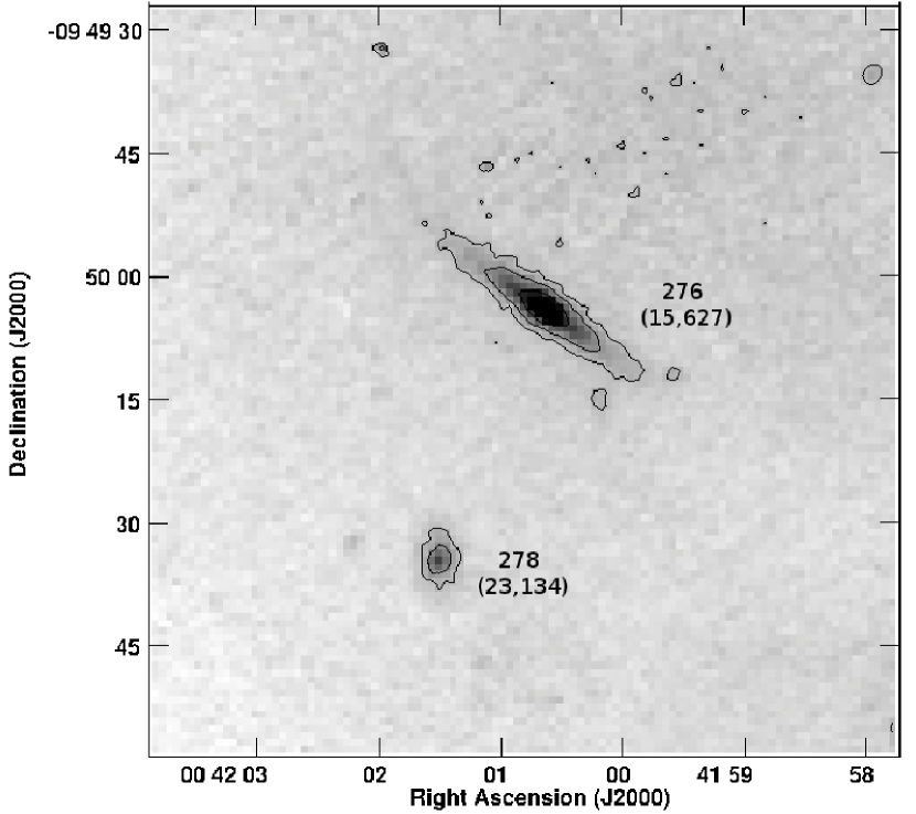
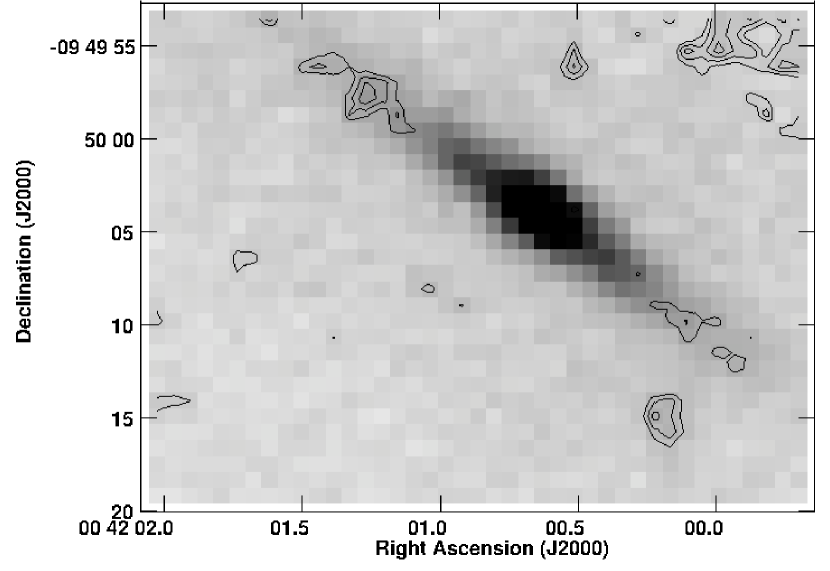
Figure 11: Field 10, centered on the isolated galaxy A85[DFL98]276. Left panel: J-band in contours and grey scale. The first contour corresponds to 3.5 times the $rms$ background level. The names of the galaxies are given according to Table 2. Velocities (in  km s^-1) are given in parentheses. Right panel: The residual image is shown in contours, overlaid on the J-band image. Important asymmetries are shown on both sides of the disk. The NW corner of the panel was affected by a slightly inhomogeneous background, having no effects on our asymmetry analysis.

Field 10, the isolated galaxy A85[DFL98]276: This field hosts a bright (Sb) spiral. In spite of its projection, nearly 2 Mpc south of the cD, and far from the detected X-ray emission, this galaxy is very gas deficient as no   was detected below an -mass detection threshold of 7$\times$10⁸M_⊙  (see BA09). Furthermore, a stellar disk with slight asymmetries on both sides, appears from our NIR analysis, with a larger elongation to the NE (see Fig. 11). No direct neighbor can be linked to this galaxy, as the closest object in projection, (A85[DFL98]278), has a radial velocity of 23,134  km s^-1. No cluster substructures are reported in this area, making this perturbed galaxy, a very intriguing one. This evidence suggests, assuming a radial orbit, that A85[DFL98]276 could be subject to galaxy harassment (Moore et al., 1996) along that cluster passage.

Fields 11-15, two very disrupted galaxies: Several objects have been previously reported (BA09) in A 85 as showing extremely blue colors, with only a few of them being detected in . Several of these galaxies appear very distorted in blue light, the most striking cases are A85[DFL98]176 (see Field 2, above), and A85[DFL98]286/374.

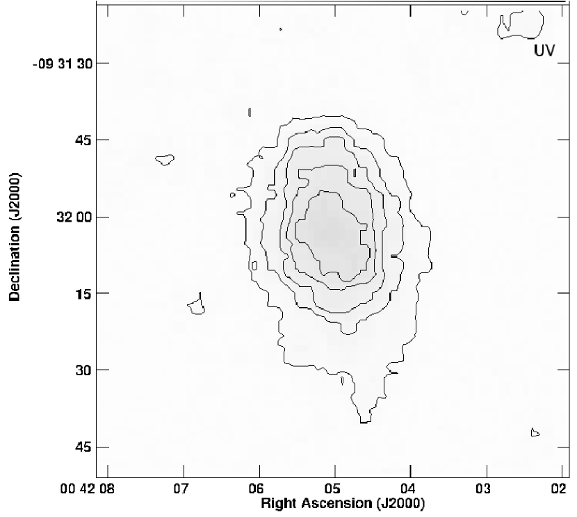
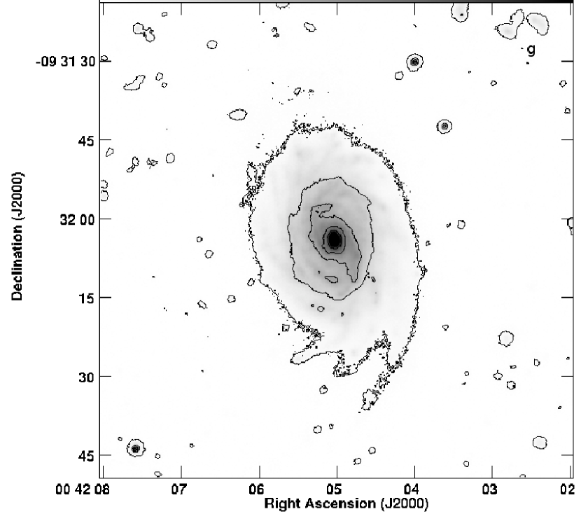
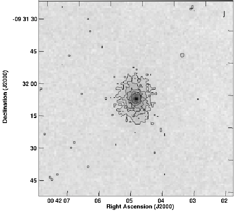
Figure 12: The $jellyfish$ galaxy A85[DFL98]286 (MCG-02-02-091), seen in near-UV (GALEX, top left), optical (MEGACam-g, top right) and J-band (bottom) images. No asymmetries are seen in the NIR, while very strongly disrupted arms appear in blue light to the south.

A85[DFL98]286 (MCG-02-02-091) is projected onto our Field 11, lying 0.9 Mpc south of the cluster center. This galaxy is a nearly face-on spiral, projected on the edge of the South Blob, within a relatively high density ICM region. In principle this could explain the -deficiency as it was not detected by our VLA-  survey (BA09 and Bravo-Alfaro et al. 2017, in prep.) This galaxy shows disrupted arms when seen in UV and in blue images, and it has been cataloged as a $jellyfish$ galaxy by Poggianti et al. (2016). Fig. 12 shows that the length of the extended arms is shorter in A85[DFL98]286, compared with A85[DFL98]176. Very interestingly, none of these galaxies shows old stars in NIR along the disrupted arms. Finally, no global asymmetry is obtained through our NIR analysis (${\alpha}_{A3}$= 0.03); these results suggest that RPS is playing the most important role producing the strong observed disruption seen in A85[DFL98]286.

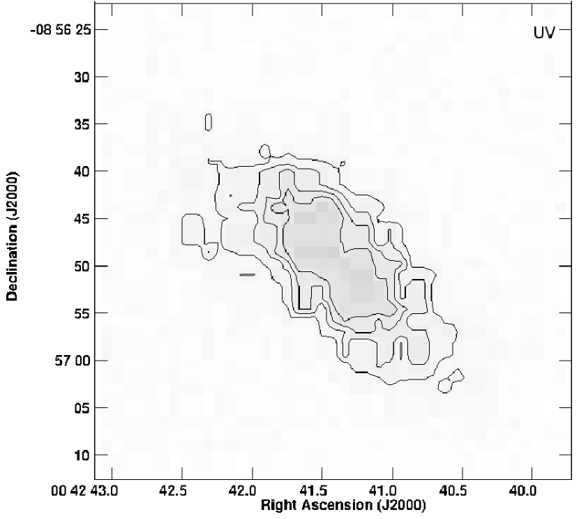
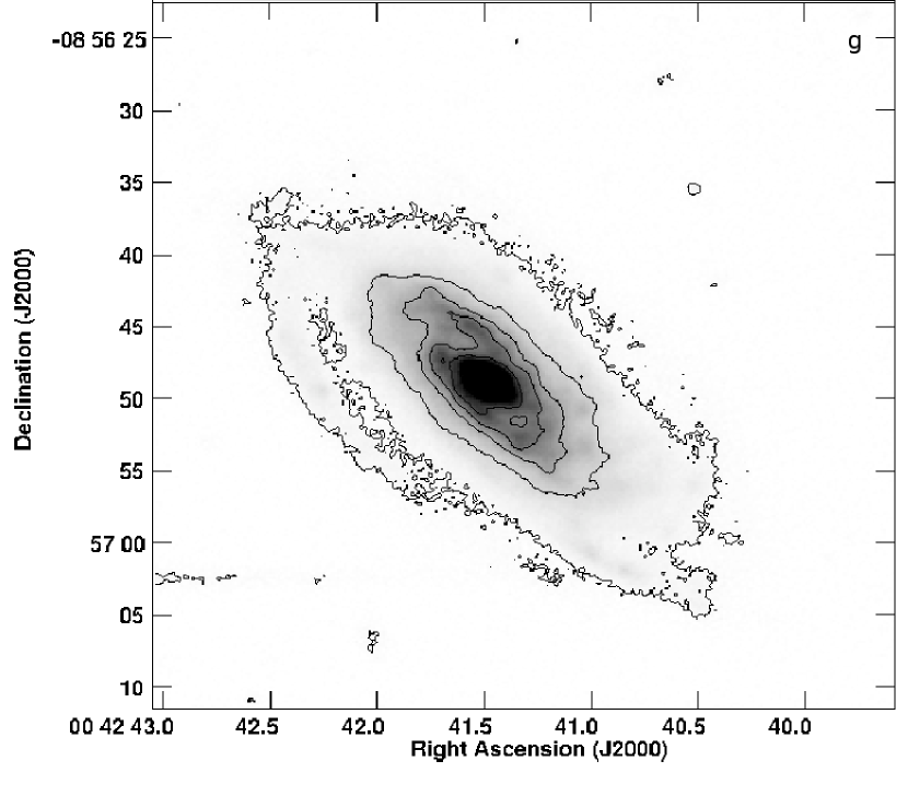
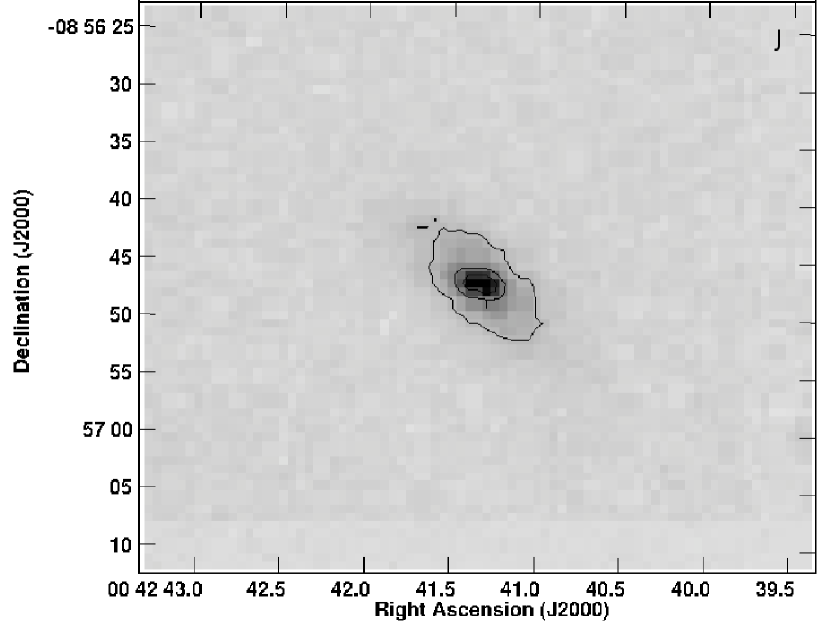
Figure 13: A85[DFL98]374, a candidate to $jellyfish$, seen in near-UV (GALEX, top left), optical (MEGACam-g, top right) and J-band (bottom) images. This is a rich -galaxy, projected 1.5 Mpc, NE of the cluster center. A very strong variation of the P.A. is observed in NIR, as a function of radius. Nevertheless, no external asymmetries are seen in NIR compared with the strongly disrupted arms appearing in blue light, to the SW.

Another remarkable case among the blue and disrupted galaxies is A85[DFL98]374, which may well be a third $jellyfish$ galaxy in A 85. This object was observed within our field 15, some 1.5 Mpc NE of the cluster center (Fig. 1). The strong disruption seen through visual inspection in the UV and optical bands (see Fig. 13), follows the pattern seen in the two $jellyfish$ galaxies described above. Nevertheless, A85[DFL98]374 could be in an earlier stage of disruption compared with A85[DFL98]176/286: first, the elongated arms in A85[DFL98]374, on the SW, are less ”developed” and are shorter than in the other two disrupted objects. And second, this galaxy still shows a high   content (Bravo-Alfaro et al. 2017, in prep.). Concerning the NIR, A85[DFL98]374 appears very symmetric (${\alpha}_{A3}$= 0.02) and no red stars are seen along the disrupted arms, just like in the two $jellyfish$ galaxies. So, a strong RPS event could be at the very first stages of sweeping gas away from the disk, forming new stars along the gas tails. In view of the large distance from the cluster center, a high speed relative to the cluster is needed for RPS to be efficient. In their analysis of RPS vs cluster-centric distance in A85, BA09 showed that relative velocities above 1,000 km s^-1  are necessary for RPS to overcome the restitution force exerted on the -gas, at the projected distance of A85[DFL98]374.

5 Summary and Conclusions

Our main results are summarized as follows:

1. With the aim of unveiling and studying specific cases of tidally disrupted objects in Abell 85, we observed 26 fields in the NIR, 3^′$\times$3^′  in size, and obtained accurate J, H, K’-photometry for 68 bright galaxies. Our apperture NIR magnitudes are in close agreement with 2MASS, with our images being ${\sim}$1 mag arcsec^-2 deeper. Our J, H, K’ atlas of images are available upon request.

2. With the aim of providing quantitative information on the presence (and degree) of tidal disruptions, we propose a new asymmetry index, ${\alpha}_{An}$. From the sample of 68 galaxies, we selected the 41 largest in angular size, in order to go through an asymmetry analysis. Our index is able to measure (in surface) the asymmetry features in a galaxy. This tool proved to deliver important complementary information to that provided by other indices available in the literature.

3. Among 41 bright galaxies going through our asymmetry analysis we report 10 objects showing mild-to-strong asymmetries. For a few of the disrupted objects, asymmetries could be seen through visual inspection on our NIR images. Nevertheless, our method unveiled unexpected asymmetry features associated with other galaxies, confirming the efficiency of the residual technique. We quantified the degree of asymmetry with the ${\alpha}_{A3}$  index, finding that these perturbations go from mild (${\alpha}_{A3}$ = 1.0) to strong (1.1$\leq$ ${\alpha}_{A3}$ $\leq$ 0.32). We compared the residuals coming from the $bmodel$ and the 180^∘-rotation method, and found that the first method delivers a systematically higher asymmetry index. Even considering our biased sample, it is important to notice that the fraction of disrupted galaxies among the brightest objects of A 85, is already close to 25%. This confirms that gravitational mechanisms are playing a role in transforming galaxies in this cluster.

4. We combined our NIR study with previous results of substructures found in A 85. The asymmetries measured in the NIR allowed to confirm the presence of some physical pairs and groups, linked with larger structures. For instance, galaxies observed in our Fields 2 and 3, are projected onto the same substructure, $C2$ (BA09), some 200-300 kpc west of the cluster center. If we consider that this structure is believed to be infalling from the background with a high velocity relative to the cluster, then the galaxies within this group would be undergoing galaxy $pre-processing$ before reaching the main cluster body, accounting for the slight asymmetries observed in NIR. Since the velocity dispersion among the objects within this group is large (above 1,000  km s^-1), they might constitute a loose group of galaxies. Another case is observed within our Field 9, where three galaxies are projected within the $South\,Blob$ (BA09). The significant NIR asymmetries, measured on the two giant spirals, strongly suggest that they have been in contact, probably through a flyby interaction, less than 10⁸ years ago.

5. A very interesting issue we approached in this paper was the deep NIR imaging of three very disrupted (two of them being classified as $jellyfish$) galaxies in A 85: A85[DFL98]176/ 286/374. We have shown that comparing the NIR morphology with the UV-optical delivers very useful physical information about such disrupted galaxies. The three objects display different degrees of morphological disruption, A85[DFL98]176 being the most dramatic case. This kind of galaxies are well known to display disrupted arms, being very bright in UV and blue bands. We have shown that the disrupted arms are not detected in the NIR bands, in spite of our deep images going down to 22.4 mag arcsec^-2 (in J-band). This absence of old stars along the disrupted arms discards any tidal interaction as the origin of the perturbation: gravitational interactions would tear up all kind of stars from the galaxy disk, both blue and red ones. Our results support the hypothesis that a very strong RPS event, observed at different stages along the three objects, is responsible for the galaxy disruption and formation of the arms/tails. In this scenario RPS removed a large fraction of the -gas, and the bright stars seen in UV-optical are formed along the gas tails.

We have shown that combining deep NIR imaging with other datasets, such as optical imaging and redshifts, as well as substructures in clusters, constitutes a powerful tool to investigate the recent evolution of galaxies infalling into such massive systems. We have also shown that measuring asymmetries allows to quantify the degree of interaction a galaxy is undergoing. All this sheds light on the role played by environment, and by different physical mechanisms driving the infall and evolution of galaxies in clusters. In our forthcoming papers we will combine detailed   information (maps, gas content, kinematics) with homogeneous optical/NIR imaging, both covering large volumes of a sample of nearby clusters.

Table 1: The fields observed in NIR in A 85

Field	$\alpha_{J2000}$	$\delta_{J2000}$	Year	Obj	$t$ (sec)	Notes
					J, H, K’
(1)	(2)	(3)	(4)	(5)	(6)	(7)
1	00 41 19.8	-09 23 27	2007, 2009	150	3260 3240 3380	pair/-def
2	00 41 30.3	-09 15 46	2007, 2009	176	3480 3240 3510	group
3	00 41 35.1	-09 21 52	2009	197	2280 2340 3780	group
4	00 41 36.1	-08 59 36	2010,2011	201	2700 2700 3240	pair/-def
5	00 41 39.6	-09 14 57	2010	209	2160 2160 2700	pair
6	00 41 40.1	-09 18 15	2009	210	1620 1620 3780	pair
7	00 41 43.0	-09 26 22	2009	221	1800 1980 2640	group/-def
8	00 41 50.5	-09 18 11	2009	242	1620 1740 2640	cD
9	00 41 53.2	-09 29 29	2006,2011	255	2520 2520 2520	group/-def
10	00 42 00.6	-09 50 04	2006	276	2640 2640 3600	isolated
11	00 42 05.0	-09 32 04	2006,2011	286	3840 3840 2850	pair/-def
12	00 42 18.7	-09 54 14	2006,2010	323	2700 3240 3240	-rich
13	00 42 24.2	-09 16 17	2010	338	2160 2160 2700	pair/-def
14	00 42 29.5	-10 01 07	2006	347	3600 3975 3540	-rich
15	00 42 41.5	-08 56 49	2007	374	2630 3490 3655	group/-rich
16	00 42 43.9	-09 44 21	2011	382	2160 2160 2160	pair/-def
17	00 42 48.4	-09 34 41	2011	391	2160 2160 2160	-def
18	00 43 01.6	-09 47 34	2006,2010	426	3804 3480 3240	group/-rich
19	00 43 10.1	-09 51 41	2006,2011	442	3000 3800 2890	group/-def
20	00 43 11.6	-09 38 16	2006	451	3300 3000 3000	pair/-def
21	00 43 14.3	-09 10 21	2007	461	2430 4100 3700	blue/-rich
22	00 43 19.5	-09 09 13	2007	*3114	3600 3600 3600	blue/-rich
23	00 43 31.2	-09 51 48	2006	486	3800 3800 2840	blue/-rich
24	00 43 34.0	-08 50 37	2007	491	3240 3800 3800	blue/-rich
25	00 43 38.7	-09 31 21	2006	496	3780 3660 3720	blue/-rich
26	00 43 43.9	-09 04 23	2007	502	3240 3500 3600	blue/-rich

Note. — Column (1): the field number, ordered by R.A. Columns (2) and (3): the center of each field. Column (4): the year(s) of the corresponding observing run. Column (5): the galaxy used as reference within each field; names are taken from (Durret et al., 1998a), except (*), coming from (Slezak et al., 1998). Column (6): total integration times, for each band, in seconds. Column (7): Notes about the interest associated with each field; see text.

Table 2: Optical data of the observed galaxies in A 85

Field	Galaxy	$\alpha_{2000}$, $\delta_{2000}$	Vel.	Opt.	Diam.	Morph.
			(km/s)	magn.	(′)
(1)	(2)	(3)	(4)	(5)	(6)	(7)
1	145	00 41 19.0, -09 23 24	14,935	17.9	0.21	-
	150	00 41 19.8, -09 23 27	14,681	16.5r	0.30	-
2	167	00 41 27.1, -09 13 42	14,167	16.7	0.25	-
	*1645	00 41 27.9, -09 13 47	16,315	17.1	0.78	-
	174	00 41 28.8, -09 13 59	13,997	15.4v	0.50	-
	176	00 41 30.3, -09 15 46	13,393	15.1	0.37	cD*
	177	00 41 30.4, -09 14 07	16,328	15.5v	0.20	-
	186	00 41 33.3, -09 14 57	17,566	16.9	0.36	-
3	175	00 41 30.5, -09 21 33	16,365	17.7	0.34	-
	182	00 41 32.0, -09 20 03	13,794	16.3	0.37	-
	192	00 41 34.7, -09 21 00	17,358	16.3	0.24	-
	195	00 41 34.9, -09 21 38	17,103	18.1	0.19	-
	197	00 41 35.0, -09 21 51	14,236	16.6	0.46	-
4	193	00 41 34.9, -09 00 47	17,556	17.4	0.26	-
	201	00 41 36.2, -08 59 35	17,935	16.8	0.56	-
5	206	00 41 39.0, -09 27 48	17,126	18.4	0.19	-
	209	00 41 39.6, -09 27 31	16,666	17.6	0.30	-
6	202	00 41 36.2, -09 19 30	16,371	17.3	0.21	-
	210	00 41 40.1, -09 18 15	16,825	17.5	0.20	-
	214	00 41 41.3, -09 18 57	14,283	16.5	0.40	-
7	215	00 41 41.4, -09 26 21	16,305	18.4	0.14	-
	221	00 41 43.0, -09 26 22	16,886	14.8	1.00	-
	222	00 41 43.5, -09 25 30	16,923	18.3	0.21	-
	243	00 41 50.2, -09 25 47	17,349	15.8	0.53	E
8	*1895	00 41 45.5, -09 16 35	$\cdots$	19.8	-	-
	236	00 41 48.2, -09 17 03	15,870	16.3	0.35	-
	*1951	00 41 49.6, -09 17 43	14,995	16.0	0.21	-
	242	00 41 50.5, -09 18 11	16,690	14.7b	1.30	cD
	*1966	00 41 50.7, -09 17 39	16,536	18.8v	-	-
9	238	00 41 49.1, -09 29 03	18,367	17.0r	0.18	-
	251	00 41 52.1, -09 30 15	17,164	14.5r	0.30	Sa
	254	00 41 53.1, -09 31 16	17,121	17.6i	0.24	-
	255	00 41 53.2, -09 29 29	15,751	16.2v	0.47	E
	257	00 41 53.5, -09 29 44	15,293	16.0	0.72	Sc
10	276	00 42 00.6, -09 50 04	15,627	16.4	0.81	Sb
	278	00 42 01.5, -09 50 35	23,134	17.5	0.26	S
11	286	00 42 05.0, -09 32 04	15,852	15.9	0.68	Sc
	*2260	00 42 08.3,-09 31 05	16,963	17.8r	0.19	-
12	315	00 42 16.1, -09 54 28	38,609	18.3	0.18	S0
	323	00 42 18.7, -09 54 14	15618	17.9	0.31	-
	*2423	00 42 21.1, -09 54 29	$\cdots$	19.4	0.12	-
13	322	00 42 18.7, -09 15 28	16,732	16.6	0.41	-
	338	00 42 24.2, -09 16 16	18,195	17.1	0.25	-
14	347	00 42 29.5, -10 01 07	15,165	17.7	0.29	-
15	374	00 42 41.5, -08 56 49	15,106	16.5	0.56	-
	377	00 42 42.2, -08 55 28	16,992	16.6	0.43	-
	385	00 42 44.2, -08 56 12	16,150	16.6	0.31	-
16	366	00 42 37.0, -09 45 20	17,065	17.8r	0.21	-
	372	00 42 40.2, -09 44 17	16,922	17.8r	0.31	S0
	382	00 42 43.9, -09 44 21	15,231	17.1	0.39	Sb
17	*2746	00 42 48.1, -09 34 54	$\cdots$	19.2	0.18	-
	391	00 42 48.4, -09 34 41	17,940	17.7	0.33	-
18	426	00 43 02.0, -09 46 40	14,734	17.3	0.18	-
19	423	00 43 01.4, -09 51 31	15,333	17.0	0.41	S0
	*2923	00 43 04.9, -09 51 38	$\cdots$	20.1	0.08	-
	*2934	00 43 05.0, -09 51 11	$\cdots$	18.8	0.13	-
	435	00 43 06.0, -09 50 15	14,742	16.7	0.37	Sb
	*2950	00 43 06.4, -09 51 40	17,727	18.2	0.24	-
	439	00 43 08.2, -09 49 37	15,203	17.2	0.22	-
	442	00 43 10.1, -09 51 41	15,142	15.3	0.68	E/S0
20	447	00 43 10.9, -09 40 53	16,492	15.8	0.51	E
	451	00 43 11.6, -09 38 16	16,253	15.8	0.48	Sb
21	461	00 43 14.3, -09 10 21	15,015	18.4	0.28	-
22	3114	00 43 19.5, -09 09 13	15,060	19.2	0.13	-
23	486	00 43 31.2, -09 51 48	16,619	16.8	0.52	S
	*3234	00 43 32.6, -09 51 52	$\cdots$	19.7	0.12	-
24	491	00 43 34.0, -08 50 37	14,968	17.0	0.33	-
	*3260	00 43 35.1, -08 51 13	$\cdots$	19.0	0.17	-
25	*3270	00 43 35.1, -09 32 14	$\cdots$	19.4	0.14	-
	496	00 43 38.7, -09 31 21	15,004	17.0	0.34	-
26	502	00 43 43.9, -09 04 23	15,004	16.8	0.40	-

Note. — Optical data obtained from the NED database (http://ned.ipac.caltech.edu). Columns (1) and (2): ID for the field and the galaxies, respectively, using the same names and references of Table 1. Column (3): R.A., Dec for each galaxy. Column (4): Optical radial velocity. Column (5): g-magnitude from NED; otherwise the band is indicated. Column (6): Major angular diameter, in arcmins. Column (7) Morphological type, when available. cD* : This object is wrongly classified; it is a spiral object (see Sect. 4.2)

Table 3: The NIR magnitudes of observed galaxies in A 85.

ID	$J$	$H$	$K^{\prime}$	$J_{2MASS}$	$H_{2MASS}$	$K_{2MASS}$
(1)	(2)	(3)	(4)	(5)	(6)	(7)
145	14.54	16.09	16.07	-	-	-
150	14.65	14.37	13.41	-	-	-
167	14.05	13.57	13.07	14.099	13.382	13.024
*1645	14.77	14.15	13.79	14.866	14.085	13.888
174	13.47	13.07	12.54	13.549	12.794	12.531
176	13.44	12.69	12.48	13.397	12.720	12.384
177	13.14	12.56	12.15	13.212	12.468	12.145
186	13.96	13.20	12.76	14.039	13.300	12.977
175	14.61	14.02	13.71	-	-	-
182	13.78	13.17	12.92	13.820	13.156	12.789
192	13.99	13.43	12.85	14.162	13.450	13.116
195	14.88	14.42	14.03	15.083	14.619	13.866
197	13.19	12.69	12.33	13.409	12.784	12.410
193	15.28	14.34	14.05	15.147	14.356	13.707
201	14.43	13.94	13.83	14.551	14.084	13.475
206	15.83	15.45	14.92	-	-	-
209	14.37	13.55	13.59	14.388	13.767	13.299
202	14.39	13.70	13.36	14.273	13.573	13.132
210	13.89	13.17	12.83	13.767	13.089	12.738
214	14.07	13.44	13.36	14.110	13.413	13.202
215	14.98	15.51	14.32	-	-	-
221	13.21	12.42	12.17	13.188	12.512	12.092
222	15.41	16.18	14.52	-	-	-
243	13.16	12.44	12.02	13.169	12.418	12.070
*1895	15.22	14.64	14.92	-	-	-
236	13.34	12.59	12.53	13.394	12.644	12.333
*1951	14.94	14.30	14.30	-	-	-
242	12.96	12.24	11.99	12.856	12.082	11.741
*1966	16.66	16.29	16.61	-	-	-
238	14.91	14.48	14.87	-	-	-
251	13.12	12.49	12.19	13.199	12.465	12.146
254	14.93	14.60	13.92	14.986	14.428	14.054
255	14.74	14.15	14.21	-	-	-
257	13.56	12.91	12.75	13.634	12.885	12.587
276	14.12	13.26	12.74	14.110	13.304	12.986
278	15.23	14.34	13.97	15.172	14.347	13.993
286	14.24	13.39	13.39	14.172	13.535	13.219
*2260	16.16	17.92	18.35	-	-	-
315	15.45	14.50	14.21	15.521	14.532	14.013
*2423	15.97	16.04	14.97	-	-	-
322	13.88	13.12	12.69	13.828	13.107	12.797
338	14.76	14.05	13.83	14.681	14.026	13.533
347	16.32	15.10	15.70	-	-	-
374	14.32	13.53	13.72	14.353	13.600	13.396
377	13.92	13.14	13.25	14.021	13.392	13.117
385	14.02	13.26	13.01	14.059	13.256	13.068
366	16.82	15.68	14.59	-	-	-
372	14.75	14.01	13.93	14.898	14.148	13.807
382	14.53	13.84	13.68	14.531	13.765	13.490
*2746	15.71	15.01	14.64	-	-	-
391	15.80	15.41	15.06	-	-	-
426	14.51	13.89	13.66	14.661	13.858	13.698
423	14.55	13.60	13.05	14.353	13.608	13.367
*2923	16.77	15.92	15.43	-	-	-
*2934	16.48	15.71	15.30	-	-	-
435	14.08	13.44	12.97	14.067	13.281	13.014
*2950	16.60	16.03	15.56	-	-	-
439	14.59	13.93	13.43	14.495	13.808	13.380
442	13.02	12.06	12.03	12.949	12.233	11.956
447	13.53	12.92	12.84	13.571	12.877	12.572
451	13.91	13.27	13.08	13.804	13.084	12.778
486	15.68	14.97	14.77	-	-	-
*3234	17.83	16.21	16.17	-	-	-
491	15.65	15.24	14.84	-	-	-
*3260	16.38	16.09	16.14	-	-	-
*3270	16.88	15.77	15.48	-	-	-
496	15.91	14.88	15.03	-	-	-
502	16.31	15.59	15.21	-	-	-

Note. — Column (1): Galaxy names, as in Table 2. Columns (2), (3), (4): NIR (J,H,K’), 14^′′  aperture magnitudes obtained in the present work. Columns (5), (6), (7): NIR (J,H,K’), 14^′′  aperture magnitudes from 2MASS, when available, for comparison.

Table 4: Asymmetry index for selected galaxies in A 85.

ID	J-H	${\alpha}_{A3}$	Position	Dist(Mpc)
(1)	(2)	(3)	(4)	(5)
150	0.53	0.032	C2	0.62
167	0.44	0.070	C2	0.49
174	0.52	0.010	C2	0.41
175	0.60	0.050	M	0.35
176	0.64	0.140	C2	0.33
177	0.82	0.110	M	0.37
182	0.61	0.049	C2	0.29
186	0.65	0.070	M	0.32
193	0.85	0.050		1.19
197	0.68	0.250	C2	0.31
201	0.79	0.150		1.26
209	0.78	0.040	SB	0.58
214	0.59	0.030	C2	0.14
221	0.72	0.045	SB	0.56
236	0.76	0.050	M	0.07
242	0.64	0.062	M	0.0
243	0.69	0.059	SB	0.45
251	0.65	0.140	SB	0.79
255	0.56	0.037	SB	0.77
257	0.64	0.320	SB	0.78
276	0.79	0.110		1.80
278	0.82	0.100		1.95
286	0.79	0.030	SB	0.96
322	0.73	0.023	M	0.45
338	0.72	0.017	M	0.58
347	0.65	0.040		2.93
372	0.71	0.100	SE	1.80
374	0.65	0.020		1.66
377	0.63	0.040		1.20
382	0.65	0.190	SE	1.96
385	0.69	0.020		1.21
391	0.50	0.030		1.46
423	0.72	0.020	SE	1.80
435	0.73	0.025	SE	2.48
442	0.84	0.041	SE	2.50
447	0.68	0.060	SE	2.02
451	0.67	0.004	SE	1.90
486	0.69	0.030	SE	2.79
491	0.54	0.040		2.52
496	0.50	0.010		2.00
502	0.59	0.010		2.10

Note. — Asymmetry index for the galaxies being larger than 0.25^′. Column (1): galaxy name, as in previous tables. Column (2): (J-H) color index. Column (3): the ${\alpha}_{A3}$  index, after applying the $bmodel$ residual. Column (4): the projected position of each galaxy, following the code used in (BA09) for the substructures reported across A 85. Galaxies for which a $Position$ is not given, are considered at the outskirts of the cluster. Column (5): projected cluster-centric distance, in Mpc.

Figure 4: Comparison of ${\alpha}_{A3}$  with the visual asymmetry index ($dist$) defined by Nair & Abraham (2010). Twenty galaxies spanning the full range of disruption were chosen. Unperturbed galaxies display index values close to zero in both systems, showing that ${\alpha}_{A3}$ successfully separate symmetric from disrupted objects; the dotted line separates the former from the later, in our ${\alpha}_{A3}$  system. A trend is clear where both indices increase with stronger asymmetry features.

Figure 5: Histogram showing the distribution of asymmetry index values for our sub-sample of 41 galaxies (see Table 4). Ten of these objects display significant asymmetries, corresponding to index values ${\alpha}_{A3}$ $>$ 0.1.

References

- Abraham et al. (2003) Abraham, R. G., van den Bergh, S., & Nair, P. 2003, ApJ, 588, 218
- Adams et al. (2012) Adams, S. M., Zaritsky, D., Sand, D. J., et al. 2012, AJ, 144, 128
- Bamford et al. (2009) Bamford, S. P., Nichol, R. C., Baldry, I. K., et al. 2009, MNRAS, 393, 1324
- Barway et al. (2007) Barway, S., Kembhavi, A., Wadadekar, Y., et al. 2007, ApJ, 661, L37
- Barway et al. (2005) Barway, S., Mayya, Y. D., Kembhavi, A. K., et al. 2005, AJ, 129, 630
- Bedregal et al. (2006) Bedregal, A. G., Aragón-Salamanca, A., Merrifield, M. R., et al. 2006, MNRAS, 371, 1912
- Bellhouse et al. (2017) Bellhouse, C., Jaffé, Y. L., Hau, G. K. T., et al. 2017, ApJ, 844, 49
- Bertin & Arnouts (1996) Bertin, E., & Arnouts, S. 1996, A&AS, 117, 393
- Boselli & Gavazzi (2006) Boselli, A., & Gavazzi, G. 2006, PASP, 118, 517
- Bravo-Alfaro et al. (2000) Bravo-Alfaro, H., Cayatte, V., van Gorkom, J. H., et al. 2000, AJ, 119, 580
- Bravo-Alfaro et al. (2001) Bravo-Alfaro, H., Cayatte, V., van Gorkom, J. H., et al. 2001, A&A, 379, 347
- Bravo-Alfaro et al. (2009) Bravo-Alfaro, H., Caretta, C. A., Lobo, C., et al. 2009, A&A, 495, 379 (BA09)
- Byrd & Valtonen (1990) Byrd, G., & Valtonen, M. 1990, ApJ, 350, 89
- Calvi et al. (2012) Calvi, R., Poggianti, B. M., Fasano, G., et al. 2012, MNRAS, 419, L14
- Chung et al. (2007) Chung, A., van Gorkom, J. H., Kenney, J. D. P., et al. 2007, ApJ, 659, L115
- Chung et al. (2009) Chung, A., van Gorkom, J. H., Kenney, J. D. P., et al. 2009, AJ, 138, 1741
- Conselice (2003) Conselice, C. J. 2003, ApJS, 147, 1
- Conselice (2014) Conselice, C. J. 2014, ARA&A, 52, 291
- Cortese et al. (2007) Cortese, L., Marcillac, D., Richard, J., Bravo-Alfaro, H. et al. 2007, MNRAS, 376, 157
- Crowl et al. (2005) Crowl, H. H., Kenney, J. D. P., van Gorkom, J. H., et al. 2005, AJ, 130, 65
- Cruz-González et al. (1994) Cruz-González, I., Carrasco, L., Ruiz, E., et al. 1994, Rev. Mexicana Astron. Astrofis., 29, 197
- Dressler (1980) Dressler, A. 1980, ApJ, 236, 351
- Durret et al. (1998a) Durret, F., Felenbok, P., Lobo, C., et al. 1998a, A&AS, 129, 281
- Durret et al. (1998b) Durret, F., Forman, W., Gerbal, D., et al. 1998b, A&A, 335, 41
- Ebeling et al. (2014) Ebeling, H., Stephenson, L. N., & Edge, A. C. 2014, ApJ, 781, L40
- Erwin et al. (2012) Erwin, P., Gutiérrez, L., & Beckman, J. E. 2012, ApJ, 744, L11
- Gunn & Gott (1972) Gunn, J. E., & Gott, J. R. 1972, ApJ, 176, 1
- Hawarden et al. (2001) Hawarden, T. G., Leggett, S. K., Letawsky, M. B., et al. 2001, MNRAS, 325, 563
- Holwerda et al. (2014) Holwerda, B. W., Muñoz-Mateos, J.-C., Comerón, S., et al. 2014, ApJ, 781, 12
- Ichinohe et al. (2015) Ichinohe, Y., Werner, N., Simionescu, A., et al. 2015, MNRAS, 448, 2971
- Jaffé et al. (2011) Jaffé, Y. L., Aragón-Salamanca, A., Kuntschner, H., et al. 2011, MNRAS, 417, 1996
- Jaffé et al. (2016) Jaffé, Y. L., Verheijen, M. A. W., Haines, C. P., et al. 2016, MNRAS, 461, 1202
- Jarrett et al. (2003) Jarrett, T. H., Chester, T., Cutri, R., et al. 2003, AJ, 125, 525
- Jedrzejewski (1987) Jedrzejewski, R. I. 1987, MNRAS, 226, 747
- Kenney et al. (2004) Kenney, J. D. P., van Gorkom, J. H., & Vollmer, B. 2004, AJ, 127, 3361
- Kodama & Smail (2001) Kodama, T., & Smail, I. 2001, MNRAS, 326, 637
- Koopmann & Kenney (2004) Koopmann, R. A., & Kenney, J. D. P. 2004, ApJ, 613, 866
- Lewis et al. (2002) Lewis, I., Balogh, M., De Propris, R., et al. 2002, MNRAS, 334, 673
- Lotz et al. (2004) Lotz, J. M., Primack, J., & Madau, P. 2004, AJ, 128, 163
- Mayya et al. (2005) Mayya, Y. D., Carrasco, L. & Luna, A. 2005, ApJ, 628, L33
- McIntosh et al. (2004) McIntosh, D. H., Rix, H.-W., & Caldwell, N. 2004, ApJ, 610, 161
- McPartland et al. (2016) McPartland, C., Ebeling, H., Roediger, E., et al. 2016, MNRAS, 455, 2994
- Merritt (1983) Merritt, D. 1983, ApJ, 264, 24
- Mihos et al. (2005) Mihos, J. C., Harding, P., Feldmeier, J., et al. 2005, ApJ, 631, L41
- Moore et al. (1996) Moore, B., Katz, N., & Lake, G. 1996, ApJ, 457, 455
- Nair & Abraham (2010) Nair, P. B., & Abraham, R. G. 2010, ApJS, 186, 427
- Persson et al. (1998) Persson, S. E., Murphy, D. C., Krzeminski, W., et al. 1998, AJ, 116, 2475
- Plauchu-Frayn & Coziol (2010) Plauchu-Frayn, I. & Coziol, R. 2010, AJ, 139, 2643
- Poggianti & van Gorkom (2001) Poggianti, B. M., & van Gorkom, J. H. 2001, Gas and Galaxy Evolution, 240, 599
- Poggianti et al. (2016) Poggianti, B. M., Fasano, G., Omizzolo, A., et al. 2016, AJ, 151, 78
- Rawle et al. (2013) Rawle, T. D., Lucey, J. R., Smith, R. J., et al. 2013, MNRAS, 433, 2667
- Romano et al. (2008) Romano, R., Mayya, Y. D., & Vorobyov, E. I. 2008, AJ, 136, 1259
- Scott et al. (2010) Scott, T. C., Bravo-Alfaro, H., Brinks, E., et al. 2010, MNRAS, 403, 1175
- Scott et al. (2012) Scott, T. C., Cortese, L., Brinks, E., et al. 2012, MNRAS, 419, L19
- Slezak et al. (1998) Slezak, E., Durret, F., Guibert, J., & Lobo, C. 1998, A&AS, 128, 67
- Valentinuzzi et al. (2009) Valentinuzzi, T., Woods, D., Fasano, G., et al. 2009, A&A, 501, 851
- van Dokkum (2005) van Dokkum, P. G. 2005, AJ, 130, 2647
- Yoshida et al. (2012) Yoshida, M., Yagi, M., Komiyama, Y., et al. 2012, ApJ, 749, 43
- Yu et al. (2016) Yu, H., Diaferio, A., Agulli, I., et al. 2016, ApJ, 831, 156