DESY 17-091

The Toric SO(10) F-Theory Landscape


W. Buchmuller${}^{\,\text{a}}$, M. Dierigl${}^{\,\text{a}}$, P.-K. Oehlmann${}^{\,\text{a}}$ and F. Ruehle${}^{\,\text{b}}$

${}^{\text{a}}$ Deutsches Elektronen-Synchrotron DESY, Notkestr. 85, 22607 Hamburg, Germany
${}^{\text{b}}$ Rudolf Peierls Centre for Theoretical Physics, Oxford University,
1 Keble Road, Oxford, OX1 3NP, UK

Supergravity theories in more than four dimensions with grand unified gauge symmetries are an important intermediate step towards the ultraviolet completion of the Standard Model in string theory. Using toric geometry, we classify and analyze six-dimensional F-theory vacua with gauge group SO(10) taking into account Mordell-Weil U(1) and discrete gauge factors. We determine the full matter spectrum of these models, including charged and neutral SO(10) singlets. Based solely on the geometry, we compute all matter multiplicities and confirm the cancellation of gauge and gravitational anomalies independent of the base space. Particular emphasis is put on symmetry enhancements at the loci of matter fields and to the frequent appearance of superconformal points. They are linked to non-toric Kähler deformations which contribute to the counting of degrees of freedom. We compute the anomaly coefficients for these theories as well by using a base-independent blow-up procedure and superconformal matter transitions. Finally, we identify six-dimensional supergravity models which can yield the Standard Model with high-scale supersymmetry by further compactification to four dimensions in an Abelian flux background.

1 Introduction

F-theory [1, 2, 3] provides a fascinating geometric picture of fundamental forces and matter. Gauge interactions, matter fields and their interactions are all encoded in the singularities of elliptically fibered Calabi-Yau (CY) manifolds: Codimension-one singularities determine non-Abelian gauge groups, codimension-two singularities yield the representations of matter fields [4, 5] and codimension-three singularities their Yukawa couplings [6].

Although the main ingredients of F-theory have been known for two decades, significant progress towards realistic low energy effective theories have only been made much later by searching for F-theory vacua that incorporate higher-dimensional grand unified theories (GUTs) [6, 7, 8, 9, 10]. Making use of the geometry of del Pezzo surfaces and U(1) fluxes of intersecting D7-branes, an interesting class of semi-realistic local GUT models has been constructed (for reviews, see [11, 12, 13]). These local models were then extended to global GUT models which incorporate gravity, and therefore the full geometry of the CY manifolds on which F-theory is compactified [14, 15, 16].

However, despite the remarkable progress in F-theory model building in recent years, a number of important conceptual and phenomenological questions still remain open. In fact, to the best of our knowledge, at present there is no fully satisfactory F-theory GUT model, which would have to account for symmetry breaking to the standard model gauge group, the matter content of the (supersymmetric) standard model, doublet-triplet splitting, sufficiently suppressed proton decay, supersymmetry breaking and semi-realistic quark and lepton mass matrices. For example, the usually employed hypercharge flux breaking generically leads to massless exotic states [17, 18], although this might be avoided in some models [19] based on a classification of SU(5)$\times$U(1) matter charges accomplished in [20]. Important progress has been made towards implementing Wilson line breaking [21] but a realistic model still remains to be found. Note that interesting supersymmetric extensions of the Standard Model have also been obtained without the GUT paradigm [22, 23, 24, 25].

The present paper was motivated by a six-dimensional (6d) supergravity (SUGRA) model with gauge group SO(10)$\times$U(1) [26], based on previous work on orbifold GUTs with Wilson lines[27, 28, 29, 30]. U(1) gauge flux in the compact dimensions plays an important twofold role. It generates a multiplicity of quark-lepton generations, and it breaks supersymmetry [31]. Compactifying to four dimensions, this leads to multiplets split with respect to either supersymmetry or the GUT symmetry, a picture reminiscent of ‘split supersymmetry’ [32, 33] or ‘spread supersymmetry’ [34]. From heterotic string compactifications it is known that six-dimensional SUGRA theories can emerge as an intermediate step in the compactification to four dimensions [35, 36, 37, 38]. 6d string vacua with GUT gauge symmetries have also been extensively studied in F-theory (for reviews see, e.g. [39, 40]). It is then natural to ask whether models of this type can be embedded into F-theory or whether they belong to the ‘swampland’ [41]. In this work we therefore classify a set of 6d global F-theory models with gauge group SO(10) and some additional gauge factors of small rank.

Recently, F-theory was also used as an efficient tool to describe more exotic phenomena like tensionless strings in a consistent manner. These sectors are realized in F-theory fibrations where the fiber develops a so-called (4,6,12) singularity in codimension-two in the base. In six dimensions these singularities have a physical interpretation in terms of superconformal field theories [42] related to tensionless strings[43]. Following [44] we refer to these singularities as superconformal points (SCP). They can be viewed as pairs of colliding singularities, which can be separated by blow-ups in the base. These blow-ups yield new tensor multiplets and one obtains a CY manifold without SCPs [45]. The new tensors couple to the string with a coupling strength given by the size of the blow-up cycle. When the fiber is fully resolved in codimension one it becomes non-flat over these codimension-two points [46, 47, 48]. This means that the dimension of the fiber jumps and contains higher dimensional components. In [46] it was then observed that the presence of (4,6,12) singularities implies non-flatness of the resolved fibration. These points are more likely to be present in theories with large gauge groups, such as SO(10). Hence, as we are considering resolved SO(10) models, we indeed encounter many theories with superconformal points, present as non-flat fibers in codimension two. In this analysis we also study these theories, i.e. matter representations, anomaly cancellation and relations to other theories via tensionless string transitions [45] in global F-theory models over an arbitrary base.

In the following we systematically study 6d F-theory with gauge symmetry SO(10) and additional low-rank group factors. Our starting point is the base-independent analysis of all toric hypersurface fibrations in [49], together with the classification of all tops leading to non-Abelian gauge groups in [50]. Some global SO(10) models have already been studied in [51, 52, 53]. In our work we extend this to all toric models with torus fibrations described by a single hypersurface, which includes fibrations with discrete groups, Mordell-Weil U(1) factors [54] and additional non-Abelian gauge groups over arbitrary bases.

In our analysis of the 6d F-theory vacua we determine the complete massless matter spectra, including all SO(10) singlets and non-flat fibers points, i.e. SCPs, using geometric computations only. For all theories we confirm cancellation of gauge and gravitational anomalies and we provide the anomaly coefficients base-independently. We find a total number of 36 different models with additional U(1) symmetries up to rank three, as well as $\mathbb{Z}_{2}$ and $\mathbb{Z}_{3}$ discrete symmetries that are of possible phenomenological interest after further compactification to four dimensions. In particular for the models with discrete gauge symmetries, we compute singlet multiplicities and discrete charges of SO(10) matter multiplets. Furthermore, we discuss the connection of fibrations with different SO(10) tops via conifold transitions in the generic fiber.

In total around 80% of the models contain SCPs, for which the fiber becomes non-flat. For those theories we carry out a base-independent blow-up procedure and provide the anomaly coefficients as well. In the computation of the full spectrum, we find an important new contribution of non-toric Kähler deformations coming from the non-flat fiber points that correspond to 6d tensors and have to be taken into account for the correct counting of neutral singlets. Furthermore, we show that theories with non-flat fibers are connected to tops that have points in the interior of a face which can often be reached via tensionless string transition from another top with no superconformal points. In these transitions we again show the appearance of non-toric Kähler deformations in the fiber in the computation of base-independent Euler numbers. In particular we discuss these transitions for the first time in global theories with additional (discrete) Abelian gauge factors over an arbitrary base.

Our analysis is strongly based on previous studies of SU(5) vacua [56, 57, 58, 47, 59, 60]. In Section 2 we describe the various steps of the calculation in detail for one example, a torus given by the polygon $F_{3}$ [61], which allows for a U(1) factor. Fibering the ambient space $X_{F_{3}}$ over $\mathbb{P}^{1}$, we construct a $K3$ manifold which can be tuned to have an SO(10) singularity according to the Kodaira classification [62]. Resolving this singularity with an SO(10) top produces five $\mathbb{P}^{1}$s which, together with the torus, show the intersection pattern of the extended SO(10) Dynkin diagram. Particular emphasis is given to the symmetry enhancements at codimension-two and codimension-three singularities, which yield the loci of matter fields and Yukawa couplings. We find the standard pattern of extended Dynkin diagrams but also some non-Kodaira fibers generically present where matter curves self-intersect [63, 64]. To complete the analysis, the multiplicities of matter fields are computed for the Hirzebruch base $\mathbb{F}_{0}=\mathbb{P}^{1}\times\mathbb{P}^{1}$.

In Section 3 a base-independent analysis is performed and the matter multiplicities are evaluated as intersection numbers on the base. A challenging problem is the computation of the SO(10) singlet spectra. We obtain the multiplicities of all charged and neutral singlets. This is achieved by unhiggsing the gauge group SO(10)$\times$U(1) to SO(10)$\times$U(1)² as an intermediate step where the computations are feasible.

Section 4 contains the main result of the paper, the classification and analysis of all 6d toric SO(10) vacua. We briefly review the structure of the fibers describing a torus in different ambient spaces [61] and the SO(10) tops that can be added to the various polygons [50]. In total there are 36 different models. Using the techniques that were exemplified in Section 2 and 3, we then calculate all matter representations, compute their multiplicities and confirm cancellation of all anomalies in a base-independent manner for each model. A complete list of these data is given in Appendix C. An interesting outcome of our classification is the frequent appearance of SCPs. We identify these points as an additional source of (1,1)-forms in the fiber, which is important for counting all neutral degrees of freedom. After the separation of the codimension-two colliding singularities via a blow-up in the base we confirm cancellation of all anomalies in these theories as well. Moreover, we discuss the connection of these theories via higgsings and tensionless string transitions.

Section 5 is devoted to 6d supergravity models with gauge group SO(10)$\times$U(1) which are phenomenologically promising. These models contain one charged ${\bf 16}$-plet that yields the quark-lepton generations as zero modes in an Abelian flux compactification, and additional uncharged ${\bf 16}$-plets needed for $B-L$ breaking. In addition, these models have several neutral ${\bf 10}$-plets which, via doublet-triplet splitting, yield two Higgs doublet superfields in the 4d effective theory. We first consider the model in [26] and show that, after adding charged and neutral SO(10) singlets, all anomalies can be canceled. This model, however, is not contained in our classification and therefore belongs to the ‘toric swampland’. On the other hand, variants of this model with charged ${\bf 10}$-plets, which have additional vector-like matter, can be obtained as 6d F-theory vacua.

A summary of our results and a brief discussion of unsolved challenging problems are presented in Section 6. Appendix A gives more details required for a full understanding of the example discussed in Section 2 and 3. In Appendix B polynomials and divisor classes are given for the fibers $F_{2}$ and $F_{4}$, as well as the expressions for the functions $f$ and $g$ needed to obtain the elliptic curves in Weierstrass form. Appendix C contains the data of the 36 models contained in our analysis. Finally, in Appendix D a list of phenomenologically viable models is given.

2 A 6d vacuum with gauge group SO(10)$\times$U(1)

In this section we discuss the explicit geometric construction of a specific global F-theory model with gauge group SO(10)$\times$U(1). Moreover, we evaluate its matter spectrum, Yukawa couplings and anomaly coefficients in full detail.

2.1 Torus with non-trivial Mordell-Weil group

Our starting point is an elliptic curve $\mathcal{E}$ with a Mordell-Weil group of rank one, which yields a U(1) gauge group when fibered over an appropriate base space. This is the case for the torus contained in the two-dimensional toric ambient space $dP_{1}$ which can be parametrized by four homogeneous coordinates $[u:v:w:e_{1}]$, with two independent $\mathbb{C}^{*}=(\mathbb{C}-\{0\})$ scale transformations modded out.

In order to obtain the elliptic curve $\mathcal{E}$ inside the ambient space $dP_{1}$, one first chooses the corresponding toric ambient space polygon [61], $F_{3}$, where each homogeneous coordinate is associated with a two-dimensional vector (see Figure 1, Table 1).

Figure 1: The polygon $F_{3}$ describing a torus in the ambient space $dP_{1}$.

One then constructs the dual polygon $F_{3}^{*}$ which, together with $F_{3}$, defines the the polynomial $p_{F_{3}}$ (see Appendix A),

$$p_{F_{3}}= \ s_{1}u^{3}e_{1}^{2}+s_{2}u^{2}ve_{1}^{2}+s_{3}uv^{2}e_{1}^{2}+s_{4}v^{3}e_{1}^{2}+s_{5}u^{2}we_{1}$$

$$+s_{6}uvwe_{1}+s_{7}v^{2}we_{1}+s_{8}uw^{2}+s_{9}vw^{2}\,.$$ (2.1)

This polynomial defines a torus in the toric ambient space,

$$\mathcal{E}=\{p_{F_{3}}=0\}\,,$$ (2.2)

with the coefficients $s_{1},\ldots,s_{9}$ being generic complex numbers. The vanishing of the homogeneous coordinates $u$, $v$, $w$ and $e_{1}$ defines four divisors

$$D_{u}\,\,,D_{v}\,\,,D_{w}\,\,,D_{e_{1}}\,,$$ (2.3)

where $D_{x_{i}}=\{x_{i}=0\}$.

$\begin{array}[]{|c|c|c|cc|}\hline\cr\text{coordinates}&\text{vertices}&\text{divisor classes}&[v]&[e_{1}]\\ \hline\cr\hline\cr u&(1,-1)&[v]&0&1\\ v&(-1,0)&[v]&0&1\\ w&(0,1)&[ve_{1}]&1&0\\ e_{1}&(0,-1)&[e_{1}]&1&-1\\ \hline\cr\end{array}$

Table 1: Coordinates, vertices, divisor classes and intersection numbers (charges of $\mathbb{C}^{*}$-actions) for the two-dimensional toric variety $dP_{1}$.

Since the ambient space $dP_{1}$ is two-dimensional there are two linear dependencies,

$$\sum_{i}Q_{ai}D_{x_{i}}\sim 0\,,\quad a=1,2\,,$$ (2.4)

where $Q_{ai}$ are the charges of the two $\mathbb{C}^{*}$-actions. In Table 1 we have also listed the intersection numbers of the two divisor classes $[v]$ and $[e_{1}]$ with all divisors. One easily verifies that these intersection numbers play the role of the charges of the two $\mathbb{C}^{*}$-actions, $x_{i}\rightarrow\lambda^{Q_{ai}}x_{i}$ with $\lambda\in\mathbb{C}^{*}$, under which the polynomial $p_{F_{3}}$ transforms homogeneously. Using the linear dependencies the two remaining divisor classes can be expressed in terms of the two independent ones,

$$[u]=[v]\,,\quad[w]=[v]+[e_{1}]=[ve_{1}]\,.$$ (2.5)

The torus $\mathcal{E}$ has a ‘zero-point’ $P_{0}$ which is obtained as intersection with the divisor $D_{e_{1}}$. On this divisor $w$ can be set to one by a $\mathbb{C}^{*}$-action (see Appendix A), which yields for the coordinates of $P_{0}$

$$\hat{s}_{0}=D_{e_{1}}\cap\mathcal{E}:\ [s_{9},-s_{8},1,0]\,.$$ (2.6)

There exists a second rational point $P_{1}$ on the torus (see Figure 2), which can be obtained from the a tangent $t_{P}$ at $P_{0}$ along the torus [49],

$$\hat{s}_{1}=\{t_{P}=0\}\cap\mathcal{E}\,,\quad t_{P}=s_{8}u+s_{9}v\,.$$ (2.7)

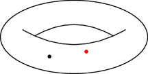
Figure 2: The elliptic curve $\mathcal{E}$ with two points, $\hat{s}_{0}$ and $\hat{s}_{1}$ (see text).

The Mordell-Weil group then defines an addition, $P_{0}\rightarrow P_{0}+P_{1}\rightarrow P_{0}+2P_{1}\rightarrow\ldots$. For a fibration of the torus over some base the points $\hat{s}_{0}$ and $\hat{s}_{1}$ become functions of the base coordinates and define a divisor which corresponds to the generator of a continuous U(1) symmetry. The divisor is obtained from $[\hat{s}_{0}]$ and $[\hat{s}_{1}]$ and can be written as [54]

$$\sigma_{1}\equiv[\hat{s}_{1}]-[\hat{s}_{0}]=[v]-[e_{1}]\,,$$ (2.8)

where we have represented the tangent $t_{P}$ by the divisor class $[v]$.

2.2 $\boldsymbol{K3}$ manifold

Now we describe the construction of a $K3$ manifold with an SO(10) singularity leading to the desired gauge group of the model as well as its resolution to a smooth CY twofold.

Singular limit

We fiber the elliptic curve $\mathcal{E}$ over some base space, in the simplest case a $\mathbb{P}^{1}$. This is achieved by extending the two-dimensional ambient space to a three-dimensional ambient space for which we choose a polyhedron with vertices given in Table 2. The homogeneous coordinates of the base $\mathbb{P}^{1}$ are $z_{0}$ and $z_{1}$.

Like for the ambient space $dP_{1}$, one can determine the dual polytope and the polynomial $p_{\hat{Y}_{2}}$ that defines a CY twofold $\hat{Y}_{2}$ via $\hat{Y}_{2}=\{p_{\hat{Y}_{2}}=0\}$. The polynomial $p_{\hat{Y}_{2}}$ turns out to consist of 28 monomials corresponding to a smooth $K3$ manifold (see Appendix A). Tuning ten of them to zero yields the following factorization (see (2.1)):

$$\begin{split}s_{1}&=d_{1}z_{0}\,,\;s_{2}=d_{2}z_{0}^{2}\,,\;s_{3}=d_{3}z_{0}^{2}\,,\;s_{4}=d_{4}z_{0}^{3}\,,\;s_{5}=d_{5}\,,\\ s_{6}&=d_{6}z_{0}\,,\;s_{7}=d_{7}z_{0}\,,\;s_{8}=d_{8}\phantom{z_{0}^{2}}\,,\;s_{9}=d_{9}\,.\end{split}$$ (2.9)

The coefficients $d_{1},\ldots d_{9}$ are homogeneous functions of the base coordinates, $d_{i}=d_{i}(z_{0},z_{1})$ (see Appendix A).

For the three-dimensional toric variety $dP_{1}$ fibered over $\mathbb{P}^{1}$ one can define curves as intersections of divisors with the CY twofold $\hat{Y}_{2}$. From the two independent divisor classes $[v]$ and $[e_{1}]$, and the base coordinate $[z_{0}]$, one obtains the curves $\mathcal{C}_{v}$, $\mathcal{C}_{e_{1}}$ and $\mathcal{C}_{b}$:

$$\begin{array}[]{l|l c}\,\text{curves}&\quad\quad\text{intersections}&\text{coordinate patch}\\ \hline\cr\quad\mathcal{C}_{v}&v\cap(d_{1}e_{1}^{2}z_{0}+d_{5}e_{1}w+d_{8}w^{2})&u=1\\ \quad\mathcal{C}_{e_{1}}&e_{1}\cap(d_{8}u+d_{9}v)&w=1\\ \quad\mathcal{C}_{b}&z_{0}\cap(d_{5}e_{1}u^{2}+d_{8}u+d_{9}v)&z_{1}=1\\ \hline\cr\end{array}$$ (2.14)

In Table 2 we have listed the intersection numbers of these curves with fiber and base divisors,

$$[v]\cdot\mathcal{C}_{v}\,,\quad[v]\cdot\mathcal{C}_{e_{1}}\,,\quad[v]\cdot\mathcal{C}_{b}\,,\ldots$$ (2.15)

Note that the self-intersections of the divisors on the smooth CY twofold are $[v]\cdot\mathcal{C}_{v}=-2$ and $[e_{1}]\cdot\mathcal{C}_{e_{1}}=-2$. Hence, these curves correspond to two $\mathbb{P}^{1}$s.

$\begin{array}[]{|c|c|c|ccc|}\hline\cr\text{coordinates}&\text{vertices}&\text{divisor classes}&\mathcal{C}_{v}&\mathcal{C}_{e_{1}}&\mathcal{C}_{b}\\ \hline\cr\hline\cr u&(1,-1,0)&[vz_{0}]&0&2&2\\ v&(-1,0,0)&[v]&-2&1&2\\ w&(0,1,0)&[ve_{1}z_{0}]&1&0&3\\ e_{1}&(0,-1,0)&[e_{1}]&1&-2&1\\ z_{0}&(0,0,1)&[z_{0}]&2&1&0\\ z_{1}&(-1,0,-1)&[z_{0}]&2&1&0\\ \hline\cr\end{array}$

Table 2: Coordinates, vertices, divisor classes and intersection numbers (charges of $\mathbb{C}^{*}$-actions) for the three-dimensional toric variety $dP_{1}$ fibered over $\mathbb{P}^{1}$.

For the chosen values of the parameters of $p_{\hat{Y}_{2}}$, and therefore the sections $s_{i}$, the CY twofold $\hat{Y}_{2}$ develops singularities that can be related to non-Abelian groups according to the Kodaira classification. To study these singularities one first uses a standard procedure [65] that brings the torus (2.1) to Weierstrass form,

$$F=-y^{2}+x^{3}+fx+g=0\,.$$ (2.16)

Here $x$ and $y$ are certain functions of the homogeneous coordinates $u$, $v$, $w$ and $e_{1}$, and the coefficients $f$ and $g$ are functions of the base coordinates $z_{0}$ and $z_{1}$, $d_{i}(z_{0},z_{1})$. Expanding the sections $d_{i}$ (see (A.10)) around $z_{0}=0$, $d_{i}(z_{0},z_{1})=d_{i}+\mathcal{O}(z_{0})$, and using Eqs. (B.24) and (B.25), we find

$$\begin{split}f=&z_{0}^{2}\left(-\frac{1}{3}d_{5}^{2}d_{7}^{2}+z_{0}R_{1}+\mathcal{O}(z_{0}^{2})\right)\,,\\ g=&z_{0}^{3}\left(-\frac{2}{27}d_{5}^{3}d_{7}^{3}+z_{0}R_{2}+\mathcal{O}(z_{0}^{2})\right)\,,\end{split}$$ (2.17)

where $R_{1}$ and $R_{2}$ are polynomials in the sections $d_{i}$. The torus is singular at a point $(x,y)$ when

$$F=\frac{\partial F}{\partial x}=\frac{\partial F}{\partial y}=0\,.$$ (2.18)

This is the case when the discriminant $\Delta$ vanishes,

$$\Delta=4f^{3}+27g^{2}=0\,.$$ (2.19)

From Eqs. (2.17), (2.19) and the expressions for $R_{1,2}$ one obtains

$$\Delta=z_{0}^{7}(P+z_{0}R+\mathcal{O}(z_{0}^{2}))\,,$$ (2.20)

where

$$P=-d_{5}^{3}d_{7}^{3}(d_{3}d_{5}-d_{1}d_{7})^{2}d_{9}^{2}\,,$$ (2.21)

and $R$ is a generic polynomial of degree 16 in the $d_{i}$ . Clearly, at the base coordinate $z_{0}=0$ the torus is singular at $(x,y)=(0,0)$. The order (Ord) of this codimension-one singularity is characterized by the power in $z_{0}$ of $f$, $g$ and $\Delta$. From Eqs. (2.17) and (2.19) we infer an $\text{Ord}(f,g,\Delta)=(2,3,7)$ singularity which corresponds to the gauge group SO(10) [62].

For a higher-dimensional base the sections $d_{i}$ depend on additional coordinates and can possibly vanish at certain points of the base where in addition to $z_{0}$ one of the $d_{i}$’s vanishes. According to Eqs. (2.17) and (2.20) the vanishing of some $d_{i}$’s enhances the singularity of the torus at $z_{0}=0$. Generically, this corresponds to larger symmetries according to the Kodaira classification. The relevant cases are summarized in Table 3. These codimension-two singularities will be analyzed in more detail in Section 2.3.

$\begin{array}[]{| c | c | c|}\hline\cr\text{locus}&\text{Ord}(f,g,\Delta)&\text{fiber singularity}\\ \hline\cr\hline\cr z_{0}=0&(2,3,7)&SO(10)\\ \hline\cr z_{0}=d_{9}=0&(2,3,8)&SO(12)\\ z_{0}=d_{5}=0&(3,4,8)&E_{6}\\ z_{0}=d_{7}=0&(3,4,8)&E_{6}\\ z_{0}=d_{3}d_{5}-d_{1}d_{7}=0&(2,3,8)&SO(12)\\ \hline\cr\end{array}$

Table 3: Codimension-one and codimension-two singularities of the CY twofold and the associated symmetry groups.

Resolved $\boldsymbol{K3}$ manifold

To analyze the gauge symmetries and the matter content encoded in the singular $K3$ manifold, one has to resolve the singularities. This is achieved by adding an SO(10) ‘top’ [66] to the polytope following the classification of [50]. Since the gauge group has rank $5$, five new coordinates are introduced, which yield five additional divisor classes,

$$\{D_{1},\ldots,D_{5}\}=\{[f_{2}],[g_{1}],[g_{2}],[f_{3}],[f_{4}]\}\,.$$ (2.22)

The vertices of the polytope are listed in Table 4. The dual polytope has 18 vertices (see Appendix A), and the sections $s_{i}$ in the polynomial (2.1) take the form

$$\begin{array}[]{lll}s_{1}=d_{1}z_{0}f_{2}^{2}f_{4}g_{1}\,,&s_{2}=d_{2}z_{0}^{2}f_{2}^{2}f_{3}f_{4}g_{1}^{2}g_{2}\,,&s_{3}=d_{3}z_{0}^{2}f_{2}f_{3}g_{1}\,,\\ s_{4}=d_{4}z_{0}^{3}f_{2}f_{3}^{2}g_{1}^{2}g_{2}\,,&s_{5}=d_{5}f_{2}f_{4}\,,&s_{6}=d_{6}z_{0}f_{2}f_{3}f_{4}g_{1}g_{2}\,,\\ s_{7}=d_{7}z_{0}f_{3}\,,&s_{8}=d_{8}f_{2}f_{3}f_{4}^{2}g_{1}g_{2}^{2}\,,&s_{9}=d_{9}f_{3}f_{4}g_{2}\,,\end{array}$$ (2.26)

where now the sections $d_{i}$ depend on the coordinates $z_{1}$ and $z$,

$$d_{i}=d_{i}(z,z_{1})\,,\quad z=z_{0}f_{2}g_{1}^{2}g_{2}^{2}f_{3}f_{4}\,.$$ (2.27)

The polynomial (2.1) together with (2.26) defines a CY twofold $Y_{2}$ where the singularities of the tuned CY twofold $\hat{Y}_{2}$ have been resolved. The divisor $\{z_{0}=0\}$ is now replaced by the divisor $\{z=0\}$ which is the sum of the base divisor $\{z_{0}=0\}$ and the fiber divisors $\{f_{2}=0\},\ldots,\{g_{2}=0\}$, i.e. $\{z=0\}$ differs from $\{z_{0}=0\}$ by the sum of the SO(10) Cartan divisors. Correspondingly, for $Y_{2}$ the divisors $D_{z}$ and $D_{z_{1}}$ belong to the same divisor class (see Table 4) whereas for $\hat{Y}_{2}$ the divisors $D_{z_{0}}$ and $D_{z_{1}}$ belong to the same class (see Table 2).

The polynomial obtained from Eqs. (2.1) and (2.26) reads explicitly

$$\begin{split}p_{Y_{2}}=&d_{1}u^{3}e_{1}^{2}z_{0}f_{2}^{2}f_{4}g_{1}+d_{2}u^{2}ve_{1}^{2}z_{0}^{2}f_{2}^{2}f_{3}f_{4}g_{1}^{2}g_{2}+d_{3}uv^{2}e_{1}^{2}z_{0}^{2}f_{2}f_{3}g_{1}\\ &+d_{4}v^{3}e_{1}^{2}z_{0}^{3}f_{2}f_{3}^{2}g_{1}^{2}g_{2}+d_{5}u^{2}we_{1}f_{2}f_{4}+d_{6}uvwe_{1}z_{0}f_{2}f_{3}f_{4}g_{1}g_{2}\\ &+d_{7}v^{2}we_{1}z_{0}f_{3}+d_{8}uw^{2}f_{2}f_{3}f^{2}_{4}g_{1}g_{2}^{2}+d_{9}vw^{2}f_{3}f_{4}g_{2}\,.\end{split}$$ (2.28)

It defines a $K3$ manifold with resolved SO(10) singularity and will be the basis of the following calculations.

$\begin{array}[]{|c|c|c|cccccccc|}\hline\cr\text{coordinates}&\text{vertices}&\text{divisor classes}&\mathcal{C}_{v}&\mathcal{C}_{e_{1}}&\mathbb{P}^{1}_{0}&\mathbb{P}^{1}_{1}&\mathbb{P}^{1}_{2}&\mathbb{P}^{1}_{3}&\mathbb{P}^{1}_{4}&\mathbb{P}^{1}_{5}\\ \hline\cr\hline\cr u&(1,-1,0)&[vz_{0}g_{1}g_{2}f_{3}]&0&2&0&1&0&0&0&1\\ v&(-1,0,0)&[v]&-2&1&1&0&0&0&1&0\\ w&(0,1,0)&[ve_{1}z_{0}g_{2}^{-1}f_{4}^{-1}]&0&0&0&0&0&1&0&1\\ e_{1}&(0,-1,0)&[e_{1}]&1&-2&1&0&0&0&0&0\\ f_{2}&(1,0,1)&D_{1}&0&0&0&-2&1&0&0&0\\ g_{1}&(1,1,2)&D_{2}&0&0&1&1&-2&1&0&0\\ g_{2}&(1,2,2)&D_{3}&0&0&0&0&1&-2&1&1\\ f_{3}&(0,1,1)&D_{4}&1&0&0&0&0&1&-2&0\\ f_{4}&(1,1,1)&D_{5}&0&0&0&0&0&1&0&-2\\ z_{0}&(0,0,1)&D_{0}&1&1&-2&0&1&0&0&0\\ z_{1}&(-1,0,-1)&[z]&2&1&0&0&0&0&0&0\\ \hline\cr z&&[z]&2&1&0&0&0&0&0&0\\ \hline\cr\end{array}$

Table 4: Coordinates, vertices, divisor classes and intersection numbers (charges of $\mathbb{C}^{*}$-actions) for the three-dimensional toric variety $dP_{1}$ with SO(10) top, fibered over $\mathbb{P}^{1}$. The divisor $[z]$ is given by $[z_{0}f_{2}g_{1}^{2}g_{2}^{2}f_{3}f_{4}]$.

The presence of additional exceptional divisors changes the linear dependencies. The divisor classes $[u]$ and $[w]$ can now be written as (see Appendix A)

$$[u] =[v]+D_{0}+D_{2}+D_{3}+D_{4}\,,$$ (2.29)

$$[w] =[v]+[e_{1}]+D_{0}-D_{3}-D_{4}\,.$$ (2.30)

The intersection of the divisors $D_{v}$, $D_{e_{1}}$, $D_{0}$, $\ldots$, $D_{5}$ with the CY twofold $Y_{2}$ defines a set of curves that are given in Table 5. For each divisor certain coordinates can be set to one (see Appendix A), which simplifies the calculations. The intersection numbers of divisor classes $[x_{i}]$ and curves $C_{j}=x_{j}\cap p_{Y_{2}}$ correspond to the intersections of two divisors on the CY twofold,

$$[x_{i}]\cdot C_{j}=C_{i}\cdot[x_{j}]=[x_{i}]\cdot[p_{Y_{2}}]\cdot[x_{j}]\,.$$ (2.31)

All intersection numbers are given in Table 4. Note that self-intersection numbers of the divisors on the CY twofold, i.e. the intersection numbers of the divisors $[v]$, $\ldots$,$D_{5}$ with the associated curves $\mathcal{C}_{v}$, $\ldots$,$\mathbb{P}^{1}_{5}$, are all equal to $-2$. The curves $\mathcal{C}_{v}$ and $\mathcal{C}_{e_{1}}$ are base $\mathbb{P}^{1}$s whereas $\mathbb{P}^{1}_{0}$ to $\mathbb{P}^{1}_{5}$ lie in the fiber.

Particularly interesting are the intersections numbers of the divisors that were introduced to resolve the SO(10) singularity. From Table 4 one reads off

$$D_{i}\cdot\mathbb{P}^{1}_{j}=\mathbb{P}^{1}_{i}\cdot D_{j}=-(C_{SO(10)})_{ij}\,,\quad i,j=1,\ldots 5\,,$$ (2.32)

$\begin{array}[]{|c|l l|}\hline\cr\text{curves}&\text{intersections}&\text{coordinate patches}\\ \hline\cr\hline\cr\mathcal{C}_{v}&v\cap(d_{1}e_{1}^{2}z_{0}+d_{5}we_{1}+d_{8}w^{2}f_{3})&(u,f_{2},g_{1},g_{2},f_{4})=1\\ \mathcal{C}_{e_{1}}&e_{1}\cap(d_{8}u+d_{9}v)&(w,f_{2},g_{1},g_{2},f_{3},f_{4})=1\\ \mathbb{P}^{1}_{0}&z_{0}\cap(d_{8}f_{2}f_{3}g_{1}u+d_{5}e_{1}f_{2}u^{2}+d_{9}f_{3}v)&(w,f_{4},g_{2})=1\\ \mathbb{P}^{1}_{1}&f_{2}\cap(d_{7}z_{0}+d_{9}f_{4})&(v,e_{1},w,f_{3},g_{2})=1\\ \mathbb{P}^{1}_{2}&g_{1}\cap(d_{7}z_{0}f_{3}+d_{5}f_{2}f_{4}+d_{9}f_{3}f_{4}g_{2})&(u,v,w,e_{1})=1\\ \mathbb{P}^{1}_{3}&g_{2}\cap(d_{3}f_{3}g_{1}+d_{1}f_{4}g_{1}+d_{7}f_{3}w+d_{5}f_{4}w)&(u,v,e_{1},z_{0},f_{2})=1\\ \mathbb{P}^{1}_{4}&f_{3}\cap(d_{1}z_{0}g_{1}+d_{5}w)&(e_{1},u,f_{2},f_{4})=1\\ \mathbb{P}^{1}_{5}&f_{4}\cap(d_{4}f_{2}g_{1}^{2}g_{2}+d_{3}f_{2}g_{1}u+d_{7}w)&(v,e_{1},z_{0},f_{3})=1\\ \hline\cr\end{array}$

Table 5: Curves on the CY twofold $Y_{2}$ defined as intersections of divisors with $Y_{2}$. On each divisor the coordinates enclosed in $(\ldots)$ can be set to one by $\mathbb{C}^{*}$-actions.

Figure 3: The extended Dynkin diagram of SO(10) obtained from intersections of divisors $D_{I}$ and curves $\mathbb{P}^{1}_{J}$, with $I,J\in\{0,\ldots,5\}$. Intersections of the torus divisors $[e_{1}]$ and $[v]$ are also indicated.

where

$$C_{SO(10)}=\left(\begin{array}[]{ccccc}2&-1&0&0&0\\ -1&2&-1&0&0\\ 0&-1&2&-1&-1\\ 0&0&-1&2&0\\ 0&0&-1&0&2\end{array}\right)$$ (2.38)

is the SO(10) Cartan matrix. Hence, the divisors $D_{i}$ are referred to as Cartan divisors. Together with the divisor $D_{0}$ of the base coordinate $z_{0}$, the Cartan divisors have the intersection numbers corresponding to the extended Dynkin diagram of SO(10) (see Table 4, Figure 3). One easily verifies that the intersection numbers of the 8 curves $\mathcal{C}_{v}$,…,$\mathbb{P}^{1}_{5}$ with the 11 divisors $[u]$,…,$[z_{1}]$ represent the charges of the 8 $\mathbb{C}^{*}$-scalings that leave the CY twofold $Y_{2}$ invariant.

The exceptional torus divisor $[e_{1}]$ only intersects the affine node,

$$[e_{1}]\cdot\mathbb{P}^{1}_{I}=(1,0,0,0,0,0)_{I}\,,\quad I=0,\ldots,5\,,$$ (2.39)

whereas the divisor $[v]$ intersects the affine node and one Cartan divisor,

$$[v]\cdot\mathbb{P}^{1}_{I}=(1,0,0,0,1,0)_{I}\,,\quad I=0,\ldots,5\,.$$ (2.40)

After the resolution of the singularity the divisor (2.8) of the U(1) symmetry has to be modified such that it is orthogonal to the SO(10) Cartan divisors. It is then given by the Shioda map [54],

$$\sigma(\hat{s}_{1})=[v]-[e_{1}]+([v]-[e_{1}])\cdot\mathbb{P}^{1}_{i}(C_{SO(10)}^{-1})_{ij}D_{j}\,,$$ (2.41)

where $C_{SO(10)}^{-1}$ is the inverse Cartan matrix,

$$C_{SO(10)}^{-1}=\left(\begin{array}[]{ccccc}1&1&1&1/2&1/2\\ 1&2&2&1&1\\ 1&2&3&3/2&3/2\\ 1/2&1&3/2&5/4&3/4\\ 1/2&1&3/2&3/4&5/4\end{array}\right)\,.$$ (2.47)

A straightforward calculation yields

$$\sigma(\hat{s}_{1})=[v]-[e_{1}]+\frac{1}{4}\left(4D_{0}+6D_{1}+12D_{2}+14D_{3}+9D_{4}+7D_{5}\right)\,,$$ (2.48)

and one easily verifies

$$\sigma(\hat{s}_{1})\cdot\mathbb{P}^{1}_{i}=0\,,\quad i=1,\ldots,5\,,$$ (2.49)

i.e., the SO(10) roots do not carry U(1) charge, and the total symmetry group is indeed SO(10)$\times$U(1). On the other hand, the affine node $\mathbb{P}^{1}_{0}$ has a nonvanishing intersection with the U(1) divisor,

$$\sigma(\hat{s}_{1})\cdot\mathbb{P}^{1}_{0}=1\,.$$ (2.50)

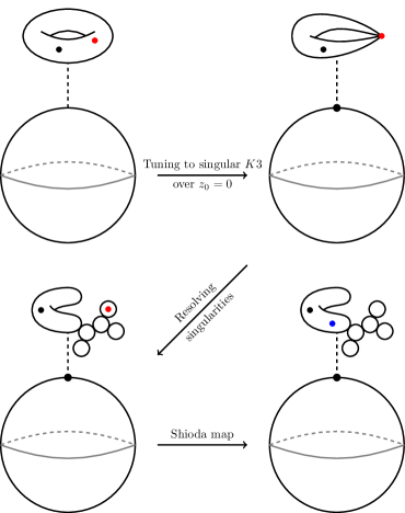
Figure 4: The fibration of the torus $\mathcal{E}$ over $\mathbb{P}^{1}$ (top left) turns via tuning into a singular $K3$ manifold (top right). Resolution of the singularity generates five $\mathbb{P}^{1}$s with SO(10) intersections (bottom left); after the Shioda map has been carried out, the U(1) divisor intersects the affine node $\mathbb{P}^{1}_{0}$ (bottom right).

The construction of a smooth CY twofold described in this section is summarized in Figure 4: the fibration of a torus with two points over a $\mathbb{P}^{1}$ yields a $K3$ manifold that can be tuned to have a codimension-one singularity corresponding to the group SO(10). Adding an SO(10) top to the fibered ambient space this singularity is resolved, leading to a smooth $K3$ manifold. The new fiber consists of the torus and five additional $\mathbb{P}^{1}$s which represent the resolution of the singularity. Finally, the Shioda map orthogonalizes the U(1) factor with respect to the SO(10) Cartan divisors.

2.3 Matter splits

In the following we investigate the codimension-two singularities in the fiber, which occur at the four loci listed in Table 3. Here the SO(10) symmetry enhances to SO(12) or E₆. One or more $\mathbb{P}^{1}$s of the fiber split into several $\mathbb{P}^{1}$s whose intersections correspond to the extended Dynkin diagram of the enhanced symmetry.

SO(12) matter locus $\mathbf{d_{9}=0}$

At this locus the equation for the curve $\mathbb{P}^{1}_{0}$ in Table 5 changes. The polynomial representing the CY twofold factorizes into three terms which means that $\mathbb{P}^{1}_{0}$ splits into three curves:

$$\begin{array}[]{c|ll }\text{nodes}&&\text{nodes after split}\\ \hline\cr\mathbb{P}^{1}_{0}&\rightarrow&z_{0}\cap(d_{5}ue_{1}+d_{8}g_{1}f_{3})+z_{0}\cap f_{2}+z_{0}\cap u\\ &&\equiv\mathbb{P}^{1}_{0a}+\mathbb{P}^{1}_{0,2}+\mathbb{P}^{1}_{0,u}\\ \mathbb{P}^{1}_{1}&&f_{2}\cap(d_{7}z_{0})\\ \mathbb{P}^{1}_{2}&&g_{1}\cap(d_{7}z_{0}f_{3}+d_{5}f_{2}f_{4})\\ \mathbb{P}^{1}_{3}&&g_{2}\cap(d_{1}g_{1}f_{4}+d_{3}v^{2}g_{1}f_{3}+d_{5}wf_{4}+d_{7}v^{2}wf_{3})\\ \mathbb{P}^{1}_{4}&&f_{3}\cap(d_{1}z_{0}g_{1}+d_{5}w)\\ \mathbb{P}^{1}_{5}&&f_{4}\cap(d_{3}uf_{2}g_{1}+d_{4}f_{2}g_{1}^{2}g_{2}+d_{7}w)\\ \hline\cr\end{array}$$ (2.59)

The other five $\mathbb{P}^{1}$s are not affected. One easily verifies that the new curves are again $\mathbb{P}^{1}$s by calculating the corresponding self-intersection numbers:

$$\begin{split}\mathbb{P}^{1}_{0a}:&\quad[z_{0}]\cdot[ue_{1}]\cdot([z_{0}]-[f_{2}]-[u])=-2\,,\\ \mathbb{P}^{1}_{0,2}:&\quad[z_{0}]\cdot[f_{2}]\cdot([z_{0}]-[ue_{1}]-[u])=-2\,,\\ \mathbb{P}^{1}_{0,u}:&\quad[z_{0}]\cdot[u]\cdot([z_{0}]-[ue_{1}]-[f_{2}])=-2\,,\end{split}$$ (2.60)

where the split of the original $\mathbb{P}^{1}_{0}$ has been taken into account in the last divisor. One of the split $\mathbb{P}^{1}_{0}$s is identical to one of the SO(10) $\mathbb{P}^{1}_{i}$s,

$$\mathbb{P}^{1}_{0,2}=\mathbb{P}^{1}_{2}\,,$$ (2.61)

$\mathbb{P}^{1}_{0,u}$ intersects with the exceptional torus divisor,

$$[e_{1}]\cdot\mathbb{P}^{1}_{0,u}=1\,,$$ (2.62)

whereas

$$[e_{1}]\cdot\mathbb{P}^{1}_{0a}=[e_{1}]\cdot\mathbb{P}^{1}_{0,2}=0\,.$$ (2.63)

Hence, $\mathbb{P}^{1}_{0,u}$ is the new affine node. The intersections of the new $\mathbb{P}_{0}^{1}$s are

$$\begin{split}\mathbb{P}^{1}_{0,u}\cap\mathbb{P}^{1}_{0,2}:&\quad[z_{0}]\cdot[u]\cdot[f_{2}]=1\,,\\ \mathbb{P}^{1}_{0,u}\cap\mathbb{P}^{1}_{0a}:&\quad[z_{0}]\cdot[ue_{1}]\cdot[u]=0\,,\\ \mathbb{P}^{1}_{0a}\cap\mathbb{P}^{1}_{0,2}:&\quad[z_{0}]\cdot[ue_{1}]\cdot[f_{2}]=1\,.\end{split}$$ (2.64)

Together with the SO(10) $\mathbb{P}^{1}$s one obtains the extended Dynkin diagram of SO(12) (see Figure 5).

Figure 5: Extended Dynkin diagram of SO(12) at the $d_{9}=0$ locus. The affine node has an intersection with $[e_{1}]$. The dashed circles indicate SO(10) nodes before the matter split.

The curve $\mathbb{P}^{1}_{0a}$ extends the Dynkin diagram of SO(10) to the Dynkin diagram of SO(12). $\mathbb{P}^{1}_{0a}$ can be identified as matter curve,

$$\mathbb{P}^{1}_{0a}=\mathcal{C}^{\omega}_{q}\,,$$ (2.65)

with Dynkin label and U(1) charge,

$$D_{i}\cdot\mathbb{P}^{1}_{0a}=\omega_{i}=(1,0,0,0,0)_{i}\,,\quad q=\sigma(\hat{s}_{i})\cdot\mathbb{P}^{1}_{0a}=3/2\,,$$ (2.66)

corresponding to a ${\bf 10}$-plet of SO(10). Since $\omega$ is the highest weight of the ${\bf 10}$ representation, all states can be obtained by adding SO(10) $\mathbb{P}^{1}_{i}$s, $i=1\ldots 5$ to $\mathbb{P}^{1}_{0a}$, which corresponds to the subtraction of roots $\alpha_{i}$ from $\omega$ in the usual way.

E₆ matter locus $\mathbf{d_{5}=0}$

At this locus the curves $\mathbb{P}^{1}_{0}$, $\mathbb{P}^{1}_{2}$ and $\mathbb{P}^{1}_{4}$ split into two $\mathbb{P}^{1}$s each:

$$\begin{array}[]{c|ll }\text{nodes}&&\text{nodes after split}\\ \hline\cr\mathbb{P}^{1}_{0}&\rightarrow&z_{0}\cap(d_{8}uf_{2}g_{1}+d_{9}v)+z_{0}\cap f_{3}\\ &&\equiv\mathbb{P}^{1}_{0a}+\mathbb{P}^{1}_{0,4}\\ \mathbb{P}^{1}_{1}&&f_{2}\cap(d_{7}z_{0}+d_{9}f_{4})\\ \mathbb{P}^{1}_{2}&\rightarrow&g_{1}\cap(d_{7}z_{0}+d_{9}g_{2}f_{4})+g_{1}\cap f_{3}\\ &&\equiv\mathbb{P}^{1}_{2a}+\mathbb{P}^{1}_{2,4}\\ \mathbb{P}^{1}_{3}&&g_{2}\cap(d_{1}g_{1}f_{4}+d_{3}g_{1}f_{3}+d_{7}wf_{3})\\ \mathbb{P}^{1}_{4}&\rightarrow&f_{3}\cap z_{0}+f_{3}\cap g_{1}\\ &&\equiv\mathbb{P}^{1}_{0,4}+\mathbb{P}^{1}_{2,4}\\ \mathbb{P}^{1}_{5}&&f_{4}\cap(d_{3}uf_{2}g_{1}+d_{4}f_{2}g_{1}^{2}g_{2}+d_{7}w)\\ \hline\cr\end{array}$$ (2.77)

Figure 6: Extended Dynkin diagram of E₆ at the $d_{5}=0$ locus. The affine node intersects $[e_{1}]$. The dashed ellipses indicate SO(10) nodes before the matter split. Two of the E₆ nodes occur in the split of two SO(10) nodes.

The curve $\mathbb{P}^{1}_{0a}$ is the only node which has nonvanishing intersection with $[e_{1}]$ and it therefore represents the new affine node. The four new nodes all have nonvanishing U(1) charge and the identification of the matter curve is unique up to complex conjugation and the addition of SO(10) roots. We choose

$$\mathbb{P}^{1}_{0,4}=\mathcal{C}^{\omega}_{q}\,,$$ (2.78)

with Dynkin label and U(1) charge

$$\quad D_{i}\cdot\mathbb{P}^{1}_{0,4}=\omega_{i}=(0,1,0,-1,0)_{i}\,,\quad q=\sigma(\hat{s}_{1})\cdot\mathbb{P}^{1}_{0,4}=3/4\,,$$ (2.79)

corresponding to a ${\bf 16}$-plet of SO(10). The remaining new $\mathbb{P}^{1}$s can then be written as linear combinations of the matter curve and SO(10) roots,

$$\begin{split}\mathbb{P}^{1}_{0a}&=-\mathcal{C}^{\omega}_{3/4}+\mathbb{P}^{1}_{0}\,,\\ \mathbb{P}^{1}_{2a}&=\mathcal{C}^{\omega}_{3/4}-\mathbb{P}^{1}_{4}+\mathbb{P}^{1}_{2}\,,\\ \mathbb{P}^{1}_{2,4}&=-\mathcal{C}^{\omega}_{3/4}+\mathbb{P}^{1}_{4}\,.\end{split}$$ (2.80)

It is straightforward to calculate the intersections of the curves given in (2.77). As a result one obtains the extended Dynkin diagram of E₆ (see Figure 6).

E₆ matter locus $\mathbf{d_{7}=0}$

Here again an enhancement from SO(10) to E₆ takes place. This time the curves $\mathbb{P}^{1}_{2}$ and $\mathbb{P}^{1}_{5}$ split into two and three $\mathbb{P}^{1}$s, respectively:

$$\begin{array}[]{c|ll }\text{nodes}&&\text{nodes after split}\\ \hline\cr\mathbb{P}^{1}_{0}&&z_{0}\cap(d_{5}u^{2}e_{1}f_{2}+d_{8}uf_{2}g_{1}f_{3}+d_{9}vf_{3})\\ \mathbb{P}^{1}_{1}&&f_{2}\cap f_{4}\equiv\mathbb{P}^{1}_{1,5}\\ \mathbb{P}^{1}_{2}&\rightarrow&g_{1}\cap(d_{5}f_{2}+d_{9}g_{2}f_{3})+g_{1}\cap f_{4}\\ &&\equiv\mathbb{P}^{1}_{2a}+\mathbb{P}^{1}_{2,5}\\ \mathbb{P}^{1}_{3}&&g_{2}\cap(d_{1}g_{1}f_{4}+d_{3}g_{1}f_{3}+d_{5}wf_{4})\\ \mathbb{P}^{1}_{4}&&f_{3}\cap(d_{1}z_{0}g_{1}+d_{5}w)\\ \mathbb{P}^{1}_{5}&\rightarrow&f_{4}\cap(d_{3}u+d_{4}g_{1}g_{2})+f_{4}\cap f_{2}+f_{4}\cap g_{1}\\ &&\equiv\mathbb{P}^{1}_{5a}+\mathbb{P}^{1}_{1,5}+\mathbb{P}^{1}_{2,5}\\ \hline\cr\end{array}$$ (2.90)

Figure 7: Extended Dynkin diagram of E₆ at the $d_{7}=0$ locus. The affine node has an intersection with $[e_{1}]$. The dashed ellipses indicate SO(10) nodes before the matter split.

The affine node $\mathbb{P}^{1}_{0}$ is unaffected by the splits. The identification of the matter curve is again unique up to complex conjugation and addition of roots. We choose

$$\mathbb{P}^{1}_{2a}=\mathcal{C}^{\omega}_{q}\,,$$ (2.91)

with Dynkin label and U(1) charge

$$D_{i}\cdot\mathbb{P}^{1}_{2a}=\omega_{i}=(0,-1,0,0,1)_{i}\,,\quad q=\sigma(\hat{s_{1}})\cdot\mathbb{P}^{1}_{2a}=-1/4\,,$$ (2.92)

corresponding again to a ${\bf 16}$-plet of SO(10). The other two new roots are linear combinations of the matter curve and SO(10) $\mathbb{P}^{1}$s,

$$\mathbb{P}^{1}_{2,5} =-\mathcal{C}^{\omega}_{-1/4}+\mathbb{P}^{1}_{2}\,,$$ (2.93)

$$\mathbb{P}^{1}_{5a} =\mathcal{C}^{\omega}_{-1/4}-\mathbb{P}^{1}_{1}-\mathbb{P}^{1}_{2}+\mathbb{P}^{1}_{5}\,.$$ (2.94)

Calculating the intersection numbers of all $\mathbb{P}^{1}$s one finds again the extended Dynkin diagram of E₆. This is displayed in Figure 7 where also the split of the SO(10) $\mathbb{P}^{1}$s is indicated by dashed ellipses.

SO(12) matter locus $\mathbf{d_{3}d_{5}-d_{1}d_{7}=0}$

Finally, at this locus a second enhancement of SO(10) to SO(12) occurs. In this case only $\mathbb{P}^{1}_{3}$ splits into two $\mathbb{P}^{1}$s:

$$\begin{array}[]{c|ll }\text{nodes}&&\text{nodes after split}\\ \hline\cr\mathbb{P}^{1}_{0}&&z_{0}\cap(d_{5}u^{2}e_{1}f_{2}+d_{8}uf_{2}g_{1}f_{3}+d_{9}vf_{3})\\ \mathbb{P}^{1}_{1}&&f_{2}\cap(d_{7}z_{0}+d_{9}f_{4})\\ \mathbb{P}^{1}_{2}&&g_{1}\cap(d_{5}f_{2}f_{4}+d_{7}z_{0}f_{3}+d_{9}g_{2}f_{3}f_{4})\\ \mathbb{P}^{1}_{3}&\rightarrow&g_{2}\cap(d_{1}g_{1}+d_{5}w)+g_{2}\cap(d_{1}f_{4}+d_{3}f_{3})\\ &&\equiv\mathbb{P}^{1}_{3a}+\mathbb{P}^{1}_{3b}\\ \mathbb{P}^{1}_{4}&&f_{3}\cap(d_{1}z_{0}g_{1}+d_{5}w)\\ \mathbb{P}^{1}_{5}&&f_{4}\cap(d_{3}uf_{2}g_{1}+d_{4}f_{2}g_{1}^{2}g_{2}+d_{7}w)\\ \hline\cr\end{array}$$ (2.103)

Figure 8: Extended Dynkin diagram of SO(12) at the $d_{3}d_{5}-d_{1}d_{7}=0$ locus. The affine node intersects with $[e_{1}]$. The dashed ellipse indicates the SO(10) node $\mathbb{P}^{1}_{3}$.

One immediately identifies, up to complex conjugation, the matter curve

$$\mathbb{P}^{1}_{3a}=\mathcal{C}^{\omega}_{q}\,,$$ (2.104)

with Dynkin label and U(1) charge

$$\quad D_{i}\cdot\mathbb{P}^{1}_{3a}=\omega_{i}=(0,1,-1,0,0)_{i}\,,\quad q=\sigma(\hat{s}_{1})\cdot\mathbb{P}^{1}_{3a}=-1/2\,,$$ (2.105)

corresponding to a ${\bf 10}$-plet of SO(10). The second new $\mathbb{P}^{1}$ is given by

$$\mathbb{P}^{1}_{3b}=-\mathcal{C}^{\omega}_{-1/2}+\mathbb{P}^{1}_{3}\,.$$ (2.106)

The intersection number of all $\mathbb{P}^{1}$s yield the Dynkin diagram displayed in Figure 8.

The symmetry enhancements and matter representations at all four matter loci are summarized in Table 6.

$\begin{array}[]{| c | c | c | c |}\hline\cr\text{locus}&\text{Ord}(f,g,\Delta)&\text{fiber singularity}&\text{representation}\\ \hline\cr\hline\cr z_{0}=d_{9}=0&(2,3,8)&$SO$(12)&\mathbf{10}_{3/2}\\ \hline\cr z_{0}=d_{5}=0&(3,4,8)&$E$_{6}&\mathbf{16}_{3/4}\\ \hline\cr z_{0}=d_{7}=0&(3,4,8)&$E$_{6}&\mathbf{16}_{-1/4}\\ \hline\cr z_{0}=d_{3}d_{5}-d_{1}d_{7}=0&(2,3,8)&$SO$(12)&\mathbf{10}_{-1/2}\\ \hline\cr\end{array}$

Table 6: Codimension-two loci, enhanced symmetry groups and matter representations.

2.4 Yukawa couplings of SO(10) matter

For completeness, we now consider Yukawa couplings of SO(10) matter. Tuning two coefficients of the polynomial (2.26) to zero, one finds further symmetry enhancements corresponding to codimension-three singularities of a CY fourfold. At these loci three matter curves intersect and Yukawa couplings are generated.

Let us first consider the locus $z_{0}=d_{5}=d_{7}=0$, where also $d_{1}d_{7}-d_{3}d_{5}=0$. According to Table 6 at this locus three matter curves intersect, which leads to the Yukawa coupling $\mathbf{16}_{3/4}\mathbf{16}_{-1/4}\mathbf{10}_{-1/2}$. It is instructive to study the matter splits, starting from (2.77) or (2.90). The result reads:

$$\begin{array}[]{c|ll }\text{nodes}&&\text{nodes after split}\\ \hline\cr\mathbb{P}^{1}_{0}&\rightarrow&z_{0}\cap(d_{8}uf_{2}g_{1}+d_{9}v)+z_{0}\cap f_{3}\equiv\mathbb{P}^{1}_{0a}+\mathbb{P}^{1}_{0,4}\\ \mathbb{P}^{1}_{1}&\rightarrow&f_{2}\cap f_{4}\equiv\mathbb{P}^{1}_{1,5}\\ \mathbb{P}^{1}_{2}&\rightarrow&g_{1}\cap g_{2}+g_{1}\cap f_{3}+g_{1}\cap f_{4}\equiv\mathbb{P}^{1}_{2,3}+\mathbb{P}^{1}_{2,4}+\mathbb{P}^{1}_{2,5}\\ \mathbb{P}^{1}_{3}&\rightarrow&g_{2}\cap g_{1}+g_{2}\cap(d_{1}f_{4}+d_{3}f_{3})\equiv\mathbb{P}^{1}_{2,3}+\mathbb{P}^{1}_{3b}\\ \mathbb{P}^{1}_{4}&\rightarrow&f_{3}\cap z_{0}+f_{3}\cap g_{1}\equiv\mathbb{P}^{1}_{0,4}+\mathbb{P}^{1}_{2,4}\\ \mathbb{P}^{1}_{5}&\rightarrow&f_{4}\cap(d_{3}u+d_{4}g_{1}g_{2})+f_{4}\cap f_{2}+f_{4}\cap g_{1}\equiv\mathbb{P}^{1}_{5a}+\mathbb{P}^{1}_{1,5}+\mathbb{P}^{1}_{2,5}\\ \hline\cr\end{array}$$ (2.114)

Now all six SO(10) $\mathbb{P}^{1}$s split, yielding eight $\mathbb{P}^{1}$s some of which occur twice. These $\mathbb{P}^{1}$s provide links between the chains of $\mathbb{P}^{1}$s into which the original SO(10) $\mathbb{P}^{1}$s split. These links determine the intersection pattern of all $\mathbb{P}^{1}$s and as a result one easily obtains the extended Dynkin diagram of $\text{E}_{7}$ shown in Figure 9. The affine node is again indicated by the intersection with the divisor $[e_{1}]$, and the dashed ellipses indicate the SO(10) $\mathbb{P}^{1}$s before the matter splits.

Figure 9: Extended Dynkin diagram of E₇ at the locus $z_{0}=d_{5}=d_{7}=0$ with Yukawa coupling $\mathbf{16}_{3/4}\mathbf{16}_{-1/4}\mathbf{10}_{-1/2}$; the affine node intersects with $[e_{1}]$, the dashed ellipses indicate the SO(10) $\mathbb{P}^{1}$s before the matter splits.

At the locus $z_{0}=d_{9}=0$ we have chosen the representation $\mathbf{10}_{3/2}$ as matter curve. Alternatively, we could have chosen the complex conjugate representation $\mathbf{10}_{-3/2}$ as matter curve. In this case a Yukawa coupling $\mathbf{16}_{3/4}\mathbf{16}_{3/4}\mathbf{10}_{-3/2}$ can be generated at the locus $z_{0}=d_{5}=d_{9}=0$, where we find a non-Kodaira fiber. The intersections of the $\mathbb{P}^{1}$s are displayed in Figure 10, which is reminiscent of the extended E₇ Dynkin diagram, with a missing node in the middle. Such an intersection pattern has previously been observed in [63].

Figure 10: $\mathbb{P}^{1}$ intersection pattern at $z_{0}=d_{7}=d_{9}=0$; non-Kodaira singularity with Yukawa coupling $\mathbf{16}_{3/4}\mathbf{16}_{3/4}\mathbf{10}_{-3/2}$.

Anticipating $d_{8}=d_{9}=0$ as locus of singlets with charge three (see (3.10)), we note that at $z_{0}=d_{8}=d_{9}=0$ a Yukawa coupling $\mathbf{10}_{-3/2}\mathbf{10}_{-3/2}\mathbf{1}_{3}$ can be generated. We again find a codimension-three singularity that is not of Kodaira type. The intersection pattern of the $\mathbb{P}^{1}$s is shown in Figure 11. It represents the (non-affine) Dynkin diagram of SO(14). The torus divisor $[e_{1}]$ wraps the affine node entirely, corresponding to an intersection number $-1$, which is indicated by a striped circle. A similar pattern has previously been observed in [63].

Figure 11: $\mathbb{P}^{1}$ intersection pattern at $z_{0}=d_{8}=d_{9}$; non-Kodaira singularity with Yukawa coupling $\mathbf{10}_{-3/2}\mathbf{10}_{-3/2}\mathbf{1}_{3}$

Finally, at the locus $z_{0}=d_{3}d_{5}-d_{1}d_{7}=d_{7}=0$ we find the intersection pattern of $\mathbb{P}^{1}$s shown in Figure 12, which is the non-affine Dynkin diagram of $\text{E}_{7}$. The corresponding Yukawa coupling is $\mathbf{16}_{-1/4}\mathbf{16}_{-1/4}\mathbf{10}_{1/2}$.

Figure 12: $\mathbb{P}^{1}$ intersection pattern at $z_{0}=d_{3}d_{5}-d_{1}d_{7}=d_{7}=0$; non-Kodaira singularity with Yukawa coupling $\mathbf{16}_{-1/4}\mathbf{16}_{-1/4}\mathbf{10}_{1/2}$

2.5 Calabi-Yau threefold and matter multiplicities

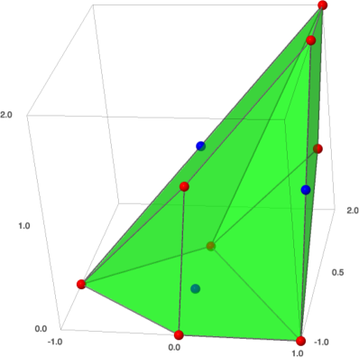
Figure 13: The polytope formed by $F_{3}$ and an SO(10) top with vertices listed in the table. The polygon $F_{3}$ is visible at height $0$; four SO(10) vertices appear at height $1$ and the other two at height $2$. The vertices corresponding to $z_{1}$ and the coordinates $z_{2}$, $z_{3}$ of the second $\mathbb{P}^{1}$ are not shown in the figure.

So far we have analyzed the fibration of a torus over a $\mathbb{P}^{1}$ base space, which gave us the gauge group SO(10)$\times$U(1) and which allowed us, after tuning, to anticipate loci of matter and Yukawa couplings. These all lie in the hyperplane of the GUT divisor $\mathcal{Z}$, which is the projection of $[z_{0}]$ to the base, and are furthermore characterized by the vanishing of certain coefficients $d_{i}$ of the polynomial $p_{Y_{2}}$. The $d_{i}$ are polynomials in the base coordinates $z_{0}$ and $z_{1}$ (see (A.10)). The multiplicities of the matter fields are fixed once the twofold $Y_{2}$ is extended to a threefold $Y_{3}$. In the following we shall consider the simplest case which corresponds to adding a second $\mathbb{P}^{1}$ with coordinates $z_{2}$, $z_{3}$. The coefficients of the polynomials $d_{i}(z_{0},z_{1})$ then also depend on the additional coordinates $z_{2}$ and $z_{3}$.

For this specific case the full threefold geometry is given in Figure 13. The polytope is defined in a four-dimensional lattice $\mathbb{Z}^{4}$ with vertices $v_{i}=(v_{i}^{1},\dots,v_{i}^{4})$. A projection onto the two-dimensional base space can be obtained by projecting onto the last two coordinates,

$$(v_{i}^{1},v_{i}^{2},v_{i}^{3},v_{i}^{4})\xrightarrow[]{\pi}(v_{i}^{3},v_{i}^{4})\,.$$ (2.115)

The base coordinates now correspond to vertices in a $\mathbb{Z}^{2}$ lattice, $z_{0}:(1,0)$, $z_{1}:(-1,0)$, $z_{2}:(0,1)$, $z_{3}:(0,-1)$, which form the toric diagram of $\mathbb{P}^{1}\times\mathbb{P}^{1}=\mathbb{F}_{0}$. This base space has two divisor classes,

$$\mathcal{Z}\sim\pi_{B}([z_{0}])\equiv H_{1}\,,\quad[z_{2}]\sim[z_{3}]\equiv H_{2}\,,$$ (2.116)

with the intersection numbers

$$H_{1}^{2}=H_{2}^{2}=0\,,\quad H_{1}\cdot H_{2}=1\ .$$ (2.117)

From the dependence of the coefficients $d_{i}$ on the base coordinates (see Eq. (A.13)) one can read off the relations between the divisors $[d_{i}]$ and the base divisors $H_{1}$ and $H_{2}$. The divisors $[d_{i}]$ are effective, i.e. they are linear combinations of $H_{1}$ and $H_{2}$ with positive coefficients,

$$\begin{array}[]{llll}&[d_{1}]\sim 0\,,&[d_{2}]\sim 2H_{2}\,,&[d_{3}]\sim H_{1}+4H_{2}\,,\\ &[d_{4}]\sim H_{1}+6H_{2}\,,&[d_{5}]\sim H_{1}\,,&[d_{6}]\sim H_{1}+2H_{2}\,,\\ &[d_{7}]\sim 2H_{1}+4H_{2}\,,&[d_{8}]\sim H_{1}&[d_{9}]\sim 2H_{1}+2H_{2}\,.\end{array}$$ (2.121)

Given the intersection numbers (2.117) one can also easily calculate the genus of the GUT divisor $\mathcal{Z}$,

$$g =1-\genfrac{}{}{}{1}{1}{2}([K_{B}^{-1}]-\mathcal{Z})\cdot\mathcal{Z}$$

$$=1-\genfrac{}{}{}{1}{1}{2}(2H_{1}+2H_{2}-H_{1})H_{1}=0\,,$$ (2.122)

where we have used that the anticanonical divisor is given by $[K_{B}^{-1}]=2H_{1}+2H_{2}$. It is no surprise that the GUT divisor $\mathcal{Z}$ is a genus-zero curve since it was just a point on the one-dimensional base $\mathbb{P}^{1}$ of $K3$. It is an immediate consequence that the considered model has no matter multiplets in the adjoint representation of SO(10).

Intersections of the GUT divisor with the four matter loci yield the multiplicities of matter representations. For instance, for the $\mathbf{10}$-plet at $z=d_{9}=0$, one has (cf. (2.121))

$$n[\mathbf{10}_{3/2}]=[d_{9}]\cdot\mathcal{Z}=(2H_{1}+2H_{2})\cdot H_{1}=2\,.$$ (2.123)

For the other SO(10) representations, and the charged and neutral singlets one finds:

$$\begin{array}[]{c|c|c}\text{representation}&\text{locus}&\text{multiplicity}\\ \hline\cr\mathbf{10}_{3/2}&z=d_{9}=0&2\\ \mathbf{16}_{3/4}&z=d_{5}=0&0\\ \mathbf{16}_{-1/4}&z=d_{7}=0&4\\ \mathbf{10}_{-1/2}&z=0=d_{3}d_{5}-d_{1}d_{7}&4\\ \hline\cr\mathbf{45}&z=0&0\\ \hline\cr\mathbf{1}_{1}&V(I_{3})&2\\ \mathbf{1}_{2}&V(I_{2})&36\\ \mathbf{1}_{3}&V(I_{1})&76\\ \mathbf{1}_{0}&&51+1\\ T&&1\\ \hline\cr\end{array}$$ (2.135)

A detailed, base-independent discussion of the singlet multiplicities will be given in Section 3.

SO(10) gauge fields live in a space of real dimension eight, defined by a GUT divisor of codimension one. Similarly, SO(10) matter is located in a six-dimensional subspace defined by the intersection of two divisors. Once we extend the CY threefold considered so far to a CY fourfold, the matter points become matter curves which can intersect in the compact dimensions, leading to the generation of Yukawa couplings. For the considered model this generic pattern is illustrated in Figure 14.

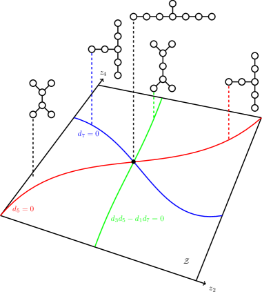
Figure 14: In a complex three-dimensional space, SO(10) matter is represented by curves in the plane $\mathcal{Z}$, the locus of the SO(10) gauge fields. The curves of the matter fields ${\bf 16}_{3/4}$ ($z_{0}=d_{5}=0$), ${\bf 16}_{-1/4}$ ($z_{0}=d_{7}=0$) and ${\bf 10}_{-1/2}$ ($z_{0}=d_{1}d_{7}-d_{3}d_{5}=0$) intersect at the codimension-three E₇ singularity $z_{0}=d_{5}=d_{7}=d_{1}d_{7}-d_{3}d_{5}=0$.

2.6 Anomaly cancellation

With the matter spectrum at hand we can check the vanishing of the irreducible anomalies as well as the factorization of the remaining anomaly polynomial $\mathcal{I}_{8}$. We compute the neutral singlets in (2.135) from the Euler and Hodge numbers of the threefold,

$$(h^{1,1},h^{2,1})_{\chi}=(9,51)_{-84}\,,$$ (2.136)

which we evaluated using SAGE and which coincides with the general formula given in Appendix C. As expected, the nine Kähler deformations come from the six Cartan generators of the gauge group, one from the torus and two from the base.

The theory contains $V=46$ vector multiplets accounting for the gauge fields of the group SO(10)$\times$U(1), $H=290$ hypermultiplets from the charged and uncharged fields in (2.135), and a single tensor multiplet, $T=1$. The irreducible gravitational part of the anomaly polynomial then reads

$$\begin{split}\mathcal{I}_{8}\supset&-\frac{1}{5760}(H-V+29T-273)\left(\text{tr}R^{4}+\genfrac{}{}{}{1}{5}{4}(\text{tr}R^{2})^{2}\right)\\ =&-\frac{1}{5760}(290-46+29-273)\left(\text{tr}R^{4}+\genfrac{}{}{}{1}{5}{4}(\text{tr}R^{2})^{2}\right)=0\,,\end{split}$$ (2.137)

i.e., it vanishes for the given field content.

Similarly, we can evaluate the irreducible non-Abelian part of the anomaly polynomial. Rewriting the traces of adjoint representation, Tr, and spinor representation, $\text{tr}_{\mathbf{16}}$, in terms of $\text{tr}_{\mathbf{10}}\equiv\text{tr}$,

$$\begin{split}\operatorname{\text{tr}}_{\mathbf{16}}\tilde{F}^{2}&=2\,\operatorname{\text{tr}}\tilde{F}^{2}\,,\quad\operatorname{\text{tr}}_{\mathbf{16}}\tilde{F}^{4}=-\operatorname{\text{tr}}\tilde{F}^{4}+\genfrac{}{}{}{1}{3}{4}(\operatorname{\text{tr}}\tilde{F}^{2})^{2}\,,\\ \text{Tr}\tilde{F}^{2}&=8\,\operatorname{\text{tr}}\tilde{F}^{2}\,,\quad\text{Tr}\tilde{F}^{4}=2\operatorname{\text{tr}}\tilde{F}^{4}+3(\operatorname{\text{tr}}\tilde{F}^{2})^{2}\,,\end{split}$$ (2.138)

we find

$$\begin{split}\mathcal{I}_{8}&\supset\frac{1}{24}\left(\text{Tr}\tilde{F}^{4}-4\,\text{tr}_{16}\tilde{F}^{4}-6\,\text{tr}\tilde{F}^{4}\right)\\ &=\frac{1}{24}(2+4-6)\,\text{tr}\tilde{F}^{4}+\frac{1}{24}(3-3)(\text{tr}\tilde{F}^{2})^{2}=0\,,\end{split}$$ (2.139)

where $\tilde{F}$ denotes the SO(10) field strength. We see that for the given matter spectrum even the reducible part vanishes. The remaining contributions to the anomaly polynomial evaluated with the spectrum (2.135) are

$$\mathcal{I}_{8}=-\frac{1}{16}(\text{tr}R^{2})^{2}+\frac{1}{16}\text{tr}R^{2}\,\text{tr}\,\tilde{F}^{2}+\frac{99}{32}\text{tr}R^{2}\,F^{2}-\frac{3}{2}\text{tr}\tilde{F}^{2}\,F^{2}-\frac{153}{4}F^{4}\,,$$ (2.140)

with U(1) field strength $F$. This anomaly polynomial factorizes,

$$\mathcal{I}_{8}=-\frac{1}{16}\left(\text{tr}R^{2}-\text{tr}\tilde{F}^{2}-\genfrac{}{}{}{1}{51}{2}F^{2}\right)\left(\text{tr}R^{2}-24F^{2}\right)\,.$$ (2.141)

In the conventions of [67] and Section 4.3 this corresponds to the anomaly coefficients

$$a=\begin{pmatrix}2\\ 2\end{pmatrix}\,,\quad b=\begin{pmatrix}-1\\ 0\end{pmatrix}\,,\quad b_{11}=\begin{pmatrix}-\genfrac{}{}{}{1}{51}{4}\\ -12\end{pmatrix}\,,$$ (2.142)

which match the expressions derived from the general approach in Section 4.3.

3 Base-independent matter multiplicities

In this section we extend the discussion for the specific base $B=\mathbb{F}_{0}$ given above to a general base space. This allows us to derive base-independent expressions for the matter multiplicities.

3.1 Counting singlets

In Section 2.2 we have discussed codimension-two singularities where the GUT symmetry SO(10) is enhanced to SO(12) or E₆ and where matter multiplets are localized with quantum numbers in the coset of SO(12)/SO(10) and E₆/SO(10), respectively. However, already the torus fibration $\mathcal{E}$ admits SU(2) singularities where SO(10) singlets occur as matter fields with U(1) charge. Once the torus is fibered over a two-dimensional base these singularities correspond to the loci of matter multiplets. For the tori corresponding to the $16$ ambient spaces, codimension-two singularities have been comprehensively analyzed in [49] and the U(1) charges of the matter fields have been determined. Adding an SO(10) top does not change the U(1) charges of the SO(10) singlet fields but it does affect their multiplicities, which we shall study in this section.

Let us recall how one finds the loci of charged matter fields in the case without an SO(10) top, following the discussion in [49]. In a first step one has to rewrite the torus in Weierstrass form. The elliptic curve obtained from $F_{3}$ has one rational point with coordinates $(x_{1},y_{1},z_{1})$. In this case the Weierstrass form can be written as [54]

$$F =-y^{2}+x^{3}+fx+g=0\,,$$

$$f =c-\hat{x}_{1}^{2}\,,\quad g=-c\hat{x}_{1}-\hat{y}_{1}^{2}\,.$$ (3.1)

Here $c$ is a constant and we have used a $\mathbb{C}^{*}$-action, $(x,y,z)\rightarrow(\hat{x},\hat{y},1)=(x/z^{2},y/z^{3},1)$, such that the coordinates of the rational point are $(\hat{x}_{1},\hat{y}_{1},1)$. A singular point $(x,y)$, with

$$F=\frac{\partial F}{\partial x}=\frac{\partial F}{\partial y}=0\,,$$

occurs if the discriminant

$$\Delta =4f^{3}+27g^{2}$$

$$=(4c-\hat{x}_{1}^{2})(c+2\hat{x}_{1}^{2})^{2}+54\hat{y}_{1}^{2}c\hat{x}_{1}+27\hat{y}_{1}^{4}$$ (3.2)

vanishes. This happens for

$$\hat{y}_{1}=c+2\hat{x}_{1}^{2}=0$$ (3.3)

at $(\hat{x},\hat{y})=(\hat{x}_{1},0)$. From Eqs. (3.1) and (3.1) we infer that at this point the torus has an $\text{Ord}(f,g,\Delta)=(0,0,2)$ singularity associated with the group SU(2). As expected we have a codimension-two singularity as in the case of the matter loci discussed in Section 2.2.

For a fibration of the torus over a two-dimensional base the two conditions (3.3) define matter curves. Replacing $c$ by the function $f$ (see Eq. (3.1)), and going back to homogeneous coordinates, the two conditions can be written as

$$y_{1}=z_{1}^{4}f+3x_{1}^{2}=0\,.$$ (3.4)

The coordinates $x_{1}$, $y_{1}$, $z_{1}$ and $f$ are known functions of the coefficients $s_{1},\ldots,s_{9}$ [49]. The conditions (3.4) imply that two polynomials, $P_{1}(s_{i})$ and $P_{2}(s_{i})$, vanish. To find the corresponding roots it is helpful to consider $P_{1}$ and $P_{2}$ as generators of a codimension-two ideal and to decompose this into irreducible prime ideals. One finds three prime ideals, $I_{1}$, $I_{2}$ and $I_{3}$ whose zeros correspond to the loci $V(I_{1})$, $V(I_{2})$ and $V(I_{3})$ of singlets with charge $3$, $2$ and $1$, respectively. For the loci corresponding to the prime ideals $I_{1}$ and $I_{2}$ one obtains [49]:

$$\begin{array}[]{c|l}\text{singlet}&\qquad\qquad\text{constraint}\\ \hline\cr\mathbf{1}_{3}&V(I_{1}):s_{8}=s_{9}=0\\ \mathbf{1}_{2}&V(I_{2}):s_{4}s_{8}^{3}-s_{3}s_{8}^{2}s_{9}+s_{2}s_{8}s_{9}^{2}-s_{1}s_{9}^{3}\\ &\qquad\qquad=s_{7}s_{8}^{2}+s_{5}s_{9}^{2}-s_{6}s_{8}s_{9}=0\\ &\qquad\qquad(s_{8},s_{9})\neq(0,0)\end{array}$$ (3.10)

Since the generators of the prime ideal $I_{3}$ are polynomials of high order, the determination of the corresponding zeros is technically nontrivial. This problem will be solved in the next section by unhiggsing the SO(10)$\times$U(1) fiber to an $\text{SO(10)$\times$U(1)}^{2}$ fiber.

In order to count the number of charge-two singlets one has to determine how often the ideal $I_{1}$ is contained in $I_{2}$. This can be done by means of the resultant technique [68]. For the two polynomials $Q_{1}(s_{8},s_{9})$ and $Q_{2}(s_{8},s_{9})$ of the ideal $I_{2}$ (see (3.10)) one defines the resultant with respect to $s_{8}$,

$$R=\textit{Res}_{s_{8}}(Q_{1},Q_{2})\,,$$ (3.11)

which is a polynomial in $s_{9}$. The resultant has the property that for every root $s_{9}=\beta$ of $R$ there exists a value $s_{8}=\alpha$ with $Q_{1}(\alpha,\beta)=Q_{2}(\alpha,\beta)=0$. The explicit expression for the resultant reads

$$\begin{split}R=&s_{9}^{6}(s_{4}^{2}s_{5}^{3}-s_{3}s_{4}s_{5}^{2}s_{6}+s_{2}s_{4}s_{5}s_{6}^{2}-s_{1}s_{4}s_{6}^{3}+s_{3}^{2}s_{5}^{2}s_{7}-2s_{2}s_{4}s_{5}^{2}s_{7}-s_{2}s_{3}s_{5}s_{6}s_{7}\\ &+3s_{1}s_{4}s_{5}s_{6}s_{7}+s_{1}s_{3}s_{6}^{2}s_{7}+s_{2}^{2}s_{5}s_{7}^{2}-2s_{1}s_{3}s_{5}s_{7}^{2}-s_{1}s_{2}s_{6}s_{7}^{2}+s_{1}^{2}s_{7}^{3})\,.\end{split}$$ (3.12)

Hence, $R$ has a root of order $6$ at $s_{9}=0$, with $Q_{1}(0,0)=Q_{2}(0,0)=0$. Correspondingly, the ideal $I_{1}$ is contained six times in the ideal $I_{2}$. The singlet multiplicities are determined by the intersection numbers of the base divisors. For the base $\mathbb{F}_{0}=\mathbb{P}^{1}\times\mathbb{P}^{1}$ of the previous section one finds $n[\mathbf{1}_{3}]=[s_{8}]\cdot[s_{9}]$, $n[\mathbf{1}_{2}]=[Q_{1}]\cdot[Q_{2}]-6[s_{8}]\cdot[s_{9}]$.

Adding the SO(10) top to the fiber changes the singlet multiplicities. As discussed in Section 2.2, the coefficients $s_{i}$ now depend on the base coordinates, $s_{i}=z_{0}^{n_{i}}d_{i}(z_{0},z_{1})$. This implies that the ideals (3.10) for the singlet localization are modified:

$$\begin{array}[]{c|l|c}\text{singlet}&\qquad\qquad\text{constraint}&\text{multiplicity}\\ \hline\cr\mathbf{1}_{3}&V(I_{1}):d_{8}=d_{9}=0&2\\ \mathbf{1}_{2}&V(I_{2}):d_{4}d_{8}^{3}z_{0}^{2}-d_{3}d_{8}^{2}d_{9}z_{0}+d_{2}d_{8}d_{9}^{2}z_{0}-d_{1}d_{9}^{3}\\ &\qquad\qquad=d_{7}d_{8}^{2}z_{0}+d_{5}d_{9}^{2}-d_{6}d_{8}d_{9}z_{0}=0\\ &\qquad\qquad(d_{8},d_{9})\neq 0,(z_{0},d_{5})\neq 0,(z_{0},d_{9})\neq 0&36\end{array}$$ (3.18)

Now the two polynomials $Q_{1}$ and $Q_{2}$ of the ideal $I_{2}$ also depend on $z_{0}$. Note that the two polynomials, after imposing the factorization, factor out powers of $z_{0}$ by which we have to divide, as this leads to unwanted solutions over $z_{0}=0$ where SO(10) charged multiplets are localized. In order to find the number of singlets with charge $q=2$, we have to subtract the number of solutions of $d_{8}=d_{9}=0$ as well as those of $z_{0}=d_{9}=0$, $z_{0}=d_{5}=0$, $z_{0}=d_{7}=0$ and $z_{0}=d_{3}d_{5}-d_{1}d_{7}=0$, which correspond to SO(10) matter (see Table 3). The evaluation of the resultant with respect to $z_{0}$ yields

$$\textit{Res}_{z_{0}}(Q_{1},Q_{2})=d_{8}^{2}d_{9}^{3}\hat{R}\,,$$ (3.19)

where $\hat{R}$ is a non-factorizable polynomial of degree five in the $d_{i}$. We conclude that the locus $z_{0}=d_{9}=0$ is contained three times in the ideal $I_{2}$.. Analogously, one can calculate the resultant with respect to $d_{9}$, which is given by

$$\textit{Res}_{d_{9}}(Q_{1},Q_{2})= d_{8}^{6}z_{0}^{3}(d_{3}^{2}d_{5}^{2}d_{7}-2d_{1}d_{3}d_{5}d_{7}^{2}+d_{1}^{2}d_{7}^{3}+d_{4}^{2}d_{5}^{3}z_{0}-d_{3}d_{4}d_{5}^{2}d_{6}z_{0}$$

$$-2d_{2}d_{4}d_{5}^{2}d_{7}z_{0}-d_{2}d_{3}d_{5}d_{6}d_{7}z_{0}+3d_{1}d_{4}d_{5}d_{6}d_{7}z_{0}+d_{1}d_{3}d_{6}^{2}d_{7}z_{0}$$

$$+d_{2}^{2}d_{5}d_{7}^{2}z_{0}-d_{1}d_{2}d_{6}d_{7}^{2}z_{0}+d_{2}d_{4}d_{5}d_{6}^{2}z_{0}^{2}-d_{1}d_{4}d_{6}^{3}z_{0}^{2})$$ (3.20)

The factor $d_{8}^{6}z_{0}^{3}$ implies one solution $d_{8}=d_{9}=0$ to order six, as in the case without SO(10) top, and a second solution $z_{0}=d_{9}=0$ to order three, which is consistent with the resultant (3.19). For the base $\mathbb{F}_{0}=\mathbb{P}^{1}\times\mathbb{P}^{1}$ the number of charge-two singlets is then given by

$$n[\mathbf{1}_{2}]=[Q_{1}]\cdot[Q_{2}]-6[d_{8}]\cdot[d_{9}]-3[z_{0}]\cdot[d_{9}]=36\,,$$ (3.21)

where we have used Eqs. (2.116) - (2.121).

3.2 Parametrizing the base dependence

So far we have expressed singlet multiplicities in terms of intersection numbers of the base divisors $[d_{i}]$ and $[z_{0}]$. In order to determine the multiplicities one has to specify a base and calculate the intersection numbers. A convenient parametrization of the base dependence has been given in [68, 59]. It has been used in the classification of all toric hypersurface fibrations [49], and we shall also use it in our analysis of all toric 6d F-theory vacua with SO(10) gauge symmetry.

The toric ambient space $X_{F_{3}}$ has four coordinates, $u$, $v$, $w$ and $e_{1}$, and the polynomial $p_{F_{3}}$ depends on nine coefficients $s_{1},\ldots s_{9}$. For a fibration over a two-dimensional base all these quantities become functions of the base coordinates. Equivalently, one can use the two sections $s_{7}$ and $s_{9}$ to parametrize the base dependence. Furthermore, by means of two $\mathbb{C}^{*}$-actions one can achieve that only two coordinates, $u$ and $v$, depend on $s_{7}$ and $s_{9}$, and that this dependence is linear. In terms of divisors, one can demand [68, 59]:

$$[u]\rightarrow H+\mathcal{S}_{9}-K_{B}^{-1}\,,\quad[v]\rightarrow H+\mathcal{S}_{9}-\mathcal{S}_{7}\,.$$ (3.22)

Here $H$ is the hyperplane class of the ambient space $\mathbb{P}^{2}$ of the fiber $\mathcal{E}$, $\mathcal{S}_{7,9}=[s_{7,9}]$ and $K_{B}^{-1}$ is the anticanonical divisor class of the base, i.e. the sum of all base divisors. The base dependence of the divisors $[s_{i}]$ is determined by the Calabi-Yau condition, i.e. the vanishing of the first Chern class, which reads in terms of divisors

$$[u]+[v]+[w]+[e_{1}]+K_{B}^{-1}-[p_{Y_{3}}]=3H+2[e_{1}]-\mathcal{S}_{7}+2\mathcal{S}_{9}-[p_{Y_{3}}]\sim 0\,,$$ (3.23)

where the divisor $[p_{Y_{3}}]$ cuts out the CY threefold from the ambient space. The polynomial $p_{Y_{3}}$ is a sum of nine terms all of which have to belong to the same divisor class. Using (2.1) for the polynomial $p_{Y_{3}}$ and assuming a factorization with respect to $z_{0}$, i.e. $s_{i}=z_{0}^{n_{i}}d_{i}$, one obtains from the Calabi-Yau condition (3.23) the relations

$$\begin{array}[]{cll}&[d_{1}]\sim 3K_{B}^{-1}-\mathcal{S}_{7}-\mathcal{S}_{9}-n_{1}\mathcal{Z}\,,&[d_{2}]\sim 2K_{B}^{-1}-\mathcal{S}_{9}-n_{2}\mathcal{Z}\,,\\ &[d_{3}]\sim K_{B}^{-1}+\mathcal{S}_{7}-\mathcal{S}_{9}-n_{3}\mathcal{Z}\,,&[d_{4}]\sim 2\mathcal{S}_{7}-\mathcal{S}_{9}-n_{4}\mathcal{Z}\,,\\ &[d_{5}]\sim 2K_{B}^{-1}-\mathcal{S}_{7}-n_{5}\mathcal{Z}\,,&[d_{6}]\sim K_{B}^{-1}-n_{6}\mathcal{Z}\,,\\ &[d_{7}]\sim\mathcal{S}_{7}-n_{7}\mathcal{Z}\,,&[d_{8}]\sim K_{B}^{-1}-\mathcal{S}_{7}+\mathcal{S}_{9}-n_{8}\mathcal{Z}\,,\\ &[d_{9}]\sim\mathcal{S}_{9}-n_{9}\mathcal{Z}\,.\end{array}$$ (3.29)

For $n_{i}=0$ these relations reduce to the expressions for the sections $s_{i}$ obtained in [68, 59]. Given the loci of the matter field representations, we can now list their multiplicities in terms of the base divisor classes $K_{B}^{-1}$, $\mathcal{S}_{7}$, $\mathcal{S}_{9}$ and $\mathcal{Z}$:

$$\begin{array}[]{l|c|c}\text{representation}&\text{locus}&\text{multiplicity}\\ \hline\cr\qquad\mathbf{10}_{-1/2}&z_{0}=d_{3}d_{5}-d_{1}d_{7}=0&(3K_{B}^{-1}-\mathcal{S}_{9}-2\mathcal{Z})\mathcal{Z}\\ \qquad\mathbf{10}_{3/2}&z_{0}=d_{9}=0&\mathcal{S}_{9}\mathcal{Z}\\ \qquad\mathbf{16}_{3/4}&z_{0}=d_{5}=0&(2K_{B}^{-1}-\mathcal{S}_{7})\mathcal{Z}\\ \qquad\mathbf{16}_{-1/4}&z_{0}=d_{7}=0&(\mathcal{S}_{7}-\mathcal{Z})\mathcal{Z}\\ \hline\cr\qquad\mathbf{45}&z=0&1-(K_{B}^{-1}-\mathcal{Z})\mathcal{Z}/2\\ \hline\cr\qquad\mathbf{1}_{3}&V(I_{1})&(K_{B}^{-1}-\mathcal{S}_{7}+\mathcal{S}_{9})\mathcal{S}_{9}\\ \hline\cr\qquad\mathbf{1}_{2}&V(I_{2})&\begin{array}[]{l}6(K_{B}^{-1})^{2}+K_{B}^{-1}(-5\mathcal{S}_{7}+4\mathcal{S}_{9}-2\mathcal{Z})\\ +\mathcal{S}_{7}^{2}+\mathcal{S}_{7}(2\mathcal{S}_{9}+\mathcal{Z})-\mathcal{S}_{9}(2\mathcal{S}_{9}+5\mathcal{Z})\end{array}\\ \hline\cr\qquad\mathbf{1}_{1}&V(I_{3})&\begin{array}[]{l}12(K_{B}^{-1})^{2}+K_{B}^{-1}(8\mathcal{S}_{7}-\mathcal{S}_{9}-25\mathcal{Z})\\ -\mathcal{S}_{9}^{2}-4\mathcal{S}_{7}^{2}+6\mathcal{Z}^{2}+\mathcal{S}_{7}(\mathcal{S}_{9}+4\mathcal{Z})\end{array}\\ \hline\cr\qquad T&&9-(K_{B}^{-1})^{2}\\ \hline\cr\end{array}$$ (3.44)

The loci $V(I_{1})$ and $V(I_{2})$ are given in (3.18), the locus $V(I_{3})$ will be determined in the following section.

Given the base-independent multiplicities it is straightforward to compute the matter multiplicities for the base $\mathbb{F}_{0}=\mathbb{P}^{1}\times\mathbb{P}^{1}$ that we considered in the previous section. Comparing the expression for the divisors given in Eqs. (3.29) with Eq. (2.121) one obtains

$$K_{B}^{-1}=2H_{1}+2H_{2}=\mathcal{S}_{9}\,,\quad\mathcal{S}_{7}=3H_{1}+4H_{2}\,,\quad\mathcal{Z}=H_{1}\,.$$ (3.45)

With the intersection numbers (2.117) and the base-independent expressions (3.44) one then finds the matter multiplicities listed in (2.135).

3.3 Unhiggsing the fiber to SO(10)$\boldsymbol{\times}$U(1)²

Our computing power is not sufficient to directly evaluate the resultant of the ideal $I_{3}$. Hence, we use an elegant alternative way to obtain the multiplicities of the charged singlets via unhiggsing SO(10)$\times$U(1) to SO(10)$\times$U(1)². To this end one enlarges the ambient space $dP_{1}$ to $dP_{2}$ by adding another blow-up point in the polygon of the fiber. The additional vertex in Figure 13 can be chosen as $(1,0,0,0)$. The polygon $F_{3}$ is then changed to $F_{5}$. It is straightforward to determine the dual polytope and the polynomial defining the torus,

$$\begin{split}p_{F_{5}}=&s_{1}u^{3}e_{1}^{2}e_{2}^{2}+s_{2}u^{2}ve_{1}e_{2}^{2}+s_{3}uv^{2}e_{2}^{2}+s_{5}u^{2}we_{1}^{2}e_{2}\\ &+s_{6}uvwe_{1}e_{2}+s_{7}v^{2}we_{2}+s_{8}uw^{2}e_{1}^{2}+s_{9}vw^{2}e_{1}\,.\end{split}$$ (3.46)

Compared to (2.1) the polynomial $p_{F_{5}}$ depends on the additional coordinate and the term proportional to $s_{4}$ is missing. This is due to the fact that the polygon dual to $F_{5}$ has less vertices than the one dual to $F_{3}$, which leads to one term less in the associated polynomial. The elliptic curve $\mathcal{E}=\{p_{F_{5}}=0\}$ has three toric rational points, i.e. intersections with the hypersurface, which read in terms of the coordinates $[u:v:w:e_{1}:e_{2}]$:

$$\begin{split}\hat{s}_{0}&=D_{e_{2}}\cap\mathcal{E}:\quad[s_{9}:-s_{8}:1:1:0]\,,\\ \hat{s}_{1}&=D_{e_{1}}\cap\mathcal{E}:\quad[s_{7}:1:-s_{3}:0:1]\,,\\ \hat{s}_{2}&=D_{u}\cap\mathcal{E}:\,\quad[0:1:1:s_{7}:-s_{9}]\,.\end{split}$$ (3.47)

Again, the $s_{i}$ are specialized coefficients that depend on SO(10) fiber coordinates as well as on the base that we will specify in a moment. The Hodge numbers of the above elliptically fibered threefold with the SO(10) top are given by

$$(h^{1,1},h^{2,1})_{\chi}=(10,48)_{-76}\,.$$ (3.48)

Hence, we indeed get one additional $(1,1)$-form corresponding to the additional U(1) that we traded for 8 complex structure moduli.

Adding the SO(10) top and the base $\mathbb{F}_{0}=\mathbb{P}^{1}\times\mathbb{P}^{1}$, the coefficients $s_{i}$ become functions of the additional coordinates. These are identical to the ones given in Eq. (2.26), except for $s_{4}$ which is now missing. In particular one again finds the $\text{Ord}(f,g,\Delta)=(2,3,7)$ singularity in the base coordinate $z_{0}$ for the Weierstrass form of the tuned $K3$ manifold (see (2.17), (2.19)),

$$f =z_{0}^{2}\left(-\frac{1}{3}d_{5}^{2}d_{7}^{2}-\frac{1}{2}z_{0}R_{1}+\mathcal{O}(z_{0}^{2})\right)\,,$$

$$g =z_{0}^{3}\left(-\frac{2}{27}d_{5}^{3}d_{7}^{3}+z_{0}R_{2}+\mathcal{O}(z_{0}^{2})\right)\,,$$

$$\Delta =z_{0}^{7}\left(-d_{5}^{3}d_{7}^{3}(d_{3}d_{5}-d_{1}d_{7})^{2}d_{9}^{2}+z_{0}R+\mathcal{O}(z_{0}^{2})\right)\,.$$

As expected, the gauge group SO(10) is unchanged and also the SO(10) matter multiplets occur at the same codimension-two loci. Due to the three rational points we can now construct two Shioda maps, corresponding to two U(1) factors. It is straightforward to compute their intersections with the matter curves yielding their U(1) charges. We obtain:

$$\begin{array}[]{l|c}\text{representation}&\text{locus}\\ \hline\cr\qquad\mathbf{10}_{-1/2,0}&z_{0}=d_{3}d_{5}-d_{1}d_{7}=0\\ \qquad\mathbf{10}_{1/2,1}&z_{0}=d_{9}=0\\ \qquad\mathbf{16}_{1/4,1/2}&z_{0}=d_{5}=0\\ \qquad\mathbf{16}_{1/4,-1/2}&z_{0}=d_{7}=0\\ \hline\cr\end{array}$$ (3.54)

The loci of the charged singlets correspond to $\text{Ord}(f,g,\Delta)=(0,0,2)$ singularities associated with the group SU(2). Without SO(10) top they have been determined in [49]. The effect of the SO(10) top can be treated in the same way as for $F_{3}$. One finds six charge combinations associated with six ideals $I_{1},\ldots,I_{6}$ which determine the singlet loci. The ideals $I_{4}$, $I_{5}$, $I_{6}$ contain several loci which have to be subtracted. The corresponding order can be determined by means of the resultant method. A lengthy calculation for the loci of the six charged SO(10) singlets yields:

$$\begin{array}[]{c | c | c | c}\text{rep}&\text{locus}&\text{contained loci}&\text{order}\\ \hline\cr\mathbf{1}_{1,-1}&V(I_{1}):\{d_{3}=d_{7}=0\}&&\\ \hline\cr\mathbf{1}_{1,2}&V(I_{2}):\{d_{8}=d_{9}=0\}&&\\ \hline\cr\mathbf{1}_{0,2}&V(I_{3}):\{d_{9}=d_{7}=0\}&&\\ \hline\cr\mathbf{1}_{1,1}&\begin{array}[]{cc}V(I_{4}):&\{d_{1}d_{9}^{2}+d_{3}d_{8}^{2}z_{0}-d_{2}d_{8}d_{9}z_{0}=\\ &d_{7}d_{8}^{2}z_{0}-d_{6}d_{8}d_{9}z_{0}+d_{5}d_{9}^{2}=0\}\end{array}&\begin{array}[]{c}z_{0}=d_{9}=0\\ d_{9}=d_{8}=0\end{array}&\begin{array}[]{c}2\\ 4\end{array}\\ \hline\cr\mathbf{1}_{1,0}&\begin{array}[]{cc}V(I_{5}):&\{-d_{3}d_{6}d_{7}+d_{2}d_{7}^{2}+d_{3}^{2}d_{9}=\\ &-d_{3}d_{5}d_{7}+d_{1}d_{7}^{2}+d_{3}^{2}d_{8}z_{0}=0\}\end{array}&\begin{array}[]{c}d_{3}=d_{7}=0\end{array}&\begin{array}[]{c}4\end{array}\\ \hline\cr\mathbf{1}_{0,1}&\begin{array}[]{cc}V(I_{6}):&\{d_{5}d_{7}^{3}d_{8}d_{9}^{2}-d_{5}d_{6}d_{7}^{2}d_{9}^{3}+d_{3}d_{5}d_{7}d_{9}^{4}\\ &+(d_{1}d_{7}^{2}d_{9}^{4}d_{8}^{3}-2d_{6}d_{7}^{3}d_{8}^{2}d_{9}+d_{6}^{2}d_{7}^{2}d_{8}d_{9}^{2}\\ &+2d_{3}d_{7}^{2}d_{8}^{2}d_{9}^{2}-2d_{3}d_{6}d_{7}d_{8}d_{9}^{3}+d_{3}^{2}d_{8}d_{9}^{4})z_{0}\\ &=d_{5}d_{7}^{3}d_{9}^{2}+(d_{7}^{4}d_{8}^{2}-d_{6}d_{7}^{3}d_{8}d_{9}\\ &+d_{3}d_{6}d_{7}d_{9}^{3}-d_{2}d_{7}^{2}d_{9}^{3}-d_{3}^{2}d_{9}^{4}z_{0}=0\}\end{array}&\begin{array}[]{c}z_{0}=d_{7}=0\\ z_{0}=d_{9}=0\\ d_{3}=d_{7}=0\\ d_{7}=d_{9}=0\\ d_{8}=d_{9}=0\end{array}&\begin{array}[]{c}1\\ 4\\ 4\\ 20\\ 8\end{array}\\ \hline\cr\end{array}$$ (3.87)

The loci listed in the third column have to be subtracted with the associated orders from $V(I_{4})$, $V(I_{5})$ and $V(I_{6})$, respectively, to obtain the loci of the charged singlets. This involves a set of loci $\{d_{i}=d_{j}=0\}$. Together with Eq. (3.29) one obtains the base-independent singlet orders given in Table (C.18) of Appendix C.

Let us exemplify this procedure for the $\mathbf{1}_{1,0}$ singlets explicitly. Summing up the intersection numbers of the divisor classes at the various loci and subtracting the intersection numbers of the loci they contain with the appropriate multiplicities as given by the orders obtained from the resultants, one finds

$$\mathbf{1}_{1,0}:\quad([d_{3}]+[d_{6}]+[d_{7}])([d_{3}]+[d_{5}]+[d_{7}])-4[z_{0}][d_{7}]\,.$$ (3.88)

Using the relations (3.29) one obtains the base-independent multiplicity

$$\mathbf{1}_{1,0}:\quad 6(K_{B}^{-1})^{2}-2\mathcal{S}_{7}^{2}+\mathcal{S}_{9}^{2}+4\mathcal{Z}^{2}+3\mathcal{S}_{9}\mathcal{Z}+K_{B}^{-1}(4\mathcal{S}_{7}-5\mathcal{S}_{9}-14\mathcal{Z})+\mathcal{S}_{7}(\mathcal{S}_{9}+2\mathcal{Z})\,.$$ (3.89)

This is the multiplicity listed in Table C.18 of Appendix C.

Vacuum expectation values of singlets $\mathbf{1}_{1,-1}$ can higgs the CY threefold with fiber $F_{5}$ to the one with fiber $F_{3}$ [49]. The symmetry U(1)$\times$U(1) is then broken to a single U(1) with unbroken charge

$$q=q_{1}+q_{2}\,.$$ (3.90)

The SO(10) matter representations listed in (3.54) then become the ones given in (3.44). For the charged singlets one has $\mathbf{1}_{1,2}\rightarrow\mathbf{1}_{3}$, {$\mathbf{1}_{0,2},\mathbf{1}_{1,1}\}\rightarrow\mathbf{1}_{2}$ and {$\mathbf{1}_{1,0},\mathbf{1}_{0,1}\}\rightarrow\mathbf{1}_{1}$. Using the relations (2.117), (2.121) and the intersection numbers given in Table C.18, we obtain the singlet multiplicities listed in (2.135). Finally, from the $\mathbf{1}_{1,-1}$ matter states with multiplicity

$$n[\mathbf{1}_{1,-1}]=[d_{3}][d_{7}]=4\,,$$ (3.91)

we obtain the three additional complex structure moduli in the higgsed geometry, after subtracting the Goldstone mode.

4 Analysis of 6d toric SO(10) vacua

In this section we discuss the general algorithm of our analysis for all SO(10) tops listed in [50]. This procedure is exemplified in Section 2 and 3 for the fiber ($F_{3}$, top 1).

4.1 Polytopes and tops of SO(10)

Let us consider an elliptically fibered $K3$ hypersurface in a 3d ambient space given by a reflexive lattice polytope $\Delta$ with vertices $v_{i}=(v_{i}^{1},v_{i}^{2},v_{i}^{3})$. From this point of view, a top is a half-lattice polytope $\Diamond$ that is obtained by slicing the $K3$ polytope $\Delta$ into two halves, a top and a bottom. The top and bottom thus have a common face $F_{0}$ that contains the origin as an inner point. This face $F_{0}$ itself is the ambient space of a CY one-fold, i.e. a torus, which is the fiber over a generic point in the base $\mathbb{P}^{1}$ of the full $K3$. Hence, independent of the base the subpolytope $F_{0}$ of $\Delta$ at height $v^{3}=0$ always encodes the generic torus fiber. The points at height $v^{3}>0$, however, represent resolution divisors $D_{i}$ that project onto the same point $z_{0}=0$ of the base $\mathbb{P}^{1}$,

$$D_{i}\xrightarrow{\leavevmode\nobreak\ \pi\leavevmode\nobreak\ }\{z_{0}=0\}\,.$$ (4.1)

These $D_{i}$ are the resolution divisors of an ADE singularity in the fiber over the base locus $\pi_{B}([z_{0}])\sim\mathcal{Z}$. For a reflexive polytope we can define a top $\Diamond$ as a lattice polytope whose vertices satisfy certain inequalities,

$$\Diamond=\{v\in\mathbb{Z}^{3}:\langle m_{0},v\rangle\geq 0\,,\;\langle m_{i},v\rangle\geq-1\}\,,$$ (4.2)

for some $m_{i}\in\mathbb{Z}^{3}$. By means of a GL$(3,\mathbb{Z})$ transformation we can always set $m_{0}=(0,0,1)$. The face $F_{0}$ is a two-dimensional polygon at height zero given by the restriction

$$F_{0}=\{v\in\Diamond:\langle m_{0},v\rangle=0\}\,.$$ (4.3)

For each reflexive polytope $\Delta$ of the $K3$ ambient space, there is a dual polytope $\Delta^{*}$ defined by

$$\Delta^{*}=\{m\in\mathbb{Z}^{3}:\langle m,v\rangle\geq-1\;\forall\,v\in\Delta\}\,.$$ (4.4)

Analogously, one defines the dual $\Diamond^{*}$ of the top $\Diamond$,

$$\Diamond^{*}:\{m\in\mathbb{Z}^{3}:\langle m,v\rangle\geq-1\;\forall\,v\in\Diamond\}\,.$$ (4.5)

For vertices $v_{s}=(v^{1}_{s},v^{2}_{s},0)\in F_{0}$ one has $m^{1}v^{1}_{s}+m^{2}v^{2}_{s}\geq 0$, which yields the two-dimensional dual $F_{0}^{*}$ of $F_{0}$. Other vertices $v_{t}\in\Diamond$, $v_{t}\not\in F_{0}$ yield the inequalities

$$m^{3}v^{3}_{t}\geq-1-m^{1}v^{1}_{t}+m^{2}v^{2}_{t}\,.$$ (4.6)

With $v^{3}_{t}>0$, this implies a lower bound for the third component of $m$: $m^{3}\geq m^{3}_{\text{min}}(m^{1},m^{2})$. Since there is no upper bound on $m^{3}$, the dual of the top $\Diamond^{*}$ has the form of a prism with a cross section given by $F_{0}^{*}$. To summarize, a top $\Diamond$ over some polygon $F_{i}$ is dual to a half-infinite extended prism $\Diamond^{*}$ with $F_{i}^{*}$ at generic height and unique minimal height vertices $m^{3}_{\text{min}}(m^{1},m^{2})$ (see Figure 15). In this way all tops have been classified in terms of $F_{0}^{*}$ and the $m^{3}_{\text{min}}$ values of the half-open prisms [50].

Figure 15: Example ($F_{3}$, top 1). The dual prism is given in a) with $F_{3}^{*}$ at generic height (shaded in green); b) depicts the top polytope with $F_{3}$ at height 0 (shaded in green); c) is a 2d projection of b) where blue circles denote vertices at height 1 and red squares vertices at height 2.

As first step of our analysis we use Eq. (4.2) to construct the tops corresponding to the Lie algebra $D_{5}$, as listed in [50]. Next, we compute the gauge group and matter spectrum, as explained in the example in Section 2. In the following we describe the general algorithm and mention possible complications that occur in some models.

Base completion of the top

We construct CY threefolds as hypersurfaces in toric varieties $\mathbb{P}_{F_{i}}^{B}$ with the fibration structure

$$\begin{array}[]{ll}\mathbb{P}_{F_{i},\text{top}}\longrightarrow&\mathbb{P}_{F_{i}}^{B}(\mathcal{S}_{7},\mathcal{S}_{9},\mathcal{Z})\,.\\ &\left\downarrow\rule{0.0pt}{14.22636pt}\right.\pi\\ &B\end{array}$$ (4.10)

Here, the three divisor classes $\mathcal{S}_{7}$, $\mathcal{S}_{9}$ and $\mathcal{Z}$ parametrize the fibration of the fibers $X_{F_{i}}$ over a base with $\mathcal{Z}$ being the GUT divisor.

The hypersurface equation for the CY can be obtained using Batyrev’s construction [69]. From the top and its dual one obtains the polynomial for a non-compact CY twofold,

$$p_{\Diamond}=\sum_{m_{j}\in\Diamond^{*}}d_{j}\prod_{v_{i}\in\Diamond}x_{i}^{\langle m_{j},v_{i}\rangle+1}=\sum_{m_{j}\in\Diamond^{*}}d_{j}\left(\prod_{v_{s}\in F_{0}}x_{s}^{\langle m_{j},v_{s}\rangle+1}\right)\left(\prod_{v_{t}\in\Diamond,v^{3}>0}x_{t}^{\langle m_{j},v_{t}\rangle+1}\right)\,.$$ (4.11)

The partial factorization shows that the structure of the hypersurface equation, which defines a torus in $F_{0}$ given by the coordinates $x_{s}$, is preserved (see [48]). For the top coordinates $x_{t}$ with vertices $v_{t}^{3}>0$ we introduce the notation

$$v_{t}:\{z_{0},f_{i},g_{j}\}\text{ for }\{z_{0}:\,(0,0,1)\,,\enspace f_{i}:\,(v^{1}_{i},v^{2}_{i},1)\,,\enspace g_{j}:\,(v^{1}_{j},v^{2}_{j},2)\}\,.$$ (4.12)

Here $D_{0}=\{z_{0}=0\}$ is the base divisor whose dual curve $\mathbb{P}^{1}_{0}$ corresponds to the affine node, whereas the coordinates $f_{i}$ are at height $v_{i}^{3}=1$ and the $g_{j}$ are the ‘inner’ SO(10) roots of height $v_{j}^{3}=2$. Note that these heights correspond to the Dynkin multiplicities of the roots. In our calculations we add a trivial bottom i.e. a vertex at height $v^{3}=-1$ that completes the top $\Diamond$ to a reflexive polytope $\Delta$, with a dual reflexive polytope $\Delta^{*}$. The infinite sum over the vertices of $\Diamond^{*}$ now becomes a finite sum over the vertices of $\Delta^{*}$,

$$p_{\Delta}=\sum_{m_{j}\in\Delta^{*}}d_{j}\prod_{v_{i}\in\Delta}x_{i}^{\langle m_{j},v_{i}\rangle+1}=\sum_{m_{j}\in\Delta^{*}}d_{j}\left(\prod_{v_{s}\in F_{0}}x_{s}^{\langle m_{j},v_{s}\rangle+1}\right)\left(\prod_{v_{t}\in\Delta,v_{t}\not\in F_{0}}x_{t}^{\langle m_{j},v_{t}\rangle+1}\right)\,.$$ (4.13)

The hypersurface equation $p_{\Delta}=0$ defines a compact CY twofold. The partial factorization of the coordinates related to the equation that defines a torus in $F_{0}$ is again preserved. In Appendix A it is shown that this structure also remains once the base is extended to higher dimensions.

The base-dependence of the sections $d_{i}$ can be fixed by considering the case without top, see Section 3.2. The inclusion of the top then adds the additional coordinates $f_{i}$, $g_{j}$ and the corresponding divisors $D_{i}$ that shift the fiber coordinates. Using linear equivalences one has

$$[x]\rightarrow[x]-\sum a_{i}D_{i}\,.$$ (4.14)

We take the point $z_{0}:(0,0,1)$ with divisor $D_{0}$, whose dual $\mathbb{P}^{1}_{0}$ we choose as the affine node of the SO(10) Dynkin diagram. $D_{0}$ satisfies the linear equivalence (see (2.27))

$$D_{0}=-\sum_{i}l_{i}D_{i}\,+[z],$$ (4.15)

where $l_{i}$ are the Dynkin multiplicities and $[z]$ the divisor corresponding to $z=z_{0}f_{2}g_{1}^{2}g_{2}^{2}f_{3}f_{4}$, respectively.

Finally, we want to fix the dependence of the sections $s_{i}$ on the SO(10) GUT base divisor $\mathcal{Z}$ after inclusion of the top. Setting all $f_{i}=g_{j}=1$, the sections take the form $s_{i}=z_{0}^{n_{i}}d_{i}$ which yields (see Section 3.2)

$$[s_{i}]\sim[d_{i}]+n_{i}\mathcal{Z}\,.$$ (4.16)

The factors $n_{i}$ give the vanishing orders of the $s_{i}$ in $\mathcal{Z}$ and characterize the spectrum of the top uniquely.

In this work we mainly study torus fibers that are cubic curves and blow-ups thereof. The generic cubic polynomial, corresponding to a torus in the polytope $F_{1}$, is given by

$$\begin{split}p_{F_{1}}=&s_{1}u^{3}+s_{2}u^{2}v+s_{3}uv^{2}+s_{4}v^{3}+s_{5}u^{2}w\\ &+s_{6}uvw+s_{7}v^{2}w+s_{8}uw^{2}+s_{9}vw^{2}+s_{10}w^{3}\,,\end{split}$$ (4.17)

which has one monomial more than $p_{F_{3}}$. Using adjunction, the parametrization of the torus divisors (see Section 3.2) is given by

$$[u]\sim H+\mathcal{S}_{7}-K_{B}^{-1}\,,\quad[v]\sim H+\mathcal{S}_{9}-\mathcal{S}_{7}\,,\quad[w]\sim H$$

with $H$ being the hyperplane class of the ambient space $\mathbb{P}^{2}$ of the fiber, and the $s_{i}$ are given by (4.16). The base divisor classes of the sections $d_{i}$ are given by

$$\begin{array}[]{cll}&[d_{1}]\sim 3K_{B}^{-1}-\mathcal{S}_{7}-\mathcal{S}_{9}-n_{1}\mathcal{Z}\,,&[d_{2}]\sim 2K_{B}^{-1}-\mathcal{S}_{9}-n_{2}\mathcal{Z}\,,\\ &[d_{3}]\sim K_{B}^{-1}+\mathcal{S}_{7}-\mathcal{S}_{9}-n_{3}\mathcal{Z}\,,&[d_{4}]\sim 2\mathcal{S}_{7}-\mathcal{S}_{9}-n_{4}\mathcal{Z}\,,\\ &[d_{5}]\sim 2K_{B}^{-1}-\mathcal{S}_{7}-n_{5}\mathcal{Z}\,,&[d_{6}]\sim K_{B}^{-1}-n_{6}\mathcal{Z}\,,\\ &[d_{7}]\sim\mathcal{S}_{7}-n_{7}\mathcal{Z}\,,&[d_{8}]\sim K_{B}^{-1}-\mathcal{S}_{7}+\mathcal{S}_{9}-n_{8}\mathcal{Z}\,,\\ &[d_{9}]\sim\mathcal{S}_{9}-n_{9}\mathcal{Z}\,,&[d_{10}]\sim 2\mathcal{S}_{9}-\mathcal{S}_{7}-n_{10}\mathcal{Z}\,.\end{array}$$ (4.23)

Other fibers that are related to the cubic curve by a conifold transition can be obtained by setting the respective section $d_{i}$ to zero and using the above relations for the remaining divisors, as discussed in more detail in Section 4.5. However, the polygons $F_{2}$ and $F_{4}$ and their tops lead to biquadric and quartic polynomials, respectively, which cannot be reached by a transition from $p_{F_{1}}$ directly. Hence, those curves differ in their general structure and we summarize their factorization, base-dependence and Weierstrass forms in Appendix B.

4.2 Spectrum computation

The spectrum computation can be split into several steps (see Section 2 and 3 for a detailed example). Here, we summarize the process and add some comments on several features that appear in different models.

SO(10) matter loci and charges

Since the loci and charges of singlet matter fields are at $z_{0}\neq 0$ we can use the results of [49] for them. For the SO(10) charged matter, located over $\mathcal{Z}$ in the base, it is most beneficial to map the curve into its singular Weierstrass form, i.e. to use the expressions given in Appendix B and impose the factorization of $(f,g,\Delta)$ in the base coordinate $z_{0}$, which yields expressions of the form

$$\begin{split}f=&z_{0}^{2}\left(\mathcal{B}^{2}\mathcal{C}^{2}+\mathcal{C}z_{0}R_{1}+\mathcal{O}(z_{0}^{2})\right)\,,\\ g=&z_{0}^{3}\left(\mathcal{B}^{3}\mathcal{C}^{3}+\mathcal{C}^{2}z_{0}R_{2}+\mathcal{C}z_{0}^{2}R_{3}+z_{0}^{3}R_{4}+\mathcal{O}(z_{0}^{4})\right)\,,\\ \Delta=&z_{0}^{7}\left(\mathcal{A}^{2}\mathcal{B}^{3}\mathcal{C}^{5}+\mathcal{C}^{4}z_{0}R_{5}+\dots+z_{0}^{5}R_{9}+\mathcal{O}(z_{0}^{6})\right)\,,\end{split}$$ (4.24)

with $\mathcal{A},\mathcal{B},\mathcal{C}$ being reducible matter ideals relevant for the vanishing order in codimension two, and the $R_{i}$ being some irreducible polynomials. This corresponds to an SO(10) locus over $\mathcal{Z}$ with matter loci given by the irreducible components of the $\mathcal{A},\mathcal{B},\mathcal{C}$, which we denote with a subscript $\mathcal{A}_{i}$, $\mathcal{B}_{i}$ and $\mathcal{C}_{i}$ with associated loci $V$. If those components vanish together with $z_{0}=0$, we obtain enhanced singularities and matter representations of SO(10), given by (see Section 2):

$$\begin{array}[]{c | c | c | c | c}&(f,g,\Delta)\text{ at }V\text{ over }z_{0}=0&\text{ fiber type}&\text{rep}&\text{multiplicity}\\ \hline\cr\mathcal{A}_{i}=0&(2,3,8)&I_{2}^{*}&\mathbf{10}_{i}&[\mathcal{A}_{i}]\mathcal{Z}\\ \mathcal{B}_{i}=0&(3,4,8)&III&\mathbf{16}_{i}&[\mathcal{B}_{i}]\mathcal{Z}\\ \mathcal{C}_{i}=0&(4,6,12)&\text{non-min}&\text{SCP}&[\mathcal{C}_{i}]\mathcal{Z}\end{array}$$ (4.29)

The 6d multiplicities are given by the intersection of the divisor classes associated with $z_{0}$ and the irreducible components $\mathcal{A}_{i}$, $\mathcal{B}_{i}$, $\mathcal{C}_{i}$ in the base. The type $\mathcal{C}$ ideals yield points with non-minimal singularities that are associated to SCPs. Note that the above factorization only allows us to deduce the non-Abelian representations. However, different components of the same type of ideal can have different Abelian charges, which cannot be read off directly from the singular Weierstrass form.

The Abelian charges are obtained by imposing vanishing of the irreducible components $\mathcal{A}_{i},\mathcal{B}_{j}$ in the resolved fiber and studying the splitting of the $\mathbb{P}^{1}_{i}$ curves into several irreducible $\mathbb{P}^{1}$’s that we identify with the matter nodes,

$$\mathcal{E} \xrightarrow{\leavevmode\nobreak\ f_{i}=0\leavevmode\nobreak\ } \leavevmode\nobreak\ \mathbb{P}^{1}_{i}\,,$$ (4.30)

$$\mathbb{P}^{1}_{i} \xrightarrow{\leavevmode\nobreak\ \mathcal{A}_{j};\,\mathcal{B}_{j}=0\leavevmode\nobreak\ } \leavevmode\nobreak\ \mathbb{P}^{1}_{m_{1}}+\mathbb{P}^{1}_{m_{2}}+\ldots\,,$$ (4.31)

and a subsequent evaluation of the intersection with the Shioda maps.

Shioda map and matter charges

First, we identify the SO(10) Cartan matrix from the intersection of the resolution divisors $(C_{\text{SO(10)}})_{ij}$ as in (2.32) in a given triangulation. Then, we compute an orthogonal basis of U(1) divisors using the Shioda map. In order to use the matter charges of SO(10) singlets as computed in [49], we choose the zero-sections $\hat{s}_{0}$ and Mordell-Weil generators $\hat{s}_{i}$ as in [49] and include the SO(10) divisors as

$$\sigma(\hat{s}_{i})=[\hat{s}_{i}]-[\hat{s}_{0}]+(\hat{s}_{i}-\hat{s}_{0})\cdot\mathbb{P}^{1}_{j}(C^{-1}_{\text{SO(10)}})_{jk}D_{k}\,,$$ (4.32)

which orthogonalizes the U(1) generators and all other non-Abelian group factors, such that

$$\sigma(\hat{s}_{i})\cdot\mathbb{P}^{1}_{j}=0\,\quad\forall\,i,j\,.$$

We note that the appearance of the inverse of the non-Abelian Cartan matrix $C^{-1}$ generically leads to fractionally charged non-Abelian representations. This is the manifestation of a non-trivial embedding of some $\mathbb{Z}_{n}$ center of the non-Abelian gauge group $G$ into the U(1) factor [70, 71, 72]. Hence, such a factor can lead to non-trivial group quotients and a global gauge group $G_{X}$ of the form

$$G_{X}=\frac{\text{U(1)}\times G}{\mathbb{Z}_{p}}\,,$$ (4.33)

where $p$ is some divisor of $n$ which we determine momentarily. This fact is most easily seen by recalling that the U(1) charges $q$ of massless matter representations can be written in the form (see (4.32))

$$q=l+m\lambda\,.$$ (4.34)

Here, $l$ and $m$ are integers and $\lambda$ denotes the $\mathbb{Z}_{n}$ center charges of the representations quantized in units of $1/n$. It is readily confirmed that the U(1) charge spacing within the same $G$ representation is integral. In addition, if there is some non-trivial greatest common divisor $p$ of $m$ and $n$ it might happen that only a $\mathbb{Z}_{p}$ subgroup of the full $\mathbb{Z}_{n}$ center of $G$ is modded out. Due to the form of the U(1) charge generator (4.34), we can identify a quotient operator $g_{p}$ by solving for the integer $l$ and exponentiating as

$$g_{p}=e^{2\pi i(m\lambda-q)}\,.$$ (4.35)

This is a $\mathbb{Z}_{p}$ operator, that is constructed to be single-valued for all representations of the total gauge group and therefore can be viewed as the generator of the $\mathbb{Z}_{p}$ quotient appearing in the denominator of (4.33).

In our SO(10) analysis, we have the following center charges $\lambda$ of representations

$$\begin{array}[]{c|cccc}&\mathbf{1}&\mathbf{10}&\mathbf{16}&\mathbf{45}\\ \hline\cr\lambda&0&1/2&1/4&0\\ \end{array}\,.$$ (4.38)

The presence of the spinor representation reminds us that we actually have a Spin(10) group instead of an SO(10) group, whose $\mathbb{Z}_{2}$ center acts on the $\mathbf{10}$ representation. Note that Spin(10) has a $\mathbb{Z}_{4}$ center under which the spinor representation carries the minimal charge, which reflects the fact that it is a double cover of SO(10).

Hence, in the classification of global gauge groups, we can have two non-trivial cases: One where the full $\mathbb{Z}_{4}$ center is modded out and one, where only a $\mathbb{Z}_{2}$ subgroup of the center is modded out. All three cases do appear frequently and are identified via the charge of the spinor representations as in the following examples:

$$\begin{array}[]{c | c l c}\text{top}&\text{spinor rep}&\text{global gauge group}\\ \hline\cr(F_{3},\text{top 4})&\mathbf{16}_{0}&\text{SO(10)}\times\text{U(1)}\\ (F_{3},\text{top 6})&\mathbf{16}_{1/2}&\text{SO(10)}\times\text{U(1)}/\mathbb{Z}_{2}\\ (F_{3},\text{top 1})&\mathbf{16}_{-1/4}&\text{SO(10)}\times\text{U(1)}/\mathbb{Z}_{4}\\ \end{array}$$ (4.43)

In addition to the elliptic fibration, we also have genus-one fibrations based on $F_{1},F_{2}$ and $F_{4}$ that do not have sections but only multi-sections [73, 74, 75, 76] that intersect the torus $\mathcal{E}$ several times; we denote this multiplicity by $k$

$$[s^{(k)}]\cdot\mathcal{E}=k\,.$$ (4.44)

Those theories can be connected to U(1) theories via an unhiggsing similar to Section 3.3. The higgsing process reveals the presence of a discrete symmetry $\mathbb{Z}_{k}$ induced by a Higgs field with non-minimal U(1) charge $k$. The $\mathbb{Z}_{k}$ generators corresponding to the multi-section $s^{(k)}$ can also be orthogonalized with respect to other non-Abelian group factors using a modified Shioda map,

$$\sigma(s^{(k)})=[s^{(k)}]+[s^{(k)}]\cdot\mathbb{P}^{1}_{j}(C_{\text{SO(10)}}^{-1})_{jk}D_{k}\,.$$ (4.45)

As for the gauge group U(1) above, the discrete gauge factors can mix with the center of the SO(10), leading to a modification of the global gauge group similar to (4.33).

We want to remark that theories based on the polytope $F_{2}$ are genus-one fibrations that generically admit a U(1) and $\mathbb{Z}_{2}$ gauge factor. Here the additional rational sections appears only in its Jacobian. In this case, the Shioda map is generated by the difference of two linear inequivalent multi-sections.

After having fixed and orthogonalized all generators, the weight $\omega$ as well as U(1) and discrete charges $q_{j}$, $q^{(k)}$ of the matter state located on $\mathbb{P}^{1}_{m}$ can be computed by the intersections

$$(\omega_{i})_{q_{j},q^{(k)}}=(\mathbb{P}^{1}_{m}\cdot D_{i})_{(\mathbb{P}^{1}_{m}\cdot\sigma(\hat{s}_{j})),(\mathbb{P}^{1}_{m}\cdot\sigma(s^{(k)}))}\,.$$ (4.46)

These are also the conventions used for the charges given in Appendix C.

Matter multiplicities of uncharged singlets

The CY manifold admits a number of moduli which manifest themselves in the matter spectrum. For F-theory on a torus-fibered CY threefold $Y_{3}$ over a two dimensional base $B$ we have [1, 2, 3]

$$T=h^{1,1}(B)-1\,,\enspace\text{rank}(G_{Y_{3}})=h^{1,1}(Y_{3})-n_{\text{SCP}}-h^{1,1}(B)-1\,,\enspace H_{\text{neut}}=h^{2,1}(Y_{3})+1\,.$$ (4.47)

Note that the rank of the total gauge group $G_{X}$ has been corrected by the appearance of SCPs, which we will explain in Section 4.4. The number of uncharged singlets can be inferred from the Euler number $\chi(Y_{3})$ of the CY threefold

$$H_{\text{neut}}=h^{1,1}(B)+\text{rank}(G_{Y_{3}})+n_{\text{SCP}}+2-\genfrac{}{}{}{1}{1}{2}\chi(Y_{3})\,.$$ (4.48)

As in the rest of our analysis, we want to perform the computation in a base-independent way and express everything in terms of the Chern classes of the base, the classes $\mathcal{S}_{7}$ and $\mathcal{S}_{9}$ that parametrize the fibration and the GUT divisor $\mathcal{Z}$. To do this we adapt the methods of [59].

It proves beneficial for the following discussion to introduce the three sets of divisors:

• $\mathfrak{D}^{\text{torus}}$ contains all divisors dual to the points of the toric diagram at height zero of the top (i.e. $u,v,w,e_{1}$ in the example of Section 2.1).

• $\mathfrak{D}^{\text{top}}$ contains the divisors in the top at height one and above that are not interior to facets (i.e. $z_{0},f_{2},f_{3},f_{4},g_{1},g_{2}$ in the example of Section 2.2).

• $\mathfrak{D}^{\text{facets}}$ contains the divisors in the top at height one and above that are interior to facets (these give rise to SCPs and appear in the example of Section 4.4).

First, we use that the total Chern class $c(V)=1+c_{1}(V)+c_{2}(V)+\ldots$ of a toric variety $V$ is given in terms of the product of all toric divisors, $c(V)=\prod_{m}(1+D_{m})$. The individual Chern classes $c_{a}(V)$ correspond to the terms of appropriate degree (i.e. those with $a$ divisors in this expansion). In order to express this in a base-independent way, we separate the contributions from fiber and base as

$$c(V)=\sum_{a=0}^{\text{dim}(B)}c_{a}(B)\prod_{\alpha}(1+D_{\alpha})\frac{1}{1+[z]}\,,$$ (4.49)

The first factor parametrizes the result in terms of the Chern classes of the base. The second factor includes all toric divisors in the top, $\mathfrak{D}^{\text{top}}\,\cup\,\mathfrak{D}^{\text{facets}}$. The third factor takes into account that the divisor class of $D_{0}$ that corresponds to the extended node of the Dynkin diagram already contains the GUT divisor $\mathcal{Z}$ of the base, cf. (4.15). This factor is defined via its formal expansion around $[z]=0$.

Since the CY $Y_{3}$ is given as the anticanonical hypersurface in the toric variety, we can express the Chern classes $c_{a}(Y_{3})$ of the CY in terms of the toric Chern classes $c_{a}(V)$ using adjunction,

$$c(Y_{3})=1+c_{1}(Y_{3})+c_{2}(Y_{3})+\ldots=\frac{c(V)}{1+c_{1}(V)}\,,$$ (4.50)

where the last term is defined as above by its formal expansion. From this we can extract the term for the third Chern class $c_{3}(Y_{3})$ and compute the Euler number as the integral thereof,

$$\chi(Y_{3})=\int_{Y_{3}}c_{3}(Y_{3})\,.$$ (4.51)

The expression obtained from (4.50) can be further simplified and written in terms of an integration over the base only by making use of the intersection ring defined by the top and the fact that a $k$-section of the fibration intersects the fiber in $k$ points. We thus reduce the polynomial $c_{3}(Y_{3})$ in the quotient ring obtained from a quotient of the polynomial ring by the linear equivalence and the Stanley-Reissner ideal (SRI).

More precisely, we use the linear equivalences to express the divisors in $\mathfrak{D}^{\text{torus}}$ in terms of the base divisors $c_{1}(B)\sim K_{B}^{-1}$, $\mathcal{S}_{7}$, $\mathcal{S}_{9}$ that parametrize the fibration, the GUT divisor $\mathcal{Z}$, and their shift by the blow-up divisors of the top $\mathfrak{D}^{\text{top}}\,\cup\,\mathfrak{D}^{\text{facets}}$. Then we identify those divisors in $\mathfrak{D}^{\text{torus}}$ that correspond to sections $[\hat{s}_{i}]$, as these can be used to rewrite the integral over $c_{3}(Y_{3})$ in terms of an integral over the base only, since

$$\int_{Y_{3}}D_{i}^{\text{b}}D_{j}^{\text{b}}[\hat{s}_{i}]=\int_{B}D_{i}^{\text{b}}D_{j}^{\text{b}}\,,$$ (4.52)

for any base divisors $D_{i}^{\text{b}}$, $D_{j}^{\text{b}}$.

Next we use the properties of the intersection ring. First, we choose a triangulation of the top to obtain the fiber part of the SRI. For the base part we use the following generic intersection properties [59]:

$$D_{i}^{\text{b}}D_{j}^{\text{b}}D_{k}^{\text{b}}=0\,, \qquad\qquad D_{i}^{\text{b}}D_{j}^{\text{b}}D_{k}^{\text{t}}=0\,, D_{i}^{\text{f}}D_{j}^{\text{f}}D_{k}^{\text{f}}=0\,,$$

$$\quad D_{i}^{\text{b}}D_{j}^{\text{b}}D_{k}^{\text{f}}=0\,, \qquad\qquad D_{i}^{\text{b}}D_{j}^{\text{t}}D_{k}^{\text{t}}=-(C_{\text{SO(10)}})_{jk}\mathcal{Z}D_{i}^{\text{b}}\,, ([\hat{s}_{i}]^{2}+K_{B}^{-1}[\hat{s}_{i}])D_{i}^{\text{b}}=0\,,$$ (4.53)

where $D_{i}^{\text{t}}\in\mathfrak{D}^{\text{torus}}$ and $D_{i}^{\text{f}}\in\mathfrak{D}^{\text{facets}}$. The first three properties are true simply because the codimension of their intersection in the base exceeds its dimension. The fourth property follows from the fact that the facet points miss the anticanonical hypersurface. The fifth property makes use of the fact that the intersection of the resolution divisors of the top is the negative of the Cartan matrix $C$ of the associated gauge group, which in our case is SO(10). The last property is a direct consequence of adjunction, $(K_{Y_{3}}+[\hat{s}_{i}])|_{[\hat{s}_{i}]}=K_{[\hat{s}_{i}]}$, where $K_{Y_{3}}=0$ for CYs and $K_{[\hat{s}_{i}]}=-K_{B}^{-1}$ since $\hat{s}_{i}$ is a section. Note that in the case of multi-sections this is no longer true. Hence, for polytopes $F_{1}$, $F_{2}$ and $F_{4}$ which have only multi-sections, we perform the computation completely in the ambient space by using that the CY is the anticanonical hypersurface,

$$\chi(Y_{3})=\int_{Y_{3}}c_{3}(Y_{3})=\int_{V}c_{3}(Y_{3})c_{1}(V)=\int_{V}\big{(}c_{3}(V)-c_{1}(V)c_{2}(V)\big{)}c_{1}(V)\,,$$ (4.54)

where the last step follows again from adjunction.

In order to illustrate the computation, we present the steps in more detail for the example of Section 2.1, i.e. ($F_{3}$, top 1). First, we find the total Chern class of $V$ (4.49),

$$\begin{split}c(V)=\frac{1}{1+[z]}&(1+c_{1}(B)+c_{2}(B))(1+[u])(1+[v])(1+[w])\times\\ &(1+[e_{1}])(1+[z_{0}])(1+[f_{2}])(1+[f_{3}])(1+[f_{4}])(1+[g_{1}])(1+[g_{2}])\,.\end{split}$$ (4.55)

From this we extract the first Chern class and compute the total Chern class of $Y_{3}$ using (4.50). We refrain from giving this lengthy expression explicitly. Next, we take the part corresponding to $c_{3}(Y_{3})$ and reduce it in the quotient ring of the polynomial ring generated by the divisor classes modulo the equivalences

$$\begin{split}[z_{0}]-[f_{2}]-[f_{3}]-[f_{4}]-2[g_{1}]-2[g_{2}]&\equiv[z]\,,\\ [u]-H-\mathcal{S}_{9}+K_{B}^{-1}+[f_{2}]+[f_{3}]+[g_{1}]+[g_{2}]&\sim 0\,,\\ [v]-H-\mathcal{S}_{9}+\mathcal{S}_{7}-[e_{1}]+[f_{2}]+2[f_{3}]+[f_{4}]+2[g_{1}]+3[g_{2}]&\sim 0\,,\\ [e_{1}]\equiv[\hat{s}_{0}]\,,\quad H=[w]&\equiv[s^{(3)}]\,.\end{split}$$ (4.56)

We parametrize the base dependence of the divisors in $\mathfrak{D}^{\text{torus}}$ following [49]. Due to the blow-ups encoded in the top, the original linear equivalences now also contain divisors from $\mathfrak{D}^{\text{top}}$. This model has a zero section $\hat{s}_{0}$ corresponding to the toric divisor $[e_{1}]$ and a 3-section $s^{(3)}$ corresponding to $[w]$. On top of the linear equivalence ideal, we also have the SRI which can be used to further simplify the expression, where

$$\text{SRI}=\text{SRI}_{\text{top}}\cup\text{SRI}_{\text{base}}\,.$$ (4.57)

We can obtain $\text{SRI}_{\text{top}}$ from any fine star triangulation of the toric top, e.g.

$$\begin{split}\text{SRI}_{\text{top}}=\{&ve_{1},vz_{0},vf_{2},vg_{1},uw,uz_{0},uf_{4},ug_{1},ug_{2},e_{1}f_{3},wf_{3},\\ &z_{0}f_{3},f_{3}f_{4},wf_{2},wg_{1},wg_{2},e_{1}f_{4},f_{2}f_{4},e_{1}g_{2},z_{0}g_{2},f_{2}g_{2},e_{1}g_{1}\}\,.\end{split}$$ (4.58)

In order to keep the computation independent of the base, we choose for $\text{SRI}_{\text{base}}$ a generic SRI which solely originates from codimension counting, i.e. we use the first four properties of (4.2). With these simplifications we obtain the expression

$$\chi(Y_{3})=p_{1}+p_{2}+p_{3}+p_{4}\,,$$ (4.59)

with

$$\begin{split}p_{1}&=-6K_{B}^{-1}[f_{4}][g_{1}]-5K_{B}^{-1}[g_{1}]^{2}-8K_{B}^{-1}[g_{1}][g_{2}]-2K_{B}^{-1}[g_{2}]^{2}-[g_{1}]^{2}\mathcal{S}_{7}\\ &\phantom{=\;}-6[g_{1}][g_{2}]\mathcal{S}_{7}-3[g_{2}]^{2}\mathcal{S}_{7}-4[f_{4}]^{2}\mathcal{S}_{9}-7[f_{4}][g_{1}]\mathcal{S}_{9}-2[g_{1}]^{2}\mathcal{S}_{9}+7[g_{1}][g_{2}]\mathcal{S}_{9}\\ &\phantom{=\;}+7[g_{2}]^{2}\mathcal{S}_{9}+7[f_{4}]^{2}\mathcal{Z}+18[f_{4}][g_{1}]\mathcal{Z}+9[g_{1}]^{2}\mathcal{Z}-2[g_{1}][g_{2}]\mathcal{Z}-9[g_{2}]^{2}\mathcal{Z}\,,\\[8.53581pt] p_{2}&=[s^{(3)}](-8(K_{B}^{-1})^{2}+8K_{B}^{-1}\mathcal{S}_{7}-2\mathcal{S}_{7}^{2}-K_{B}^{-1}\mathcal{S}_{9}+2\mathcal{S}_{7}\mathcal{S}_{9}-2\mathcal{S}_{9}^{2}\\ &\phantom{=\;S_{p}}+11K_{B}^{-1}\mathcal{Z}-11\mathcal{S}_{7}\mathcal{Z}+5\mathcal{S}_{9}\mathcal{Z}-5\mathcal{Z}^{2})\,,\\[8.53581pt] p_{3}&=[\hat{s}_{0}](8(K_{B}^{-1})^{2}-16K_{B}^{-1}\mathcal{S}_{7}+2\mathcal{S}_{7}^{2}+9K_{B}^{-1}\mathcal{S}_{9}-2\mathcal{S}_{7}\mathcal{S}_{9}\\ &\phantom{=\;S_{r}}-19K_{B}^{-1}\mathcal{Z}+21\mathcal{S}_{7}\mathcal{Z}-10\mathcal{S}_{9}\mathcal{Z}+11\mathcal{Z}^{2})\,,\\[8.53581pt] p_{4}&=[\hat{s}_{0}]^{2}(8K_{B}^{-1}-10\mathcal{Z})\,.\end{split}$$ (4.60)

In order to simplify $p_{1}$, we use the fifth property of (4.2), i.e. that the divisors of $\mathfrak{D}^{\text{top}}$ intersect as given by the (negative) Cartan matrix of SO(10) over $\mathcal{Z}$. In expressions $p_{2}$ and $p_{3}$ we use that $s^{(3)}$ and $\hat{s}_{0}$ are 3- and 1-sections, such that the terms in bracket contribute three and one times, respectively. Finally, in order to simplify $p_{4}$, we use the last property of (4.2) to get an expression linear in $[\hat{s}_{0}]$, which can then be treated as in $p_{3}$. After these steps, we obtain the final expression in terms of base intersections,

$$\begin{split}\chi(X)=&-24(K_{B}^{-1})^{2}+8K_{B}^{-1}\mathcal{S}_{7}-4\mathcal{S}_{7}^{2}+6K_{B}^{-1}\mathcal{S}_{9}+4\mathcal{S}_{7}\mathcal{S}_{9}-6\mathcal{S}_{9}^{2}\\ &+30K_{B}^{-1}\mathcal{Z}-10\mathcal{S}_{7}\mathcal{Z}+10\mathcal{S}_{9}\mathcal{Z}-20\mathcal{Z}^{2}\,.\end{split}$$ (4.61)

We collect the results for all tops of all polytopes in Appendix C.

Matter multiplicities of charged singlets

Lastly, we compute the multiplicity of the charged SO(10) singlet states by reading off the induced factorization of the top for the singlet matter ideals $I_{k}$ given in [49]. Since these ideals are often rather unwieldy, we refer to [49] for their explicit expressions in most of the cases.

We start by considering a fibration without a top, where the vanishing of a codimension-two ideal $I_{k}$ defines the locus of some singlet matter field. After the inclusion of the top this ideal is changed to $\hat{I_{k}}$. It happens regularly that powers of the base coordinate $z_{0}$ factor out (see Section 3.1) of the two polynomials

$$I_{k}=\{Q_{1},Q_{2}\}\rightarrow\hat{I_{k}}=\{z_{0}^{m}\hat{Q}_{1},z_{0}^{n}\hat{Q}_{2}\}\,.$$ (4.62)

In such a case, we have to subtract the factored codimension-one loci $z_{0}=0$ with orders $m$ and $n$ to obtain the reduced ideal

$$\hat{I}_{k,\text{red}}=\{\hat{Q}_{1},\hat{Q}_{2}\}\,.$$ (4.63)

Secondly, the vanishing of the ideal $V(\hat{I}_{k})$ often includes simpler ideals $V(\hat{I}_{r,\text{red}})$ associated to other matter states that we have to subtract in order not to overcount. These subtractions have been carried out in [49] for all SO(10) singlets, but need to be corrected in the presence of SO(10) matter and SCP loci.

The subtraction can be carried out by using resultant techniques (see Section 3.1). For this the polynomials $\hat{Q}_{1}(x,y)$ and $\hat{Q}_{2}(x,y)$ of $\hat{I}_{k,\text{red}}$ are considered as functions on $\hat{I}_{r,\text{red}}=(x,y)$. We compute the resultant of $\hat{Q}_{1}$ and $\hat{Q}_{2}$ with respect to $x$ as

$$R(y)=\textit{Res}_{x}(\hat{Q}_{1},\hat{Q}_{2})\,,$$ (4.64)

as the determinant of the Silvester matrix in $x$. The resultant polynomial $R(y)$ has eliminated the variable $x$ and vanishes over the locus $y=x$ for which $\hat{Q}_{1}=\hat{Q}_{2}=0$ is satisfied. Hence if $R(y)$ factorizes as

$$R(y)=y^{n_{y}}\hat{R}(y)\,,$$ (4.65)

the resultant vanishes at $y=x=0$ to order $n_{y}$. Similarly we can take the resultant of $\hat{Q}_{1},\hat{Q}_{2}$ with respect to the $y$ variable:

$$R(x)=\textit{Res}_{y}(\hat{Q}_{1},\hat{Q}_{2})=x^{n_{x}}\hat{R}(x)\,.$$ (4.66)

It is important to remark that $n_{x}\neq n_{y}$, and hence there is an ambiguity which variable to take. Throughout this work, we always subtracted min$(n_{x},n_{y})$ in case of this ambiguity, which turns out to be consistent with anomaly cancellation.

The base-independent multiplicity $m(\hat{I}_{k})$ of some singlet field, given by the ideal $V(\hat{I}_{k,\text{red}})$, is finally given by the intersection of its divisor classes minus the multiplicity of other ideals $\hat{I}_{i}=(x_{i},y_{i})$ times their resultant orders

$$m(\hat{I}_{k})=[\hat{Q}_{1}][\hat{Q}_{2}]-\sum_{V_{\hat{I}_{i,\text{red}}}}\text{min}(n_{x_{i}},n_{y_{i}})[x_{i}][y_{i}]\,.$$ (4.67)

This completes the computation of the full matter spectrum for an arbitrary top. All spectra can be found in Appendix C for all SO(10) tops given in [50]. We complete the discussion of the 6d SUGRA models by considering anomaly cancellation of theories without SCPs in the following.

4.3 Base-independent anomaly cancellation

In this section we analyze the base-independent anomaly cancellation for the models described above, exemplifying the general procedure for ($F_{3}$, top 1) with gauge group SO(10)$\times$U(1). Other models with possible additional non-Abelian factors can be treated analogously and all anomaly coefficients are given in Appendix C. Here, we discuss models without SCPs; a discussion of anomaly cancellation for models with SCPs after a blow-up in the base is given in Section 4.7. For our investigation we use the relation between the anomaly coefficients and the second base cohomology $H_{2}(B,\mathbb{Z})$, see e.g. [78], in connection with the parametrization of the base-dependence in terms of $\mathcal{S}_{7}$, $\mathcal{S}_{9}$, $K_{B}^{-1}$, and $\mathcal{Z}$.

Denoting the SO(10) field strength by $\tilde{F}$ and the Abelian field strengths by $F$, the 6d anomaly polynomial for gauge group SO(10)$\times$U(1) is

$$\begin{split}\mathcal{I}_{8}=&-\frac{1}{5760}(H-V+29T-273)\left(\operatorname{\text{tr}}{R^{4}}+\genfrac{}{}{}{1}{5}{4}(\operatorname{\text{tr}}{R^{2}})^{2}\right)-\frac{1}{128}(9-T)(\operatorname{\text{tr}}{R^{2}})^{2}\\ &-\frac{1}{96}\operatorname{\text{tr}}{R^{2}}\Big{(}\text{Tr}\tilde{F}^{2}-\sum_{I}n[\mathbf{R}_{I}]\,\operatorname{\text{tr}}_{\mathbf{R}_{I}}\tilde{F}^{2}\Big{)}+\frac{1}{24}\Big{(}\text{Tr}\tilde{F}^{4}-\sum_{I}n[\mathbf{R}_{I}]\,\operatorname{\text{tr}}_{\mathbf{R}_{I}}\tilde{F}^{4}\Big{)}\\ &+\frac{1}{96}\sum_{I}\mathcal{M}_{I}\,q_{I}^{2}\,\operatorname{\text{tr}}R^{2}F^{2}-\frac{1}{4}\sum_{I}n[\mathbf{R}_{I}]\,q_{I}^{2}\,(\operatorname{\text{tr}}_{\mathbf{R}_{I}}\tilde{F}^{2})F^{2}-\frac{1}{24}\sum_{I}\mathcal{M}_{I}\,q_{I}^{4}\,F^{4}\,,\end{split}$$ (4.68)

where Tr and $\operatorname{\text{tr}}_{\mathbf{R}}$ is the trace in the adjoint representation and representation $\mathbf{R}$ of SO(10), respectively. The sum with respect to $I$ runs over the charged hypermultiplets in the matter spectrum. A term of the form $(\operatorname{\text{tr}}_{\mathbf{R}}\tilde{F}^{3})F$ is absent since SO(10) does not have a third order Casimir operator. Rewriting all traces in terms of $\operatorname{\text{tr}}_{\mathbf{10}}\equiv\operatorname{\text{tr}}$, see (2.138), we can split the anomaly polynomial into an irreducible part

$$\begin{split}\mathcal{I}_{8}^{\text{irred}}=&-\frac{1}{5760}(H+29T-317)\left(\operatorname{\text{tr}}{R^{4}}+\genfrac{}{}{}{1}{5}{4}(\operatorname{\text{tr}}{R^{2}})^{2}\right)\\ &+\frac{1}{24}(2-2n[\mathbf{45}]+n[\mathbf{16}]-n[\mathbf{10}])\operatorname{\text{tr}}\tilde{F}^{4}\,,\end{split}$$ (4.69)

and a reducible part

$$\begin{split}\mathcal{I}_{8}^{\text{red}}=&-\frac{1}{128}(9-T)(\operatorname{\text{tr}}{R^{2}})^{2}-\frac{1}{96}(8-8n[\mathbf{45}]-2n[\mathbf{16}]-n[\mathbf{10}])\operatorname{\text{tr}}R^{2}\,\operatorname{\text{tr}}\tilde{F}^{2}\\ &+\frac{1}{24}\left(3-3n[\mathbf{45}]-\genfrac{}{}{}{1}{3}{4}n[\mathbf{16}]\right)(\operatorname{\text{tr}}\tilde{F}^{2})^{2}+\frac{1}{96}\sum_{I}\mathcal{M}_{I}\,q_{I}^{2}\,\operatorname{\text{tr}}R^{2}F^{2}\\ &-\frac{1}{4}\sum_{I}n[\mathbf{R}_{I}]\,q_{I}^{2}(\operatorname{\text{tr}}_{\mathbf{R}_{I}}\tilde{F}^{2})F^{2}-\frac{1}{24}\sum_{I}\mathcal{M}_{I}\,q_{I}^{4}\,F^{4}\,.\end{split}$$ (4.70)

Note that $n[\mathbf{16}]$ includes both $\mathbf{16}$ and $\overline{\mathbf{16}}$-plets.

The irreducible part has to vanish for the matter spectrum of a consistent theory, leading to a relation between the number of different multiplets and SO(10) representations. The reducible part can be canceled by the Green-Schwarz mechanism [79, 80] if it factorizes as

$$\mathcal{I}_{8}^{\text{red}}=-\frac{1}{32}\Omega_{\alpha\beta}X_{4}^{\alpha}X_{4}^{\beta}\,,$$ (4.71)

where the individual factors have to be of the form [67, 78]

$$X_{4}^{\alpha}=\genfrac{}{}{}{1}{1}{2}a^{\alpha}\operatorname{\text{tr}}R^{2}+b^{\alpha}\operatorname{\text{tr}}\tilde{F}^{2}+2b^{\alpha}_{11}F^{2}\,.$$ (4.72)

The matrix $\Omega_{\alpha\beta}$ is an SO$(1,T)$ metric specifying the contributions and transformations of the various 2-form fields in the generalized 6d version of the Green-Schwarz mechanism [81, 82]. It can be identified with the intersection matrix of the base divisors, see e.g. [78]. Let $\{H_{\alpha}\}$ be a basis for $H_{2}(B,\mathbb{Z})$ such that we can express an arbitrary base divisor $D$ as

$$D=\sum_{\alpha}d^{\alpha}H_{\alpha}\in H_{2}(B,\mathbb{Z})\,.$$ (4.73)

The intersection of two base divisors $D$ and $\tilde{D}$ is thus given by

$$D\cdot\tilde{D}=\Omega_{\alpha\beta}\,d^{\alpha}\tilde{d}^{\beta}\,,$$ (4.74)

with

$$\Omega_{\alpha\beta}=H_{\alpha}\cdot H_{\beta}\,.$$ (4.75)

Since the number of tensor multiplets $T$ in models without SCPs is given in terms of the anticanonical class of the base $K_{B}^{-1}$, one can identify the gravitational anomaly coefficient $a^{\alpha}$ as the coefficient vector of the anticanonical class of the base [2, 3, 83, 84],

$$K_{B}^{-1}=\sum_{\alpha}a^{\alpha}H_{\alpha}\,.$$ (4.76)

We will denote this relation of anomaly coefficients and base divisor classes by e.g. $a\sim K_{B}^{-1}$.

Similarly, the SO(10) anomaly coefficient, which we denote by $b^{\alpha}$, can be identified with the GUT divisor $\mathcal{Z}$ in the base

$$\mathcal{Z}=\sum_{\alpha}b^{\alpha}H_{\alpha}\,.$$ (4.77)

An analogous description holds for additional non-Abelian gauge groups that might generically appear due to the use of a certain ambient space for the fiber, see e.g. [49]. They are included in Appendix C.

Finally, also the Abelian anomaly coefficients can be associated with a geometrical meaning using the Néron-Tate height pairing involving the Shioda map $\sigma$ defining the Abelian group factor [78, 54],

$$b_{11}\sim-\pi_{B}(\sigma(\hat{s}_{1})\cdot\sigma(\hat{s}_{1}))\,.$$ (4.78)

For more than one Abelian gauge factor the anomaly coefficients $b_{ij}$ can be derived analogously by using the corresponding Shioda maps $\sigma(\hat{s}_{i})$, i.e. $b_{ij}\sim-\pi_{B}(\sigma(\hat{s}_{i})\cdot\sigma(\hat{s}_{j}))$. With this connection to the base geometry we can express the complete factorized anomaly polynomial in terms of an intersection product of the base divisor classes $K_{B}^{-1}$, $\mathcal{Z}$, $\mathcal{S}_{7}$, and $\mathcal{S}_{9}$.

We next elucidate the geometric concepts by generalizing the anomaly cancellation for ($F_{3}$, top 1) discussed in Section 2.6 to a base-independent formulation and show their equivalence after setting $B=\mathbb{F}_{0}$ and a making a specific choice for $\mathcal{S}_{7}$, $\mathcal{S}_{9}$, and $\mathcal{Z}$.

First we verify that the irreducible gravitational anomaly is indeed canceled. With the relation between the Euler number and the number of neutral singlets (4.48) as well as the base-independent expression for $\chi$ derived in (4.61), we find

$$H-V+29T-273 =\sum_{I}\mathcal{M}_{I}-30(K_{B}^{-1})^{2}-\genfrac{}{}{}{1}{1}{2}\chi(X)-40=0\,,$$ (4.79)

where we used the base-independent charged matter spectrum given in (3.44).

With the number of multiplets consistent with the irreducible gravitational anomaly we can evaluate the reducible part

$$\mathcal{I}_{8}\supset-\frac{1}{128}(9-T)\big{(}\operatorname{\text{tr}}R^{2}\big{)}^{2}=-\frac{1}{32}\left(\genfrac{}{}{}{1}{1}{2}K_{B}^{-1}\right)^{2}\big{(}\operatorname{\text{tr}}R^{2}\big{)}^{2}\,.$$ (4.80)

For the irreducible SO(10) anomaly we need the base independent number of hypermultiplets in the various SO(10) representations. For the chosen top these are given by (see Table (3.44))

$$\begin{split}n[\mathbf{10}]&=(3K_{B}^{-1}-2\mathcal{Z})\mathcal{Z}\,,\\ n[\mathbf{16}]&=(2K_{B}^{-1}-\mathcal{Z})\mathcal{Z}\,,\\ n[\mathbf{45}]&=1-\genfrac{}{}{}{1}{1}{2}(K_{B}^{-1}-\mathcal{Z})\mathcal{Z}\,.\end{split}$$ (4.81)

The irreducible part of the non-Abelian anomaly is given by

$$\begin{split}\mathcal{I}_{8}&\supset\frac{1}{24}\left(2-2n[\mathbf{45}]+n[\mathbf{16}]-n[\mathbf{10}]\right)\operatorname{\text{tr}}\tilde{F}^{4}\\ &=\frac{1}{24}\left((K_{B}^{-1}-\mathcal{Z})\mathcal{Z}+(2K_{B}^{-1}-\mathcal{Z})\mathcal{Z}-(3K_{B}^{-1}-2\mathcal{Z})\mathcal{Z}\right)\operatorname{\text{tr}}\tilde{F}^{4}=0\,.\end{split}$$ (4.82)

It vanishes independently of the chosen base as has to be the case for a well-defined theory. The reducible non-Abelian anomaly is given by

$$\begin{split}\mathcal{I}_{8}&\supset\frac{1}{24}\left(3-3\,n[\mathbf{45}]-\genfrac{}{}{}{1}{3}{4}\,n[\mathbf{16}]\right)\big{(}\operatorname{\text{tr}}\tilde{F}^{2}\big{)}^{2}\\ &=\frac{1}{24}\left(\genfrac{}{}{}{1}{3}{2}(K_{B}^{-1}-\mathcal{Z})\mathcal{Z}-\genfrac{}{}{}{1}{3}{4}(2K_{B}^{-1}-\mathcal{Z})\mathcal{Z}\right)\big{(}\operatorname{\text{tr}}\tilde{F}^{2}\big{)}^{2}=-\frac{1}{32}\,\mathcal{Z}^{2}\big{(}\operatorname{\text{tr}}\tilde{F}^{2}\big{)}^{2}\,,\end{split}$$ (4.83)

which is exactly of the form expected from the relation with $H_{2}(B,\mathbb{Z})$, since

$$\mathcal{Z}^{2}=\Omega_{\alpha\beta}\,b^{\alpha}b^{\beta}\,.$$ (4.84)

For the mixed anomaly involving gravity and the non-Abelian degrees of freedom we find

$$\mathcal{I}_{8}\supset-\frac{1}{96}\left(8-8n[\mathbf{45}]-2n[\mathbf{16}]-n[\mathbf{10}]\right)\operatorname{\text{tr}}R^{2}\,\operatorname{\text{tr}}\tilde{F}^{2}=\frac{1}{32}K_{B}^{-1}\mathcal{Z}\big{(}\operatorname{\text{tr}}R^{2}\,\operatorname{\text{tr}}\tilde{F}^{2}\big{)}$$ (4.85)

Hence, we see that the non-Abelian and gravitational part of the anomaly polynomial factorize in the appropriate way and can be written as

$$\mathcal{I}_{8}\supset-\frac{1}{32}\left(\genfrac{}{}{}{1}{1}{2}K_{B}^{-1}\,\operatorname{\text{tr}}R^{2}-\mathcal{Z}\operatorname{\text{tr}}\tilde{F}^{2}\right)^{2}\,.$$ (4.86)

Even though we performed the calculation for a specific top, the factorization of the SO(10) and gravitational anomalies works in the same way for all models without SCPs and the form of (4.86) is universal for all models with gauge group SO(10).

Similar treatments can be performed after the inclusion of the U(1) factor. The complete anomaly polynomial for ($F_{3}$, top 1) can be factorized in terms of the base divisor classes as

$$\mathcal{I}_{8}=-\frac{1}{32}\left(\genfrac{}{}{}{1}{1}{2}K_{B}^{-1}\,\operatorname{\text{tr}}R^{2}-\mathcal{Z}\,\operatorname{\text{tr}}\tilde{F}^{2}+\genfrac{}{}{}{1}{1}{2}(-24K_{B}^{-1}+8\mathcal{S}_{7}-16\mathcal{S}_{9}+5\mathcal{Z})F^{2}\right)^{2}\,,$$ (4.87)

and we find the U(1) anomaly coefficient

$$-6K_{B}^{-1}+2\mathcal{S}_{7}-4\mathcal{S}_{9}+\genfrac{}{}{}{1}{5}{4}\mathcal{Z}=\sum_{\alpha}b_{11}^{\alpha}H_{\alpha}\,.$$ (4.88)

Note that $b_{11}$ coincides with the base-independent anomaly coefficient derived in [49] up to a correction term depending on the GUT divisor $\mathcal{Z}$ that originates from the orthogonalization of the U(1) with respect to the Cartan divisors of the SO(10). Hence, the base independent anomaly coefficients for ($F_{3}$, top 1) are given by

$$a\sim K_{B}^{-1}\,,\enspace b\sim-\mathcal{Z}\,,\enspace b_{11}\sim-(6K_{B}^{-1}-2\mathcal{S}_{7}+4\mathcal{S}_{9}-\genfrac{}{}{}{1}{5}{4}\mathcal{Z})\,.$$ (4.89)

In order to verify the above expressions we calculate the anomaly coefficients of the specific model discussed in Section 2.6 using the general base-independent expressions. Choosing the base divisor classes that parametrize the base (3.45) whose second homology basis $H_{2}(\mathbb{F}_{0},\mathbb{Z})$ is given by $\{H_{1},H_{2}\}$, we can calculate the anomaly coefficients explicitly using the intersection matrix for $B=\mathbb{F}_{0}$ given by

$$\Omega_{\alpha\beta}=\begin{pmatrix}0&1\\ 1&0\end{pmatrix}\,.$$ (4.90)

We find

$$a=\begin{pmatrix}2\\ 2\end{pmatrix}\,,\quad b=\begin{pmatrix}-1\\ 0\end{pmatrix}\,,\quad b_{11}=\begin{pmatrix}-\genfrac{}{}{}{1}{51}{4}\\ -12\end{pmatrix}\,,$$ (4.91)

reproducing the coefficients in (2.142).

Similarly, we can analyze all the models with other gauge groups including the SO(10) top. All irreducible anomalies vanish base-independently and the remaining reducible part is factorizable. The anomaly coefficients in terms of base divisors for the models without SCPs are given by the universal expressions

$$a\sim K_{B}^{-1}\,,\quad b\sim-\mathcal{Z}$$ (4.92)

for the gravitational and non-Abelian SO(10) part. The remaining anomaly coefficients depend on the specific model. However, up to an overall sign and a contribution due to the SO(10) gauge group the coefficients match the expressions derived in [49]. For models with additional non-Abelian factors $G$ one has to include the corresponding anomalies. Again, the anomaly coefficients $b_{G}$ are related to the base divisor $D_{G}$ where the gauge group is located, i.e. $b_{G}\sim-D_{G}$. The complete set of Abelian and non-Abelian anomaly coefficients is included in Appendix C.

The description above works in a straightforward fashion for all SUGRA models that do not have SCPs. However, the latter appear rather frequently in our analysis. Therefore, we discuss them in the following section and analyze the anomaly cancellation after a blow-up in the base which resolves the corresponding codimension-two singularity in Section 4.7.

4.4 Theories with superconformal matter points

In many of the models we are considering, we have codimension-two points where the SO(10) divisor $\mathcal{Z}$ intersects another curve $\{d_{s}=0\}$ in the base, possibly with multiplicity $n_{\text{SCP}}=\mathcal{Z}[d_{s}]$, such that the Weierstrass coefficients $(f,g,\Delta)$ vanish to orders $(4,6,12)$. These points have also been encountered in resolved Tate models [46], where it was observed that over these points the fiber becomes non-flat. Non-flatness refers to the phenomenon that the fiber dimension jumps and includes higher dimensional components/curves.

These points have a physical interpretation in terms of strings that become tensionless over those points [43] which contribute additional degrees of freedom to the theory. This can be seen by blowing up the intersection points of the divisors $\mathcal{Z}$ and $[d_{s}]$ in the base as depicted in Figure 16. These blow-ups remove the non-flat fiber points and introduce additional 6d tensor multiplets. The vacuum expectation value (vev) of the scalar component $\langle s\rangle$ of the tensor multiplet encodes the size of the blow-up mode and parametrizes the coupling constant $\langle s\rangle=1/g_{s}$ of the tensionless string that becomes strong in the blow-down limit [42] when the curves collide again.

Figure 16: Left: depiction of SCPs at the two simple intersection points of the two divisors $[d_{s}]$ and $\mathcal{Z}$; right: intersection points separated by two blow-up divisors $E_{1,2}$

These singularities are rather frequent in our theories, which can intuitively be understood from the fact that SO(10) needs a divisor with a $(2,3,7)$ singularity and therefore a large tuning already to begin with. Hence, a second divisor can easily bring the resulting codimension-two singularity to the critical value of $(4,6,12)$. Indeed, around 80% of the analyzed models admit SCPs and in the following we study them and their interplay with the additional gauge symmetries.

If one is interested in theories without SCPs, there are two possibilities to get rid of those points:

• Choose a base where the relevant intersections vanish, i.e. $\mathcal{Z}[d_{s}]=0\,$.

• Blow-up the intersections points as in Figure 16.

In the following we consider generic bases that include SCPs but use the second option to smoothly interpolate to a theory without SCPs and confirm anomaly cancellation in Section 4.7.

Similarly to the gauge group, the presence of SCPs is encoded in the structure of the top as well. For the SO(10) tops, we have seen that we need at least 6 vertices, two at height two and four at height one, that correspond to the divisors dual to the six roots of the affine SO(10) Dynkin diagram. However, we also have the option to consider a top with five vertices at height one, which are placed such that one of them lies in the interior of a face. As an example, ($F_{5}$, top 3) is depicted in Figure 17. In such a case, the divisor associated to the fifth vertex does not intersect the CY and therefore does not contribute an SO(10) root at codimension one, as also observed in [57].

Base independent blow-ups

The SCPs are resolved by adding exceptional divisors $E_{i}$ in the base. In our case this implies that the fiber over the new exceptional divisors $E_{i}$ is smooth and one does not encounter additional gauge group factors after performing the blow-up, which resolves the base space $\hat{B}$. The exceptional divisors have the intersection form

$$E_{i}\cdot E_{j}=-\delta_{ij}\,.$$ (4.93)

Moreover, we can define the map [45]

$$\beta_{*}:H_{2}(\hat{B},\mathbb{Z})\rightarrow H_{2}(B,\mathbb{Z})\,,$$ (4.94)

i.e., the push-forward of base divisor classes under the blow-down map $\beta$. This map preserves the intersection form and its kernel is generated by the exceptional divisors $E_{i}$, with $i\in\{1,\dots,r\}$. Moreover, we denote by $D^{*}=\beta_{*}^{-1}(D)$ the full preimage of $D\in H_{2}(B,\mathbb{Z})$.

The anticanonical class of the resolved base $\hat{B}$ is modified as

$$K_{\hat{B}}^{-1}=(K_{B}^{-1})^{*}-\sum_{i}E_{i}\,,$$ (4.95)

from which we can derive the number of tensor multiplets $\hat{T}$ in the blown-up base $\hat{B}$ with respect to the number of tensor multiplets $T$ of $B$,

$$\hat{T}=9-(K_{\hat{B}}^{-1})^{2}=9-(K_{B}^{-1})^{2}-\sum_{i,j}E_{i}\cdot E_{j}=T+r\,.$$ (4.96)

As expected, $\hat{T}$ is increased by the number of exceptional divisors introduced during the blow-up procedure. Similarly, also the other base divisor classes get modified,

$$\mathcal{Z}^{*}=\hat{\mathcal{Z}}+\sum_{i}n_{\mathcal{Z},i}E_{i}\,,\quad\mathcal{S}_{7}^{*}=\hat{\mathcal{S}_{7}}+\sum_{i}n_{7,i}E_{i}\,,\quad\mathcal{S}_{9}^{*}=\hat{\mathcal{S}_{7}}+\sum_{i}n_{9,i}E_{i}\,,$$ (4.97)

where the integer parameters $n_{\mathcal{Z},i}$, $n_{7,i}$, and $n_{9,i}$ depend on the specific model. The blow-up is performed in such a way that the base-independent intersections determining the matter multiplicities (see Appendix C) remain of the same form with hatted divisors. However, the intersections corresponding to the SCPs vanish.

Example: A theory with SCP and its resolution

We consider ($F_{5}$, top 3) which is depicted in Figure 17. Its generic spectrum and multiplicities are summarized in (C.19) of Appendix C.

Figure 17: Two depictions of the polytope ($F_{5}$, top 3) that has SCPs. A projection of the top is depicted in a) with vertices at height one in blue and those at height two in red. The vertex at (1,0,1) lies in a face of the top. This face is shaded in blue in Figure b) where the interior vertex is marked in red.

This top yields the gauge group SO(10)$\times$U(1)² together with some SCPs. Here, the SCPs are generically localized over the intersection of $\mathcal{Z}$ and $[d_{5}]$ and are counted by

$$n_{\text{SCP}}=(2K_{B}^{-1}-\mathcal{S}_{7})\mathcal{Z}\,.$$ (4.98)

To be explicit, we construct a concrete threefold $Y_{3}$ with base $\mathbb{F}_{0}=\mathbb{P}^{1}\times\mathbb{P}^{1}$, where we denote the two divisor classes by $H_{1}$ and $H_{2}$. We realize the CY as the anticanonical hypersurface in the polytope $\Delta$ with vertices:

u(-1, 1, 0,0)v(0, -1, 0 ,0)w(1, 0, 0,0)e1(0, 1, 0 ,0)e2(-1, 0, 0,0)z1(0, 0, -1,0)z2(0,-1,0,1)z3(0,0,0,-1) f1(0, 1, 1, 0 )g1(1, 1, 2,0)g2(2, 1, 2,0)f2(1, 1, 1,0)f3(2, 0, 1,0)f4^(1, 0, 1,0)z0(0, 0, 1,0)fragments 𝑢(-1, 1, 0,0)𝑣(0, -1, 0 ,0)𝑤(1, 0, 0,0)fragmentse1(0, 1, 0 ,0)fragmentse2(-1, 0, 0,0)fragmentsz1(0, 0, -1,0)fragmentsz2(0,-1,0,1)fragmentsz3(0,0,0,-1)fragments fragmentsf1(0, 1, 1, 0 )fragmentsg1(1, 1, 2,0)fragmentsg2(2, 1, 2,0)fragmentsf2(1, 1, 1,0)fragmentsf3(2, 0, 1,0)^subscript𝑓4(1, 0, 1,0)fragmentsz0(0, 0, 1,0)\displaystyle\begin{array}[]{c|c}\begin{tabular}[]{c|c}coordinates&vertices\\ \hline\cr$u$&(-1, 1, 0,0)\\ $v$&(0, -1, 0 ,0)\\ $w$&(1, 0, 0,0)\\ $e_{1}$&(0, 1, 0 ,0)\\ $e_{2}$&(-1, 0, 0,0)\\ \hline\cr$z_{1}$&(0, 0, -1,0)\\ $z_{2}$&(0,-1,0,1)\\ $z_{3}$&(0,0,0,-1)\\ \end{tabular}&\begin{tabular}[]{c|c}coordinates&vertices\\ \hline\cr$f_{1}$&(0, 1, 1, 0 )\\ $g_{1}$&(1, 1, 2,0)\\ $g_{2}$&(2, 1, 2,0)\\ $f_{2}$&(1, 1, 1,0)\\ $f_{3}$&(2, 0, 1,0)\\ $\widehat{f_{4}}$&(1, 0, 1,0)\\ $z_{0}$&(0, 0, 1,0)\\ &\end{tabular}\\ \end{array}

coordinatesverticescoordinatesverticescoordinatesverticescoordinatesvertices (4.118)

With the general expressions in Appendix C this amounts to choosing

$$\mathcal{S}_{9}=K_{B}^{-1}=2H_{1}+2H_{2},\quad\mathcal{S}_{7}=2H_{1}+3H_{2}\,,$$ (4.119)

The spectrum can then be easily computed, by using the intersections on $\mathbb{F}_{0}$ (2.117) together with the Hodge and Euler numbers:

$$(h^{1,1}(Y_{3}),h^{2,1}(Y_{3}))_{\chi}=(11,37)_{-52}\,.\,$$ (4.120)

We find exactly one SCP by computing the intersection

$$[d_{5}]\mathcal{Z}=(2H_{1}+H_{2})H_{1}=1\,.$$ (4.121)

The rest of the spectrum can be computed similarly and is given by

$$\begin{array}[]{c|c}\begin{array}[]{c|c}\text{representation}&$multiplicity$\\ \hline\cr\mathbf{10}_{-1/2,0}&3\\ \mathbf{16}_{-1/4,1/2}&3\\ \mathbf{10}_{1/2,1}&2\\ n_{\text{SCP}}&1\\ \hline\cr\mathbf{45}_{0,0}&0\\ \mathbf{1}_{0,0}&38\\ T&1\\ \end{array}&\begin{array}[]{c|c}$representation$&$ multiplicity $\\ \hline\cr\mathbf{1}_{1,-1}&3\\ \mathbf{1}_{1,2}&6\\ \mathbf{1}_{0,2}&8\\ \mathbf{1}_{-1,-1}&26\\ \mathbf{1}_{1,0}&57\\ \mathbf{1}_{0,1}&29\\ &\\ \end{array}\end{array}$$ (4.139)

When computing the coefficient of the irreducible gravitational anomaly by adding all perturbative degrees of freedom contained in hyper-, vector and tensor multiplets above, we find

$$H-V+29T-273=-29\,,$$ (4.140)

i.e. a mismatch of 29 degrees of freedom that enter the irreducible gravitational anomaly with the same chirality as the tensors before the inclusion of the SCP. This already hints at the fact that we get $n_{\text{SCP}}$ additional tensors on top of the usual $T=h^{1,1}(B)-1$, cf. (4.47).

Next we want to consider the blow-up geometry. First, we deform the polynomial $d_{5}$ to factorize as

$$d_{5}\rightarrow z_{3}\hat{d_{5}}\,,$$ (4.141)

to enforce the SCP to lie on the toric locus $z_{0}=z_{3}=0$. We resolve this locus by performing a blow-up of the ambient space, i.e. by adding the vertex

$$\hat{e}_{1}:(1,-1,1,1)$$ (4.142)

to the 4d polytope $\Delta$. This changes the base from $\mathbb{F}_{0}$ to $dP_{2}$ and shifts the classes as

$$\mathcal{Z}\sim H_{1}-E_{1}\,,\enspace[z_{1}]\sim H_{1}\,,\enspace[z_{2}]\sim H_{2}-E_{1}\,,\enspace[z_{3}]\sim H_{2}\,.$$ (4.143)

with $E_{1}=[e_{1}]$. Indeed, we have removed the SCP, as the vertex of $E_{1}$ subdivides the cone in $\mathbb{F}_{0}$ which is spanned by the vertices of $z_{0}$ and $z_{3}$. For the model at hand, the blow-up corresponds to a shift in the base divisor classes determining the matter multiplicities as

$$K_{B}^{-1}\sim 2H_{1}+2H_{2}-E_{1}\,,\enspace\mathcal{S}_{7}\sim 2H_{1}+3H_{2}-E_{1}\,,\enspace\mathcal{S}_{9}=2H_{1}+2H_{2}\,.$$ (4.144)

Inserting the intersections

$$H_{1}^{2}=0\,,\enspace H_{2}^{2}=0\,,\enspace H_{1}E_{1}=0\,,\enspace H_{2}E_{1}=0\,,\enspace E_{1}E_{1}=-1\,,$$ (4.145)

into the general expressions given in Appendix C, we confirm that the spectrum indeed stays invariant. However, now the SCPs have been removed and $\hat{T}=h^{1,1}(B)-1=2$.

Euler and Hodge numbers in theories with SCPs

Let us investigate the Euler and Hodge numbers of this theory in more detail as given in (4.120). Naively, the Kähler moduli of the CY threefold are

$$h^{1,1}(Y_{3})=\text{rank}(G_{Y_{3}})+h^{1,1}(B)+1\,.$$ (4.146)

From this counting, we would have anticipated only ten Kähler moduli but instead we find eleven. This additional Kähler modulus is non-toric and is accounted for by the point that lies in the face, via the Batyrev formula [69]

$$h^{1,1}(Y_{3})=\underbrace{l(\Delta)-4-\sum_{\Gamma}l^{\circ}(\Gamma)}_{h^{1,1}_{\text{toric}}}+\underbrace{\sum_{\Theta}l^{\circ}(\Theta)l^{\circ}(\Theta^{*})}_{h^{1,1}_{\text{nt}}}\,.$$ (4.147)

Here, $l(\Delta)$ is the number of points in the polytope $\Delta$, $\Gamma$ are its edges and $\Theta$ denotes codimension-two faces in $\Delta$ whereas $\Theta^{*}$ is its dual face in $\Delta^{*}$ of dimension one. $l^{\circ}$ counts the points in the relative interior of its argument. Hence, for a regular SO(10) top, all points are vertices that are not in a face and all divisors are toric, with toric Kähler deformations associated to them. However, the presence of a point in $\Theta$ of the fiber leads generically to non-toric $(1,1)$-forms for a base where its dual face contains non-trivial points as well.

Indeed, in our example the additional non-toric Kähler deformation is associated to the point $\widehat{f_{4}}:(1,0,1,0)$ which is an interior point of the face

$$\Theta_{f}=\{(0,-1,0,0),(0,0,1,0),(2,0,1,0),(1,1,2,0),(2,1,2,0),(1,0,1,0)\}\,,$$ (4.148)

and accounts for the SCP. This picture is also consistent from the perspective of the resolved elliptic curve that reads

$$\begin{split}p_{(F_{5},\text{ top 3})}&=d_{5}e_{1}^{2}e_{2}f_{1}f_{2}u^{2}w+d_{8}e_{1}^{2}f_{1}f_{2}^{2}f_{3}^{2}\widehat{f_{4}}g_{1}g_{2}^{2}uw^{2}+d_{9}e_{1}f_{2}f_{3}^{2}\widehat{f_{4}}g_{2}vw^{2}\\ &+d_{6}e_{1}e_{2}f_{1}f_{2}f_{3}\widehat{f_{4}}g_{1}g_{2}uvwz_{0}+d_{7}e_{2}f_{3}\widehat{f_{4}}v^{2}wz_{0}+d_{1}e_{1}^{2}e_{2}^{2}f_{1}^{3}f_{2}^{2}\widehat{f_{4}}g_{1}^{3}g_{2}^{2}u^{3}z_{0}^{2}\\ &+d_{2}e_{1}e_{2}^{2}f_{1}^{2}f_{2}\widehat{f_{4}}g_{1}^{2}g_{2}u^{2}vz_{0}^{2}+d_{3}e_{2}^{2}f_{1}\widehat{f_{4}}g_{1}uv^{2}z_{0}^{2}\,.\end{split}$$ (4.149)

Over the locus $d_{5}=0$ the fiber becomes reducible,

$$p_{(F_{5},\text{ top 3})}|_{d_{5}=0}=\widehat{f_{4}}\,p_{3}(u,v,w)\,,$$ (4.150)

where $p_{3}(u,v,w)$ is a degree-three polynomial in the fiber coordinates $u,v,w$, which parametrize a smooth torus away from the SO(10) divisor $\mathcal{Z}$. In addition, we find a $\mathbb{P}^{1}$, given by $\widehat{f_{4}}$, which intersects the CY exactly over the SO(10) divisor $\mathcal{Z}$. Hence, again, from this perspective the interior point of a face of the SO(10) top , $\widehat{f_{4}}$, yields the non-flat fiber component over the collision points of $\mathcal{Z}$ and $[d_{5}]$.

Performing the blow-up of the SCP in the base by adding the divisor $E_{1}$ removes the non-toric $(1,1)$-form and introduces a toric one in the base as discussed above.

From these observations, we conclude that the naive counting (4.146) of Hodge numbers for a CY threefold $Y_{3}$ has to be modified to include the contribution of non-toric Kähler deformations that are represented by the non-flat fiber components, i.e. the SCPs, as

$$\chi(Y_{3})= 2(h^{1,1}_{\text{toric}}(Y_{3})+h^{1,1}_{\text{nt}}(Y_{3})-h^{2,1}(Y_{3}))\,,$$ (4.151)

$$h^{1,1}(Y_{3})= \text{rank}(G_{Y_{3}})+h^{1,1}(B)+1+n_{\text{SCP}}\,.$$ (4.152)

Using this identification we can compute the neutral matter spectrum, corrected by the SCPs from the Euler numbers and generic rank of the gauge group, as

$$H_{\text{neut}}=h^{2,1}(Y_{3})+1=h^{1,1}(B)+n_{\text{SCP}}+2+\text{rank}(G_{Y_{3}})-\genfrac{}{}{}{1}{1}{2}\chi(Y_{3})\,,$$ (4.153)

justifying the expression in (4.48). This formula will prove very useful in the superconformal matter transitions that we consider in the next section.

4.5 Transitions between theories

By considering the explicit structure of the tops it becomes apparent that many models are related by toric blow-ups/blow-downs, i.e. by the addition/removal of a vertex in the top $\Diamond$. These toric blow-ups also have a physical interpretation that depends on the height of the vertex. This leads to a distinction of two different transitions, which are depicted for a specific example in Fig. 18.

• Higgs transition: Such a transition occurs when the change in the vertex occurs at height $v^{3}=0$. This is the locus of the ambient space polygon $F_{0}$ of $\Diamond$, which encodes the generic fiber while the SO(10) vertices remain unchanged. Hence, while the SO(10) gauge group stays unaffected, the generic gauge group encoded in $F_{i}$ does change. Concretely, consider two tops ($F_{i}$, top A) and ($F_{j}$, top B) where ($F_{j}$, top B) has one vertex less. It is well known that such a transition corresponds to a conifold transition since we first blow-down a divisor of the generic fiber and then resolve with a complex structure deformation by adding another monomial with base-dependent section $d_{(i,j)}$ in the residual generic fiber coordinates, consistent with the $\mathbb{C}^{*}$-actions.

  Physically, we can describe this geometric process by a hypermultiplet $h$ in ($F_{i}$, top A) that gets a vev $\langle h\rangle\neq 0$, as long as there are enough hypermultiplets to satisfy the D-flatness conditions in six dimensions. This can also be seen from the difference in the Euler numbers of the two theories:

  $$\chi_{(F_{i},\text{ top A})}-\chi_{(F_{j},\text{ top B})}=2n[h]\,,$$ (4.154)

  where $n[h]$ is the multiplicity of the Higgs multiplets in ($F_{i}$, top A) that get a vev. As we blow down one vertex, we lose one Kähler modulus and therefore reduce the rank of the total gauge group by one. In addition, we find

  $$\Delta h^{2,1}=n[h]-1$$ (4.155)

  additional neutral singlets which give the additional D-flat directions, minus the Goldstone bosons of the Higgs multiplets, which is conform with the physical intuition.
  Similarly, we can match the multiplicities of the charged spectrum after the higgsing from matter multiplicities that we had before: if we have two hypermultiplets $\mathbf{R}$ and $\mathbf{R}^{\prime}$ under the gauge group of theory ($F_{i}$, top A) that become the same representation $\widetilde{\mathbf{R}}$ under the gauge group in ($F_{j}$, top B) (up to charge conjugation), we expect the resulting multiplicity

  $$n[\widetilde{\mathbf{R}}]=n[\mathbf{R}]+n[\mathbf{R}^{\prime}]\,.$$ (4.156)

  Higgs transitions are very helpful for theories with tops over $F_{1},\dots,F_{4}$, as in these models some singlet loci are complicated such that the resultant becomes unfeasible to compute on a conventional computer. Unhiggsing to a theory with simpler ideals can help to deduce the matter spectrum, as we exemplified in Section 3.3.

• Superconformal matter transition: In such a situation, we introduce a blow-up in the SO(10) top at height $v^{3}=1$ in the top $\Diamond$. The blow-up is introduced such that one former vertex now lies in a face and therefore does not intersect the CY hypersurface in codimension one, i.e. the associated divisor does not introduce another Cartan generator. In addition, the transition reduces the total spectrum and induces additional non-flat fiber points at codimension two. Those transitions correspond to superconformal matter transitions [44] or tensionless string transitions [45] and are discussed in more detail in Section 4.6.

4.6 Transitions to theories with superconformal matter

Figure 18: Example for transitions between four different tops: Superconformal matter transitions (SCMTs) add a point in a face of a top and yield a model with SCPs. Higgs transitions remove a vertex of the base polytope $F_{0}$ and reduce the rank of the additional gauge groups besides SO(10).

Similar to the Higgs transitions, we can perform a match of degrees of freedom between two tops ($F_{i}$, top A) and ($F_{i}$, top B) where the latter has a point in a face and thus SCPs. As the two fibrations differ only by a blow-up in the fiber, we expect these theories to be related by a smooth transition which corresponds to a physical process.

These transitions are very useful when we consider anomaly cancellation of theories with SCPs by relating them to theories that have a well-defined SUGRA description. This can be done by tracking the charged matter spectrum in the transition and relating missing charged multiplets to SCPs in the new theory. To illustrate that point, we consider the transition between ($F_{5}$, top 2) and ($F_{5}$, top 3).

Example of SCP transition

We start with the model ($F_{5}$, top 2) that has no SCPs. In terms of the sections $d_{i}$ of the fiber in ($F_{5}$, top 2) we can reach the model ($F_{5}$, top 3) simply by tuning $d_{1}$ such that it factors out one more SO(10) divisor

$$d_{1}^{(F_{5},\text{top 2})}\rightarrow d_{1}^{(F_{5},\text{top 3})}z_{0}\,,$$ (4.157)

which fixes some of the complex structure moduli, that we compute momentarily. Let us first consider the change in the total spectrum, which is given by:

$$\begin{array}[]{clcl}n_{\text{SCP}}&=+(2K_{B}^{-1}-\mathcal{S}_{7})\mathcal{Z}\,,&\quad\Delta\mathbf{10}_{(-1/2,0)}&=-(2K_{B}^{-1}-\mathcal{S}_{7})\mathcal{Z}\,,\\ \Delta\mathbf{16}_{(-1/4,-1/2)}&=-(2K_{B}^{-1}-\mathcal{S}_{7})\mathcal{Z}\,,&\quad\Delta\mathbf{1}_{(-1,-1)}&=-(2K_{B}^{-1}-\mathcal{S}_{7})\mathcal{Z}\,,\\ \Delta\mathbf{1}_{(0,1)}&=-(2K_{B}^{-1}-\mathcal{S}_{7})\mathcal{Z}\,,&\quad\Delta h^{(2,1)}&=-(2K_{B}^{-1}-\mathcal{S}_{7})\mathcal{Z}\,.\end{array}$$ (4.161)

Indeed, this sums up to exactly the amount of $29\times(2K_{B}^{-1}-\mathcal{S}_{7})\mathcal{Z}$ missing hypermultiplets from ($F_{5}$, top 2) that are exchanged for $(2K_{B}^{-1}-\mathcal{S}_{7})\mathcal{Z}$ SCPs. In this matching we have used that we can compute the change in the neutral hypermultiplets by comparing the difference in the Euler numbers similar to the Higgs transition case,

$$\Delta\chi=2(\Delta h^{(1,1)}-\Delta h^{(2,1)})\,,$$ (4.162)

which in this case reads

$$\chi_{(F_{5},\text{ top 3})}-\chi_{(F_{5},\text{ top 2})}=4(2K_{B}^{-1}-\mathcal{S}_{7})\mathcal{Z}\,.$$ (4.163)

From (4.151) we deduce that $\Delta h^{(1,1)}=(2K_{B}^{-1}-\mathcal{S}_{7})\mathcal{Z}$, since the rank of the gauge group is unchanged. Hence we conclude that the change in the number of complex structure moduli is $\Delta h^{(2,1)}=-(2K_{B}^{-1}-\mathcal{S}_{7})\mathcal{Z}$, which is exactly the change in the multiplicities of charged hypermultiplets in (4.161). Hence, we conclude that indeed a multiple of $29\,n_{\text{SCP}}$ hypermultiplets vanish from the perturbative spectrum in order to form $n_{\text{SCP}}$ SCPs that are accounted for by non-toric Kähler deformations of the non-flat fiber components.

4.7 Anomalies in models with superconformal matter

After performing the blow-up procedure described in Section 4.4 the CY threefold is smooth and the theory has a well-defined supergravity limit. In particular, we can check the factorization of the anomaly polynomial, similarly to Section 4.3. There are two possible scenarios. Either the original theory with SCPs is directly related to a smooth geometry via a transition, see Section 4.6 above, or it belongs to a separate class of models. In the first case, we can relate the anomaly polynomial of the blown-up geometry to the model without SCPs. In the process we can identify the charged and neutral matter multiplets that vanish in the hypermultiplet sector to account for the additional tensor multiplet after the resolution of the base. This is exemplified for the model ($F_{5}$, top 3) with relation to ($F_{5}$, top 2) below. In the second scenario, where there is no such transition, we can nevertheless evaluate the anomaly coefficients after the blow-up by using the fact that the intersection giving rise to SCPs is resolved by the blow-up. This is exemplified using the model ($F_{5}$, top 1) in (C.17). Moreover, all anomaly coefficients and relations are given in Appendix C.

We start with discussing the anomaly cancellation for ($F_{3}$, top 3) with a transition to ($F_{3}$, top 2), see Section 4.6. In order to study the anomalies in the supergravity theory one has to resolve the base. The blow-up, see Section 4.4, is performed in such a way that the base-independent intersections determining the matter multiplicities remain of the same form with hatted divisors. However, the intersection corresponding to SCPs vanishes. The number of intersection points that lead to SCPs in ($F_{5}$, top 3) are given by

$$(2K_{\hat{B}}^{-1}-\hat{\mathcal{S}}_{7})\hat{\mathcal{Z}}=0\,.$$ (4.164)

All other matter multiplicities differ from that of ($F_{5}$, top 2) by multiples of this combination. A non-trivial change arises for

$$\begin{split}\mathbf{10}_{-1/2,0}:&\quad(3K_{\hat{B}}^{-1}-\hat{\mathcal{S}}_{9}-2\hat{\mathcal{Z}})\hat{\mathcal{Z}}-(2K_{\hat{B}}^{-1}-\hat{\mathcal{S}}_{7})\hat{\mathcal{Z}}\,,\\ \mathbf{1}_{-1,-1}:&\quad\big{[}6(K_{\hat{B}}^{-1})^{2}+\hat{\mathcal{S}}_{7}^{2}+K_{\hat{B}}^{-1}(-5\hat{\mathcal{S}}_{7}+4\hat{\mathcal{S}}_{9}-2\hat{\mathcal{Z}})+\hat{\mathcal{S}}_{7}(\hat{\mathcal{S}}_{9}+\hat{\mathcal{Z}})-2\hat{\mathcal{S}}_{9}(\hat{\mathcal{S}}_{9}+\hat{\mathcal{Z}})\big{]}\\ &\quad-(2K_{\hat{B}}^{-1}-\hat{\mathcal{S}}_{7})\hat{\mathcal{Z}}\\ \mathbf{1}_{0,1}:&\quad\big{[}6(K_{\hat{B}}^{-1})^{2}-2\hat{\mathcal{S}}_{7}^{2}-2\hat{\mathcal{S}}_{9}^{2}+2\hat{\mathcal{Z}}^{2}+K_{\hat{B}}^{-1}(4\hat{\mathcal{S}}_{7}+4\hat{\mathcal{S}}_{9}-11\hat{\mathcal{Z}})-3\hat{\mathcal{S}}_{9}\hat{\mathcal{Z}}+2\hat{\mathcal{S}}_{7}\hat{\mathcal{Z}}\big{]}\\ &\quad-(2K_{\hat{B}}^{-1}-\hat{\mathcal{S}}_{7})\hat{\mathcal{Z}}\\ \mathbf{1}_{0,0}:&\quad\big{[}19+11(K_{\hat{B}}^{-1})^{2}+2\hat{\mathcal{S}}_{7}^{2}+2\hat{\mathcal{S}}_{9}^{2}+4\hat{\mathcal{S}}_{9}\hat{\mathcal{Z}}+8\hat{\mathcal{Z}}^{2}-\hat{\mathcal{S}}_{7}(\hat{\mathcal{S}}_{9}+2\hat{\mathcal{Z}})\\ &\quad-2K_{\hat{B}}^{-1}(2\hat{\mathcal{S}}_{7}+2\hat{\mathcal{S}}_{9}+7\hat{\mathcal{Z}})\big{]}-(2K_{\hat{B}}^{-1}-\hat{\mathcal{S}}_{7})\hat{\mathcal{Z}}\,,\end{split}$$ (4.165)

which has to be compared with Table (C.18). Hence, we see that the anomaly coefficients are the same as for ($F_{5}$, top 2) in terms of the new base cohomology basis

$$\begin{split}&K_{\hat{B}}^{-1}=\sum_{\alpha}\hat{a}^{\alpha}\hat{H}_{\alpha}\,,\enspace-\hat{\mathcal{Z}}=\sum_{\alpha}\hat{b}^{\alpha}\hat{H}_{\alpha}\,,\enspace-(2K_{\hat{B}}^{-1}-\genfrac{}{}{}{1}{5}{4}\hat{\mathcal{Z}})=\sum_{\alpha}\hat{b}_{11}^{\alpha}\hat{H}_{\alpha}\,,\\ &-(K_{\hat{B}}^{-1}-\hat{\mathcal{S}}_{7}+\hat{\mathcal{S}}_{9}+\genfrac{}{}{}{1}{1}{2}\hat{\mathcal{Z}})=\sum_{\alpha}\hat{b}_{12}^{\alpha}\hat{H}_{\alpha}\,,\enspace-(2K_{\hat{B}}^{-1}+2\hat{\mathcal{S}}_{9}-\hat{\mathcal{Z}})=\sum_{\alpha}\hat{b}_{22}^{\alpha}\hat{H}_{\alpha}\,.\end{split}$$ (4.166)

Interestingly, the two related models differ by the particle spectrum

$$-(2K_{B}^{-1}-\mathcal{S}_{7})\mathcal{Z}\times(\mathbf{16}_{-1/4,-1/2}\oplus\mathbf{10}_{-1/2,0}\oplus\mathbf{1}_{-1,-1}\oplus\mathbf{1}_{0,1}\oplus\mathbf{1}_{0,0})\,,$$ (4.167)

which amounts to a multiple of $29$ degrees of freedom which are now contained in the additional tensor multiplets.

For ($F_{5}$, top 1) in Table (C.17) there is no such transition to a model without SCPs. However, the anomaly factorizes modulo multiples of the SCP intersection, which vanishes after the blow-up,

$$(\hat{\mathcal{S}}_{7}-\hat{\mathcal{Z}})\hat{\mathcal{Z}}=0\,.$$ (4.168)

To demonstrate that, we evaluate the reducible SO(10) anomaly, which reads

$$\begin{split}\mathcal{I}_{8}&\supset\frac{1}{24}(3-3n[\mathbf{45}]-\genfrac{}{}{}{1}{3}{4}n[\mathbf{16}])\big{(}\text{tr}\tilde{F}^{2}\big{)}^{2}=-\frac{1}{32}(2\hat{\mathcal{Z}}^{2}-\hat{\mathcal{S}}_{7}\hat{\mathcal{Z}})\big{(}\text{tr}\tilde{F}^{2}\big{)}^{2}\\ &=-\frac{1}{32}\big{(}\hat{\mathcal{Z}}^{2}-(\hat{\mathcal{S}}_{7}-\hat{\mathcal{Z}})\hat{\mathcal{Z}}\big{)}\big{(}\text{tr}\tilde{F}^{2}\big{)}^{2}=-\frac{1}{32}\hat{\mathcal{Z}}^{2}\big{(}\text{tr}\tilde{F}^{2}\big{)}^{2}\,.\end{split}$$ (4.169)

This coincides with the result expected from the geometrical interpretation discussed in Section 4.3. The other terms of the anomaly polynomial can be treated in a similar way, making use of (4.168). The anomaly coefficients read

$$\begin{split}&K_{\hat{B}}^{-1}=\sum_{\alpha}\hat{a}^{\alpha}\hat{H}_{\alpha}\,,\enspace-\hat{\mathcal{Z}}=\sum_{\alpha}\hat{b}^{\alpha}\hat{H}_{\alpha}\,,\enspace-(2K_{\hat{B}}^{-1}-\genfrac{}{}{}{1}{5}{4}\hat{\mathcal{Z}})=\sum_{\alpha}\hat{b}_{11}^{\alpha}\hat{H}_{\alpha}\,,\\ &-(K_{\hat{B}}^{-1}-\hat{\mathcal{S}}_{7}+\hat{\mathcal{S}}_{9})=\sum_{\alpha}\hat{b}_{12}^{\alpha}\hat{H}_{\alpha}\,,\enspace-(2K_{\hat{B}}^{-1}+2\hat{\mathcal{S}}_{9}-2\hat{\mathcal{Z}})=\sum_{\alpha}\hat{b}_{22}^{\alpha}\hat{H}_{\alpha}\,.\end{split}$$ (4.170)

Again, the anomaly coefficients match those given in [49] up to contributions of the resolved GUT divisor $\hat{\mathcal{Z}}$.

5 Towards the Standard Model with high-scale SUSY

The analysis of toric F-theory vacua with gauge group SO(10) has been motivated by the search for string theory embeddings of six-dimensional grand unified theories. Compactification of such 6d GUT models to four dimensions on orbifolds with Wilson lines can yield realistic extensions of the Standard Model [27, 28, 29]. More recently, it was realized that the inclusion of Abelian magnetic flux can relate the multiplicity of quark-lepton generations to the scale of supersymmetry breaking, leading to extensions of the Standard Model with high-scale SUSY [26]. In this section we briefly recall the main features of this 6d model and analyze its realization in toric F-theory compactifications to six dimensions.

5.1 A 6d supergravity SO(10) GUT model

We are particularly interested in Lagrangian 6d models with gauge group SO(10)$\times$U(1) which allow for an Abelian magnetic flux that commutes with SO(10). Compactifications on $T^{2}/\mathbb{Z}_{2}$ with two Wilson lines can break SO(10) to $\text{SU(3)}\times\text{SU(2)}\times\text{U(1)}^{2}$, the standard model gauge group supplemented by U(1)_B-L. The gauge boson of the additional U(1) factor becomes massive by the Stückelberg mechanism. Besides the vector multiplets accounting for the gauge fields one includes hypermultiplets in the $\mathbf{16}$ and $\mathbf{10}$ representation of SO(10). The standard model Higgs fields arise as components of neutral $\mathbf{10}$-plets, making use of the standard doublet-triplet splitting mechanism. For $\mathbf{16}$-plets charged under the additional U(1) factor the index theorem implies the appearance of full matter generations of fermionic zero modes. The bosonic superpartners on the other hand receive masses of the order of the compactification scale [31]. Furthermore, uncharged $\mathbf{16}$-plets are needed to spontaneously break U(1)_B-L.

The three quark-lepton generations of the Standard Model are obtained from bulk $\mathbf{16}$-plets with charges $q_{i}$. For $N$ flux quanta they have to satisfy the condition

$$\sum_{i}q_{i}N=3\,,$$ (5.1)

which can be realized in three ways:

$$\begin{array}[]{ c | c }\text{charges of }\mathbf{16}_{q_{i}}&\text{flux quanta}\ N\\ \hline\cr q_{1}=q_{2}=q_{3}&1\\ q_{1}=2q_{2}&1\\ q_{1}&3\end{array}$$ (5.2)

All additional $\mathbf{16}$-plets have to be uncharged with respect to the U(1) gauge symmetry containing the flux. The 6d model discussed in [26] contains one charged and three uncharged $\mathbf{16}$-plets. Cancellation of the irreducible gauge anomaly then requires six $\mathbf{10}$-plets which are all chosen to be uncharged. One can find a set of charged and uncharged SO(10) singlets such that all irreducible gauge and gravitational anomalies vanish and the reducible anomalies can be canceled by a Green-Schwarz term. The complete matter spectrum realizing this is given by

$$\begin{array}[]{ c | c }\text{representation}&\text{multiplicity}\\ \hline\cr\mathbf{16}_{1}&1\\ \mathbf{16}_{0}&3\\ \mathbf{10}_{0}&6\\ \hline\cr\mathbf{1}_{1}&80\\ \mathbf{1}_{0}&86\end{array}$$ (5.3)

Specifically one has

$$H-V+29T-273=0\,$$ (5.4)

for a single tensor multiplet $T=1$. The irreducible non-Abelian anomaly vanishes and the anomaly polynomial factorizes with SO(1,1) metric and anomaly coefficients given by

$$\Omega=\begin{pmatrix}0&1\\ 1&0\end{pmatrix}\,,\quad a=\begin{pmatrix}2\\ 2\end{pmatrix}\,,\quad b=\begin{pmatrix}-1\\ 0\end{pmatrix}\,,\quad b_{11}=\begin{pmatrix}-4\\ -4\end{pmatrix}\,.$$ (5.5)

In the following we analyze the models arising in toric F-theory compactifications that possibly lead to a matter spectrum of the form described above and can be viewed as a starting point for supersymmetric grand unified theories in the flux background.

5.2 F-theory realizations

We now analyze the list of toric F-theory models with gauge group SO(10) in terms of their phenomenological viability for flux compactification of 6d GUTs. The various restrictions of the matter spectrum and the required absence of additional non-Abelian gauge groups lead to strong constraints on the allowed base spaces and fibers. The remaining models are then searched for phenomenologically viable realizations.

F-theory bases

The phenomenological constraints described above lead to certain restrictions on the geometry of the base manifold. Demanding a Lagrangian description requires theories with a single tensor multiplet reducing the allowed bases to the Hirzebruch surfaces $\mathbb{F}_{n}$ with $n\leq 12$ [85]. Additionally, in order to avoid non-higgsable clusters we restrict to $n\leq 2$ and we are left with only three different possible choices for the base of the elliptically fibered Calabi-Yau manifold. However, each of the three bases allows various possibilities to embed the base divisor classes $\mathcal{S}_{7}$, $\mathcal{S}_{9}$, and $\mathcal{Z}$ in terms of the irreducible divisors $H_{1}$ and $H_{2}$ of $\mathbb{F}_{n}$.

The intersection matrix of $\mathbb{F}_{n}$ is given by

$$\Omega=\begin{pmatrix}n&1\\ 1&0\end{pmatrix}\,,$$ (5.6)

and the anticanonical class reads

$$K_{\mathbb{F}_{n}}^{-1}=2H_{1}+(2-n)H_{2}\,.$$ (5.7)

Moreover, in order to avoid additional light fields in the 4d effective action we need the absence of hypermultiplets in the adjoint representation that are connected to the genus of the GUT divisor $\mathcal{Z}$ in the base,

$$n[\mathbf{45}]=1-\genfrac{}{}{}{1}{1}{2}(K_{\mathbb{F}_{n}}^{-1}-\mathcal{Z})\mathcal{Z}\overset{!}{=}0\,.$$ (5.8)

Parametrizing $\mathcal{Z}$ on $\mathbb{F}_{n}$ in the general form,

$$\mathcal{Z}=a_{\mathcal{Z}}H_{1}+b_{\mathcal{Z}}H_{2}\,,$$ (5.9)

with positive integer coefficients $a_{\mathcal{Z}},b_{\mathcal{Z}}\in\mathbb{Z}^{+}_{0}$, we find using (5.6), (5.7) and (5.9),

$$\genfrac{}{}{}{1}{1}{2}\,n\,a_{\mathcal{Z}}(a_{\mathcal{Z}}-1)+a_{\mathcal{Z}}+b_{\mathcal{Z}}-a_{\mathcal{Z}}b_{\mathcal{Z}}\overset{!}{=}1\,.$$ (5.10)

This restricts the possible embeddings of the GUT divisor $\mathcal{Z}$ to genus-zero curves in the base $B=\mathbb{F}_{n}$.

F-theory fibers

The restriction to F-theory models without additional non-Abelian gauge groups limits the ambient spaces of the fiber to $F_{2}$, $F_{3}$, $F_{5}$ and $F_{7}$. In all other cases we find either no Abelian gauge factors or additional non-Abelian ones. Moreover, not all tops lead to 10-plets that are uncharged with respect to at least one of the Abelian factors, a feature needed to reproduce the Higgs sector of the Standard Model with the required doublet-triplet splitting. In addition, neutral 16-plets are needed to break $B-L$. Remarkably, this leaves only a single model: ($F_{3}$, top 4).

Another constraint derived from the fiber is induced by the effectiveness of the sections $d_{i}$, see e.g. [59]. This leads to a positive volume of the physical matter curves as well as positive intersection numbers. However, it represents a severe restriction on the base divisor classes $\mathcal{S}_{7}$, $\mathcal{S}_{9}$, and $\mathcal{Z}$ in $\mathbb{F}_{n}$. Analogous to (5.9) we parametrize

$$\mathcal{S}_{7}=a_{7}H_{1}+b_{7}H_{2}\,,\quad\mathcal{S}_{9}=a_{9}H_{1}+b_{9}H_{2}\,.$$ (5.11)

Plugging this into the expression for the sections $d_{i}$ one can derive various inequalities for the parameters $a_{\mathcal{Z},7,9}$ and $b_{\mathcal{Z},7,9}$, which leads to a rather restricted set of viable models. These inequalities are:

$$\begin{array}[]{c | r r}\text{section}&\lx@intercol\hfil\text{inequalities}\hfil\lx@intercol\\ \hline\cr d_{1}&6-a_{7}-a_{9}-a_{\mathcal{Z}}\geq 0\,,&\quad 6-3n-b_{7}-b_{9}-b_{\mathcal{Z}}\geq 0\\ d_{2}&4-a_{9}-a_{\mathcal{Z}}\geq 0\,,&\quad 4-2n-b_{9}-b_{\mathcal{Z}}\geq 0\\ d_{3}&2+a_{7}-a_{9}-2a_{\mathcal{Z}}\geq 0\,,&\quad 2-n+b_{7}-b_{9}-2b_{\mathcal{Z}}\geq 0\\ d_{4}&2a_{7}-a_{9}-3a_{\mathcal{Z}}\geq 0\,,&\quad 2b_{7}-b_{9}-3b_{\mathcal{Z}}\geq 0\\ d_{5}&4-a_{7}-a_{\mathcal{Z}}\geq 0\,,&\quad 4-2n-b_{7}-b_{\mathcal{Z}}\geq 0\\ d_{6}&2-a_{\mathcal{Z}}\geq 0\,,&\quad 2-n-b_{\mathcal{Z}}\geq 0\\ d_{7}&a_{7}-a_{\mathcal{Z}}\geq 0\,,&\quad b_{7}-b_{\mathcal{Z}}\geq 0\\ d_{8}&2+a_{9}-a_{7}\geq 0\,,&\quad 2-n+b_{9}-b_{7}\geq 0\\ d_{9}&a_{9}\geq 0\,,&\quad b_{9}\geq 0\end{array}$$ (5.12)

Specific models

Let us now examine whether one can obtain the anomaly free model summarized in (5.3) as a 6d F-theory vacuum. The SO(1,1) metric specifies the base to be $\mathbb{F}_{0}=\mathbb{P}^{1}\times\mathbb{P}^{1}$. Moreover, from the anomaly coefficient for the reducible non-Abelian anomaly we can deduce, see Section 4.3

$$\mathcal{Z}=H_{1}$$ (5.13)

The matter spectrum containing charged and uncharged $\mathbf{16}$-plets and neutral $\mathbf{10}$-plets and the gauge group SO(10)$\times$U(1) singles out the fiber ($F_{3}$, top 4). The multiplicities of $\mathbf{16}_{-1}$ and $\mathbf{10}_{0}$ given in (5.3) further restrict the base divisor classes of $\mathcal{S}_{7}$ and $\mathcal{S}_{9}$ to

$$\mathcal{S}_{7}=a_{7}H_{1}+6H_{2}\,,\quad\mathcal{S}_{9}=a_{9}H_{1}+H_{2}\,,$$ (5.14)

with $a_{7,9}\in\mathbb{Z}^{+}_{0}$. Plugging this into the base-independent multiplicities of the remaining matter representations $\mathbf{16}_{0}$ and $\mathbf{10}_{1}$ in (3.44) we find

$$\begin{split}\mathbf{16}_{0}:\quad&(2K_{B}^{-1}-\mathcal{S}_{9}-\mathcal{Z})\mathcal{Z}=3\,,\\ \mathbf{10}_{1}:\quad&(3K_{B}^{-1}-\mathcal{S}_{7}-\mathcal{Z})\mathcal{Z}=0\,,\end{split}$$ (5.15)

as desired. The singlet multiplicities are evaluated accordingly, using (3.44),

$$\begin{split}\mathbf{1}_{3}:\quad&2-a_{7}-2a_{9}\,,\\ \mathbf{1}_{2}:\quad&-6+4a_{7}+16a_{9}\,,\\ \mathbf{1}_{1}:\quad&158-31a_{7}+2a_{9}\,.\end{split}$$ (5.16)

One immediately verifies that with positive integer coefficients $a_{7}$ and $a_{9}$ one cannot reproduce the multiplicities of charged singlets in Table (5.3). We conclude that the model described in Section 5.1 belongs to the ‘toric swampland’, i.e. it cannot be reproduced from 6d F-Theory vacua that are obtained from hypersurfaces in toric varieties.

It is interesting, however, that for a different spectrum of charged SO(10) singlets one can find a model with the SO(10) matter content of (5.3). Setting $a_{7}=2$ and $a_{9}=0$ yields the charged singlet multiplicities

$$\begin{array}[]{ c | c }\text{singlets}&\text{multiplicities}\\ \hline\cr\mathbf{1}_{3}&0\\ \mathbf{1}_{2}&2\\ \mathbf{1}_{1}&96\end{array}$$ (5.17)

This model has the anomaly coefficients

$$a=\begin{pmatrix}2\\ 2\end{pmatrix}\,,\quad b=\begin{pmatrix}-1\\ 0\end{pmatrix}\,,\quad b_{11}=\begin{pmatrix}-7\\ -2\end{pmatrix}\,,$$ (5.18)

and also solves all anomaly constraints, with $68$ neutral singlets. However, not all sections $d_{i}$ are effective,

$$\begin{array}[]{l l l l}&[d_{1}]\sim 3H_{1}-H_{2}\,,&[d_{2}]\sim 3H_{1}+3H_{2}\,,&[d_{3}]\sim 2H_{1}+7H_{2}\,,\\ &[d_{4}]\sim H_{1}+11H_{2}\,,&[d_{5}]\sim H_{1}-2H_{2}\,,&[d_{6}]\sim H_{1}+2H_{2}\,,\\ &[d_{7}]\sim H_{1}+6H_{2}\,,&[d_{8}]\sim-3H_{2}\,,&[d_{9}]\sim H_{2}\,.\end{array}$$ (5.19)

The divisor classes $[d_{1}]$, $[d_{5}]$ and $[d_{8}]$ have one negative coefficient, which implies that the corresponding geometry cannot be smoothly realized.

So far we have required that all ${\bf 10}$-plets carry zero U(1) charge. Phenomenologically, this is not necessary. Two neutral ${\bf 10}$-plets are sufficient to realize doublet-triplet splitting. Further charged ${\bf 10}$-plets will lead to zero modes of ${\bf 10}$-plets, but this is vector-like matter which can obtain mass at orbifold fixed points or via couplings to singlet fields. One can easily repeat the above analysis without specifying the number of uncharged ${\bf 10}$-plets. Instead of Eq. (5.14) one then starts from

$$\mathcal{S}_{7}=a_{7}H_{1}+b_{7}H_{2}\,,\quad\mathcal{S}_{9}=a_{9}H_{1}+H_{2}\,.$$ (5.20)

One again has one charged and three uncharged ${\bf 16}$-plets whereas the number of uncharged and charged ${\bf 10}$-plets is now $b_{7}$ and $6-b_{7}$, respectively. Using (3.44) one obtains for the singlet multiplicities

$$\begin{split}\mathbf{1}_{3}:\quad&2-a_{7}+4a_{9}-b_{7}a_{9}\,,\\ \mathbf{1}_{2}:\quad&42-8a_{7}-8b_{7}+4a_{9}+2a_{7}b_{7}+2b_{7}a_{9}\,,\\ \mathbf{1}_{1}:\quad&50+17a_{7}+18b_{7}-4a_{9}-8a_{7}b_{7}+b_{7}a_{9}\,.\end{split}$$ (5.21)

It is also straightforward to evaluate the divisor classes $[d_{i}]$ in terms of $a_{7}$, $b_{7}$ and $a_{9}$. We find that for $a_{7}=2$, $b_{7}=3$ and $a_{9}=0$ all multiplicities are non-negative and all divisor classes are effective:

$$\begin{array}[]{l l l l}&[d_{1}]\sim 3H_{1}+2H_{2}\,,&[d_{2}]\sim 3H_{1}+3H_{2}\,,&[d_{3}]\sim 2H_{1}+4H_{2}\,,\\ &[d_{4}]\sim H_{1}+5H_{2}\,,&[d_{5}]\sim H_{1}+H_{2}\,,&[d_{6}]\sim H_{1}+2H_{2}\,,\\ &[d_{7}]\sim H_{1}+3H_{2}\,,&[d_{8}]\sim 0\,,&[d_{9}]\sim H_{2}\,.\end{array}$$ (5.22)

The complete matter spectrum is given by

$$\begin{array}[]{ c | c }\text{representation}&\text{multiplicity}\\ \hline\cr\mathbf{16}_{-1}&1\\ \mathbf{16}_{0}&3\\ \mathbf{10}_{1}&3\\ \mathbf{10}_{0}&3\\ \hline\cr\mathbf{1}_{3}&0\\ \mathbf{1}_{2}&14\\ \mathbf{1}_{1}&90\\ \mathbf{1}_{0}&62\\ \hline\cr\end{array}$$ (5.23)

Since the phenomenological constraints leave only a single model we can scan through all possibilities for effective sections with the general parametrization for $\mathcal{S}_{7}$, $\mathcal{S}_{9}$ and $\mathcal{Z}$ satisfying all inequalities (5.12). Further demanding the presence of at least two uncharged $\mathbf{10}$-plets and two uncharged $\mathbf{16}$-plets for the breaking of the electroweak symmetry and U(1)_B-L, we find 33 possible realizations. 25 of these contain a single charged $\mathbf{16}$-plet, the remaining 8 models have three charged $\mathbf{16}$-plets. The explicit base divisors and complete matter spectra are summarized in Appendix D.

5.3 Phenomenological aspects

For completeness we now briefly recall some phenomenologically attractive features of the 6d supergravity models discussed above and discuss some connections to 4d F-theory models.

The magnetic flux in the additional U(1) gauge group leads to a positive energy density and breaks supersymmetry. However, the positive D-term potential with runaway behavior induced by the flux can be combined with a nonperturbative superpotential at the orbifold fixed points leading to metastable de Sitter vacua [86, 87]. In these models electroweak symmetry breaking still remains to be investigated, and one may worry that extreme fine-tuning will be necessary to obtain a Fermi scale far below the GUT scale. On the other hand, in an Abelian toy model it was recently shown that for flux compactifications a cancellation of quadratic divergences can be achieved at one-loop level if the whole Kaluza-Klein tower of Landau levels is taken into account [88, 89]. One can expect that similar cancellations will also occur for quantum corrections in the Higgs sector. Furthermore, flux compactifications can lead to a characteristic flavor structure of quark and lepton mass matrices. Due to the generation of Yukawa couplings at orbifold fixed points one starts from mass matrices of rank one, which can be increased by mixings with additional vector-like matter [90].

The flavor structure of fermion mass matrices has been extensively studied in 4d F-theory models. In the singular limit Yukawa couplings arise at codimension-three singularities and therefore their flavor structure is a matrix of rank one [91, 92]. This is an interesting starting point to obtain hierarchical quark and lepton mass matrices. Necessary modifications can be realized by an appropriate choice of magnetic fluxes [91] and by taking subleading corrections due to finite-size effects of the wavefunctions into account [92]. Interesting mass matrices are also obtained by analyzing the dependence of the zero mode wavefunctions on complex structure moduli [93]. Heavy messenger states can generate mass matrices of Frogatt-Nielsen type [94]. Taking these ingredients into account, quark and lepton mass matrices can be successfully accounted for by particular local SU(5) F-theory GUTs [95] as well as various global SU(5) F-theory GUTs [19]. Furthermore, also low mass vector-like matter can be incorporated, with interesting signatures at the LHC [96].

6 Summary and outlook

In this paper we have classified 6d F-theory vacua with gauge group SO(10) and additional Mordell-Weil U(1) and discrete gauge factors, based on toric geometry. To each of the 16 polygons serving as a toric ambient space of a torus, we have added all possible SO(10) tops. This gave us 36 polytopes from which we constructed $K3$ manifolds with gauge group SO(10). By tuning the parameters of an analog construction that gives rise to CY threefolds, we identified the allowed matter representations and their loci. For these threefolds we computed, solely from geometry, the multiplicities for all SO(10) charged and uncharged multiplets and confirmed, base-independently, cancellation of all gauge and gravitational anomalies.

The various steps of our analysis were explained in detail for a particular example, the fiber $F_{3}$. Fibering a torus with Mordell-Weil group of rank one over a $\mathbb{P}^{1}$, one obtains a $K3$ manifold that can be tuned to have an SO(10) singularity. We resolved this singularity by adding an SO(10) top, ($F_{3}$, top 1). This yields five additional $\mathbb{P}^{1}$s for the five SO(10) roots with an intersection pattern corresponding to the extended Dynkin diagram of SO(10). Particular emphasis has been put on the matter splits. At the matter loci some SO(10) $\mathbb{P}^{1}$s split into chains of several new $\mathbb{P}^{1}$s. From these splits and their common $\mathbb{P}^{1}$s one obtains the extended Dynkin diagrams of the enhanced symmetries SO(12) or E₆. Further tuning leads to codimension-three singularities where Yukawa couplings occur. At these loci the SO(10) $\mathbb{P}^{1}$s split further, leading to the extended Dynkin diagram of E₇ as well as other non-ADE intersection patterns.

After specifying a complex two-dimensional base, matter multiplicities can be evaluated explicitly. This is rather straightforward for SO(10) matter but much more involved for charged and neutral SO(10) singlets. Unhiggsing the considered model to another theory with two U(1) factors, corresponding to the fiber ($F_{5}$, top 2), the resultant equations could be solved and the singlet multiplicities were evaluated base-independently. Moreover, we obtained general expressions for the Euler numbers in terms of the base divisor classes. This allowed us to determine the multiplicities of uncharged singlets and to verify the cancellation of all anomalies base-independently. This procedure has been applied for all 36 models.

Our analysis led to several intriguing insights concerning 6d F-theory vacua. First, superconformal points appear rather frequently as non-flat fiber points in codimension two in the base. This is not unexpected for large gauge groups such as SO(10). These points can be removed by adding exceptional divisors in the base, leading to new tensor multiplets, corresponding to the tensor branch of the superconformal point. This interpretation is supported by an analysis of full anomaly cancellation which we confirmed in a base-independent way.

Moreover, we discussed the contribution of superconformal points to non-toric Kähler deformations in the smooth fibration, which have to be taken into account when determining the neutral singlets. Thus, we provide a full description of global 6d theories with superconformal points coupled to SO(10) and Abelian discrete and continuous gauge factors for the first time.

We also demonstrated that to a large extent the various SO(10) models are related by several transitions. First, we relate various SO(10) tops via the Higgs mechanism realized as conifold transitions in the generic fiber. We then considered tensionless string transitions which are the result of adding an additional vertex to the SO(10) top , such that one of the original vertices becomes contained in the interior of a face. In these transitions we match the change of the full matter spectrum base-independently and confirm the appearance of non-toric Kähler deformations that are supported by SCPs.

Our work has been motivated by 6d supergravity models with gauge group SO(10)$\times$U(1) which, after orbifold compactifications with flux, can yield viable extensions of the Standard Model with high-scale supersymmetry. It appears that the model originally considered belongs to the ‘toric swampland’. However, we could identify variants which are phenomenologically promising. These models contain several charged and uncharged ${\bf 16}$-plets and ${\bf 10}$-plets together with a large number of charged and uncharged SO(10) singlets. To explore these models further requires progress on several conceptually important questions: the compactification of F-theory on orbifolds, possibly along the lines of [97], the incorporation of Wilson line symmetry breaking and the consistency of F-theory vacua with a high scale of flux-induced supersymmetry breaking.

Appendix A More details on the construction of 6d vacua

For a polytope $\Delta$ with vertices $v_{i}$, the vertices $m_{i}$ of the dual polytope $\Delta^{*}$ are the solutions of the inequalities

$$\langle m_{i},v_{j}\rangle\geq-1\;\;\forall\,i,j\,.$$ (A.1)

The polynomial defining the CY twofold reads

$$p_{\Delta}=\sum_{m_{i}\in\Delta^{*}}a_{i}\prod_{v_{j}\in\Delta}x_{j}^{\langle m_{i},v_{j}\rangle+1}=\sum_{m_{i}\in\Delta^{*}}a_{i}\left(\prod_{v_{s}\in F_{3}}x_{s}^{\langle m_{i},v_{s}\rangle+1}\right)\left(\prod_{v_{t}\in\Delta,v_{t}\not\in F_{3}}x_{t}^{\langle m_{i},v_{t}\rangle+1}\right)\,.$$

Its partially factorized form is preserved once a bottom is added to the top,

$$p_{\Delta}=\sum_{m_{i}\in\Delta^{*}}a_{i}\left(\prod_{v_{j}\in F_{3}}x_{j}^{\langle m_{i},v_{j}\rangle+1}\right)\left(\prod_{v_{j}\in\Diamond,v_{j}\not\in F_{3}}x_{j}^{\langle m_{i},v_{j}\rangle+1}\right)\left(\prod_{v_{j}\in\text{base}}x_{j}^{\langle m_{i},v_{j}\rangle+1}\right)\,.$$ (A.2)

It is a polynomial in the homogeneous coordinates $x_{i}$ of the ambient space with non-negative exponents. The ambient space contains a Calabi-Yau manifold which is cut out by

$$Y_{\Delta}=\{p_{\Delta}=0\}\,.$$ (A.3)

In Section 2.1 we start from the polygon $F_{3}=dP_{1}$ with coordinates and vertices given in Table 1. The dual polygon has 9 vertices,

$$\begin{array}[]{l l l l l}m_{1}=(1,0)\,,&\;m_{2}=(0,1)\,,&\;m_{3}=(1,1)\,,&\;m_{4}=(1,-1)\,,&\;m_{5}=(0,0)\,,\\ m_{6}=(-1,0)\,,&\;m_{7}=(-1,-1)\,,&\;m_{8}=(-2,-1)\,,&\;m_{9}=(0,-1)\,.&\end{array}$$ (A.4)

Using Eq. (A.2), without top and bottom, these vertices determine the polynomial (2.1) from which one obtains a torus with a non-trivial Mordell-Weil group, giving rise to a U(1) gauge group.

An important piece of data of a polytope, or rather its fan is its associated Stanley-Reisner ideal, which is a set of monomials. Each monomial contains homogeneous coordinates whose corresponding rays do not form a cone. The construction of the ambient space is such that these monomials cannot vanish, which is important in the calculation of intersection numbers. For the polygon $F_{3}$ one has

$$\text{SRI}:\{uv,we_{1}\}\,.$$ (A.5)

If a linear combination of divisors $D_{x_{i}}$ in an ambient space is a principal divisor, i.e.

$$D=\sum_{i}c_{i}D_{x_{i}}\;\;\langle c,v_{j}\rangle=0\,,\;\forall v_{j}\in\Delta\,,$$ (A.6)

the divisor is called linear dependent, $D\sim 0$. Such linear combinations of divisors do not affect intersection numbers and can therefore be conveniently added.

Extending the ambient space from $dP_{1}$ to a fibration of $dP_{1}$ over $\mathbb{P}^{1}$ one obtains the CY two-fold $\hat{Y}_{2}$, i.e. a $K3$. The homogeneous coordinates and vertices of a corresponding three-dimensional polytope are given in Table 2. The dual polytope now contains the following 28 vertices,

$$\begin{array}[]{l l l l}m_{1}\leavevmode\nobreak\ =(1,0,0)\,,&\;m_{2}\leavevmode\nobreak\ =(0,1,0)\,,&\;m_{3}\leavevmode\nobreak\ =(1,1,0)\,,&\;m_{4}\leavevmode\nobreak\ =(1,-1,0)\,,\\ m_{5}\leavevmode\nobreak\ =(0,0,0)\,,&\;m_{6}\leavevmode\nobreak\ =(-1,0,0)\,,&\;m_{7}\leavevmode\nobreak\ =(-1,-1,0)\,,&\;m_{8}\leavevmode\nobreak\ =(-2,-1,0)\,,\\ m_{9}\leavevmode\nobreak\ =(0,-1,0)\,,&\;m_{10}=(0,1,1)\,,&\;m_{14}=(0,0,1)\,,&\;m_{15}=(-1,0,1)\,,\\ m_{16}=(-1,-1,1)\,,&\;m_{17}=(-2,-1,1)\,,&\;m_{18}=(0,-1,1)\,,&\;m_{21}=(-1,0,2)\,,\\ m_{23}=(-1,-1,2)\,,&\;m_{24}=(-2,-1,3)\,,&\;m_{25}=(1,0,-1)\,,&\;m_{26}=(0,1,-1)\,,\\ m_{27}=(1,1,-1)\,,&\;m_{28}=(1,-1,-1)\,,&\;m_{29}=(0,0,-1)\,,&\;m_{30}=(-1,0,-1)\,,\\ m_{31}=(-1,-1,-1)\,,&\;m_{32}=(-2,-1,-1)\,,&\;m_{33}=(0,-1,-1)\,,&\;m_{34}=(-2,-1,2)\,.\end{array}$$ (A.7)

They determine the polynomial $p_{\hat{Y}_{2}}$ from which one obtains a $K3$ manifold. Since all these vertices have to be orthogonal to the vertices of the polytope associated with the coordinates $u$, $v$, $w$ and $e_{1}$, the various terms of the polynomial factorize into the monomials of $u$, $v$, $w$ and $e_{1}$, already present in Eq. (2.1), with sections $s_{i}$, $i=1\ldots 9$, which depend on the base coordinates $z_{0}$ and $z_{1}$ as follows:

$$\begin{array}[]{l l}s_{1}=a_{4}z_{0}+a_{28}z_{1}\,,&\quad s_{2}=a_{18}z_{0}^{2}+a_{9}z_{0}z_{1}+a_{33}z_{1}^{2}\,,\\ s_{3}=a_{23}z_{0}^{3}+a_{16}z_{0}^{2}z_{1}+a_{7}z_{0}z_{1}^{2}+a_{31}z_{1}^{3}\,,&\\ s_{4}=a_{24}z_{0}^{4}+a_{34}z_{0}^{3}z_{1}+a_{17}z_{0}^{2}z_{1}^{2}+a_{8}z_{0}z_{1}^{3}+a_{32}z_{1}^{4}\,,&\\ s_{5}=a_{1}z_{0}+a_{25}z_{1}\,,&\quad s_{6}=a_{14}z_{0}^{2}+a_{5}z_{0}z_{1}+a_{29}z_{1}^{2}\,,\\ s_{7}=a_{21}z_{0}^{3}+a_{15}z_{0}^{2}z_{1}+a_{6}z_{0}z_{1}^{2}+a_{30}z_{1}^{3}\,,&\quad s_{8}=a_{3}z_{0}+a_{27}z_{1}\,,\\ s_{9}=a_{10}z_{0}^{2}+a_{2}z_{0}z_{1}+a_{26}z_{1}^{2}\,.&\end{array}$$ (A.8)

For generic coefficients $\hat{Y}_{2}$ is a smooth $K3$ manifold. However, for a specific tuning of coefficients,

$$a_{28}=a_{9}=a_{33}=a_{7}=a_{31}=a_{32}=a_{8}=a_{17}=a_{29}=a_{30}=0\,,$$ (A.9)

one obtains a certain factorization of the sections, $s_{i}=z_{0}^{n_{i}}d_{i}$, with powers $n_{i}$ given in Eq. (2.9) and coefficients

$$\begin{array}[]{ll}d_{1}=a_{4}\,,&\quad d_{2}=a_{18}\,,\\ d_{3}=a_{23}z_{0}+a_{16}z_{1}\,,&\quad d_{4}=a_{24}z_{0}+a_{34}z_{1}\,,\\ d_{5}=a_{1}z_{0}+a_{25}z_{1}\,,&\quad d_{6}=a_{14}z_{0}+a_{5}z_{1}\,,\\ d_{7}=a_{21}z_{0}^{2}+a_{15}z_{0}z_{1}+a_{6}z_{1}^{2}\,,&\quad d_{8}=a_{3}z_{0}+a_{27}z_{1}\,,\\ d_{9}=a_{10}z_{0}^{2}+a_{2}z_{0}z_{1}+a_{26}z_{1}^{2}\,.&\end{array}$$ (A.10)

After tuning 10 coefficients to zero, the reduced dual polytope has 18 vertices. A particular triangulation leads to the Stanley-Reissner ideal

$$\text{SRI}:\{uv,we_{1},z_{0}z_{1}\}\,.$$ (A.11)

As shown in Section 2.2, the $K3$ manifold obtained from the reduced polytope has an SO(10) singularity. The choice of the particular tuning (A.9) can be understood from the construction of a smooth $K3$ with an SO(10) top.

The reduced polytope with 18 vertices is the dual of a polytope with an SO(10) top. The vertices are listed in Table 4. In Figure 13 the vertices of the same top together with an enlarged basis $\mathbb{F}_{0}=\mathbb{P}_{1}\times\mathbb{P}_{1}$ are given. The dual polytope now contains 62 vertices,

$$\begin{array}[]{l l l l}m_{1}\leavevmode\nobreak\ =(0,1,0,0)\,,&\;m_{2}\leavevmode\nobreak\ =(0,0,0,0)\,,&\;m_{3}\leavevmode\nobreak\ =(-1,0,0,0)\,,&\;m_{4}\leavevmode\nobreak\ =(0,1,1,0)\,,\\ m_{5}\leavevmode\nobreak\ =(0,0,1,0)\,,&\;m_{6}\leavevmode\nobreak\ =(-1,0,1,0)\,,&\;m_{7}\leavevmode\nobreak\ =(-1,-1,1,0)\,,&\;m_{8}\leavevmode\nobreak\ =(0,-1,1,0)\,,\\ m_{9}\leavevmode\nobreak\ =(-1,0,2,0)\,,&\;m_{10}=(-1,-1,2,0)\,,&\;m_{11}=(-2,-1,3,0)\,,&\;m_{12}=(0,1,-1,0)\,,\\ m_{43}=(-2,-1,2,0)\,,&\;m_{13}=(1,0,0,1)\,,&\;m_{14}=(0,1,0,1)\,,&\;m_{15}=(1,1,0,1)\,,\\ m_{16}=(1,-1,0,1)\,,&\;m_{17}=(0,0,0,1)\,,&\;m_{18}=(-1,0,0,1)\,,&\;m_{19}=(0,1,1,1)\,,\\ m_{62}=(0,0,1,1)\,,&\;m_{20}=(-1,0,1,1)\,,&\;m_{21}=(-1,-1,1,1)\,,&\;m_{22}=(0,-1,1,1)\,,\\ m_{23}=(-1,0,2,1)\,,&\;m_{24}=(-1,-1,2,1)\,,&\;m_{25}=(-2,-1,2,1)\,,&\;m_{26}=(-2,-1,3,1)\,,\\ m_{27}=(1,0,-1,1)\,,&\;m_{28}=(0,1,-1,1)\,,&\;m_{29}=(1,1,-1,1)\,,&\;m_{30}=(0,1,0,-1)\,,\\ m_{31}=(0,0,0,-1)\,,&\;m_{32}=(-1,0,0,-1)\,,&\;m_{33}=(0,1,1,-1)\,,&\;m_{34}=(0,0,1,-1)\,,\\ m_{35}=(-1,0,1,-1)\,,&\;m_{36}=(-1,-1,1,-1)\,,&\;m_{37}=(0,-1,1,-1)\,,&\;m_{38}=(-1,0,2,-1)\,,\\ m_{39}=(-1,-1,2,-1)\,,&\;m_{40}=(-2,-1,2,-1)\,,&\;m_{41}=(-2,-1,3,-1)\,,&\;m_{42}=(0,1,-1,-1)\,,\\ m_{44}=(-2,-1,2,-2)\,,&\;m_{45}=(-2,-1,2,-3)\,,&\;m_{46}=(-2,-1,2,-4)\,,&\;m_{47}=(-2,-1,2,-5)\,,\\ m_{48}=(-2,-1,3,-2)\,,&\;m_{49}=(-2,-1,3,-3)\,,&\;m_{50}=(-2,-1,3,-4)\,,&\;m_{51}=(-2,-1,2,-5)\,,\\ m_{52}=(-1,0,1,-2)\,,&\;m_{53}=(-1,0,1,-3)\,,&\;m_{54}=(-1,-1,1,-2)\,,&\;m_{55}=(-1,-1,1,-3)\,,\\ m_{56}=(-1,0,2,-2)\,,&\;m_{57}=(-1,0,2,-3)\,,&\;m_{58}=(-1,-1,2,-2)\,,&\;m_{59}=(-1,-1,2,-3)\,,\\ m_{60}=(-1,0,0,-2)\,,&\;m_{61}=(-1,0,0,-3)\,.&&\end{array}$$ (A.12)

The polynomial $p_{Y_{3}}$ is again of the form (2.1). The sections $s_{i}$ factorize into powers of $z_{0}$, $f_{2}$, $\ldots$, $f_{4}$ given in Eq. (2.26), and coefficients $d_{i}$ which are functions of $z=z_{0}f_{2}g_{1}^{2}g_{2}^{2}f_{3}f_{4}$, $z_{1}$, $z_{2}$ and $z_{3}$,

$$\begin{split}d_{1}=&a_{16}\,,\\ d_{2}=&a_{22}z_{2}^{2}+a_{8}z_{2}z_{3}+a_{37}z_{3}^{2}\,,\\ d_{3}=&z(a_{24}z_{2}^{4}+a_{10}z_{2}^{3}z_{3}+a_{39}z_{2}^{2}z_{3}^{2}+a_{58}z_{2}z_{3}^{3}+a_{59}z_{3}^{4})\\ &+z_{1}(a_{21}z_{2}^{4}+a_{7}z_{2}^{3}z_{3}+a_{36}z_{2}^{2}z_{3}^{2}+a_{54}z_{2}z_{3}^{3}+a_{59}z_{3}^{4})\,,\\ d_{4}=&z(a_{26}z_{2}^{6}+a_{11}z_{2}^{5}z_{3}+a_{41}z_{2}^{4}z_{3}^{2}+a_{48}z_{2}^{3}z_{3}^{3}+a_{49}z_{2}^{2}z_{3}^{4}+a_{50}z_{2}z_{3}^{5}+a_{51}z_{3}^{6})\\ &+z_{1}(a_{25}z_{2}^{6}+a_{43}z_{2}^{5}z_{3}+a_{40}z_{2}^{4}z_{3}^{2}+a_{44}z_{2}^{3}z_{3}^{3}+a_{45}z_{2}^{2}z_{3}^{4}+a_{46}z_{2}z_{3}^{5}+a_{47}z_{3}^{6})\,,\\ d_{5}=&a_{13}z+a_{27}z_{1}\,,\\ d_{6}=&z(a_{62}z_{2}^{2}+a_{5}z_{2}z_{3}+a_{34}z_{3}^{2})+z_{1}(a_{17}z_{2}^{2}+a_{2}z_{2}z_{3}+a_{31}z_{3}^{2})\,,\\ d_{7}=&z^{2}(a_{23}z_{2}^{4}+a_{9}z_{2}^{3}z_{3}+a_{38}z_{2}^{2}z_{3}^{2}+a_{56}z_{2}z_{3}^{3}+a_{57}z_{3}^{4})\\ &+zz_{1}(a_{20}z_{2}^{4}+a_{6}z_{2}^{3}z_{3}+a_{35}z_{2}^{2}z_{3}^{2}+a_{52}z_{2}z_{3}^{3}+a_{53}z_{3}^{4})\\ &+z_{1}^{2}(a_{18}z_{2}^{4}+a_{3}z_{2}^{3}z_{3}+a_{32}z_{2}^{2}z_{3}^{2}+a_{60}z_{2}z_{3}^{3}+a_{61}z_{3}^{4})\,,\\ d_{8}=&a_{15}z+a_{29}z_{1}\,,\\ d_{9}=&z^{2}(a_{19}z_{2}^{2}+a_{4}z_{2}z_{3}+a_{30}z_{3}^{2})+\omega z_{1}(a_{14}z_{2}^{2}+a_{1}z_{2}z_{3}+a_{30}z_{3}^{2})\\ &+z_{1}^{2}(a_{28}z_{2}^{2}+a_{12}z_{2}z_{3}+a_{42}z_{3}^{2})\,.\end{split}$$ (A.13)

For fixed $z_{2}$ and $z_{3}$ the coefficients are identical to the expressions given in (A.10), with $z_{0}$ replaced by $z$.

The calculation of intersection numbers is based on a triangulation which corresponds to a Stanley-Reissner ideal (calculated with SAGE),

$$\text{SRI}:\{ uv,we_{1},ug_{1},ug_{2},uf_{3},vf_{2},vg_{1},vg_{2},vf_{4},wz_{0},wf_{2},wg_{1},e_{1}f_{2},e_{1}g_{1},e_{1}g_{2},$$

$$e_{1}f_{3},e_{1}f_{4},z_{0}g_{2},z_{0}f_{4},f_{2}g_{2},f_{2}f_{3},f_{3}f_{4},z_{0}z_{1},f_{2}z_{1},g_{1}z_{1},g_{2}z_{1},f_{3}z_{1},f_{4}z_{1}\}\,.$$ (A.14)

Note that the polytope given in Figure 13 admits 81 triangulations.

Appendix B Elliptic curves, divisor classes and Weierstrass form

In most cases of our analysis, the elliptic curves are obtained from the cubic polynomial (4.17). However, for the fibers $F_{2}$ and $F_{4}$ of the genus-one curves are given by bi-quadratic and quartic polynomials, respectively,

$$p_{F_{2}} =(b_{1}y^{2}+b_{2}sy+b_{3}s^{2})x^{2}+(b_{5}y^{2}+b_{6}sy+b_{7}s^{2})xt+(b_{8}y^{2}+b_{9}sy+b_{10}s^{2})t^{2}\,,$$ (B.1)

$$p_{F_{4}} =c_{1}e_{1}^{2}X^{4}+c_{2}e_{1}^{2}X^{3}Y+c_{3}e_{1}^{2}X^{2}Y^{2}+c_{4}e_{1}^{2}XY^{3}+c_{5}e_{1}^{2}Y^{4}+c_{6}e_{1}X^{2}Z\,.$$ (B.2)

For a given top, the dependence of the sections on the GUT divisor factorizes in a characteristic way and, following the procedure described in Section 4.1, one obtains for the divisor classes of the sections $[b_{i}]$ and $[c_{i}]$ the dependence on the base divisor classes as follows

section divisor class $$[b_{1}] 3[K_{B}^{-1}]-{\mathcal{S}}_{7}-{\mathcal{S}}_{9}\rule{0.0pt}{13.0pt}-n_{i}\mathcal{Z} [b_{2}] 2[K_{B}^{-1}]-{\mathcal{S}}_{9}\rule{0.0pt}{12.0pt}-n_{i}\mathcal{Z} [b_{3}] [K_{B}^{-1}]+{\mathcal{S}}_{7}-{\mathcal{S}}_{9}\rule{0.0pt}{12.0pt}-n_{i}\mathcal{Z} [b_{5}] 2[K_{B}^{-1}]-{\mathcal{S}}_{7}\rule{0.0pt}{12.0pt}-n_{i}\mathcal{Z} [b_{6}] [K_{B}^{-1}]\rule{0.0pt}{12.0pt}-n_{i}\mathcal{Z} [b_{7}] {\mathcal{S}}_{7}\rule{0.0pt}{12.0pt}-n_{i}\mathcal{Z} [b_{8}] [K_{B}^{-1}]+{\mathcal{S}}_{9}-{\mathcal{S}}_{7}\rule{0.0pt}{12.0pt}-n_{i}\mathcal{Z} [b_{9}] {\mathcal{S}}_{9}\rule{0.0pt}{12.0pt}-n_{i}\mathcal{Z} [b_{10}] {\mathcal{S}}_{9}+{\mathcal{S}}_{7}-[K_{B}^{-1}]\rule{0.0pt}{12.0pt}-n_{i}\mathcal{Z} [c_{1}] 3[K_{B}^{-1}]-{\mathcal{S}}_{7}-{\mathcal{S}}_{9}\rule{0.0pt}{13.0pt}-n_{i}\mathcal{Z} [c_{2}] 2[K_{B}^{-1}]-{\mathcal{S}}_{9}\rule{0.0pt}{12.0pt}-n_{i}\mathcal{Z} [c_{3}] [K_{B}^{-1}]+{\mathcal{S}}_{7}-{\mathcal{S}}_{9}\rule{0.0pt}{12.0pt}-n_{i}\mathcal{Z} [c_{4}] 2{\mathcal{S}}_{7}-{\mathcal{S}}_{9}\rule{0.0pt}{12.0pt}-n_{i}\mathcal{Z} [c_{5}] -[K_{B}^{-1}]+3{\mathcal{S}}_{7}-{\mathcal{S}}_{9}\rule{0.0pt}{12.0pt}-n_{i}\mathcal{Z} [c_{6}] 2[K_{B}^{-1}]-{\mathcal{S}}_{7}\rule{0.0pt}{12.0pt}-n_{i}\mathcal{Z} [c_{7}] [K_{B}^{-1}]\rule{0.0pt}{12.0pt}-n_{i}\mathcal{Z} [c_{8}] {\mathcal{S}}_{7}\rule{0.0pt}{12.0pt}-n_{i}\mathcal{Z} [c_{9}] [K_{B}^{-1}]-{\mathcal{S}}_{7}+{\mathcal{S}}_{9}\rule{0.0pt}{12.0pt}-n_{i}\mathcal{Z}$$ section divisor class (B.23)

The orders $n_{i}$ of the factorization are a characteristic feature of the chosen top. They are listed for each model in Appendix C.

In order to obtain the matter spectrum, i.e. representations and loci, it is best to map the genus-one curves into the short Weierstrass form. This is achieved by using the expressions for the functions $f$ and $g$ listed below [65]. Fiber $F_{1}$, cubic polynomial (4.17):

$$\begin{split}f&=\frac{1}{48}[-(s_{6}^{2}-4(s_{5}s_{7}+s_{3}s_{8}+s_{2}s_{9}))^{2}+24(-s_{6}(s_{10}s_{2}s_{3}-9s_{1}s_{10}s_{4}+s_{4}s_{5}s_{8}\\ &\phantom{=}+s_{2}s_{7}s_{8}+s_{3}s_{5}s_{9}+s_{1}s_{7}s_{9})+2(s_{10}s_{3}^{2}s_{5}+s_{1}s_{7}^{2}s_{8}+s_{2}s_{3}s_{8}s_{9}+s_{1}s_{3}s_{9}^{2}\\ &\phantom{=}+s_{7}(s_{10}s_{2}^{2}-3s_{1}s_{10}s_{3}+s_{3}s_{5}s_{8}+s_{2}s_{5}s_{9})+s_{4}(-3s_{10}s_{2}s_{5}+s_{2}s_{8}^{2}+(s_{5}^{2}-3s_{1}s_{8})s_{9})))]\,,\end{split}$$ (B.24)

$$\begin{split}g&=\frac{1}{864}[(s_{6}^{2}-4(s_{5}s_{7}+s_{3}s_{8}+s_{2}s_{9}))^{3}-36(s_{6}^{2}-4(s_{5}s_{7}+s_{3}s_{8}+s_{2}s_{9}))\\ &\phantom{=}\times(-s_{6}(s_{10}s_{2}s_{3}-9s_{1}s_{10}s_{4}+s_{4}s_{5}s_{8}+s_{2}s_{7}s_{8}+s_{3}s_{5}s_{9}+s_{1}s_{7}s_{9})\\ &\phantom{=}+2(s_{10}s_{3}^{2}s_{5}+s_{1}s_{7}^{2}s_{8}+s_{2}s_{3}s_{8}s_{9}+s_{1}s_{3}s_{9}^{2}+s_{7}(s_{10}s_{2}^{2}-3s_{1}s_{10}s_{3}+s_{3}s_{5}s_{8}+s_{2}s_{5}s_{9})\\ &\phantom{=}+s_{4}(-3s_{10}s_{2}s_{5}+s_{2}s_{8}^{2}+(s_{5}^{2}-3s_{1}s_{8})s_{9})))+216((s_{10}s_{2}s_{3}-9s_{1}s_{10}s_{4}+s_{4}s_{5}s_{8}\\ &\phantom{=}+s_{2}s_{7}s_{8}+s_{3}s_{5}s_{9}+s_{1}s_{7}s_{9})^{2}+4(-s_{1}s_{10}^{2}s_{3}^{3}-s_{1}^{2}s_{10}s_{7}^{3}-s_{4}^{2}(27s_{1}^{2}s_{10}^{2}+s_{10}s_{5}^{3}\\ &\phantom{=}+s_{1}(-9s_{10}s_{5}s_{8}+s_{8}^{3}))+s_{10}s_{3}^{2}(-s_{2}s_{5}+s_{1}s_{6})s_{9}-s_{1}s_{3}^{2}s_{8}s_{9}^{2}\\ &\phantom{=}-s_{7}^{2}(s_{10}(s_{2}^{2}s_{5}-2s_{1}s_{3}s_{5}-s_{1}s_{2}s_{6})+s_{1}s_{8}(s_{3}s_{8}+s_{2}s_{9}))\\ &\phantom{=}-s_{3}s_{7}(s_{10}(-s_{2}s_{5}s_{6}+s_{1}s_{6}^{2}+s_{2}^{2}s_{8}+s_{3}(s_{5}^{2}-2s_{1}s_{8})+s_{1}s_{2}s_{9})\\ &\phantom{=}+s_{9}(s_{2}s_{5}s_{8}-s_{1}s_{6}s_{8}+s_{1}s_{5}s_{9}))+s_{4}(-s_{10}^{2}(s_{2}^{3}-9s_{1}s_{2}s_{3})\\ &\phantom{=}+s_{10}(s_{6}(-s_{2}s_{5}s_{6}+s_{1}s_{6}^{2}+s_{2}^{2}s_{8})+s_{3}(s_{5}^{2}s_{6}-s_{2}s_{5}s_{8}-3s_{1}s_{6}s_{8}))\\ &\phantom{=}+(s_{10}(2s_{2}^{2}s_{5}+3s_{1}s_{3}s_{5}-3s_{1}s_{2}s_{6})+s_{8}(-s_{3}s_{5}^{2}+s_{2}s_{5}s_{6}-s_{1}s_{6}^{2}-s_{2}^{2}s_{8}+2s_{1}s_{3}s_{8}))s_{9}\\ &\phantom{=}+(-s_{2}s_{5}^{2}+s_{1}s_{5}s_{6}+2s_{1}s_{2}s_{8})s_{9}^{2}-s_{1}^{2}s_{9}^{3}+s_{7}(s_{10}(2s_{2}s_{5}^{2}-3s_{1}s_{5}s_{6}+3s_{1}s_{2}s_{8}+9s_{1}^{2}s_{9})\\ &\phantom{=}-s_{8}(s_{2}s_{5}s_{8}-s_{1}s_{6}s_{8}+s_{1}s_{5}s_{9})))))]\,.\end{split}$$ (B.25)

Fiber $F_{2}$, biquadratic polynomial (B.1):

$$\begin{split}f&=\frac{1}{48}[-(-4b_{1}b_{10}+b_{6}^{2}-4(b_{5}b_{7}+b_{3}b_{8}+b_{2}b_{9}))^{2}+24(-b_{6}(b_{10}b_{2}b_{5}+b_{2}b_{7}b_{8}\\ &\phantom{=}+b_{3}b_{5}b_{9}+b_{1}b_{7}b_{9})+2(b_{10}(b_{1}b_{5}b_{7}+b_{2}^{2}b_{8}+b_{3}(b_{5}^{2}-4b_{1}b_{8})+b_{1}b_{2}b_{9})\\ &\phantom{=}+b_{7}(b_{1}b_{7}b_{8}+b_{2}b_{5}b_{9})+b_{3}(b_{5}b_{7}b_{8}+b_{2}b_{8}b_{9}+b_{1}b_{9}^{2})))]\,,\end{split}$$ (B.26)

$$\begin{split}g&=\frac{1}{864}[(-4b_{1}b_{10}+b_{6}^{2}-4(b_{5}b_{7}+b_{3}b_{8}+b_{2}b_{9}))^{3}-36(-4b_{1}b_{10}+b_{6}^{2}-4(b_{5}b_{7}\\ &\phantom{=}+b_{3}b_{8}+b_{2}b_{9}))(-b_{6}(b_{10}b_{2}b_{5}+b_{2}b_{7}b_{8}+b_{3}b_{5}b_{9}+b_{1}b_{7}b_{9})+2(b_{10}(b_{1}b_{5}b_{7}+b_{2}^{2}b_{8}\\ &\phantom{=}+b_{3}(b_{5}^{2}-4b_{1}b_{8})+b_{1}b_{2}b_{9})+b_{7}(b_{1}b_{7}b_{8}+b_{2}b_{5}b_{9})+b_{3}(b_{5}b_{7}b_{8}+b_{2}b_{8}b_{9}+b_{1}b_{9}^{2})))\\ &\phantom{=}+216((b_{10}b_{2}b_{5}+b_{2}b_{7}b_{8}+b_{3}b_{5}b_{9}+b_{1}b_{7}b_{9})^{2}-4(b_{2}b_{3}b_{5}b_{7}b_{8}b_{9}\\ &\phantom{=}+b_{1}^{2}b_{10}(-4b_{10}b_{3}b_{8}+b_{7}^{2}b_{8}+b_{3}b_{9}^{2})+b_{10}(b_{3}^{2}b_{5}^{2}b_{8}+b_{2}^{2}b_{5}b_{7}b_{8}+b_{2}b_{3}(-b_{5}b_{6}b_{8}+b_{2}b_{8}^{2}\\ &\phantom{=}+b_{5}^{2}b_{9}))+b_{1}(b_{10}^{2}(b_{3}b_{5}^{2}+b_{2}^{2}b_{8})+b_{2}b_{7}^{2}b_{8}b_{9}+b_{3}^{2}b_{8}b_{9}^{2}+b_{3}b_{7}(b_{7}b_{8}^{2}-b_{6}b_{8}b_{9}+b_{5}b_{9}^{2})\\ &\phantom{=}+b_{10}(-4b_{3}^{2}b_{8}^{2}+b_{3}b_{6}(b_{6}b_{8}-b_{5}b_{9})+b_{2}b_{7}(-b_{6}b_{8}+b_{5}b_{9})))))]\,.\end{split}$$ (B.27)

Fiber $F_{4}$, quartic polynomial (B.2):

$$\begin{split}f&=\genfrac{}{}{}{1}{1}{48}[-24c_{9}(-2c_{5}c_{6}^{2}+c_{4}c_{6}c_{7}-2c_{3}c_{6}c_{8}+c_{2}c_{7}c_{8}-2c_{1}c_{8}^{2}-2c_{2}c_{4}c_{9}+8c_{1}c_{5}c_{9})\\ &\phantom{=}-(c_{7}^{2}-4(c_{6}c_{8}+c_{3}c_{9}))^{2}]\,,\end{split}$$ (B.28)

$$\begin{split}g&=\genfrac{}{}{}{1}{1}{864}[36c_{9}(-2c_{5}c_{6}^{2}+c_{4}c_{6}c_{7}-2c_{3}c_{6}c_{8}+c_{2}c_{7}c_{8}-2c_{1}c_{8}^{2}-2c_{2}c_{4}c_{9}+8c_{1}c_{5}c_{9})\\ &\phantom{=}\times(c_{7}^{2}-4(c_{6}c_{8}+c_{3}c_{9}))\\ &\phantom{=}+(c_{7}^{2}-4(c_{6}c_{8}+c_{3}c_{9}))^{3}+216c_{9}^{2}[4c_{2}c_{5}c_{6}c_{7}-4c_{1}c_{5}c_{7}^{2}+c_{2}^{2}c_{8}^{2}+c_{4}(-2c_{2}c_{6}c_{8}+4c_{1}c_{7}c_{8})\\ &\phantom{=}-4c_{2}^{2}c_{5}c_{9}+c_{4}^{2}(c_{6}^{2}-4c_{1}c_{9})-4c_{3}(c_{5}c_{6}^{2}+c_{1}c_{8}^{2}-4c_{1}c_{5}c_{9})]]\,.\end{split}$$ (B.29)

Appendix C Classification of toric SO(10) F-theory models

In this appendix we classify all toric SO(10) models arising as a single hypersurface in toric ambient spaces. The description of the models is organized as follows.

First, we specify the vertices of the polygons defining the ambient space of the genus-one fibers. The respective gauge groups after inclusion of the SO(10) top are given for the different polygons. A ‘gauge group^∗’ denotes a non trivial global embedding of the discrete symmetries with respect to the $\mathbb{Z}_{4}$ center of Spin(10), see Section 4.2. After that we list the different SO(10) tops with their defining vertices and the individual factorization properties of the sections $s_{i}$, $b_{i}$, and $c_{i}$ with respect to $z_{0}$, respectively. In the subsequent table we classify all matter fields, their representation with respect to the complete gauge group, and their base-independent multiplicity in terms of the base divisor classes $K_{B}^{-1}$, $\mathcal{S}_{7}$, $\mathcal{S}_{9}$, and $\mathcal{Z}$. Matter fields whose representation is marked by ^∗ correspond to half-hypermultiplets. SCPs and their loci are also included. Moreover, the loci of the non-trivial SO(10) matter representations are given (for the loci of the SO(10) singlets we refer to [49] and the explanations given in Section 4.2). We conclude the analysis by the base-independent expression for the Euler number as well as the anomaly coefficients in terms of their base divisor classes whose derivation is described in Section 4.2 and 4.3. The anomaly coefficients for models with SCPs are obtained for the resolved geometry after base blow-up, and the modified divisor classes are marked by a hat. For singular models with transitions to theories without SCPs we further list the difference in matter representations accounting for the degrees of freedom contained in the additional tensor multiplets after the base blow-up (see Section 4.7).

C.1 Polygon $\boldsymbol{F_{1}}$

vertices: $$\quad u:\,(1,1,0)\,,\enspace v:\,(0,-1,0)\,,\enspace w:\,(-1,0,0)$$

gauge group^∗: $$\quad\text{SO(10)}\times\mathbb{Z}_{3}$$

Top 1

vertices: $$\quad z_{0}:\,(0,0,1)\,,\enspace f_{1}:\,(0,1,1)\,,\enspace f_{2}:\,(1,1,1)\,,\enspace f_{3}:\,(1,0,1)$$

$$\quad g_{1}:\,(0,1,2)\,,\enspace g_{2}:\,(1,1,2)$$

factorization: $$\quad s_{1}=d_{1}\,,\enspace s_{2}=d_{2}z_{0}\,,\enspace s_{3}=d_{3}z_{0}\,,\enspace s_{4}=d_{4}z_{0}^{2}\,,\enspace s_{5}=d_{5}\,,\enspace s_{6}=d_{6}z_{0}\,,$$

$$\quad s_{7}=d_{7}z_{0}\,,\enspace s_{8}=d_{8}z_{0}\,,\enspace s_{9}=d_{9}z_{0}\,,\enspace s_{10}=d_{10}z_{0}^{2}$$

$$\begin{array}[]{|c|c|c|}\hline\cr\text{locus}&\text{representation}&\text{multiplicity}\\ \hline\cr\hline\cr z_{0}=d_{5}=0&\mathbf{16}_{-3/2}&(2K_{B}^{-1}-\mathcal{S}_{7})\mathcal{Z}\\ \hline\cr z_{0}=d_{9}=0&\mathbf{10}_{0}&(\mathcal{S}_{9}-\mathcal{Z})\mathcal{Z}\\ \hline\cr z_{0}=d_{3}d_{5}-d_{1}d_{7}=0&\mathbf{10}_{1}&(3K_{B}^{-1}-\mathcal{S}_{9}-\mathcal{Z})\mathcal{Z}\\ \hline\cr z_{0}=d_{7}=0&\mathbf{16}_{-1/2}&(\mathcal{S}_{7}-\mathcal{Z})\mathcal{Z}\\ \hline\cr&\mathbf{1}_{1}&18(K_{B}^{-1})^{2}-3\mathcal{S}_{7}^{2}-3\mathcal{S}_{9}^{2}+8\mathcal{Z}^{2}+\mathcal{S}_{9}\mathcal{Z}\\ &&+K_{B}^{-1}(3\mathcal{S}_{7}+3\mathcal{S}_{9}-30\mathcal{Z})+\mathcal{S}_{7}(3\mathcal{S}_{9}+2\mathcal{Z})\\ \hline\cr&\mathbf{1}_{0}&17+11(K_{B}^{-1})^{2}+3\mathcal{S}_{7}^{2}-3\mathcal{S}_{7}\mathcal{S}_{9}+3\mathcal{S}_{9}^{2}\\ &&-2\mathcal{S}_{7}\mathcal{Z}-\mathcal{S}_{9}\mathcal{Z}+8\mathcal{Z}^{2}-3K_{B}^{-1}(\mathcal{S}_{7}+\mathcal{S}_{9}+4\mathcal{Z})\\ \hline\cr\end{array}$$ (C.1)

Euler number: $$\quad\chi=-24(K_{B}^{-1})^{2}+6K_{B}^{-1}\mathcal{S}_{7}-6\mathcal{S}_{7}^{2}+6K_{B}^{-1}\mathcal{S}_{9}+6\mathcal{S}_{7}\mathcal{S}_{9}-6\mathcal{S}_{9}^{2}+24K_{B}^{-1}\mathcal{Z}$$

$$\hskip 32.72049pt+4\mathcal{S}_{7}\mathcal{Z}+2\mathcal{S}_{9}\mathcal{Z}-16\mathcal{Z}^{2}$$

anomaly coefficients: $$\quad a\sim K_{B}^{-1}\,,\enspace b\sim-\mathcal{Z}$$

Top 2

vertices: $$\quad z_{0}:\,(0,0,1)\,,\enspace f_{1}:\,(0,1,1)\,,\enspace f_{2}:\,(1,1,1)\,,\enspace f_{3}:\,,(1,0,1)\,,\enspace f_{4}:\,(-1,1,1)$$

$$\quad g_{1}:\,(0,1,2)\,,\enspace g_{2}:\,(1,1,2)$$

factorization: $$\quad s_{1}=d_{1}\,,\enspace s_{2}=d_{2}z_{0}\,,\enspace s_{3}=d_{3}z_{0}^{2}\,,\enspace s_{4}=d_{4}z_{0}^{3}\,,\enspace s_{5}=d_{5}\,,\enspace s_{6}=d_{6}z_{0}\,,$$

$$\quad s_{7}=d_{7}z_{0}\,,\enspace s_{8}=d_{8}z_{0}\,,\enspace s_{9}=d_{9}z_{0}\,,\enspace s_{10}=d_{10}z_{0}^{2}$$

$$\begin{array}[]{|c|c|c|}\hline\cr\text{locus}&\text{representation}&\text{multiplicity}\\ \hline\cr\hline\cr z_{0}=d_{5}=0&\mathbf{16}_{-3/2}&(2K_{B}^{-1}-\mathcal{S}_{7})\mathcal{Z}\\ \hline\cr z_{0}=d_{9}=0&\mathbf{10}_{0}&(\mathcal{S}_{9}-\mathcal{Z})\mathcal{Z}\\ \hline\cr z_{0}=d_{1}=0&\mathbf{10}_{1}&(3K_{B}^{-1}-\mathcal{S}_{7}-\mathcal{S}_{9})\mathcal{Z}\\ \hline\cr z_{0}=d_{7}=0&\text{SCP}&(\mathcal{S}_{7}-\mathcal{Z})\mathcal{Z}\\ \hline\cr&\mathbf{1}_{1}&18(K_{B}^{-1})^{2}-3\mathcal{S}_{7}^{2}-3\mathcal{S}_{9}^{2}+9\mathcal{Z}^{2}+\mathcal{S}_{9}\mathcal{Z}\\ &&+K_{B}^{-1}(3\mathcal{S}_{7}+3\mathcal{S}_{9}-30\mathcal{Z})+\mathcal{S}_{7}(3\mathcal{S}_{9}+\mathcal{Z})\\ \hline\cr&\mathbf{1}_{0}&17+11(K_{B}^{-1})^{2}+3\mathcal{S}_{7}^{2}-3\mathcal{S}_{7}\mathcal{S}_{9}+3\mathcal{S}_{9}^{2}\\ &&-4\mathcal{S}_{7}\mathcal{Z}-\mathcal{S}_{9}\mathcal{Z}+10\mathcal{Z}^{2}-3K_{B}^{-1}(\mathcal{S}_{7}+\mathcal{S}_{9}+4\mathcal{Z})\\ \hline\cr\end{array}$$ (C.2)

Euler number: $$\quad\chi=-24(K_{B}^{-1})^{2}+6K_{B}^{-1}\mathcal{S}_{7}-6\mathcal{S}_{7}^{2}+6K_{B}^{-1}\mathcal{S}_{9}+6\mathcal{S}_{7}\mathcal{S}_{9}-6\mathcal{S}_{9}^{2}+24K_{B}^{-1}\mathcal{Z}$$

$$\hskip 32.72049pt+10\mathcal{S}_{7}\mathcal{Z}+2\mathcal{S}_{9}\mathcal{Z}-22\mathcal{Z}^{2}$$

anomaly coefficients^∗: $$\quad\hat{a}\sim K_{\hat{B}}^{-1}\,,\enspace\hat{b}\sim-\hat{\mathcal{Z}}$$

relation to ($$F_{1} \quad\mathbf{16}_{-1/2}\,\oplus\mathbf{10}_{1}\,\oplus\mathbf{1}_{1}\,,\oplus\mathbf{1}_{0}\,\oplus\mathbf{1}_{0}$$, top 1):

Top 3

vertices: $$\quad z_{0}:\,(0,0,1)\,,\enspace f_{1}:\,(0,1,1)\,,\enspace f_{2}:\,(1,1,1)\,,\enspace f_{3}:\,,(1,0,1)\,,\enspace f_{4}:\,(2,1,1)$$

$$\quad g_{1}:\,(1,1,2)\,,\enspace g_{2}:\,(2,1,2)$$

factorization: $$\quad s_{1}=d_{1}\,,\enspace s_{2}=d_{2}\,,\enspace s_{3}=d_{3}z_{0}\,,\enspace s_{4}=d_{4}z_{0}^{2}\,,\enspace s_{5}=d_{5}\,,\enspace s_{6}=d_{6}z_{0}\,,$$

$$\quad s_{7}=d_{7}z_{0}\,,\enspace s_{8}=d_{8}z_{0}\,,\enspace s_{9}=d_{9}z_{0}^{2}\,,\enspace s_{10}=d_{10}z_{0}^{3}$$

$$\begin{array}[]{|c|c|c|}\hline\cr\text{locus}&\text{representation}&\text{multiplicity}\\ \hline\cr\hline\cr z_{0}=d_{5}=0&\mathbf{16}_{2}&(2K_{B}^{-1}-\mathcal{S}_{7})\mathcal{Z}\\ \hline\cr z_{0}=d_{8}=0&\mathbf{10}_{1}&(K_{B}^{-1}-\mathcal{S}_{7}+\mathcal{S}_{9}-\mathcal{Z})\mathcal{Z}\\ \hline\cr z_{0}=d_{2}=0&\mathbf{10}_{0}&(2K_{B}^{-1}-\mathcal{S}_{9})\mathcal{Z}\\ \hline\cr z_{0}=d_{7}=0&\text{SCP}&(\mathcal{S}_{7}-\mathcal{Z})\mathcal{Z}\\ \hline\cr&\mathbf{1}_{1}&18(K_{B}^{-1})^{2}-3\mathcal{S}_{7}^{2}-3\mathcal{S}_{9}^{2}+9\mathcal{Z}^{2}+4\mathcal{S}_{9}\mathcal{Z}\\ &&+K_{B}^{-1}(3\mathcal{S}_{7}+3\mathcal{S}_{9}-31\mathcal{Z})+\mathcal{S}_{7}(3\mathcal{S}_{9}-2\mathcal{Z})\\ \hline\cr&\mathbf{1}_{0}&17+11(K_{B}^{-1})^{2}+3\mathcal{S}_{7}^{2}+3\mathcal{S}_{9}^{2}-4\mathcal{S}_{9}\mathcal{Z}+10\mathcal{Z}^{2}\\ &&-\mathcal{S}_{7}(3\mathcal{S}_{9}+\mathcal{Z})-K_{B}^{-1}(3\mathcal{S}_{7}+3\mathcal{S}_{9}+11\mathcal{Z})\\ \hline\cr\end{array}$$ (C.3)

Euler number: $$\quad\chi=-24(K_{B}^{-1})^{2}+6K_{B}^{-1}\mathcal{S}_{7}-6\mathcal{S}_{7}^{2}+6K_{B}^{-1}\mathcal{S}_{9}+6\mathcal{S}_{7}\mathcal{S}_{9}-6\mathcal{S}_{9}^{2}+22K_{B}^{-1}\mathcal{Z}$$

$$\hskip 32.72049pt+4\mathcal{S}_{7}\mathcal{Z}+8\mathcal{S}_{9}\mathcal{Z}-22\mathcal{Z}^{2}$$

anomaly coefficients^∗: $$\quad\hat{a}\sim K_{\hat{B}}^{-1}\,,\enspace\hat{b}\sim-\hat{\mathcal{Z}}$$

C.2 Polygon $\boldsymbol{F_{2}}$

vertices: $$\quad t:\,(1,0,0)\,,\enspace x:\,(-1,0,0)\,,\enspace s:\,(0,-1,0)\,,\enspace y:\,(0,1,0)$$

gauge group^∗: $$\quad\text{SO(10)}\times\text{U(1)}\times\mathbb{Z}_{2}$$

Top 1

vertices: $$\quad z_{0}:\,(0,0,1)\,,\enspace f_{1}:\,(0,1,1)\,,\enspace f_{2}:\,(1,0,1)\,,\enspace f_{3}:\,(1,1,1)\,,$$

$$\quad g_{1}:\,(0,1,2)\,,\enspace g_{2}:\,(1,1,2)$$

factorization: $$\quad b_{1}=d_{1}z_{0}\,,\enspace b_{2}=d_{2}z_{0}\,,\enspace b_{3}=d_{3}z_{0}^{2}\,,\enspace b_{5}=d_{5}\,,\enspace b_{6}=d_{6}z_{0}\,,$$

$$\quad b_{7}=d_{7}z_{0}\,,\enspace b_{8}=d_{8}\,,\enspace b_{9}=d_{9}z_{0}\,,\enspace b_{10}=d_{10}z_{0}$$

$$\begin{array}[]{|c|c|c|}\hline\cr\text{locus}&\text{representation}&\text{multiplicity}\\ \hline\cr\hline\cr z_{0}=d_{5}=0&\mathbf{16}_{1/4,1}&(2K_{B}^{-1}-\mathcal{S}_{7})\mathcal{Z}\\ \hline\cr z_{0}=d_{2}=0&\mathbf{10}_{1/2,1}&(2K_{B}^{-1}-\mathcal{S}_{9}-\mathcal{Z})\mathcal{Z}\\ \hline\cr z_{0}=d_{10}d_{5}-d_{8}d_{7}=0&\mathbf{10}_{1/2,0}&(K_{B}^{-1}+\mathcal{S}_{9}-\mathcal{Z})\mathcal{Z}\\ \hline\cr z_{0}=d_{7}=0&\mathbf{16}_{1/4,0}&(\mathcal{S}_{7}-\mathcal{Z})\mathcal{Z}\\ \hline\cr&\mathbf{1}_{1,0}&6(K_{B}^{-1})^{2}-2\mathcal{S}_{7}^{2}+2\mathcal{S}_{9}^{2}+3\mathcal{Z}^{2}+\mathcal{S}_{9}\mathcal{Z}\\ &&+K_{B}^{-1}(4\mathcal{S}_{7}-4\mathcal{S}_{9}-12\mathcal{Z})+2\mathcal{S}_{7}\mathcal{Z}\\ \hline\cr&\mathbf{1}_{1,1}&6(K_{B}^{-1})^{2}+2\mathcal{S}_{7}^{2}-2\mathcal{S}_{9}^{2}+3\mathcal{Z}^{2}-\mathcal{S}_{9}\mathcal{Z}\\ &&+K_{B}^{-1}(-4\mathcal{S}_{7}+4\mathcal{S}_{9}-5\mathcal{Z})-2\mathcal{S}_{7}\mathcal{Z}\\ \hline\cr&\mathbf{1}_{0,1}&6(K_{B}^{-1})^{2}-2\mathcal{S}_{7}^{2}-2\mathcal{S}_{9}^{2}+3\mathcal{Z}^{2}-\mathcal{S}_{9}\mathcal{Z}\\ &&+K_{B}^{-1}(4\mathcal{S}_{7}+4\mathcal{S}_{9}-13\mathcal{Z})+2\mathcal{S}_{7}\mathcal{Z}\\ \hline\cr&\mathbf{1}_{0,0}&18+11(K_{B}^{-1})^{2}+2\mathcal{S}_{7}^{2}+2\mathcal{S}_{9}^{2}+7\mathcal{Z}^{2}+\mathcal{S}_{9}\mathcal{Z}\\ &&-4K_{B}^{-1}(\mathcal{S}_{7}+\mathcal{S}_{9}+3\mathcal{Z})-2\mathcal{S}_{7}\mathcal{Z}\\ \hline\cr\end{array}$$ (C.4)

Euler number: $$\quad\chi=-24(K_{B}^{-1})^{2}+8K_{B}^{-1}\mathcal{S}_{7}-4\mathcal{S}_{7}^{2}+8K_{B}^{-1}\mathcal{S}_{9}-4\mathcal{S}_{9}^{2}+24K_{B}^{-1}\mathcal{Z}$$

$$\hskip 32.72049pt+4\mathcal{S}_{7}\mathcal{Z}-2\mathcal{S}_{9}\mathcal{Z}-14\mathcal{Z}^{2}$$

anomaly coefficients: $$\quad a\sim K_{B}^{-1}\,,\enspace b\sim-\mathcal{Z}\,,\enspace b_{11}\sim-(2K_{B}^{-1}-\genfrac{}{}{}{1}{5}{4}\mathcal{Z})$$

Top 2

vertices: $$\quad z_{0}:\,(0,0,1)\,,\enspace f_{1}:\,(0,1,1)\,,\enspace f_{2}:\,(1,0,1)\,,\enspace f_{3}:\,(1,1,1)\,,\enspace f_{4}:\,(-1,1,1)\,,$$

$$\quad g_{1}:\,(0,1,2)\,,\enspace g_{2}:\,(1,1,2)$$

factorization: $$\quad b_{1}=d_{1}z_{0}\,,\enspace b_{2}=d_{2}z_{0}\,,\enspace b_{3}=d_{3}z_{0}^{2}\,,\enspace b_{5}=d_{5}\,,\enspace b_{6}=d_{6}z_{0}\,,$$

$$\quad b_{7}=d_{7}z_{0}\,,\enspace b_{8}=d_{8}\,,\enspace b_{9}=d_{9}z_{0}\,,\enspace b_{10}=d_{10}z_{0}^{2}$$

$$\begin{array}[]{|c|c|c|}\hline\cr\text{locus}&\text{representation}&\text{multiplicity}\\ \hline\cr\hline\cr z_{0}=d_{5}=0&\mathbf{16}_{1/4,1}&(2K_{B}^{-1}-\mathcal{S}_{7})\mathcal{Z}\\ \hline\cr z_{0}=d_{2}=0&\mathbf{10}_{1/2,1}&(2K_{B}^{-1}-\mathcal{S}_{9}-\mathcal{Z})\mathcal{Z}\\ \hline\cr z_{0}=d_{8}=0&\mathbf{10}_{1/2,0}&(K_{B}^{-1}-\mathcal{S}_{7}+\mathcal{S}_{9})\mathcal{Z}\\ \hline\cr z_{0}=d_{7}=0&\text{SCP}&(\mathcal{S}_{7}-\mathcal{Z})\mathcal{Z}\\ \hline\cr&\mathbf{1}_{1,0}&6(K_{B}^{-1})^{2}-2\mathcal{S}_{7}^{2}+2\mathcal{S}_{9}^{2}+3\mathcal{Z}^{2}+\mathcal{S}_{9}\mathcal{Z}\\ &&+K_{B}^{-1}(4\mathcal{S}_{7}-4\mathcal{S}_{9}-12\mathcal{Z})+2\mathcal{S}_{7}\mathcal{Z}\\ \hline\cr&\mathbf{1}_{1,1}&6(K_{B}^{-1})^{2}+2\mathcal{S}_{7}^{2}-2\mathcal{S}_{9}^{2}+4\mathcal{Z}^{2}-\mathcal{S}_{9}\mathcal{Z}\\ &&+K_{B}^{-1}(-4\mathcal{S}_{7}+4\mathcal{S}_{9}-5\mathcal{Z})-3\mathcal{S}_{7}\mathcal{Z}\\ \hline\cr&\mathbf{1}_{0,1}&6(K_{B}^{-1})^{2}-2\mathcal{S}_{7}^{2}-2\mathcal{S}_{9}^{2}+4\mathcal{Z}^{2}-\mathcal{S}_{9}\mathcal{Z}\\ &&+K_{B}^{-1}(4\mathcal{S}_{7}+4\mathcal{S}_{9}-13\mathcal{Z})+\mathcal{S}_{7}\mathcal{Z}\\ \hline\cr&\mathbf{1}_{0,0}&18+11(K_{B}^{-1})^{2}+2\mathcal{S}_{7}^{2}+2\mathcal{S}_{9}^{2}+8\mathcal{Z}^{2}+\mathcal{S}_{9}\mathcal{Z}\\ &&-4K_{B}^{-1}(\mathcal{S}_{7}+\mathcal{S}_{9}+3\mathcal{Z})-3\mathcal{S}_{7}\mathcal{Z}\\ \hline\cr\end{array}$$ (C.5)

Euler number: $$\quad\chi=-24(K_{B}^{-1})^{2}+8K_{B}^{-1}\mathcal{S}_{7}-4\mathcal{S}_{7}^{2}+8K_{B}^{-1}\mathcal{S}_{9}-4\mathcal{S}_{9}^{2}+24K_{B}^{-1}\mathcal{Z}$$

$$\hskip 32.72049pt+8\mathcal{S}_{7}\mathcal{Z}-2\mathcal{S}_{9}\mathcal{Z}-18\mathcal{Z}^{2}$$

anomaly coefficients^∗: $$\quad\hat{a}\sim K_{\hat{B}}^{-1}\,,\enspace\hat{b}\sim-\hat{\mathcal{Z}}\,,\enspace\hat{b}_{11}\sim-(2K_{\hat{B}}^{-1}-\genfrac{}{}{}{1}{5}{4}\hat{\mathcal{Z}})$$

relation to ($$F_{2} \quad\mathbf{16}_{1/4,0}\,\oplus\mathbf{10}_{1/2,0}\,\oplus\mathbf{1}_{1,1}\,\oplus\mathbf{1}_{0,1}\,\oplus\mathbf{1}_{0,0}$$, top 1):

Top 3

vertices: $$\quad z_{0}:\,(0,0,1)\,,\enspace f_{1}:\,(0,1,1)\,,\enspace f_{2}:\,(1,0,1)\,,\enspace f_{3}:\,(1,-1,1)\,,\enspace f_{4}:\,(2,-1,1)\,,$$

$$\quad g_{1}:\,(1,0,2)\,,\enspace g_{2}:\,(2,-1,2)$$

factorization: $$\quad b_{1}=d_{1}z_{0}^{3}\,,\enspace b_{2}=d_{2}z_{0}^{2}\,,\enspace b_{3}=d_{3}z_{0}\,,\enspace b_{5}=d_{5}z_{0}\,,\enspace b_{6}=d_{6}z_{0}\,,$$

$$\quad b_{7}=d_{7}z_{0}\,,\enspace b_{8}=d_{8}\,,\enspace b_{9}=d_{9}\,,\enspace b_{10}=d_{10}$$

$$\begin{array}[]{|c|c|c|}\hline\cr\text{locus}&\text{representation}&\text{multiplicity}\\ \hline\cr\hline\cr z_{0}=d_{8}=0&\mathbf{16}_{1/2,1/2}&(K_{B}^{-1}-\mathcal{S}_{7}+\mathcal{S}_{9})\mathcal{Z}\\ \hline\cr z_{0}=d_{5}=0&\mathbf{10}_{0,0}&(2K_{B}^{-1}-\mathcal{S}_{7}-\mathcal{Z})\mathcal{Z}\\ \hline\cr z_{0}=d_{9}=0&\mathbf{10}_{0,1}&\mathcal{S}_{9}\mathcal{Z}\\ \hline\cr z_{0}=d_{3}=0&\text{SCP}&(K_{B}^{-1}+\mathcal{S}_{7}-\mathcal{S}_{9}-\mathcal{Z})\mathcal{Z}\\ \hline\cr&\mathbf{1}_{1,0}&6(K_{B}^{-1})^{2}-2\mathcal{S}_{7}^{2}+2\mathcal{S}_{9}^{2}+4\mathcal{Z}^{2}+4\mathcal{S}_{9}\mathcal{Z}\\ &&+K_{B}^{-1}(4\mathcal{S}_{7}-4\mathcal{S}_{9}-10\mathcal{Z})-2\mathcal{S}_{7}\mathcal{Z}\\ \hline\cr&\mathbf{1}_{1,1}&6(K_{B}^{-1})^{2}+2\mathcal{S}_{7}^{2}-2\mathcal{S}_{9}^{2}+2\mathcal{Z}^{2}-2\mathcal{S}_{9}\mathcal{Z}\\ &&+K_{B}^{-1}(-4\mathcal{S}_{7}+4\mathcal{S}_{9}-6\mathcal{Z})\\ \hline\cr&\mathbf{1}_{0,1}&6(K_{B}^{-1})^{2}-2\mathcal{S}_{7}^{2}-2\mathcal{S}_{9}^{2}+4\mathcal{Z}^{2}-2\mathcal{S}_{9}\mathcal{Z}\\ &&+K_{B}^{-1}(4\mathcal{S}_{7}+4\mathcal{S}_{9}-10\mathcal{Z})-2\mathcal{S}_{7}\mathcal{Z}\\ \hline\cr&\mathbf{1}_{0,0}&18+11(K_{B}^{-1})^{2}+2\mathcal{S}_{7}^{2}+2\mathcal{S}_{9}^{2}+9\mathcal{Z}^{2}+3\mathcal{S}_{9}\mathcal{Z}\\ &&-K_{B}^{-1}(4\mathcal{S}_{7}+4\mathcal{S}_{9}+19\mathcal{Z})+\mathcal{S}_{7}\mathcal{Z}\\ \hline\cr\end{array}$$ (C.6)

Euler number: $$\quad\chi=-24(K_{B}^{-1})^{2}+8K_{B}^{-1}\mathcal{S}_{7}-4\mathcal{S}_{7}^{2}+8K_{B}^{-1}\mathcal{S}_{9}-4\mathcal{S}_{9}^{2}+40K_{B}^{-1}\mathcal{Z}$$

$$\hskip 32.72049pt-8\mathcal{S}_{9}\mathcal{Z}-20\mathcal{Z}^{2}$$

anomaly coefficients^∗: $$\quad\hat{a}\sim K_{\hat{B}}^{-1}\,,\enspace\hat{b}\sim-\hat{\mathcal{Z}}\,,\enspace\hat{b}_{11}\sim-(2K_{\hat{B}}^{-1}-\hat{\mathcal{Z}})$$

C.3 Polygon $\boldsymbol{F_{3}}$

vertices: $$\quad w:\,(0,1,0)\,,\enspace u:\,(1,-1,0)\,,\enspace e_{1}:\,(0,-1,0)\,,\enspace v:\,(-1,0,0)$$

gauge group: $$\quad\text{SO(10)}\times\text{U(1)}$$

Top 1

vertices: $$\quad z_{0}:\,(0,0,1)\,,\enspace f_{2}:\,(1,0,1)\,,\enspace f_{3}:\,(0,1,1)\,,\enspace f_{4}:\,(1,1,1)\,,$$

$$\quad g_{1}:\,(1,1,2)\,,\enspace g_{2}:\,(1,2,2)$$

factorization: $$\quad s_{1}=d_{1}z_{0}\,,\enspace s_{2}=d_{2}z_{0}^{2}\,,\enspace s_{3}=d_{3}z_{0}^{2}\,,\enspace s_{4}=d_{4}z_{0}^{3}\,,\enspace s_{5}=d_{5}\,,$$

$$\quad s_{6}=d_{6}z_{0}\,,\enspace s_{7}=d_{7}z_{0}\,,\enspace s_{8}=d_{8}\,,\enspace s_{9}=d_{9}$$

$$\begin{array}[]{|c|c|c|}\hline\cr\text{locus}&\text{representation}&\text{multiplicity}\\ \hline\cr\hline\cr z_{0}=d_{5}=0&\mathbf{16}_{3/4}&(2K_{B}^{-1}-\mathcal{S}_{7})\mathcal{Z}\\ \hline\cr z_{0}=d_{9}=0&\mathbf{10}_{3/2}&\mathcal{S}_{9}\mathcal{Z}\\ \hline\cr z_{0}=d_{3}d_{5}-d_{1}d_{7}=0&\mathbf{10}_{-1/2}&(3K_{B}^{-1}-\mathcal{S}_{9}-2\mathcal{Z})\mathcal{Z}\\ \hline\cr z_{0}=d_{7}=0&\mathbf{16}_{-1/4}&(\mathcal{S}_{7}-\mathcal{Z})\mathcal{Z}\\ \hline\cr&\mathbf{1}_{3}&(K_{B}^{-1}-\mathcal{S}_{7}+\mathcal{S}_{9})\mathcal{S}_{9}\\ \hline\cr&\mathbf{1}_{2}&6(K_{B}^{-1})^{2}+\mathcal{S}_{7}^{2}+K_{B}^{-1}(-5\mathcal{S}_{7}+4\mathcal{S}_{9}-2\mathcal{Z})\\ &&+\mathcal{S}_{7}(2\mathcal{S}_{9}+\mathcal{Z})-\mathcal{S}_{9}(2\mathcal{S}_{9}+5\mathcal{Z})\\ \hline\cr&\mathbf{1}_{1}&12(K_{B}^{-1})^{2}-4\mathcal{S}_{7}^{2}-\mathcal{S}_{9}^{2}+6\mathcal{Z}^{2}\\ &&+K_{B}^{-1}(8\mathcal{S}_{7}-\mathcal{S}_{9}-25\mathcal{Z})+\mathcal{S}_{7}(\mathcal{S}_{9}+4\mathcal{Z})\\ \hline\cr&\mathbf{1}_{0}&18+11(K_{B}^{-1})^{2}+3\mathcal{S}_{7}^{2}+2\mathcal{S}_{9}^{2}+10\mathcal{Z}^{2}+5\mathcal{S}_{9}\mathcal{Z}\\ &&-K_{B}^{-1}(3\mathcal{S}_{7}+4\mathcal{S}_{9}+15\mathcal{Z})-5\mathcal{S}_{7}\mathcal{Z}-2\mathcal{S}_{7}\mathcal{S}_{9}\\ \hline\cr\end{array}$$ (C.7)

Euler number: $$\quad\chi=-24(K_{B}^{-1})^{2}+8K_{B}^{-1}\mathcal{S}_{9}-4\mathcal{S}_{9}^{2}+6K_{B}^{-1}\mathcal{S}_{7}+4\mathcal{S}_{7}\mathcal{S}_{9}-6\mathcal{S}_{7}^{2}+30K_{B}^{-1}\mathcal{Z}$$

$$\hskip 32.72049pt-10\mathcal{S}_{9}\mathcal{Z}+10\mathcal{S}_{7}\mathcal{Z}-20\mathcal{Z}^{2}$$

anomaly coefficients: $$\quad a\sim K_{B}^{-1}\,,\enspace b\sim-\mathcal{Z}\,,\enspace b_{11}\sim-(6K_{B}^{-1}-2\mathcal{S}_{7}+4\mathcal{S}_{9}-\genfrac{}{}{}{1}{5}{4}\mathcal{Z})$$

Top 2

vertices: $$\quad z_{0}:\,(0,0,1)\,,\enspace f_{1}:\,(1,0,1)\,,\enspace f_{2}:\,(1,1,1)\,,\enspace f_{3}:\,(0,1,1)\,,\enspace f_{4}:\,(1,2,1)\,,$$

$$\quad g_{1}:\,(1,1,2)\,,\enspace g_{2}:\,(1,2,2)$$

factorization: $$\quad s_{1}=d_{1}z_{0}\,,\enspace s_{2}=d_{2}z_{0}^{2}\,,\enspace s_{3}=d_{3}z_{0}^{3}\,,\enspace s_{4}=d_{4}z_{0}^{4}\,,\enspace s_{5}=d_{5}\,,$$

$$\quad s_{6}=d_{6}z_{0}\,,\enspace s_{7}=d_{7}z_{0}\,,\enspace s_{8}=d_{8}\,,\enspace s_{9}=d_{9}$$

$$\begin{array}[]{|c|c|c|}\hline\cr\text{locus}&\text{representation}&\text{multiplicity}\\ \hline\cr\hline\cr z_{0}=d_{5}=0&\mathbf{16}_{3/4}&(2K_{B}^{-1}-\mathcal{S}_{7})\mathcal{Z}\\ \hline\cr z_{0}=d_{9}=0&\mathbf{10}_{3/2}&\mathcal{S}_{9}\mathcal{Z}\\ \hline\cr z_{0}=d_{1}=0&\mathbf{10}_{-1/2}&(3K_{B}^{-1}-\mathcal{S}_{7}-\mathcal{S}_{9}-\mathcal{Z})\mathcal{Z}\\ \hline\cr z_{0}=d_{7}=0&$SCP$&(\mathcal{S}_{7}-\mathcal{Z})\mathcal{Z}\\ \hline\cr&\mathbf{1}_{3}&(K_{B}^{-1}-\mathcal{S}_{7}+\mathcal{S}_{9})\mathcal{S}_{9}\\ \hline\cr&\mathbf{1}_{2}&6(K_{B}^{-1})^{2}+\mathcal{S}_{7}^{2}+K_{B}^{-1}(-5\mathcal{S}_{7}+4\mathcal{S}_{9}-2\mathcal{Z})\\ &&+\mathcal{S}_{7}(2\mathcal{S}_{9}+\mathcal{Z})-\mathcal{S}_{9}(2\mathcal{S}_{9}+5\mathcal{Z})\\ \hline\cr&\mathbf{1}_{1}&12(K_{B}^{-1})^{2}-4\mathcal{S}_{7}^{2}-\mathcal{S}_{9}^{2}+7\mathcal{Z}^{2}\\ &&+K_{B}^{-1}(8\mathcal{S}_{7}-\mathcal{S}_{9}-25\mathcal{Z})+\mathcal{S}_{7}(\mathcal{S}_{9}+3\mathcal{Z})\\ \hline\cr&\mathbf{1}_{0}&18+11(K_{B}^{-1})^{2}+3\mathcal{S}_{7}^{2}+2\mathcal{S}_{9}^{2}+12\mathcal{Z}^{2}+5\mathcal{S}_{9}\mathcal{Z}\\ &&-K_{B}^{-1}(3\mathcal{S}_{7}+4\mathcal{S}_{9}+15\mathcal{Z})-7\mathcal{S}_{7}\mathcal{Z}-2\mathcal{S}_{7}\mathcal{S}_{9}\\ \hline\cr\end{array}$$ (C.8)

Euler number: $$\quad\chi=-24(K_{B}^{-1})^{2}+8K_{B}^{-1}\mathcal{S}_{9}-4\mathcal{S}_{9}^{2}+6K_{B}^{-1}\mathcal{S}_{7}+4\mathcal{S}_{7}\mathcal{S}_{9}-6\mathcal{S}_{7}^{2}+30K_{B}^{-1}\mathcal{Z}$$

$$\hskip 32.72049pt-10\mathcal{S}_{9}\mathcal{Z}+16\mathcal{S}_{7}\mathcal{Z}-26\mathcal{Z}^{2}$$

anomaly coefficients^∗: $$\quad\hat{a}\sim K_{\hat{B}}^{-1}\,,\enspace\hat{b}\sim-\hat{\mathcal{Z}}\,,\enspace\hat{b}_{11}\sim-(6K_{\hat{B}}^{-1}-2\hat{\mathcal{S}}_{7}+4\hat{\mathcal{S}}_{9}-\genfrac{}{}{}{1}{5}{4}\hat{\mathcal{Z}})$$

relation to ($$F_{3} \quad\mathbf{16}_{-1/4}\,\oplus\mathbf{10}_{-1/2}\,\oplus\mathbf{1}_{1}\,\oplus\mathbf{1}_{0}\,\oplus\mathbf{1}_{0}$$, top 1):

Top 3

vertices: $$\quad z_{0}:\,(0,0,1)\,,\enspace f_{1}:\,(1,0,1)\,,\enspace f_{2}:\,(1,1,1)\,,\enspace f_{3}:\,(0,1,1)\,,\enspace f_{4}:\,(0,2,1)\,,$$

$$\quad g_{1}:\,(1,1,2)\,,\enspace g_{2}:\,(1,2,2)$$

factorization: $$\quad s_{1}=d_{1}z_{0}^{2}\,,\enspace s_{2}=d_{2}z_{0}^{2}\,,\enspace s_{3}=d_{3}z_{0}^{2}\,,\enspace s_{4}=d_{4}z_{0}^{3}\,,\enspace s_{5}=d_{5}\,,$$

$$\quad s_{6}=d_{6}z_{0}\,,\enspace s_{7}=d_{7}z_{0}\,,\enspace s_{8}=d_{8}\,,\enspace s_{9}=d_{9}$$

$$\begin{array}[]{|c|c|c|}\hline\cr\text{locus}&\text{representation}&\text{multiplicity}\\ \hline\cr\hline\cr z_{0}=d_{9}=0&\mathbf{10}_{3/2}&\mathcal{S}_{9}\mathcal{Z}\\ \hline\cr z_{0}=d_{3}=0&\mathbf{10}_{-1/2}&(K_{B}^{-1}+\mathcal{S}_{7}-\mathcal{S}_{9}-2\mathcal{Z})\mathcal{Z}\\ \hline\cr z_{0}=d_{7}=0&\mathbf{16}_{-1/4}&(\mathcal{S}_{7}-\mathcal{Z})\mathcal{Z}\\ \hline\cr z_{0}=d_{5}=0&\text{SCP}&(2K_{B}^{-1}-\mathcal{S}_{7})\mathcal{Z}\\ \hline\cr&\mathbf{1}_{3}&(K_{B}^{-1}-\mathcal{S}_{7}+\mathcal{S}_{9})\mathcal{S}_{9}\\ \hline\cr&\mathbf{1}_{2}&6(K_{B}^{-1})^{2}+\mathcal{S}_{7}^{2}+K_{B}^{-1}(-5\mathcal{S}_{7}+4\mathcal{S}_{9}-4\mathcal{Z})\\ &&+2\mathcal{S}_{7}(\mathcal{S}_{9}+\mathcal{Z})-\mathcal{S}_{9}(2\mathcal{S}_{9}+5\mathcal{Z})\\ \hline\cr&\mathbf{1}_{1}&12(K_{B}^{-1})^{2}-4\mathcal{S}_{7}^{2}-\mathcal{S}_{9}^{2}+6\mathcal{Z}^{2}\\ &&+K_{B}^{-1}(8\mathcal{S}_{7}-\mathcal{S}_{9}-27\mathcal{Z})+\mathcal{S}_{7}(\mathcal{S}_{9}+5\mathcal{Z})\\ \hline\cr&\mathbf{1}_{0}&18+11(K_{B}^{-1})^{2}+3\mathcal{S}_{7}^{2}+2\mathcal{S}_{9}^{2}+10\mathcal{Z}^{2}+5\mathcal{S}_{9}\mathcal{Z}\\ &&-K_{B}^{-1}(3\mathcal{S}_{7}+4\mathcal{S}_{9}+17\mathcal{Z})-4\mathcal{S}_{7}\mathcal{Z}-2\mathcal{S}_{7}\mathcal{S}_{9}\\ \hline\cr\end{array}$$ (C.9)

Euler number: $$\quad\chi=-24(K_{B}^{-1})^{2}+8K_{B}^{-1}\mathcal{S}_{9}-4\mathcal{S}_{9}^{2}+6K_{B}^{-1}\mathcal{S}_{7}+4\mathcal{S}_{7}\mathcal{S}_{9}-6\mathcal{S}_{7}^{2}+38K_{B}^{-1}\mathcal{Z}$$

$$\hskip 32.72049pt-10\mathcal{S}_{9}\mathcal{Z}+6\mathcal{S}_{7}\mathcal{Z}-20\mathcal{Z}^{2}$$

anomaly coefficients^∗: $$\quad\hat{a}\sim K_{\hat{B}}^{-1}\,,\enspace\hat{b}\sim-\hat{\mathcal{Z}}\,,\enspace\hat{b}_{11}\sim-(6K_{\hat{B}}^{-1}-2\hat{\mathcal{S}}_{7}+4\hat{\mathcal{S}}_{9}-\genfrac{}{}{}{1}{5}{4}\hat{\mathcal{Z}})$$

relation ($$F_{3} \quad\mathbf{16}_{3/4}\,\oplus\mathbf{10}_{-1/2}\,\oplus\mathbf{1}_{2}\,\oplus\mathbf{1}_{1}\,\oplus\mathbf{1}_{0}$$, top 1):

Top 4

vertices: $$\quad z_{0}:\,(0,0,1)\,,\enspace f_{1}:\,(1,0,1)\,,\enspace f_{2}:\,(1,1,1)\,,\enspace f_{3}:\,(0,1,1)\,,$$

$$\quad g_{1}:\,(0,1,2)\,,\enspace g_{2}:\,(1,1,2)$$

factorization: $$\quad s_{1}=d_{1}z_{0}\,,\enspace s_{2}=d_{2}z_{0}\,,\enspace s_{3}=d_{3}z_{0}^{2}\,,\enspace s_{4}=d_{4}z_{0}^{3}\,,\enspace s_{5}=d_{5}z_{0}\,,$$

$$\quad s_{6}=d_{6}z_{0}\,,\enspace s_{7}=d_{7}z_{0}\,,\enspace s_{8}=d_{8}\,,\enspace s_{9}=d_{9}$$

$$\begin{array}[]{|c|c|c|}\hline\cr\text{locus}&\text{representation}&\text{multiplicity}\\ \hline\cr\hline\cr z_{0}=d_{2}=0&\mathbf{16}_{0}&(2K_{B}^{-1}-\mathcal{S}_{9}-\mathcal{Z})\mathcal{Z}\\ \hline\cr z_{0}=d_{7}=0&\mathbf{10}_{0}&(\mathcal{S}_{7}-\mathcal{Z})\mathcal{Z}\\ \hline\cr z_{0}=d_{2}d_{8}-d_{1}d_{9}=0&\mathbf{10}_{1}&(3K_{B}^{-1}-\mathcal{S}_{7}-\mathcal{Z})\mathcal{Z}\\ \hline\cr z_{0}=d_{9}=0&\mathbf{16}_{-1}&\mathcal{S}_{9}\mathcal{Z}\\ \hline\cr&\mathbf{1}_{3}&(K_{B}^{-1}-\mathcal{S}_{7}+\mathcal{S}_{9})\mathcal{S}_{9}\\ \hline\cr&\mathbf{1}_{2}&6(K_{B}^{-1})^{2}+\mathcal{S}_{7}^{2}-2\mathcal{S}_{9}^{2}+\mathcal{Z}^{2}-4\mathcal{S}_{9}\mathcal{Z}\\ &&+K_{B}^{-1}(-5\mathcal{S}_{7}+4\mathcal{S}_{9}-5\mathcal{Z})+2\mathcal{S}_{7}(\mathcal{S}_{9}+\mathcal{Z})\\ \hline\cr&\mathbf{1}_{1}&12(K_{B}^{-1})^{2}-4\mathcal{S}_{7}^{2}-\mathcal{S}_{9}^{2}+6\mathcal{Z}^{2}\\ &&+K_{B}^{-1}(8\mathcal{S}_{7}-\mathcal{S}_{9}-22\mathcal{Z})+\mathcal{S}_{7}(\mathcal{S}_{9}+2\mathcal{Z})\\ \hline\cr&\mathbf{1}_{0}&18+11(K_{B}^{-1})^{2}+3\mathcal{S}_{7}^{2}+2\mathcal{S}_{9}^{2}+9\mathcal{Z}^{2}+4\mathcal{S}_{9}\mathcal{Z}\\ &&-K_{B}^{-1}(3\mathcal{S}_{7}+4\mathcal{S}_{9}+15\mathcal{Z})-4\mathcal{S}_{7}\mathcal{Z}-2\mathcal{S}_{7}\mathcal{S}_{9}\\ \hline\cr\end{array}$$ (C.10)

Euler number: $$\quad\chi=-24(K_{B}^{-1})^{2}+8K_{B}^{-1}\mathcal{S}_{9}-4\mathcal{S}_{9}^{2}+6K_{B}^{-1}\mathcal{S}_{7}+4\mathcal{S}_{7}\mathcal{S}_{9}-6\mathcal{S}_{7}^{2}+30K_{B}^{-1}\mathcal{Z}$$

$$\hskip 32.72049pt-8\mathcal{S}_{9}\mathcal{Z}+8\mathcal{S}_{7}\mathcal{Z}-18\mathcal{Z}^{2}$$

anomaly coefficients: $$\quad a\sim K_{B}^{-1}\,,\quad b\sim-\mathcal{Z}\,,\quad b_{11}\sim-(6K_{B}^{-1}-2\mathcal{S}_{7}+4\mathcal{S}_{9}-2\mathcal{Z})$$

Top 5

vertices: $$\quad z_{0}:\,(0,0,1)\,,\enspace f_{1}:\,(1,0,1)\,,\enspace f_{2}:\,(1,1,1)\,,\enspace f_{3}:\,(0,1,1)\,,\enspace f_{4}:\,(-1,1,1)\,,$$

$$\quad g_{1}:\,(0,1,2)\,,\enspace g_{2}:\,(1,1,2)$$

factorization: $$\quad s_{1}=d_{1}z_{0}^{2}\,,\enspace s_{2}=d_{2}z_{0}\,,\enspace s_{3}=d_{3}z_{0}^{2}\,,\enspace s_{4}=d_{4}z_{0}^{3}\,,\enspace s_{5}=d_{5}z_{0}\,,$$

$$\quad s_{6}=d_{6}z_{0}\,,\enspace s_{7}=d_{7}z_{0}\,,\enspace s_{8}=d_{8}\,,\enspace s_{9}=d_{9}$$

$$\begin{array}[]{|c|c|c|}\hline\cr\text{locus}&\text{representation}&\text{multiplicity}\\ \hline\cr\hline\cr z_{0}=d_{7}=0&\mathbf{10}_{0}&(\mathcal{S}_{7}-\mathcal{Z})\mathcal{Z}\\ \hline\cr z_{0}=d_{8}=0&\mathbf{10}_{1}&(K_{B}^{-1}-\mathcal{S}_{7}+\mathcal{S}_{9})\mathcal{Z}\\ \hline\cr z_{0}=d_{9}=0&\mathbf{16}_{-1}&\mathcal{S}_{9}\mathcal{Z}\\ \hline\cr z_{0}=d_{2}=0&\text{SCP}&(2K_{B}^{-1}-\mathcal{S}_{9}-\mathcal{Z})\mathcal{Z}\\ \hline\cr&\mathbf{1}_{3}&(K_{B}^{-1}-\mathcal{S}_{7}+\mathcal{S}_{9})\mathcal{S}_{9}\\ \hline\cr&\mathbf{1}_{2}&6(K_{B}^{-1})^{2}+\mathcal{S}_{7}^{2}-2\mathcal{S}_{9}^{2}+\mathcal{Z}^{2}-4\mathcal{S}_{9}\mathcal{Z}\\ &&+K_{B}^{-1}(-5\mathcal{S}_{7}+4\mathcal{S}_{9}-5\mathcal{Z})+2\mathcal{S}_{7}(\mathcal{S}_{9}+\mathcal{Z})\\ \hline\cr&\mathbf{1}_{1}&12(K_{B}^{-1})^{2}-4\mathcal{S}_{7}^{2}-\mathcal{S}_{9}^{2}+8\mathcal{Z}^{2}+\mathcal{S}_{7}\mathcal{S}_{9}\\ &&+K_{B}^{-1}(8\mathcal{S}_{7}-\mathcal{S}_{9}-26\mathcal{Z})+2(\mathcal{S}_{7}+\mathcal{S}_{9})\mathcal{Z}\\ \hline\cr&\mathbf{1}_{0}&18+11(K_{B}^{-1})^{2}+3\mathcal{S}_{7}^{2}+2\mathcal{S}_{9}^{2}+10\mathcal{Z}^{2}+5\mathcal{S}_{9}\mathcal{Z}\\ &&-K_{B}^{-1}(3\mathcal{S}_{7}+4\mathcal{S}_{9}+17\mathcal{Z})-4\mathcal{S}_{7}\mathcal{Z}-2\mathcal{S}_{7}\mathcal{S}_{9}\\ \hline\cr\end{array}$$ (C.11)

Euler number: $$\quad\chi=-24(K_{B}^{-1})^{2}+8K_{B}^{-1}\mathcal{S}_{9}-4\mathcal{S}_{9}^{2}+6K_{B}^{-1}\mathcal{S}_{7}+4\mathcal{S}_{7}\mathcal{S}_{9}-6\mathcal{S}_{7}^{2}+38K_{B}^{-1}\mathcal{Z}$$

$$\hskip 32.72049pt-12\mathcal{S}_{9}\mathcal{Z}+8\mathcal{S}_{7}\mathcal{Z}-22\mathcal{Z}^{2}$$

anomaly coefficients^∗: $$\quad\hat{a}\sim K_{\hat{B}}^{-1}\,,\quad\hat{b}\sim-\hat{\mathcal{Z}}\,,\quad\hat{b}_{11}\sim-(6K_{\hat{B}}^{-1}-2\hat{\mathcal{S}}_{7}+4\hat{\mathcal{S}}_{9}-2\hat{\mathcal{Z}})$$

relation to ($$F_{4} \quad\mathbf{16}_{0}\,\oplus\mathbf{10}_{1}\,\oplus\mathbf{1}_{1}\,\oplus\mathbf{1}_{1}\,\oplus\mathbf{1}_{0}$$, top 4):

Top 6

vertices: $$\quad z_{0}:\,(0,0,1)\,,\enspace f_{1}:\,(1,0,1)\,,\enspace f_{2}:\,(2,0,1)\,,\enspace f_{3}:\,(1,1,1)\,,\enspace f_{4}:\,(0,1,1)\,,$$

$$\quad g_{1}:\,(1,1,2)\,,\enspace g_{2}:\,(2,1,2)$$

factorization: $$\quad s_{1}=d_{1}z_{0}\,,\enspace s_{2}=d_{2}z_{0}\,,\enspace s_{3}=d_{3}z_{0}^{2}\,,\enspace s_{4}=d_{4}z_{0}^{4}\,,\enspace s_{5}=d_{5}\,,$$

$$\quad s_{6}=d_{6}z_{0}\,,\enspace s_{7}=d_{7}z_{0}^{2}\,,\enspace s_{8}=d_{8}\,,\enspace s_{9}=d_{9}$$

$$\begin{array}[]{|c|c|c|}\hline\cr\text{locus}&\text{representation}&\text{multiplicity}\\ \hline\cr\hline\cr z_{0}=d_{2}=0&\mathbf{16}_{1/2}&(2K_{B}^{-1}-\mathcal{S}_{9}-\mathcal{Z})\mathcal{Z}\\ \hline\cr z_{0}=d_{3}=0&\mathbf{10}_{0}&(K_{B}^{-1}+\mathcal{S}_{7}-\mathcal{S}_{9}-2\mathcal{Z})\mathcal{Z}\\ \hline\cr z_{0}=d_{5}=0&\mathbf{10}_{1}&(2K_{B}^{-1}-\mathcal{S}_{7})\mathcal{Z}\\ \hline\cr z_{0}=d_{9}=0&\text{SCP}&\mathcal{S}_{9}\mathcal{Z}\\ \hline\cr&\mathbf{1}_{3}&(K_{B}^{-1}-\mathcal{S}_{7}+\mathcal{S}_{9})\mathcal{S}_{9}\\ \hline\cr&\mathbf{1}_{2}&6(K_{B}^{-1})^{2}+\mathcal{S}_{7}^{2}-2\mathcal{S}_{9}^{2}-6\mathcal{S}_{9}\mathcal{Z}\\ &&+K_{B}^{-1}(-5\mathcal{S}_{7}+4\mathcal{S}_{9}-2\mathcal{Z})+\mathcal{S}_{7}(2\mathcal{S}_{9}+\mathcal{Z})\\ \hline\cr&\mathbf{1}_{1}&12(K_{B}^{-1})^{2}-4\mathcal{S}_{7}^{2}-\mathcal{S}_{9}^{2}+4\mathcal{Z}^{2}-2\mathcal{S}_{9}\mathcal{Z}\\ &&+K_{B}^{-1}(8\mathcal{S}_{7}-\mathcal{S}_{9}-26\mathcal{Z})+\mathcal{S}_{7}(\mathcal{S}_{9}+6\mathcal{Z})\\ \hline\cr&\mathbf{1}_{0}&18+11(K_{B}^{-1})^{2}+3\mathcal{S}_{7}^{2}+2\mathcal{S}_{9}^{2}+12\mathcal{Z}^{2}+5\mathcal{S}_{9}\mathcal{Z}\\ &&-K_{B}^{-1}(3\mathcal{S}_{7}+4\mathcal{S}_{9}+14\mathcal{Z})-7\mathcal{S}_{7}\mathcal{Z}-2\mathcal{S}_{7}\mathcal{S}_{9}\\ \hline\cr\end{array}$$ (C.12)

Euler number: $$\quad\chi=-24(K_{B}^{-1})^{2}+8K_{B}^{-1}\mathcal{S}_{9}-4\mathcal{S}_{9}^{2}+6K_{B}^{-1}\mathcal{S}_{7}+4\mathcal{S}_{7}\mathcal{S}_{9}-6\mathcal{S}_{7}^{2}+28K_{B}^{-1}\mathcal{Z}$$

$$\hskip 32.72049pt-8\mathcal{S}_{9}\mathcal{Z}+14\mathcal{S}_{7}\mathcal{Z}-24\mathcal{Z}^{2}$$

anomaly coefficients^∗: $$\quad\hat{a}\sim K_{\hat{B}}^{-1}\,,\quad\hat{b}\sim-\hat{\mathcal{Z}}\,,\quad\hat{b}_{11}\sim-(6K_{\hat{B}}^{-1}-2\hat{\mathcal{S}}_{7}+4\hat{\mathcal{S}}_{9}-\hat{\mathcal{Z}})$$

Top 7

vertices: $$\quad z_{0}:\,(0,0,1)\,,\enspace f_{1}:\,(1,0,1)\,,\enspace f_{2}:\,(2,0,1)\,,\enspace f_{3}:\,(1,1,1)\,,\enspace f_{4}:\,(2,1,1)\,,$$

$$\quad g_{1}:\,(2,1,2)\,,\enspace g_{2}:\,(3,1,2)$$

factorization: $$\quad s_{1}=d_{1}\,,\enspace s_{2}=d_{2}z_{0}\,,\enspace s_{3}=d_{3}z_{0}^{3}\,,\enspace s_{4}=d_{4}z_{0}^{5}\,,\enspace s_{5}=d_{5}\,,$$

$$\quad s_{6}=d_{6}z_{0}\,,\enspace s_{7}=d_{7}z_{0}^{2}\,,\enspace s_{8}=d_{8}\,,\enspace s_{9}=d_{9}$$

$$\begin{array}[]{|c|c|c|}\hline\cr\text{locus}&\text{representation}&\text{multiplicity}\\ \hline\cr\hline\cr z_{0}=d_{2}=0&\mathbf{16}_{0}&(2K_{B}^{-1}-\mathcal{S}_{9}-\mathcal{Z})\mathcal{Z}\\ \hline\cr z_{0}=d_{7}=0&\mathbf{10}_{0}&(\mathcal{S}_{7}-2\mathcal{Z})\mathcal{Z}\\ \hline\cr z_{0}=d_{1}=0&\mathbf{10}_{1}&(3K_{B}^{-1}-\mathcal{S}_{7}-\mathcal{S}_{9})\mathcal{Z}\\ \hline\cr z_{0}=d_{9}=0&\text{SCP}&\mathcal{S}_{9}\mathcal{Z}\\ \hline\cr&\mathbf{1}_{3}&(K_{B}^{-1}-\mathcal{S}_{7}+\mathcal{S}_{9})\mathcal{S}_{9}\\ \hline\cr&\mathbf{1}_{2}&6(K_{B}^{-1})^{2}+\mathcal{S}_{7}^{2}-2\mathcal{S}_{9}^{2}-6\mathcal{S}_{9}\mathcal{Z}\\ &&+K_{B}^{-1}(-5\mathcal{S}_{7}+4\mathcal{S}_{9})+2\mathcal{S}_{7}\mathcal{S}_{9}\\ \hline\cr&\mathbf{1}_{1}&12(K_{B}^{-1})^{2}-4\mathcal{S}_{7}^{2}-\mathcal{S}_{9}^{2}-2\mathcal{S}_{9}\mathcal{Z}\\ &&+K_{B}^{-1}(8\mathcal{S}_{7}-\mathcal{S}_{9}-30\mathcal{Z})+\mathcal{S}_{7}\mathcal{S}_{9}+10\mathcal{S}_{7}\mathcal{Z}\\ \hline\cr&\mathbf{1}_{0}&18+11(K_{B}^{-1})^{2}+3\mathcal{S}_{7}^{2}+2\mathcal{S}_{9}^{2}+16\mathcal{Z}^{2}+5\mathcal{S}_{9}\mathcal{Z}\\ &&-K_{B}^{-1}(3\mathcal{S}_{7}+4\mathcal{S}_{9}+12\mathcal{Z})-10\mathcal{S}_{7}\mathcal{Z}-2\mathcal{S}_{7}\mathcal{S}_{9}\\ \hline\cr\end{array}$$ (C.13)

Euler number: $$\quad\chi=-24(K_{B}^{-1})^{2}+8K_{B}^{-1}\mathcal{S}_{9}-4\mathcal{S}_{9}^{2}+6K_{B}^{-1}\mathcal{S}_{7}+4\mathcal{S}_{7}\mathcal{S}_{9}-6\mathcal{S}_{7}^{2}+24K_{B}^{-1}\mathcal{Z}$$

$$\hskip 32.72049pt-8\mathcal{S}_{9}\mathcal{Z}+20\mathcal{S}_{7}\mathcal{Z}-32\mathcal{Z}^{2}$$

anomaly coefficients^∗: $$\quad\hat{a}\sim K_{\hat{B}}^{-1}\,,\enspace\hat{b}\sim-\hat{Z}\,,\enspace\hat{b}_{11}\sim-(6K_{\hat{B}}^{-1}-2\hat{\mathcal{S}}_{7}+4\hat{\mathcal{S}}_{9})$$

C.4 Polygon $\boldsymbol{F_{4}}$

vertices: $$\quad Y:\,(-1,-1,0)\,,\enspace X:\,(-1,1,0)\,,\enspace Z:\,(1,0,0)\,,\enspace e_{1}:\,(-1,0,0)$$

gauge group^∗: $$\quad\text{SO(10)}\times\text{SU(2)}\times\mathbb{Z}_{2}$$

Top 1

vertices: $$\quad z_{0}:\,(0,0,1)\,,\enspace f_{1}:\,(0,-2,1)\,,\enspace f_{2}:\,(0,-1,1)\,,\enspace f_{3}:\,(1,-1,1)\,,\enspace f_{4}:\,(1,0,1)\,,$$

$$\quad g_{1}:\,(1,-2,2)\,,\enspace g_{2}:\,(1,-1,2)$$

factorization: $$\quad c_{1}=d_{1}z_{0}^{4}\,,\enspace c_{2}=d_{2}z_{0}^{2}\,,\enspace c_{3}=d_{3}z_{0}\,,\enspace c_{4}=d_{4}z_{0}\,,\enspace c_{5}=d_{5}z_{0}\,,\enspace c_{6}=d_{6}z_{0}^{2}\,,$$

$$\quad c_{7}=d_{7}z_{0}\,,\enspace c_{8}=d_{8}\,,\enspace c_{9}=d_{9}$$

$$\begin{array}[]{|c|c|c|}\hline\cr\text{locus}&\text{representation}&\text{multiplicity}\\ \hline\cr\hline\cr z_{0}=d_{8}=0&(\mathbf{10},\mathbf{1})_{1}&\mathcal{S}_{7}\mathcal{Z}\\ \hline\cr z_{0}=d_{2}=0&(\mathbf{10},\mathbf{1})_{0}&(2K_{B}^{-1}-\mathcal{S}_{9}-2\mathcal{Z})\mathcal{Z}\\ \hline\cr z_{0}=d_{3}=0&(\mathbf{16},\mathbf{1})_{1/2}&(K_{B}^{-1}+\mathcal{S}_{7}-\mathcal{S}_{9}-\mathcal{Z})\mathcal{Z}\\ \hline\cr z_{0}=d_{9}=0&\text{SCP}&(K_{B}^{-1}-\mathcal{S}_{7}+\mathcal{S}_{9})\mathcal{Z}\\ \hline\cr&(\mathbf{1},\mathbf{3})_{0}&1-\genfrac{}{}{}{1}{1}{2}(K_{B}^{-1}-\mathcal{S}_{7}+\mathcal{S}_{9})(\mathcal{S}_{7}-\mathcal{S}_{9})\\ \hline\cr&(\mathbf{1},\mathbf{2})_{1/2}&(K_{B}^{-1}-\mathcal{S}_{7}+\mathcal{S}_{9})(6K_{B}^{-1}+2\mathcal{S}_{7}-2\mathcal{S}_{9}-6\mathcal{Z})\\ \hline\cr&(\mathbf{1},\mathbf{1})_{1}&6(K_{B}^{-1})^{2}-3\mathcal{S}_{7}^{2}+\mathcal{S}_{9}^{2}+4\mathcal{Z}^{2}+4\mathcal{S}_{9}\mathcal{Z}\\ &&+K_{B}^{-1}(13\mathcal{S}_{7}-5\mathcal{S}_{9}-10\mathcal{Z})-2\mathcal{S}_{7}(\mathcal{S}_{9}+5\mathcal{Z})\\ \hline\cr&(\mathbf{1},\mathbf{1})_{0}&18+11(K_{B}^{-1})^{2}+6\mathcal{S}_{7}^{2}+2\mathcal{S}_{9}^{2}+5\mathcal{S}_{9}\mathcal{Z}+12\mathcal{Z}^{2}\\ &&+\mathcal{S}_{7}(-4\mathcal{S}_{9}+\mathcal{Z})-K_{B}^{-1}(4\mathcal{S}_{7}+4\mathcal{S}_{9}+23\mathcal{Z})\\ \hline\cr\end{array}$$ (C.14)

Euler number: $$\quad\chi=-24(K_{B}^{-1})^{2}+8K_{B}^{-1}\mathcal{S}_{7}-12\mathcal{S}_{7}^{2}+8K_{B}^{-1}\mathcal{S}_{9}+8\mathcal{S}_{7}\mathcal{S}_{9}-4\mathcal{S}_{9}^{2}+48K_{B}^{-1}\mathcal{Z}$$

$$\hskip 32.72049pt-4\mathcal{S}_{7}\mathcal{Z}-8\mathcal{S}_{9}\mathcal{Z}-24\mathcal{Z}^{2}$$

anomaly coefficients^∗: $$\quad\hat{a}\sim K_{\hat{B}}^{-1}\,,\enspace\hat{b}\sim-\hat{\mathcal{Z}}\,,\enspace\hat{b}_{\text{SU(2)}}\sim-(K_{\hat{B}}^{-1}-\hat{\mathcal{S}}_{7}+\hat{\mathcal{S}}_{9})$$

Top 2

vertices: $$\quad z_{0}:\,(0,0,1)\,,\enspace f_{1}:\,(0,1,1)\,,\enspace f_{2}:\,(1,0,1)\,,\enspace f_{3}:\,(1,1,1)\,,$$

$$\quad g_{1}:\,(1,1,2)\,,\enspace g_{2}:\,(2,1,2)$$

factorization: $$\quad c_{1}=d_{1}z_{0}\,,\enspace c_{2}=d_{2}z_{0}\,,\enspace c_{3}=d_{3}z_{0}^{2}\,,\enspace c_{4}=d_{4}z_{0}^{2}\,,\enspace c_{5}=d_{5}z_{0}^{3}\,,\enspace c_{6}=d_{6}\,,$$

$$\quad c_{7}=d_{7}z_{0}\,,\enspace c_{8}=d_{8}z_{0}\,,\enspace c_{9}=d_{9}$$

$$\begin{array}[]{|c|c|c|}\hline\cr\text{locus}&\text{representation}&\text{multiplicity}\\ \hline\cr\hline\cr z_{0}=d_{6}=0&(\mathbf{16},\mathbf{1})_{-1/4}&(2K_{B}^{-1}-\mathcal{S}_{7})\mathcal{Z}\\ \hline\cr z_{0}=d_{9}=0&(\mathbf{10},\mathbf{2})^{*}_{1}&(K_{B}^{-1}-\mathcal{S}_{7}+\mathcal{S}_{9})\mathcal{Z}\\ \hline\cr z_{0}=d_{4}d_{6}-d_{2}d_{8}=0&(\mathbf{10},\mathbf{1})_{1/2}&(2K_{B}^{-1}+\mathcal{S}_{7}-\mathcal{S}_{9}-2\mathcal{Z})\mathcal{Z}\\ \hline\cr z_{0}=d_{8}=0&(\mathbf{16},\mathbf{1})_{3/4}&(\mathcal{S}_{7}-\mathcal{Z})\mathcal{Z}\\ \hline\cr&(\mathbf{1},\mathbf{3})_{0}&1-\genfrac{}{}{}{1}{1}{2}(K_{B}^{-1}-\mathcal{S}_{7}+\mathcal{S}_{9})(\mathcal{S}_{7}-\mathcal{S}_{9})\\ \hline\cr&(\mathbf{1},\mathbf{2})_{1/2}&(K_{B}^{-1}-\mathcal{S}_{7}+\mathcal{S}_{9})(6K_{B}^{-1}+2\mathcal{S}_{7}-2\mathcal{S}_{9}-5\mathcal{Z})\\ \hline\cr&(\mathbf{1},\mathbf{1})_{1}&6(K_{B}^{-1})^{2}-3\mathcal{S}_{7}^{2}+\mathcal{S}_{9}^{2}+6\mathcal{Z}^{2}+5\mathcal{S}_{9}\mathcal{Z}\\ &&+K_{B}^{-1}(13\mathcal{S}_{7}-5\mathcal{S}_{9}-20\mathcal{Z})-\mathcal{S}_{7}\mathcal{Z}-2\mathcal{S}_{7}\mathcal{S}_{9}\\ \hline\cr&(\mathbf{1},\mathbf{1})_{0}&18+11(K_{B}^{-1})^{2}+6\mathcal{S}_{7}^{2}+2\mathcal{S}_{9}^{2}+10\mathcal{Z}^{2}+5\mathcal{S}_{9}\mathcal{Z}\\ &&-4K_{B}^{-1}(\mathcal{S}_{7}+\mathcal{S}_{9}+3\mathcal{Z})-9\mathcal{S}_{7}\mathcal{Z}-4\mathcal{S}_{7}\mathcal{S}_{9}\\ \hline\cr\end{array}$$ (C.15)

Euler number: $$\quad\chi=-24(K_{B}^{-1})^{2}+8K_{B}^{-1}\mathcal{S}_{7}-12\mathcal{S}_{7}^{2}+8K_{B}^{-1}\mathcal{S}_{9}+8\mathcal{S}_{7}\mathcal{S}_{9}-4\mathcal{S}_{9}^{2}+24K_{B}^{-1}\mathcal{Z}$$

$$\hskip 32.72049pt+18\mathcal{S}_{7}\mathcal{Z}-10\mathcal{S}_{9}\mathcal{Z}-20\mathcal{Z}^{2}\quad$$

anomaly coefficients: $$\quad a\sim K_{B}^{-1}\,,\enspace b\sim-\mathcal{Z}\,,\enspace b_{\text{SU(2)}}\sim-(K_{B}^{-1}-\mathcal{S}_{7}+\mathcal{S}_{9})$$

Top 3

vertices: $$\quad z_{0}:\,(0,0,1)\,,\enspace f_{1}:\,(0,1,1)\,,\enspace f_{2}:\,(1,0,1)\,,\enspace f_{3}:\,(1,1,1)\,,\enspace f_{4}:\,(2,0,1)\,,$$

$$\quad g_{1}:\,(1,1,2)\,,\enspace g_{2}:\,(2,1,2)$$

factorization: $$\quad c_{1}=d_{1}z_{0}^{2}\,,\enspace c_{2}=d_{2}z_{0}^{2}\,,\enspace c_{3}=d_{3}z_{0}^{2}\,,\enspace c_{4}=d_{4}z_{0}^{2}\,,\enspace c_{5}=d_{5}z_{0}^{3}\,,\enspace c_{6}=d_{6}\,,$$

$$\quad c_{7}=d_{7}z_{0}\,,\enspace c_{8}=d_{8}z_{0}\,,\enspace c_{9}=d_{9}$$

$$\begin{array}[]{|c|c|c|}\hline\cr\text{locus}&\text{representation}&\text{multiplicity}\\ \hline\cr\hline\cr z_{0}=d_{8}=0&(\mathbf{16},\mathbf{1})_{3/4}&(\mathcal{S}_{7}-\mathcal{Z})\mathcal{Z}\\ \hline\cr z_{0}=d_{4}=0&(\mathbf{10},\mathbf{1})_{1/2}&(2\mathcal{S}_{7}-\mathcal{S}_{9}-2\mathcal{Z})\mathcal{Z}\\ \hline\cr z_{0}=d_{9}=0&(\mathbf{10},\mathbf{2})_{1}^{*}&(K_{B}^{-1}-\mathcal{S}_{7}+\mathcal{S}_{9})\mathcal{Z}\\ \hline\cr z_{0}=d_{6}=0&\text{SCP}&(2K_{B}^{-1}-\mathcal{S}_{7})\mathcal{Z}\\ \hline\cr&(\mathbf{1},\mathbf{3})_{0}&1-\genfrac{}{}{}{1}{1}{2}(K_{B}^{-1}-\mathcal{S}_{7}+\mathcal{S}_{9})(\mathcal{S}_{7}-\mathcal{S}_{9})\\ \hline\cr&(\mathbf{1},\mathbf{2})_{1/2}&(K_{B}^{-1}-\mathcal{S}_{7}+\mathcal{S}_{9})(6K_{B}^{-1}+2\mathcal{S}_{7}-2\mathcal{S}_{9}-5\mathcal{Z})\\ \hline\cr&(\mathbf{1},\mathbf{1})_{1}&6(K_{B}^{-1})^{2}-3\mathcal{S}_{7}^{2}+\mathcal{S}_{9}^{2}+6\mathcal{Z}^{2}+5\mathcal{S}_{9}\mathcal{Z}\\ &&+K_{B}^{-1}(13\mathcal{S}_{7}-5\mathcal{S}_{9}-22\mathcal{Z})-2\mathcal{S}_{7}\mathcal{S}_{9}\\ \hline\cr&(\mathbf{1},\mathbf{1})_{0}&18+11(K_{B}^{-1})^{2}+6\mathcal{S}_{7}^{2}+2\mathcal{S}_{9}^{2}+10\mathcal{Z}^{2}+5\mathcal{S}_{9}\mathcal{Z}\\ &&-4K_{B}^{-1}(\mathcal{S}_{7}+\mathcal{S}_{9}+4\mathcal{Z})-7\mathcal{S}_{7}\mathcal{Z}-4\mathcal{S}_{7}\mathcal{S}_{9}\\ \hline\cr\end{array}$$ (C.16)

Euler number: $$\quad\chi=-24(K_{B}^{-1})^{2}+8K_{B}^{-1}\mathcal{S}_{7}-12\mathcal{S}_{7}^{2}+8K_{B}^{-1}\mathcal{S}_{9}+8\mathcal{S}_{7}\mathcal{S}_{9}-4\mathcal{S}_{9}^{2}+36K_{B}^{-1}\mathcal{Z}$$

$$\hskip 32.72049pt+12\mathcal{S}_{7}\mathcal{Z}-10\mathcal{S}_{9}\mathcal{Z}-20\mathcal{Z}^{2}$$

anomaly coefficients^∗: $$\quad\hat{a}\sim K_{\hat{B}}^{-1}\,,\enspace\hat{b}\sim-\hat{\mathcal{Z}}\,,\enspace\hat{b}_{\text{SU(2)}}\sim-(K_{\hat{B}}^{-1}-\hat{\mathcal{S}}_{7}+\hat{\mathcal{S}}_{9})$$

relation to ($$F_{4} \quad(\mathbf{16},\mathbf{1})_{-1/4}\,\oplus(\mathbf{10},\mathbf{1})_{1/2}\,\oplus(\mathbf{1},\mathbf{1})_{1}\,\oplus(\mathbf{1},\mathbf{1})_{0}\,\oplus(\mathbf{1},\mathbf{1})_{0}$$, top 2):

C.5 Polygon $\boldsymbol{F_{5}}$

vertices: $$\quad w:\,(1,0,0)\,,\enspace v:\,(0,-1,0)\,,\enspace u:\,(-1,1,0)\,,$$

$$\quad e_{1}:\,(-1,0,0)\,,\enspace e_{2}:\,(0,1,0)$$

gauge group: $$\quad\text{SO(10)}\times\text{U(1)}^{2}$$

Top 1

vertices: $$\quad z_{0}:\,(0,0,1)\,,\enspace f_{1}:\,(0,1,1)\,,\enspace f_{2}:\,(-1,1,1)\,,\enspace f_{3}:\,(1,0,1)\,,\enspace f_{4}:\,(1,1,1)\,,$$

$$\quad g_{1}:\,(0,1,2)\,,\enspace g_{2}:\,(1,1,2)$$

factorization: $$\quad s_{1}=d_{1}z_{0}\,,\enspace s_{2}=d_{2}z_{0}\,,\enspace s_{3}=d_{3}z_{0}^{2}\,,\enspace s_{5}=d_{5}\,,\enspace s_{6}=d_{6}z_{0}\,,\enspace s_{7}=d_{7}z_{0}\,,$$

$$\quad s_{8}=d_{8}\,,\enspace s_{9}=d_{9}z_{0}$$

$$\begin{array}[]{|c|c|c|}\hline\cr\text{locus}&\text{representation}&\text{multiplicity}\\ \hline\cr\hline\cr z_{0}=d_{5}=0&\mathbf{16}_{1/4,0}&(2K_{B}^{-1}-\mathcal{S}_{7})\mathcal{Z}\\ \hline\cr z_{0}=d_{2}=0&\mathbf{10}_{1/2,0}&(2K_{B}^{-1}-\mathcal{S}_{9}-\mathcal{Z})\mathcal{Z}\\ \hline\cr z_{0}=d_{8}=0&\mathbf{10}_{1/2,1}&(K_{B}^{-1}-\mathcal{S}_{7}+\mathcal{S}_{9})\mathcal{Z}\\ \hline\cr z_{0}=d_{7}=0&\text{SCP}&(\mathcal{S}_{7}-\mathcal{Z})\mathcal{Z}\\ \hline\cr&\mathbf{1}_{1,-1}&(K_{B}^{-1}+\mathcal{S}_{7}-\mathcal{S}_{9}-2\mathcal{Z})(\mathcal{S}_{7}-\mathcal{Z})\\ \hline\cr&\mathbf{1}_{1,2}&(K_{B}^{-1}-\mathcal{S}_{7}+\mathcal{S}_{9})(\mathcal{S}_{9}-\mathcal{Z})\\ \hline\cr&\mathbf{1}_{0,2}&(\mathcal{S}_{9}-\mathcal{Z})(\mathcal{S}_{7}-\mathcal{Z})\\ \hline\cr&\mathbf{1}_{-1,-1}&6(K_{B}^{-1})^{2}+\mathcal{S}_{7}^{2}-2\mathcal{S}_{9}^{2}+2\mathcal{Z}^{2}-2\mathcal{S}_{9}\mathcal{Z}\\ &&+K_{B}^{-1}(-5\mathcal{S}_{7}+4\mathcal{S}_{9}-4\mathcal{Z})+\mathcal{S}_{7}\mathcal{S}_{9}\\ \hline\cr&\mathbf{1}_{1,0}&6(K_{B}^{-1})^{2}-2\mathcal{S}_{7}^{2}+\mathcal{S}_{9}^{2}+3\mathcal{Z}^{2}+2\mathcal{S}_{9}\mathcal{Z}\\ &&+K_{B}^{-1}(4\mathcal{S}_{7}-5\mathcal{S}_{9}-11\mathcal{Z})+\mathcal{S}_{7}(\mathcal{S}_{9}+\mathcal{Z})\\ \hline\cr&\mathbf{1}_{0,1}&6(K_{B}^{-1})^{2}-2\mathcal{S}_{7}^{2}-2\mathcal{S}_{9}^{2}+4\mathcal{Z}^{2}-\mathcal{S}_{9}\mathcal{Z}\\ &&+K_{B}^{-1}(4\mathcal{S}_{7}+4\mathcal{S}_{9}-13\mathcal{Z})+\mathcal{S}_{7}\mathcal{Z}\\ \hline\cr&\mathbf{1}_{0,0}&19+11(K_{B}^{-1})^{2}+2\mathcal{S}_{7}^{2}+2\mathcal{S}_{9}^{2}+2\mathcal{S}_{9}\mathcal{Z}+7\mathcal{Z}^{2}\\ &&-\mathcal{S}_{7}(\mathcal{S}_{9}+2\mathcal{Z})-4K_{B}^{-1}(\mathcal{S}_{7}+\mathcal{S}_{9}+3\mathcal{Z})\\ \hline\cr\end{array}$$ (C.17)

Euler number: $$\quad\chi=-24(K_{B}^{-1})^{2}-4\mathcal{S}_{7}^{2}-4\mathcal{S}_{9}^{2}-16\mathcal{Z}^{2}-4\mathcal{S}_{9}\mathcal{Z}$$

$$\hskip 32.72049pt+8K_{B}^{-1}(\mathcal{S}_{7}+\mathcal{S}_{9}+4\mathcal{Z})+2\mathcal{S}_{7}\mathcal{S}_{9}+6\mathcal{S}_{7}\mathcal{Z}$$

anomaly coefficients^∗: $$\quad\hat{a}\sim K_{\hat{B}}^{-1}\,,\enspace\hat{b}\sim-\hat{\mathcal{Z}}\,,\enspace\hat{b}_{11}\sim-(2K_{\hat{B}}^{-1}-\genfrac{}{}{}{1}{5}{4}\hat{\mathcal{Z}})\,,$$

$$\quad\hat{b}_{12}\sim-(K_{\hat{B}}^{-1}-\hat{\mathcal{S}}_{7}+\hat{\mathcal{S}}_{9})\,,\enspace\hat{b}_{22}\sim-(2K_{\hat{B}}^{-1}+2\hat{\mathcal{S}}_{9}-2\hat{\mathcal{Z}})$$

Top 2

vertices: $$\quad z_{0}:\,(0,0,1)\,,\enspace f_{1}:\,(0,1,1)\,,\enspace f_{2}:\,(1,0,1)\,,\enspace f_{3}:\,(1,1,1)\,,$$

$$\quad g_{1}:\,(1,1,2)\,,\enspace g_{2}:\,(2,1,2)$$

factorization: $$\quad s_{1}=d_{1}z_{0}\,,\enspace s_{2}=d_{2}z_{0}^{2}\,,\enspace s_{3}=d_{3}z_{0}^{2}\,,\enspace s_{5}=d_{5}\,,\enspace s_{6}=d_{6}z_{0}\,,\enspace s_{7}=d_{7}z_{0}\,,$$

$$\quad s_{8}=d_{8}\,,\enspace s_{9}=d_{9}$$

$$\begin{array}[]{|c|c|c|}\hline\cr\text{locus}&\text{representation}&\text{multiplicity}\\ \hline\cr\hline\cr z_{0}=d_{5}=0&\mathbf{16}_{-1/4,-1/2}&(2K_{B}^{-1}-\mathcal{S}_{7})\mathcal{Z}\\ \hline\cr z_{0}=d_{9}=0&\mathbf{10}_{1/2,1}&\mathcal{S}_{9}\mathcal{Z}\\ \hline\cr z_{0}=d_{3}d_{5}-d_{1}d_{7}=0&\mathbf{10}_{-1/2,0}&(3K_{B}^{-1}-\mathcal{S}_{9}-2\mathcal{Z})\mathcal{Z}\\ \hline\cr z_{0}=d_{7}=0&\mathbf{16}_{-1/4,1/2}&(\mathcal{S}_{7}-\mathcal{Z})\mathcal{Z}\\ \hline\cr&\mathbf{1}_{1,-1}&(K_{B}^{-1}+\mathcal{S}_{7}-\mathcal{S}_{9}-2\mathcal{Z})(\mathcal{S}_{7}-\mathcal{Z})\\ \hline\cr&\mathbf{1}_{1,2}&(K_{B}^{-1}-\mathcal{S}_{7}+\mathcal{S}_{9})\mathcal{S}_{9}\\ \hline\cr&\mathbf{1}_{0,2}&\mathcal{S}_{9}(\mathcal{S}_{7}-\mathcal{Z})\\ \hline\cr&\mathbf{1}_{-1,-1}&6(K_{B}^{-1})^{2}+\mathcal{S}_{7}^{2}+K_{B}^{-1}(-5\mathcal{S}_{7}+4\mathcal{S}_{9}-2\mathcal{Z})\\ &&+\mathcal{S}_{7}(\mathcal{S}_{9}+\mathcal{Z})-2\mathcal{S}_{9}(\mathcal{S}_{9}+2\mathcal{Z})\\ \hline\cr&\mathbf{1}_{1,0}&6(K_{B}^{-1})^{2}-2\mathcal{S}_{7}^{2}+\mathcal{S}_{9}^{2}+4\mathcal{Z}^{2}+3\mathcal{S}_{9}\mathcal{Z}\\ &&+K_{B}^{-1}(4\mathcal{S}_{7}-5\mathcal{S}_{9}-14\mathcal{Z})+\mathcal{S}_{7}(\mathcal{S}_{9}+2\mathcal{Z})\\ \hline\cr&\mathbf{1}_{0,1}&6(K_{B}^{-1})^{2}-2\mathcal{S}_{7}^{2}-2\mathcal{S}_{9}^{2}+2\mathcal{Z}^{2}+2\mathcal{S}_{7}\mathcal{Z}\\ &&+K_{B}^{-1}(4\mathcal{S}_{7}+4\mathcal{S}_{9}-11\mathcal{Z})-3\mathcal{S}_{9}\mathcal{Z}\\ \hline\cr&\mathbf{1}_{0,0}&19+11(K_{B}^{-1})^{2}+2\mathcal{S}_{7}^{2}+2\mathcal{S}_{9}^{2}+4\mathcal{S}_{9}\mathcal{Z}+8\mathcal{Z}^{2}\\ &&-\mathcal{S}_{7}(\mathcal{S}_{9}+2\mathcal{Z})-2K_{B}^{-1}(2\mathcal{S}_{7}+2\mathcal{S}_{9}+7\mathcal{Z})\\ \hline\cr\end{array}$$ (C.18)

Euler number: $$\quad\chi=-24(K_{B}^{-1})^{2}-4\mathcal{S}_{7}^{2}-4\mathcal{S}_{9}^{2}-16\mathcal{Z}^{2}-8\mathcal{S}_{9}\mathcal{Z}$$

$$\hskip 32.72049pt+4K_{B}^{-1}(2\mathcal{S}_{7}+2\mathcal{S}_{9}+7\mathcal{Z})+2\mathcal{S}_{7}\mathcal{S}_{9}+4\mathcal{S}_{7}\mathcal{Z}$$

anomaly coefficients: $$\quad a\sim K_{B}^{-1}\,,\enspace b\sim-\mathcal{Z}\,,\enspace b_{11}\sim-(2K_{B}^{-1}-\genfrac{}{}{}{1}{5}{4}\mathcal{Z})\,,$$

$$\quad b_{12}\sim-(K_{B}^{-1}-\mathcal{S}_{7}+\mathcal{S}_{9}+\genfrac{}{}{}{1}{1}{2}\mathcal{Z})\,,\enspace b_{22}\sim-(2K_{B}^{-1}+2\mathcal{S}_{9}-\mathcal{Z})$$

Top 3

vertices: $$\quad z_{0}:\,(0,0,1)\,,\enspace f_{1}:\,(0,1,1)\,,\enspace f_{2}:\,(1,0,1)\,,\enspace f_{3}:\,(1,1,1)\,,\enspace f_{4}:\,(2,0,1)\,,$$

$$\quad g_{1}:\,(1,1,2)\,,\enspace g_{2}:\,(2,1,2)$$

factorization: $$\quad s_{1}=d_{1}z_{0}^{2}\,,\enspace s_{2}=d_{2}z_{0}^{2}\,,\enspace s_{3}=d_{3}z_{0}^{2}\,,\enspace s_{5}=d_{5}\,,\enspace s_{6}=d_{6}z_{0}\,,\enspace s_{7}=d_{7}z_{0}\,,$$

$$\quad s_{8}=d_{8}\,,\enspace s_{9}=d_{9}$$

$$\begin{array}[]{|c|c|c|}\hline\cr\text{locus}&\text{representation}&\text{multiplicity}\\ \hline\cr\hline\cr z_{0}=d_{9}=0&\mathbf{10}_{1/2,1}&\mathcal{S}_{9}\mathcal{Z}\\ \hline\cr z_{0}=d_{3}=0&\mathbf{10}_{-1/2,0}&(K_{B}^{-1}+\mathcal{S}_{7}-\mathcal{S}_{9}-2\mathcal{Z})\mathcal{Z}\\ \hline\cr z_{0}=d_{7}=0&\mathbf{16}_{-1/4,1/2}&(\mathcal{S}_{7}-\mathcal{Z})\mathcal{Z}\\ \hline\cr z_{0}=d_{5}=0&\text{SCP}&(2K_{B}^{-1}-\mathcal{S}_{7})\mathcal{Z}\\ \hline\cr&\mathbf{1}_{1,-1}&(K_{B}^{-1}+\mathcal{S}_{7}-\mathcal{S}_{9}-2\mathcal{Z})(\mathcal{S}_{7}-\mathcal{Z})\\ \hline\cr&\mathbf{1}_{1,2}&(K_{B}^{-1}-\mathcal{S}_{7}+\mathcal{S}_{9})\mathcal{S}_{9}\\ \hline\cr&\mathbf{1}_{0,2}&\mathcal{S}_{9}(\mathcal{S}_{7}-\mathcal{Z})\\ \hline\cr&\mathbf{1}_{-1,-1}&6(K_{B}^{-1})^{2}+\mathcal{S}_{7}^{2}+K_{B}^{-1}(-5\mathcal{S}_{7}+4\mathcal{S}_{9}-4\mathcal{Z})\\ &&+\mathcal{S}_{7}(\mathcal{S}_{9}+2\mathcal{Z})-2\mathcal{S}_{9}(\mathcal{S}_{9}+2\mathcal{Z})\\ \hline\cr&\mathbf{1}_{1,0}&6(K_{B}^{-1})^{2}-2\mathcal{S}_{7}^{2}+\mathcal{S}_{9}^{2}+4\mathcal{Z}^{2}+3\mathcal{S}_{9}\mathcal{Z}\\ &&+K_{B}^{-1}(4\mathcal{S}_{7}-5\mathcal{S}_{9}-14\mathcal{Z})+\mathcal{S}_{7}(\mathcal{S}_{9}+2\mathcal{Z})\\ \hline\cr&\mathbf{1}_{0,1}&6(K_{B}^{-1})^{2}-2\mathcal{S}_{7}^{2}-2\mathcal{S}_{9}^{2}+2\mathcal{Z}^{2}-3\mathcal{S}_{9}\mathcal{Z}\\ &&+K_{B}^{-1}(4\mathcal{S}_{7}+4\mathcal{S}_{9}-13\mathcal{Z})+3\mathcal{S}_{7}\mathcal{Z}\\ \hline\cr&\mathbf{1}_{0,0}&19+11(K_{B}^{-1})^{2}+2\mathcal{S}_{7}^{2}+2\mathcal{S}_{9}^{2}+8\mathcal{Z}^{2}+4\mathcal{S}_{9}\mathcal{Z}\\ &&-\mathcal{S}_{7}(\mathcal{S}_{9}+\mathcal{Z})-4K_{B}^{-1}(\mathcal{S}_{7}+\mathcal{S}_{9}+4\mathcal{Z})\\ \hline\cr\end{array}$$ (C.19)

Euler number: $$\quad\chi=-24(K_{B}^{-1})^{2}-4\mathcal{S}_{7}^{2}-4\mathcal{S}_{9}^{2}-16\mathcal{Z}^{2}-8\mathcal{S}_{9}\mathcal{Z}$$

$$\hskip 32.72049pt+4K_{B}^{-1}(2\mathcal{S}_{7}+2\mathcal{S}_{9}+9\mathcal{Z})+2\mathcal{S}_{7}\mathcal{S}_{9}$$

anomaly coefficients^∗: $$\quad\hat{a}\sim K_{\hat{B}}^{-1}\,,\enspace\hat{b}\sim-\hat{\mathcal{Z}}\,,\enspace\hat{b}_{11}\sim-(2K_{\hat{B}}^{-1}-\genfrac{}{}{}{1}{5}{4}\hat{\mathcal{Z}})\,,$$

$$\quad\hat{b}_{12}\sim-(K_{\hat{B}}^{-1}-\hat{\mathcal{S}}_{7}+\hat{\mathcal{S}}_{9}+\genfrac{}{}{}{1}{1}{2}\hat{\mathcal{Z}})\,,\enspace\hat{b}_{22}\sim-(2K_{\hat{B}}^{-1}+2\hat{\mathcal{S}}_{9}-\hat{\mathcal{Z}})$$

relation to ($$F_{5} \quad\mathbf{16}_{-1/4,-1/2}\,\oplus\mathbf{10}_{1/2,0}\,\oplus\mathbf{1}_{-1,-1}\,\oplus\mathbf{1}_{0,1}\,\oplus\mathbf{1}_{0,0}$$, top 2):

Top 4

vertices: $$\quad z_{0}:\,(0,0,1)\,,\enspace f_{1}:\,(0,1,1)\,,\enspace f_{2}:\,(1,1,1)\,,\enspace f_{3}:\,(1,0,1)\,,\enspace f_{4}:\,(2,1,1)\,,$$

$$\quad g_{1}:\,(1,1,2)\,,\enspace g_{2}:\,(2,1,2)$$

factorization: $$\quad s_{1}=d_{1}z_{0}\,,\enspace s_{2}=d_{2}z_{0}^{2}\,,\enspace s_{3}=d_{3}z_{0}^{3}\,,\enspace s_{5}=d_{5}\,,\enspace s_{6}=d_{6}z_{0}\,,\enspace s_{7}=d_{7}z_{0}\,,$$

$$\quad s_{8}=d_{8}\,,\enspace s_{9}=d_{9}$$

$$\begin{array}[]{|c|c|c|}\hline\cr\text{locus}&\text{representation}&\text{multiplicity}\\ \hline\cr\hline\cr z_{0}=d_{5}=0&\mathbf{16}_{-1/4,-1/2}&(2K_{B}^{-1}-\mathcal{S}_{7})\mathcal{Z}\\ \hline\cr z_{0}=d_{9}=0&\mathbf{10}_{-1/2,-1}&\mathcal{S}_{9}\mathcal{Z}\\ \hline\cr z_{0}=d_{1}=0&\mathbf{10}_{1/2,0}&(3K_{B}^{-1}-\mathcal{S}_{7}-\mathcal{S}_{9}-\mathcal{Z})\mathcal{Z}\\ \hline\cr z_{0}=d_{7}=0&\text{SCP}&(\mathcal{S}_{7}-\mathcal{Z})\mathcal{Z}\\ \hline\cr&\mathbf{1}_{1,-1}&(K_{B}^{-1}+\mathcal{S}_{7}-\mathcal{S}_{9}-3\mathcal{Z})(\mathcal{S}_{7}-\mathcal{Z})\\ \hline\cr&\mathbf{1}_{1,2}&(K_{B}^{-1}-\mathcal{S}_{7}+\mathcal{S}_{9})\mathcal{S}_{9}\\ \hline\cr&\mathbf{1}_{0,2}&\mathcal{S}_{9}(\mathcal{S}_{7}-\mathcal{Z})\\ \hline\cr&\mathbf{1}_{-1,-1}&6(K_{B}^{-1})^{2}+\mathcal{S}_{7}^{2}+K_{B}^{-1}(-5\mathcal{S}_{7}+4\mathcal{S}_{9}-2\mathcal{Z})\\ &&+\mathcal{S}_{7}(\mathcal{S}_{9}+\mathcal{Z})-2\mathcal{S}_{9}(\mathcal{S}_{9}+2\mathcal{Z})\\ \hline\cr&\mathbf{1}_{1,0}&6(K_{B}^{-1})^{2}-2\mathcal{S}_{7}^{2}+\mathcal{S}_{9}^{2}+4\mathcal{Z}^{2}+3\mathcal{S}_{9}\mathcal{Z}\\ &&+K_{B}^{-1}(4\mathcal{S}_{7}-5\mathcal{S}_{9}-14\mathcal{Z})+\mathcal{S}_{7}(\mathcal{S}_{9}+2\mathcal{Z})\\ \hline\cr&\mathbf{1}_{0,1}&6(K_{B}^{-1})^{2}-2\mathcal{S}_{7}^{2}-2\mathcal{S}_{9}^{2}+3\mathcal{Z}^{2}-3\mathcal{S}_{9}\mathcal{Z}\\ &&+K_{B}^{-1}(4\mathcal{S}_{7}+4\mathcal{S}_{9}-11\mathcal{Z})+\mathcal{S}_{7}\mathcal{Z}\\ \hline\cr&\mathbf{1}_{0,0}&19+11(K_{B}^{-1})^{2}+2\mathcal{S}_{7}^{2}+2\mathcal{S}_{9}^{2}+4\mathcal{S}_{9}\mathcal{Z}+9\mathcal{Z}^{2}\\ &&-\mathcal{S}_{7}(\mathcal{S}_{9}+3\mathcal{Z})-2K_{B}^{-1}(2\mathcal{S}_{7}+2\mathcal{S}_{9}+7\mathcal{Z})\\ \hline\cr\end{array}$$ (C.20)

Euler number: $$\quad\chi=-24(K_{B}^{-1})^{2}+8K_{B}^{-1}\mathcal{S}_{7}-4\mathcal{S}_{7}^{2}+8K_{B}^{-1}\mathcal{S}_{9}+2\mathcal{S}_{7}\mathcal{S}_{9}-4\mathcal{S}_{9}^{2}+28K_{B}^{-1}\mathcal{Z}$$

$$\hskip 32.72049pt+8\mathcal{S}_{7}\mathcal{Z}-8\mathcal{S}_{9}\mathcal{Z}-20\mathcal{Z}^{2}$$

anomaly coefficients^∗: $$\quad\hat{a}\sim K_{\hat{B}}^{-1}\,,\enspace\hat{b}\sim-\hat{\mathcal{Z}}\,,\enspace\hat{b}_{11}\sim-(2K_{\hat{B}}^{-1}-\genfrac{}{}{}{1}{5}{4}\hat{\mathcal{Z}})\,,$$

$$\quad\hat{b}_{12}\sim-(K_{\hat{B}}^{-1}-\hat{\mathcal{S}}_{7}+\hat{\mathcal{S}}_{9}+\genfrac{}{}{}{1}{1}{2}\hat{\mathcal{Z}})\,,\enspace\hat{b}_{22}\sim-(2K_{\hat{B}}^{-1}+2\hat{\mathcal{S}}_{9}-\hat{\mathcal{Z}})$$

relation to ($$F_{5} \quad\mathbf{16}_{-1/4,1/2}\,\oplus\mathbf{10}_{1/2,0}\,\oplus\mathbf{1}_{1,-1}\,\oplus\mathbf{1}_{0,1}\,\oplus\mathbf{1}_{0,0}$$, top 2):

Top 5

vertices: $$\quad z_{0}:\,(0,0,1)\,,\enspace f_{1}:\,(0,1,1)\,,\enspace f_{2}:\,(1,-1,1)\,,\enspace f_{3}:\,(1,0,1)\,,\enspace f_{4}:\,(2,-1,1)\,,$$

$$\quad g_{1}:\,(1,0,2)\,,\enspace g_{2}:\,(2,-1,2)$$

factorization: $$\quad s_{1}=d_{1}z_{0}^{3}\,,\enspace s_{2}=d_{2}z_{0}^{2}\,,\enspace s_{3}=d_{3}z_{0}\,,\enspace s_{5}=d_{5}z_{0}\,,\enspace s_{6}=d_{6}z_{0}\,,\enspace s_{7}=d_{7}z_{0}\,,$$

$$\quad s_{8}=d_{8}\,,\enspace s_{9}=d_{9}$$

$$\begin{array}[]{|c|c|c|}\hline\cr\text{locus}&\text{representation}&\text{multiplicity}\\ \hline\cr\hline\cr z_{0}=d_{5}=0&\mathbf{10}_{0,0}&(2K_{B}^{-1}-\mathcal{S}_{7}-\mathcal{Z})\mathcal{Z}\\ \hline\cr z_{0}=d_{9}=0&\mathbf{10}_{0,1}&\mathcal{S}_{9}\mathcal{Z}\\ \hline\cr z_{0}=d_{8}=0&\mathbf{16}_{-1/2,-1/2}&(K_{B}^{-1}-\mathcal{S}_{7}+\mathcal{S}_{9})\mathcal{Z}\\ \hline\cr z_{0}=d_{3}=0&\text{SCP}&(K_{B}^{-1}+\mathcal{S}_{7}-\mathcal{S}_{9}-\mathcal{Z})\mathcal{Z}\\ \hline\cr&\mathbf{1}_{1,-1}&(K_{B}^{-1}+\mathcal{S}_{7}-\mathcal{S}_{9}-\mathcal{Z})(\mathcal{S}_{7}-\mathcal{Z})\\ \hline\cr&\mathbf{1}_{1,2}&(K_{B}^{-1}-\mathcal{S}_{7}+\mathcal{S}_{9})\mathcal{S}_{9}\\ \hline\cr&\mathbf{1}_{0,2}&(\mathcal{S}_{7}-\mathcal{Z})\mathcal{S}_{9}\\ \hline\cr&\mathbf{1}_{-1,-1}&6(K_{B}^{-1})^{2}+\mathcal{S}_{7}^{2}-2\mathcal{S}_{9}^{2}+\mathcal{Z}^{2}-3\mathcal{S}_{9}\mathcal{Z}\\ &&+K_{B}^{-1}(-5\mathcal{S}_{7}+4\mathcal{S}_{9}-5\mathcal{Z})+\mathcal{S}_{7}(\mathcal{S}_{9}+2\mathcal{Z})\\ \hline\cr&\mathbf{1}_{1,0}&6(K_{B}^{-1})^{2}-2\mathcal{S}_{7}^{2}+K_{B}^{-1}(4\mathcal{S}_{7}-5\mathcal{S}_{9}-10\mathcal{Z})\\ &&+\mathcal{S}_{7}(\mathcal{S}_{9}-2\mathcal{Z})+(\mathcal{S}_{9}+2\mathcal{Z})^{2}\\ \hline\cr&\mathbf{1}_{0,1}&6(K_{B}^{-1})^{2}-2\mathcal{S}_{7}^{2}-2\mathcal{S}_{9}^{2}+4\mathcal{Z}^{2}-2\mathcal{S}_{9}\mathcal{Z}\\ &&+K_{B}^{-1}(4\mathcal{S}_{7}+4\mathcal{S}_{9}-10\mathcal{Z})-2\mathcal{S}_{7}\mathcal{Z}\\ \hline\cr&\mathbf{1}_{0,0}&19+11(K_{B}^{-1})^{2}+2\mathcal{S}_{7}^{2}+2\mathcal{S}_{9}^{2}+4\mathcal{S}_{9}\mathcal{Z}+9\mathcal{Z}^{2}\\ &&+\mathcal{S}_{7}(-\mathcal{S}_{9}+\mathcal{Z})-K_{B}^{-1}(4\mathcal{S}_{7}+4\mathcal{S}_{9}+19\mathcal{Z})\\ \hline\cr\end{array}$$ (C.21)

Euler number: $$\quad\chi=-24(K_{B}^{-1})^{2}+8K_{B}^{-1}\mathcal{S}_{7}-4\mathcal{S}_{7}^{2}+8K_{B}^{-1}\mathcal{S}_{9}+2\mathcal{S}_{7}\mathcal{S}_{9}-4\mathcal{S}_{9}^{2}$$

$$\hskip 32.72049pt+40K_{B}^{-1}\mathcal{Z}-10\mathcal{S}_{9}\mathcal{Z}-20\mathcal{Z}^{2}$$

anomaly coefficients^∗: $$\quad\hat{a}\sim K_{\hat{B}}^{-1}\,,\enspace\hat{b}\sim-\hat{\mathcal{Z}}\,,\enspace\hat{b}_{11}\sim-(2K_{\hat{B}}^{-1}-\hat{\mathcal{Z}})\,,$$

$$\quad\hat{b}_{12}\sim-(K_{\hat{B}}^{-1}-\hat{\mathcal{S}}_{7}+\hat{\mathcal{S}}_{9})\,,\enspace\hat{b}_{22}\sim-(2K_{\hat{B}}^{-1}+2\hat{\mathcal{S}}_{9}-\hat{\mathcal{Z}})$$

C.6 Polygon $\boldsymbol{F_{6}}$

vertices: $$\quad w:\,(0,1,0)\,,\enspace v:\,(1,-1,0)\,,\enspace u:\,(-1,0,0)\,,$$

$$\quad e_{1}:\,(0,-1,0)\,,\enspace e_{2}:\,(-1,-1,0)$$

gauge group: $$\quad\text{SO(10)}\times\text{SU(2)}\times\text{U(1)}$$

Top 1

vertices: $$\quad z_{0}:\,(0,0,1)\,,\enspace f_{1}:\,(0,1,1)\,,\enspace f_{2}:\,(1,0,1)\,,\enspace f_{3}:\,(1,1,1)\,,\enspace f_{4}:\,(2,0,1)\,,$$

$$\quad g_{1}:\,(1,1,2)\,,\enspace g_{2}:\,(2,1,2)$$

factorization: $$\quad s_{1}=d_{1}z_{0}^{4}\,,\enspace s_{2}=d_{2}z_{0}^{2}\,,\enspace s_{3}=d_{3}z_{0}\,,\enspace s_{4}=d_{4}z_{0}\,,\enspace s_{5}=d_{5}z_{0}^{2}\,,$$

$$\quad s_{6}=d_{6}z_{0}\,,\enspace s_{7}=d_{7}\,,\enspace s_{8}=d_{8}$$

$$\begin{array}[]{|c|c|c|}\hline\cr\text{locus}&\text{representation}&\text{multiplicity}\\ \hline\cr\hline\cr z_{0}=d_{3}=0&(\mathbf{16},\mathbf{1})_{-1/2}&(K_{B}^{-1}+\mathcal{S}_{7}-\mathcal{S}_{9}-\mathcal{Z})\mathcal{Z}\\ \hline\cr z_{0}=d_{2}=0&(\mathbf{10},\mathbf{1})_{0}&(2K_{B}^{-1}-\mathcal{S}_{9}-2\mathcal{Z})\mathcal{Z}\\ \hline\cr z_{0}=d_{7}=0&(\mathbf{10},\mathbf{1})_{1}&\mathcal{S}_{7}\mathcal{Z}\\ \hline\cr z_{0}=d_{8}=0&\text{SCP}&(K_{B}^{-1}-\mathcal{S}_{7}+\mathcal{S}_{9})\mathcal{Z}\\ \hline\cr&(\mathbf{1},\mathbf{3})_{0}&1-\genfrac{}{}{}{1}{1}{2}(\mathcal{S}_{7}-\mathcal{S}_{9})(K_{B}^{-1}-\mathcal{S}_{7}+\mathcal{S}_{9})\\ \hline\cr&(\mathbf{1},\mathbf{2})_{3/2}&(K_{B}^{-1}-\mathcal{S}_{7}+\mathcal{S}_{9})\mathcal{S}_{7}\\ \hline\cr&(\mathbf{1},\mathbf{2})_{1/2}&(K_{B}^{-1}-\mathcal{S}_{7}+\mathcal{S}_{9})(6K_{B}^{-1}+\mathcal{S}_{7}-2\mathcal{S}_{9}-6\mathcal{Z})\\ \hline\cr&(\mathbf{1},\mathbf{1})_{2}&(2\mathcal{S}_{7}-\mathcal{S}_{9}-\mathcal{Z})\mathcal{S}_{7}\\ \hline\cr&(\mathbf{1},\mathbf{1})_{1}&6(K_{B}^{-1})^{2}-3\mathcal{S}_{7}^{2}+K_{B}^{-1}(13\mathcal{S}_{7}-5\mathcal{S}_{9}-10\mathcal{Z})\\ &&-(2\mathcal{S}_{9}+10\mathcal{Z})\mathcal{S}_{7}+(\mathcal{S}_{9}+2\mathcal{Z})^{2}\\ \hline\cr&(\mathbf{1},\mathbf{1})_{0}&19+11(K_{B}^{-1})^{2}+4\mathcal{S}_{7}^{2}-3\mathcal{S}_{7}\mathcal{S}_{9}+2\mathcal{S}_{9}^{2}+2\mathcal{S}_{7}\mathcal{Z}\\ &&+5\mathcal{S}_{9}\mathcal{Z}+12\mathcal{Z}^{2}-K_{B}^{-1}(4\mathcal{S}_{7}+4\mathcal{S}_{9}+23\mathcal{Z})\\ \hline\cr\end{array}$$ (C.22)

Euler number: $$\quad\chi=-24(K_{B}^{-1})^{2}+8K_{B}^{-1}\mathcal{S}_{7}-8\mathcal{S}_{7}^{2}+8K_{B}^{-1}\mathcal{S}_{9}+6\mathcal{S}_{7}\mathcal{S}_{9}-4\mathcal{S}_{9}^{2}+48K_{B}^{-1}\mathcal{Z}$$

$$\hskip 32.72049pt-6\mathcal{S}_{7}\mathcal{Z}-8\mathcal{S}_{9}\mathcal{Z}-24\mathcal{Z}^{2}$$

anomaly coefficients^∗: $$\quad\hat{a}\sim K_{\hat{B}}^{-1}\,,\enspace\hat{b}\sim-\hat{\mathcal{Z}}\,,\enspace\hat{b}_{\text{SU(2)}}\sim-(K_{\hat{B}}^{-1}-\hat{\mathcal{S}}_{7}+\hat{\mathcal{S}}_{9})$$

$$\quad\hat{b}_{11}\sim-(\genfrac{}{}{}{1}{3}{2}K_{\hat{B}}^{-1}+\genfrac{}{}{}{1}{5}{2}\hat{\mathcal{S}}_{7}-\genfrac{}{}{}{1}{1}{2}\hat{\mathcal{S}}_{9}-\hat{\mathcal{Z}})$$

Top 2

vertices: $$\quad z_{0}:\,(0,0,1)\,,\enspace f_{1}:\,(1,0,1)\,,\enspace f_{2}:\,(1,1,1)\,,\enspace f_{3}:\,(2,0,1)\,,\enspace f_{4}:\,(2,1,1)\,,$$

$$\quad g_{1}:\,(2,1,2)\,,\enspace g_{2}:\,(3,1,2)$$

factorization: $$\quad s_{1}=d_{1}z_{0}^{5}\,,\enspace s_{2}=d_{2}z_{0}^{3}\,,\enspace s_{3}=d_{3}z_{0}\,,\enspace s_{4}=d_{4}\,,\enspace s_{5}=d_{5}z_{0}^{2}\,,$$

$$\quad s_{6}=d_{6}z_{0}\,,\enspace s_{7}=d_{7}\,,\enspace s_{8}=d_{8}$$

$$\begin{array}[]{|c|c|c|}\hline\cr\text{locus}&\text{representation}&\text{multiplicity}\\ \hline\cr\hline\cr z_{0}=d_{3}=0&(\mathbf{16},\mathbf{1})_{0}&(K_{B}^{-1}+\mathcal{S}_{7}-\mathcal{S}_{9}-\mathcal{Z})\mathcal{Z}\\ \hline\cr z_{0}=d_{4}=0&(\mathbf{10},\mathbf{1})_{1}&(2\mathcal{S}_{7}-\mathcal{S}_{9})\mathcal{Z}\\ \hline\cr z_{0}=d_{5}=0&(\mathbf{10},\mathbf{1})_{0}&(2K_{B}^{-1}-\mathcal{S}_{7}-2\mathcal{Z})\mathcal{Z}\\ \hline\cr z_{0}=d_{8}=0&\text{SCP}&(K_{B}^{-1}-\mathcal{S}_{7}+\mathcal{S}_{9})\mathcal{Z}\\ \hline\cr&(\mathbf{1},\mathbf{3})_{0}&1-\genfrac{}{}{}{1}{1}{2}(\mathcal{S}_{7}-\mathcal{S}_{9})(K_{B}^{-1}-\mathcal{S}_{7}+\mathcal{S}_{9})\\ \hline\cr&(\mathbf{1},\mathbf{2})_{3/2}&(K_{B}^{-1}-\mathcal{S}_{7}+\mathcal{S}_{9})\mathcal{S}_{7}\\ \hline\cr&(\mathbf{1},\mathbf{2})_{1/2}&(K_{B}^{-1}-\mathcal{S}_{7}+\mathcal{S}_{9})(6K_{B}^{-1}+\mathcal{S}_{7}-2\mathcal{S}_{9}-6\mathcal{Z})\\ \hline\cr&(\mathbf{1},\mathbf{1})_{2}&(2\mathcal{S}_{7}-\mathcal{S}_{9})\mathcal{S}_{7}\\ \hline\cr&(\mathbf{1},\mathbf{1})_{1}&6(K_{B}^{-1})^{2}-3\mathcal{S}_{7}^{2}+\mathcal{S}_{9}^{2}+4\mathcal{S}_{9}\mathcal{Z}\\ &&+K_{B}^{-1}(13\mathcal{S}_{7}-5\mathcal{S}_{9}-6\mathcal{Z})-(2\mathcal{S}_{9}+14\mathcal{Z})\mathcal{S}_{7}\\ \hline\cr&(\mathbf{1},\mathbf{1})_{0}&19+11(K_{B}^{-1})^{2}+4\mathcal{S}_{7}^{2}-3\mathcal{S}_{7}\mathcal{S}_{9}+2\mathcal{S}_{9}^{2}+5\mathcal{S}_{7}\mathcal{Z}\\ &&+5\mathcal{S}_{9}\mathcal{Z}+16\mathcal{Z}^{2}-K_{B}^{-1}(4\mathcal{S}_{7}+4\mathcal{S}_{9}+27\mathcal{Z})\\ \hline\cr\end{array}$$ (C.23)

Euler number: $$\quad\chi=-24(K_{B}^{-1})^{2}+8K_{B}^{-1}\mathcal{S}_{7}-8\mathcal{S}_{7}^{2}+8K_{B}^{-1}\mathcal{S}_{9}+6\mathcal{S}_{7}\mathcal{S}_{9}-4\mathcal{S}_{9}^{2}$$

$$\hskip 32.72049pt+56K_{B}^{-1}\mathcal{Z}-12\mathcal{S}_{7}\mathcal{Z}-8\mathcal{S}_{9}\mathcal{Z}-32\mathcal{Z}^{2}$$

anomaly coefficients^∗: $$\quad\hat{a}\sim K_{\hat{B}}^{-1}\,,\enspace\hat{b}\sim-\mathcal{Z}\,,\enspace\hat{b}_{\text{SU(2)}}\sim-(K_{\hat{B}}^{-1}-\hat{\mathcal{S}}_{7}+\hat{\mathcal{S}}_{9})\,,$$

$$\quad\hat{b}_{11}\sim-(\genfrac{}{}{}{1}{3}{2}K_{\hat{B}}^{-1}+\genfrac{}{}{}{1}{5}{2}\hat{\mathcal{S}}_{7}-\genfrac{}{}{}{1}{1}{2}\hat{\mathcal{S}}_{9})$$

Top 3

vertices: $$\quad z_{0}:\,(0,0,1)\,,\enspace f_{1}:\,(0,1,1)\,,\enspace f_{2}:\,(1,0,1)\,,\enspace f_{3}:\,(1,1,1)\,,$$

$$\quad g_{1}:\,(1,1,2)\,,\enspace g_{2}:\,(1,2,2)$$

factorization: $$\quad s_{1}=d_{1}z_{0}^{3}\,,\enspace s_{2}=d_{2}z_{0}^{2}\,,\enspace s_{3}=d_{3}z_{0}^{2}\,,\enspace s_{4}=d_{4}z_{0}\,,\enspace s_{5}=d_{5}z_{0}\,,$$

$$\quad s_{6}=d_{6}z_{0}\,,\enspace s_{7}=d_{7}\,,\enspace s_{8}=d_{8}$$

$$\begin{array}[]{|c|c|c|}\hline\cr\text{locus}&\text{representation}&\text{multiplicity}\\ \hline\cr\hline\cr z_{0}=d_{7}=0&(\mathbf{16},\mathbf{1})_{-3/4}&\mathcal{S}_{7}\mathcal{Z}\\ \hline\cr z_{0}=d_{8}=0&(\mathbf{10},\mathbf{2})^{*}_{0}&(K_{B}^{-1}-\mathcal{S}_{7}+\mathcal{S}_{9})\mathcal{Z}\\ \hline\cr z_{0}=d_{4}d_{5}-d_{2}d_{7}=0&(\mathbf{10},\mathbf{1})_{1/2}&(2K_{B}^{-1}+\mathcal{S}_{7}-\mathcal{S}_{9}-2\mathcal{Z})\mathcal{Z}\\ \hline\cr z_{0}=d_{5}=0&(\mathbf{16},\mathbf{1})_{1/4}&(2K_{B}^{-1}-\mathcal{S}_{7}-\mathcal{Z})\mathcal{Z}\\ \hline\cr&(\mathbf{1},\mathbf{3})_{0}&1-\genfrac{}{}{}{1}{1}{2}(\mathcal{S}_{7}-\mathcal{S}_{9})(K_{B}^{-1}-\mathcal{S}_{7}+\mathcal{S}_{9})\\ \hline\cr&(\mathbf{1},\mathbf{2})_{-3/2}&(K_{B}^{-1}-\mathcal{S}_{7}+\mathcal{S}_{9})\mathcal{S}_{7}\\ \hline\cr&(\mathbf{1},\mathbf{2})_{1/2}&(K_{B}^{-1}-\mathcal{S}_{7}+\mathcal{S}_{9})(6K_{B}^{-1}+\mathcal{S}_{7}-2\mathcal{S}_{9}-5\mathcal{Z})\\ \hline\cr&(\mathbf{1},\mathbf{1})_{2}&(2\mathcal{S}_{7}-\mathcal{S}_{9}-\mathcal{Z})\mathcal{S}_{7}\\ \hline\cr&(\mathbf{1},\mathbf{1})_{1}&6(K_{B}^{-1})^{2}-3\mathcal{S}_{7}^{2}+\mathcal{S}_{9}^{2}+6\mathcal{Z}^{2}+5\mathcal{S}_{9}\mathcal{Z}\\ &&+K_{B}^{-1}(13\mathcal{S}_{7}-5\mathcal{S}_{9}-12\mathcal{Z})-(2\mathcal{S}_{9}+9\mathcal{Z})\mathcal{S}_{7}\\ \hline\cr&(\mathbf{1},\mathbf{1})_{0}&19+11(K_{B}^{-1})^{2}+4\mathcal{S}_{7}^{2}-3\mathcal{S}_{7}\mathcal{S}_{9}+2\mathcal{S}_{9}^{2}\\ &&+5\mathcal{S}_{9}\mathcal{Z}+10\mathcal{Z}^{2}-4K_{B}^{-1}(\mathcal{S}_{7}+\mathcal{S}_{9}+5\mathcal{Z})\\ \hline\cr\end{array}$$ (C.24)

Euler number: $$\quad\chi=-24(K_{B}^{-1})^{2}+8K_{B}^{-1}\mathcal{S}_{7}-8\mathcal{S}_{7}^{2}+8K_{B}^{-1}\mathcal{S}_{9}+6\mathcal{S}_{7}\mathcal{S}_{9}-4\mathcal{S}_{9}^{2}$$

$$\hskip 32.72049pt+40K_{B}^{-1}\mathcal{Z}-10\mathcal{S}_{9}\mathcal{Z}-20\mathcal{Z}^{2}$$

anomaly coefficients: $$\quad a\sim K_{B}^{-1}\,,\enspace b\sim-\mathcal{Z}\,,\enspace b_{\text{SU(2)}}\sim-(K_{B}^{-1}-\mathcal{S}_{7}+\mathcal{S}_{9})\,,$$

$$\quad b_{11}\sim-(\genfrac{}{}{}{1}{3}{2}K_{B}^{-1}+\genfrac{}{}{}{1}{5}{2}\mathcal{S}_{7}-\genfrac{}{}{}{1}{1}{2}\mathcal{S}_{9}-\genfrac{}{}{}{1}{5}{4}\mathcal{Z})$$

Top 4

vertices: $$\quad z_{0}:\,(0,0,1)\,,\enspace f_{1}:\,(0,1,1)\,,\enspace f_{2}:\,(1,0,1)\,,\enspace f_{3}:\,(1,1,1)\,,\enspace f_{4}:\,(1,2,1)\,,$$

$$\quad g_{1}:\,(1,1,2)\,,\enspace g_{2}:\,(1,2,2)$$

factorization: $$\quad s_{1}=d_{1}z_{0}^{4}\,,\enspace s_{2}=d_{2}z_{0}^{3}\,,\enspace s_{3}=d_{3}z_{0}^{2}\,,\enspace s_{4}=d_{4}z_{0}\,,\enspace s_{5}=d_{5}z_{0}\,,$$

$$\quad s_{6}=d_{6}z_{0}\,,\enspace s_{7}=d_{7}\,,\enspace s_{8}=d_{8}$$

$$\begin{array}[]{|c|c|c|}\hline\cr\text{locus}&\text{representation}&\text{multiplicity}\\ \hline\cr\hline\cr z_{0}=d_{7}=0&(\mathbf{16},\mathbf{1})_{-3/4}&\mathcal{S}_{7}\mathcal{Z}\\ \hline\cr z_{0}=d_{8}=0&(\mathbf{10},\mathbf{2})^{*}_{0}&(K_{B}^{-1}-\mathcal{S}_{7}+\mathcal{S}_{9})\mathcal{Z}\\ \hline\cr z_{0}=d_{4}=0&(\mathbf{10},\mathbf{1})_{1/2}&(2\mathcal{S}_{7}-\mathcal{S}_{9}-\mathcal{Z})\mathcal{Z}\\ \hline\cr z_{0}=d_{5}=0&\text{SCP}&(2K_{B}^{-1}-\mathcal{S}_{7}-\mathcal{Z})\mathcal{Z}\\ \hline\cr&(\mathbf{1},\mathbf{3})_{0}&1-\genfrac{}{}{}{1}{1}{2}(\mathcal{S}_{7}-\mathcal{S}_{9})(K_{B}^{-1}-\mathcal{S}_{7}+\mathcal{S}_{9})\\ \hline\cr&(\mathbf{1},\mathbf{2})_{-3/2}&(K_{B}^{-1}-\mathcal{S}_{7}+\mathcal{S}_{9})\mathcal{S}_{7}\\ \hline\cr&(\mathbf{1},\mathbf{2})_{1/2}&(K_{B}^{-1}-\mathcal{S}_{7}+\mathcal{S}_{9})(6K_{B}^{-1}+\mathcal{S}_{7}-2\mathcal{S}_{9}-5\mathcal{Z})\\ \hline\cr&(\mathbf{1},\mathbf{1})_{2}&(2\mathcal{S}_{7}-\mathcal{S}_{9}-\mathcal{Z})\mathcal{S}_{7}\\ \hline\cr&(\mathbf{1},\mathbf{1})_{1}&6(K_{B}^{-1})^{2}-3\mathcal{S}_{7}^{2}+\mathcal{S}_{9}^{2}+7\mathcal{Z}^{2}+5\mathcal{S}_{9}\mathcal{Z}\\ &&+K_{B}^{-1}(13\mathcal{S}_{7}-5\mathcal{S}_{9}-14\mathcal{Z})-(2\mathcal{S}_{9}+8\mathcal{Z})\mathcal{S}_{7}\\ \hline\cr&(\mathbf{1},\mathbf{1})_{0}&19+11(K_{B}^{-1})^{2}+4\mathcal{S}_{7}^{2}-3\mathcal{S}_{7}\mathcal{S}_{9}+2\mathcal{S}_{9}^{2}+2\mathcal{S}_{7}\mathcal{Z}\\ &&+5\mathcal{S}_{9}\mathcal{Z}+12\mathcal{Z}^{2}-4K_{B}^{-1}(\mathcal{S}_{7}+\mathcal{S}_{9}+6\mathcal{Z})\\ \hline\cr\end{array}$$ (C.25)

Euler number: $$\quad\chi=-24(K_{B}^{-1})^{2}+8K_{B}^{-1}\mathcal{S}_{7}-8\mathcal{S}_{7}^{2}+8K_{B}^{-1}\mathcal{S}_{9}+6\mathcal{S}_{7}\mathcal{S}_{9}-4\mathcal{S}_{9}^{2}+52K_{B}^{-1}\mathcal{Z}$$

$$\hskip 32.72049pt-6\mathcal{S}_{7}\mathcal{Z}-10\mathcal{S}_{9}\mathcal{Z}-26\mathcal{Z}^{2}$$

anomaly coefficients^∗: $$\quad\hat{a}\sim K_{\hat{B}}^{-1}\,,\enspace\hat{b}\sim-\hat{\mathcal{Z}}\,,\enspace\hat{b}_{\text{SU(2)}}\sim-(K_{\hat{B}}^{-1}-\hat{\mathcal{S}}_{7}+\hat{\mathcal{S}}_{9})\,,$$

$$\quad\hat{b}_{11}\sim-(\genfrac{}{}{}{1}{3}{2}K_{\hat{B}}^{-1}+\genfrac{}{}{}{1}{5}{2}\hat{\mathcal{S}}_{7}-\genfrac{}{}{}{1}{1}{2}\hat{\mathcal{S}}_{9}-\genfrac{}{}{}{1}{5}{4}\hat{\mathcal{Z}})$$

relation to ($$F_{6} \quad(\mathbf{16},\mathbf{1})_{1/4}\,\oplus(\mathbf{10},\mathbf{1})_{1/2}\,\oplus(\mathbf{1},\mathbf{1})_{1}\,\oplus(\mathbf{1},\mathbf{1})_{0}\,\oplus(\mathbf{1},\mathbf{1})_{0}$$, top 3):

Top 5

vertices: $$\quad z_{0}:\,(0,0,1)\,,\enspace f_{1}:\,(0,1,1)\,,\enspace f_{2}:\,(0,2,1)\,,\enspace f_{3}:\,(1,0,1)\,,\enspace f_{4}:\,(1,1,1)$$

$$\quad g_{1}:\,(1,1,2)\,,\enspace g_{2}:\,(1,2,2)$$

factorization: $$\quad s_{1}=d_{1}z_{0}^{3}\,,\enspace s_{2}=d_{2}z_{0}^{2}\,,\enspace s_{3}=d_{3}z_{0}^{2}\,,\enspace s_{4}=d_{4}z_{0}^{2}\,,\enspace s_{5}=d_{5}z_{0}\,,$$

$$\quad s_{6}=d_{6}z_{0}\,,\enspace s_{7}=d_{7}\,,\enspace s_{8}=d_{8}$$

$$\begin{array}[]{|c|c|c|}\hline\cr\text{locus}&\text{representation}&\text{multiplicity}\\ \hline\cr\hline\cr z_{0}=d_{5}=0&(\mathbf{16},\mathbf{1})_{1/4}&(2K_{B}^{-1}-\mathcal{S}_{7}-\mathcal{Z})\mathcal{Z}\\ \hline\cr z_{0}=d_{2}=0&(\mathbf{10},\mathbf{1})_{1/2}&(2K_{B}^{-1}-\mathcal{S}_{9}-2\mathcal{Z})\mathcal{Z}\\ \hline\cr z_{0}=d_{8}=0&(\mathbf{10},\mathbf{2})_{0}^{*}&(K_{B}^{-1}-\mathcal{S}_{7}+\mathcal{S}_{9})\mathcal{Z}\\ \hline\cr z_{0}=d_{7}=0&\text{SCP}&\mathcal{S}_{7}\mathcal{Z}\\ \hline\cr&(\mathbf{1},\mathbf{3})_{0}&1-\genfrac{}{}{}{1}{1}{2}(\mathcal{S}_{7}-\mathcal{S}_{9})(K_{B}^{-1}-\mathcal{S}_{7}+\mathcal{S}_{9})\\ \hline\cr&(\mathbf{1},\mathbf{2})_{-3/2}&(K_{B}^{-1}-\mathcal{S}_{7}+\mathcal{S}_{9})\mathcal{S}_{7}\\ \hline\cr&(\mathbf{1},\mathbf{2})_{1/2}&(K_{B}^{-1}-\mathcal{S}_{7}+\mathcal{S}_{9})(6K_{B}^{-1}+\mathcal{S}_{7}-2\mathcal{S}_{9}-5\mathcal{Z})\\ \hline\cr&(\mathbf{1},\mathbf{1})_{2}&(2\mathcal{S}_{7}-\mathcal{S}_{9}-2\mathcal{Z})\mathcal{S}_{7}\\ \hline\cr&(\mathbf{1},\mathbf{1})_{1}&6(K_{B}^{-1})^{2}-3\mathcal{S}_{7}^{2}+\mathcal{S}_{9}^{2}+6\mathcal{Z}^{2}+5\mathcal{S}_{9}\mathcal{Z}\\ &&+K_{B}^{-1}(13\mathcal{S}_{7}-5\mathcal{S}_{9}-12\mathcal{Z})-(2\mathcal{S}_{9}+10\mathcal{Z})\mathcal{S}_{7}\\ \hline\cr&(\mathbf{1},\mathbf{1})_{0}&19+11(K_{B}^{-1})^{2}+4\mathcal{S}_{7}^{2}+2\mathcal{S}_{9}^{2}+10\mathcal{Z}^{2}+5\mathcal{S}_{9}\mathcal{Z}\\ &&-4K_{B}^{-1}(\mathcal{S}_{7}+\mathcal{S}_{9}+5\mathcal{Z})-\mathcal{S}_{7}\mathcal{Z}-3\mathcal{S}_{7}\mathcal{S}_{9}\\ \hline\cr\end{array}$$ (C.26)

Euler number: $$\quad\chi=-24(K_{B}^{-1})^{2}+8K_{B}^{-1}\mathcal{S}_{7}-8\mathcal{S}_{7}^{2}+8K_{B}^{-1}\mathcal{S}_{9}+6\mathcal{S}_{7}\mathcal{S}_{9}-4\mathcal{S}_{9}^{2}+40K_{B}^{-1}\mathcal{Z}$$

$$\hskip 32.72049pt+4\mathcal{S}_{7}\mathcal{Z}-10\mathcal{S}_{9}\mathcal{Z}-20\mathcal{Z}^{2}$$

anomaly coefficients^∗: $$\quad\hat{a}\sim K_{\hat{B}}^{-1}\,,\enspace\hat{b}\sim-\hat{\mathcal{Z}}\,,\enspace\hat{b}_{\text{SU(2)}}\sim-(K_{\hat{B}}^{-1}-\hat{\mathcal{S}}_{7}+\hat{\mathcal{S}}_{9})\,,$$

$$\quad\hat{b}_{11}\sim-(\genfrac{}{}{}{1}{3}{2}K_{\hat{B}}^{-1}+\genfrac{}{}{}{1}{5}{2}\hat{\mathcal{S}}_{7}-\genfrac{}{}{}{1}{1}{2}\hat{\mathcal{S}}_{9}-\genfrac{}{}{}{1}{5}{4}\hat{\mathcal{Z}})$$

relation to ($$F_{6} \quad(\mathbf{16},\mathbf{1})_{-3/4}\,\oplus(\mathbf{10},\mathbf{1})_{1/2}\,\oplus(\mathbf{1},\mathbf{1})_{2}\,\oplus(\mathbf{1},\mathbf{1})_{1}\,\oplus(\mathbf{1},\mathbf{1})_{0}$$, top 3):

C.7 Polygon $\boldsymbol{F_{7}}$

vertices: $$\quad u:\,(1,1,0)\,,\enspace w:\,(0,-1,0)\,,\enspace v:(-1,0,0)$$

$$\quad e_{1}:\,(0,1,0)\,,\enspace e_{2}:\,(-1,-1,0)\,,\enspace e_{3}:\,(1,0,0)$$

gauge group: $$\quad\text{SO(10)}\times\text{U(1)}^{3}$$

Top 1

vertices: $$\quad z_{0}:\,(0,0,1)\,,\enspace f_{1}:\,(1,0,1)\,,\enspace f_{2}:\,(1,1,1)\,,\enspace f_{3}:\,(2,1,1)\,,\enspace f_{4}:\,(0,1,1)\,,$$

$$\quad g_{1}:\,(1,1,2)\,,\enspace g_{2}:\,(2,1,2)$$

factorization: $$\quad s_{2}=d_{2}\,,\enspace s_{3}=d_{3}z_{0}\,,\enspace s_{5}=d_{5}\,,\enspace s_{6}=d_{6}z_{0}\,,\enspace s_{7}=d_{7}z_{0}\,,$$

$$\quad s_{8}=d_{8}z_{0}\,,\enspace s_{9}=d_{9}z_{0}^{2}$$

$$\begin{array}[]{|c|c|c|}\hline\cr\text{locus}&\text{representation}&\text{multiplicity}\\ \hline\cr\hline\cr z_{0}=d_{5}=0&\mathbf{16}_{-1/4,1/4,0}&(2K_{B}^{-1}-\mathcal{S}_{7})\mathcal{Z}\\ \hline\cr z_{0}=d_{8}=0&\mathbf{10}_{1/2,1/2,1}&(K_{B}^{-1}-\mathcal{S}_{7}+\mathcal{S}_{9}-\mathcal{Z})\mathcal{Z}\\ \hline\cr z_{0}=d_{2}=0&\mathbf{10}_{-1/2,-1/2,0}&(2K_{B}^{-1}-\mathcal{S}_{9})\mathcal{Z}\\ \hline\cr z_{0}=d_{7}=0&\text{SCP}&(\mathcal{S}_{7}-\mathcal{Z})\mathcal{Z}\\ \hline\cr&\mathbf{1}_{1,1,0}&(2K_{B}^{-1}-\mathcal{S}_{9})(K_{B}^{-1}+\mathcal{S}_{7}-\mathcal{S}_{9}-\mathcal{Z})\\ \hline\cr&\mathbf{1}_{0,-1,0}&(2K_{B}^{-1}-\mathcal{S}_{7})(2K_{B}^{-1}-\mathcal{S}_{9})\\ \hline\cr&\mathbf{1}_{2,1,1}&(K_{B}^{-1}+\mathcal{S}_{7}-\mathcal{S}_{9}-\mathcal{Z})(\mathcal{S}_{7}-\mathcal{Z})\\ \hline\cr&\mathbf{1}_{0,1,1}&(K_{B}^{-1}-\mathcal{S}_{7}+\mathcal{S}_{9}-\mathcal{Z})(2K_{B}^{-1}-\mathcal{S}_{7})\\ \hline\cr&\mathbf{1}_{2,1,2}&(\mathcal{S}_{9}-2\mathcal{Z})(\mathcal{S}_{7}-\mathcal{Z})\\ \hline\cr&\mathbf{1}_{1,1,2}&(K_{B}^{-1}-\mathcal{S}_{7}+\mathcal{S}_{9}-\mathcal{Z})(\mathcal{S}_{9}-2\mathcal{Z})\\ \hline\cr&\mathbf{1}_{1,0,0}&4(K_{B}^{-1})^{2}-2\mathcal{S}_{7}^{2}+2\mathcal{Z}^{2}-\mathcal{S}_{9}\mathcal{Z}\\ &&+K_{B}^{-1}(2\mathcal{S}_{7}-2\mathcal{S}_{9}-4\mathcal{Z})+2\mathcal{S}_{7}\mathcal{S}_{9}\\ \hline\cr&\mathbf{1}_{0,0,1}&4(K_{B}^{-1})^{2}-2\mathcal{S}_{9}^{2}+2\mathcal{Z}^{2}+2\mathcal{S}_{9}\mathcal{Z}\\ &&+K_{B}^{-1}(-2\mathcal{S}_{7}+2\mathcal{S}_{9}-6\mathcal{Z})+2\mathcal{S}_{7}(\mathcal{S}_{9}-\mathcal{Z})\\ \hline\cr&\mathbf{1}_{1,0,1}&2(K_{B}^{-1})^{2}+K_{B}^{-1}(2\mathcal{S}_{7}+2\mathcal{S}_{9}-7\mathcal{Z})\\ &&+\mathcal{S}_{7}(-2\mathcal{S}_{9}+\mathcal{Z})+(\mathcal{S}_{9}+\mathcal{Z})\mathcal{Z}\\ \hline\cr&\mathbf{1}_{1,1,1}&4(K_{B}^{-1})^{2}-2\mathcal{S}_{7}^{2}-2\mathcal{S}_{9}^{2}+2\mathcal{Z}^{2}+2\mathcal{S}_{9}\mathcal{Z}\\ &&+K_{B}^{-1}(2\mathcal{S}_{7}+2\mathcal{S}_{9}-10\mathcal{Z})+2\mathcal{S}_{7}\mathcal{S}_{9}\\ \hline\cr&\mathbf{1}_{0,0,0}&20+7(K_{B}^{-1})^{2}+2\mathcal{S}_{7}^{2}+2\mathcal{S}_{9}^{2}-2\mathcal{S}_{9}\mathcal{Z}+7\mathcal{Z}^{2}\\ &&-\mathcal{S}_{7}(2\mathcal{S}_{9}+\mathcal{Z})-2K_{B}^{-1}(\mathcal{S}_{7}+\mathcal{S}_{9}+4\mathcal{Z})\\ \hline\cr\end{array}$$ (C.27)

Euler number: $$\quad\chi=-16(K_{B}^{-1})^{2}+4K_{B}^{-1}\mathcal{S}_{7}-4\mathcal{S}_{7}^{2}+4K_{B}^{-1}\mathcal{S}_{9}+4\mathcal{S}_{7}\mathcal{S}_{9}-4\mathcal{S}_{9}^{2}$$

$$\hskip 32.72049pt+16K_{B}^{-1}\mathcal{Z}+4\mathcal{S}_{7}\mathcal{Z}+4\mathcal{S}_{9}\mathcal{Z}-16\mathcal{Z}^{2}$$

anomaly coefficients^∗: $$\quad\hat{a}\sim K_{\hat{B}}^{-1}\,,\enspace\hat{b}\sim-\hat{\mathcal{Z}}\,,\enspace\hat{b}_{11}\sim-(2K_{\hat{B}}^{-1}+2\hat{\mathcal{S}}_{7}-\genfrac{}{}{}{1}{13}{4}\hat{\mathcal{Z}})\,,$$

$$\quad\hat{b}_{12}\sim-(K_{\hat{B}}^{-1}+\hat{\mathcal{S}}_{7}-\genfrac{}{}{}{1}{7}{4}\hat{\mathcal{Z}})\,,\enspace\hat{b}_{13}\sim-(K_{\hat{B}}^{-1}+\hat{\mathcal{S}}_{7}+\hat{\mathcal{S}}_{9}-3\hat{\mathcal{Z}})\,,$$

$$\quad\hat{b}_{22}\sim-(2K_{\hat{B}}^{-1}-\genfrac{}{}{}{1}{5}{4}\hat{\mathcal{Z}})\,,\enspace\hat{b}_{23}\sim-(K_{\hat{B}}^{-1}+\hat{\mathcal{S}}_{9}-2\hat{\mathcal{Z}})\,,$$

$$\quad\hat{b}_{33}\sim-(2K_{\hat{B}}^{-1}+2\hat{\mathcal{S}}_{9}-4\hat{\mathcal{Z}})$$

C.8 Polygon $\boldsymbol{F_{8}}$

vertices: $$\quad u:\,(0,-1,0)\,,\enspace v:\,(-1,1,0)\,,\enspace w:\,(1,0,0)\,,\enspace e_{1}:\,(-1,0,0)$$

$$\quad e_{2}:\,(-1,-1,0)\,,\enspace e_{3}:\,(1,-1,0)$$

gauge group: $$\quad\text{SO(10)}\times\text{SU(2)}^{2}\times\text{U(1)}$$

Top 1

vertices: $$\quad z_{0}:\,(0,0,1)\,,\enspace f_{1}:\,(1,0,1)\,,\enspace f_{2}:\,(0,1,1)\,,\enspace f_{3}:\,(1,1,1)\,,\enspace f_{4}:\,(2,0,1)$$

$$\quad g_{1}:\,(1,1,2)\,,\enspace g_{2}:\,(2,1,2)$$

factorization: $$\quad s_{1}=d_{1}z_{0}^{3}\,,\enspace s_{2}=d_{2}z_{0}^{2}\,,\enspace s_{3}=d_{3}z_{0}^{2}\,,\enspace s_{5}=d_{5}z_{0}\,,\enspace s_{6}=d_{6}z_{0}\,,$$

$$\quad s_{7}=d_{7}\,,\enspace s_{8}=d_{8}$$

$$\begin{array}[]{|c|c|c|}\hline\cr\text{locus}&\text{representation}&\text{multiplicity}\\ \hline\cr\hline\cr z_{0}=d_{5}=0&(\mathbf{16},\mathbf{1},\mathbf{1})_{1/4}&(2K_{B}^{-1}-\mathcal{S}_{7}-\mathcal{Z})\mathcal{Z}\\ \hline\cr z_{0}=d_{2}=0&(\mathbf{10},\mathbf{1},\mathbf{1})_{1/2}&(2K_{B}^{-1}-\mathcal{S}_{9}-2\mathcal{Z})\mathcal{Z}\\ \hline\cr z_{0}=d_{8}=0&(\mathbf{10},\mathbf{1},\mathbf{2})_{0}^{*}&(K_{B}^{-1}-\mathcal{S}_{7}+\mathcal{S}_{9})\mathcal{Z}\\ \hline\cr z_{0}=d_{7}=0&\text{SCP}&\mathcal{S}_{7}\mathcal{Z}\\ \hline\cr&(\mathbf{1},\mathbf{3},\mathbf{1})_{0}&1-\genfrac{}{}{}{1}{1}{2}(K_{B}^{-1}-\mathcal{S}_{7})\mathcal{S}_{7}\\ \hline\cr&(\mathbf{1},\mathbf{1},\mathbf{3})_{0}&1+\genfrac{}{}{}{1}{1}{2}(K_{B}^{-1}-\mathcal{S}_{7}+\mathcal{S}_{9})(\mathcal{S}_{9}-\mathcal{S}_{7})\\ \hline\cr&(\mathbf{1},\mathbf{2},\mathbf{2})_{1/2}&(K_{B}^{-1}-\mathcal{S}_{7}+\mathcal{S}_{9})\mathcal{S}_{7}\\ \hline\cr&(\mathbf{1},\mathbf{2},\mathbf{1})_{1}&(K_{B}^{-1}+\mathcal{S}_{7}-\mathcal{S}_{9}-2\mathcal{Z})\mathcal{S}_{7}\\ \hline\cr&(\mathbf{1},\mathbf{1},\mathbf{2})_{1/2}&(K_{B}^{-1}-\mathcal{S}_{7}+\mathcal{S}_{9})(6K_{B}^{-1}-2\mathcal{S}_{9}-5\mathcal{Z})\\ \hline\cr&(\mathbf{1},\mathbf{2},\mathbf{1})_{0}&(5K_{B}^{-1}-\mathcal{S}_{7}-\mathcal{S}_{9}-4\mathcal{Z})\mathcal{S}_{7}\\ \hline\cr&(\mathbf{1},\mathbf{1},\mathbf{1})_{1}&6(K_{B}^{-1})^{2}-\mathcal{S}_{7}^{2}+\mathcal{S}_{9}^{2}+6\mathcal{Z}^{2}+5\mathcal{S}_{9}\mathcal{Z}\\ &&+K_{B}^{-1}(3\mathcal{S}_{7}-5\mathcal{S}_{9}-12\mathcal{Z})-2\mathcal{S}_{7}\mathcal{Z}\\ \hline\cr&(\mathbf{1},\mathbf{1},\mathbf{1})_{0}&20+11(K_{B}^{-1})^{2}+3\mathcal{S}_{7}^{2}+2\mathcal{S}_{9}^{2}+5\mathcal{S}_{9}\mathcal{Z}+10\mathcal{Z}^{2}\\ &&+\mathcal{S}_{7}(-2\mathcal{S}_{9}+\mathcal{Z})-K_{B}^{-1}(5\mathcal{S}_{7}+4(\mathcal{S}_{9}+5\mathcal{Z}))\\ \hline\cr\end{array}$$ (C.28)

Euler number: $$\quad\chi=-24(K_{B}^{-1})^{2}+10K_{B}^{-1}\mathcal{S}_{7}-6\mathcal{S}_{7}^{2}+8K_{B}^{-1}\mathcal{S}_{9}+4\mathcal{S}_{7}\mathcal{S}_{9}-4\mathcal{S}_{9}^{2}$$

$$\hskip 32.72049pt+40K_{B}^{-1}\mathcal{Z}-10\mathcal{S}_{9}\mathcal{Z}-20\mathcal{Z}^{2}$$

anomaly coefficients^∗: $$\quad\hat{a}\sim K_{\hat{B}}^{-1}\,,\enspace\hat{b}\sim-\hat{\mathcal{Z}}\,,\enspace\hat{b}_{\text{SU(2)}_{1}}\sim-\hat{\mathcal{S}}_{7}\,,$$

$$\quad\hat{b}_{\text{SU(2)}_{2}}\sim-(K_{\hat{B}}^{-1}-\hat{\mathcal{S}}_{7}+\hat{\mathcal{S}}_{9})\,,\enspace\hat{b}_{11}\sim-(\genfrac{}{}{}{1}{3}{2}K_{\hat{B}}^{-1}+\genfrac{}{}{}{1}{1}{2}\hat{\mathcal{S}}_{7}-\genfrac{}{}{}{1}{1}{2}\hat{\mathcal{S}}_{9}-\genfrac{}{}{}{1}{5}{4}\hat{\mathcal{Z}})$$

Top 2

vertices: $$\quad z_{0}:\,(0,0,1)\,,\enspace f_{1}:\,(1,0,1)\,,\enspace f_{2}:\,(0,1,1)\,,\enspace f_{3}:\,(1,1,1)\,,\enspace f_{4}:\,(0,2,1)$$

$$\quad g_{1}:\,(1,1,2)\,,\enspace g_{2}:\,(1,2,2)$$

factorization: $$\quad s_{1}=d_{1}z_{0}^{4}\,,\enspace s_{2}=d_{2}z_{0}^{2}\,,\enspace s_{3}=d_{3}z_{0}\,,\enspace s_{5}=d_{5}z_{0}^{2}\,,\enspace s_{6}=d_{6}z_{0}\,,$$

$$\quad s_{7}=d_{7}\,,\enspace s_{8}=d_{8}$$

$$\begin{array}[]{|c|c|c|}\hline\cr\text{locus}&\text{representation}&\text{multiplicity}\\ \hline\cr\hline\cr z_{0}=d_{3}=0&(\mathbf{16},\mathbf{1},\mathbf{1})_{-1/2}&(K_{B}^{-1}+\mathcal{S}_{7}-\mathcal{S}_{9}-\mathcal{Z})\mathcal{Z}\\ \hline\cr z_{0}=d_{2}=0&(\mathbf{10},\mathbf{1},\mathbf{1})_{0}&(2K_{B}^{-1}-\mathcal{S}_{9}-2\mathcal{Z})\mathcal{Z}\\ \hline\cr z_{0}=d_{7}=0&(\mathbf{10},\mathbf{2},\mathbf{1})_{0}^{*}&\mathcal{S}_{7}\mathcal{Z}\\ \hline\cr z_{0}=d_{8}=0&\text{SCP}&(K_{B}^{-1}-\mathcal{S}_{7}+\mathcal{S}_{9})\mathcal{Z}\\ \hline\cr&(\mathbf{1},\mathbf{3},\mathbf{1})_{0}&1-\genfrac{}{}{}{1}{1}{2}(K_{B}^{-1}-\mathcal{S}_{7})\mathcal{S}_{7}\\ \hline\cr&(\mathbf{1},\mathbf{1},\mathbf{3})_{0}&1+\genfrac{}{}{}{1}{1}{2}(K_{B}^{-1}-\mathcal{S}_{7}+\mathcal{S}_{9})(\mathcal{S}_{9}-\mathcal{S}_{7})\\ \hline\cr&(\mathbf{1},\mathbf{2},\mathbf{2})_{1/2}&(K_{B}^{-1}-\mathcal{S}_{7}+\mathcal{S}_{9})\mathcal{S}_{7}\\ \hline\cr&(\mathbf{1},\mathbf{2},\mathbf{1})_{1}&(K_{B}^{-1}+\mathcal{S}_{7}-\mathcal{S}_{9}-\mathcal{Z})\mathcal{S}_{7}\\ \hline\cr&(\mathbf{1},\mathbf{1},\mathbf{2})_{1/2}&(K_{B}^{-1}-\mathcal{S}_{7}+\mathcal{S}_{9})(6K_{B}^{-1}-2\mathcal{S}_{9}-6\mathcal{Z})\\ \hline\cr&(\mathbf{1},\mathbf{2},\mathbf{1})_{0}&(5K_{B}^{-1}-\mathcal{S}_{7}-\mathcal{S}_{9}-4\mathcal{Z})\mathcal{S}_{7}\\ \hline\cr&(\mathbf{1},\mathbf{1},\mathbf{1})_{1}&6(K_{B}^{-1})^{2}-\mathcal{S}_{7}^{2}+\mathcal{S}_{9}^{2}+4\mathcal{Z}^{2}+4\mathcal{S}_{9}\mathcal{Z}\\ &&+K_{B}^{-1}(3\mathcal{S}_{7}-5\mathcal{S}_{9}-10\mathcal{Z})-2\mathcal{S}_{7}\mathcal{Z}\\ \hline\cr&(\mathbf{1},\mathbf{1},\mathbf{1})_{0}&20+11(K_{B}^{-1})^{2}+3\mathcal{S}_{7}^{2}-2\mathcal{S}_{7}\mathcal{S}_{9}+2\mathcal{S}_{9}^{2}+3\mathcal{S}_{7}\mathcal{Z}\\ &&+5\mathcal{S}_{9}\mathcal{Z}+12\mathcal{Z}^{2}-K_{B}^{-1}(5\mathcal{S}_{7}+4\mathcal{S}_{9}+23\mathcal{Z})\\ \hline\cr\end{array}$$ (C.29)

Euler number: $$\quad\chi=-24(K_{B}^{-1})^{2}+10K_{B}^{-1}\mathcal{S}_{7}-6\mathcal{S}_{7}^{2}+8K_{B}^{-1}\mathcal{S}_{9}+4\mathcal{S}_{7}\mathcal{S}_{9}-4\mathcal{S}_{9}^{2}+48K_{B}^{-1}\mathcal{Z}$$

$$\hskip 32.72049pt-8\mathcal{S}_{7}\mathcal{Z}-8\mathcal{S}_{9}\mathcal{Z}-24\mathcal{Z}^{2}$$

anomaly coefficients^∗: $$\quad\hat{a}\sim K_{\hat{B}}^{-1}\,,\enspace\hat{b}\sim-\hat{\mathcal{Z}}\,,\enspace\hat{b}_{\text{SU(2)}_{1}}\sim-\hat{\mathcal{S}}_{7}\,,$$

$$\quad\hat{b}_{\text{SU(2)}_{2}}\sim-(K_{\hat{B}}^{-1}-\hat{\mathcal{S}}_{7}+\hat{\mathcal{S}}_{9})\,,\enspace\hat{b}_{11}\sim-(\genfrac{}{}{}{1}{3}{2}K_{\hat{B}}^{-1}+\genfrac{}{}{}{1}{1}{2}\hat{\mathcal{S}}_{7}-\genfrac{}{}{}{1}{1}{2}\hat{\mathcal{S}}_{9}-\hat{\mathcal{Z}})$$

C.9 Polygon $\boldsymbol{F_{9}}$

vertices: $$\quad u:\,(-1,1,0)\,,\enspace w:\,(1,0,0)\,,\enspace v:\,(0,-1,0)$$

$$\quad e_{1}:\,(0,1,0)\,,\enspace e_{2}:\,(-1,0,0)\,,\enspace e_{3}:\,(-1,-1,0)$$

gauge group: $$\quad\text{SO(10)}\times\text{SU(2)}\times\text{U(1)}^{2}$$

Top 1

vertices: $$\quad z_{0}:\,(0,0,1)\,,\enspace f_{1}:\,(0,1,1)\,,\enspace f_{2}:\,(1,0,1)\,,\enspace f_{3}:\,(1,1,1)$$

$$\quad g_{1}:\,(1,1,2)\,,\enspace g_{2}:\,(2,1,2)$$

factorization: $$\quad s_{1}=d_{1}z_{0}\,,\enspace s_{2}=d_{2}z_{0}^{2}\,,\enspace s_{3}=d_{3}z_{0}^{2}\,,\enspace s_{5}=d_{5}\,,\enspace s_{6}=d_{6}z_{0}$$

$$\quad s_{7}=d_{7}z_{0}\,,\enspace s_{9}=d_{9}$$

$$\begin{array}[]{|c|c|c|}\hline\cr\text{locus}&\text{representation}&\text{multiplicity}\\ \hline\cr\hline\cr z_{0}=d_{5}=0&(\mathbf{16},\mathbf{1})_{1/4,1/2}&(2K_{B}^{-1}-\mathcal{S}_{7})\mathcal{Z}\\ \hline\cr z_{0}=d_{7}=0&(\mathbf{16},\mathbf{1})_{-3/4,-1/2}&(\mathcal{S}_{7}-\mathcal{Z})\mathcal{Z}\\ \hline\cr z_{0}=d_{9}=0&(\mathbf{10},\mathbf{2})_{0,0}^{*}&\mathcal{S}_{9}\mathcal{Z}\\ \hline\cr z_{0}=d_{3}d_{5}-d_{1}d_{7}=0&(\mathbf{10},\mathbf{1})_{1/2,0}&(3K_{B}^{-1}-\mathcal{S}_{9}-2\mathcal{Z})\mathcal{Z}\\ \hline\cr&(\mathbf{1},\mathbf{3})_{0,0}&1-\genfrac{}{}{}{1}{1}{2}(K_{B}^{-1}-\mathcal{S}_{9})\mathcal{S}_{9}\\ \hline\cr&(\mathbf{1},\mathbf{2})_{3/2,1}&(\mathcal{S}_{7}-\mathcal{Z})\mathcal{S}_{9}\\ \hline\cr&(\mathbf{1},\mathbf{2})_{-1/2,-1}&(2K_{B}^{-1}-\mathcal{S}_{7})\mathcal{S}_{9}\\ \hline\cr&(\mathbf{1},\mathbf{2})_{-1/2,0}&(6K_{B}^{-1}-2\mathcal{S}_{9}-4\mathcal{Z})\mathcal{S}_{9}\\ \hline\cr&(\mathbf{1},\mathbf{1})_{2,1}&(K_{B}^{-1}+\mathcal{S}_{7}-\mathcal{S}_{9}-2\mathcal{Z})(\mathcal{S}_{7}-\mathcal{Z})\\ \hline\cr&(\mathbf{1},\mathbf{1})_{0,1}&(3K_{B}^{-1}-\mathcal{S}_{7}-\mathcal{S}_{9}-\mathcal{Z})(2K_{B}^{-1}-\mathcal{S}_{7})\\ \hline\cr&(\mathbf{1},\mathbf{1})_{1,0}&6(K_{B}^{-1})^{2}-2\mathcal{S}_{7}^{2}+K_{B}^{-1}(4\mathcal{S}_{7}-5\mathcal{S}_{9}-14\mathcal{Z})\\ &&+2\mathcal{S}_{7}\mathcal{Z}+(\mathcal{S}_{9}+2\mathcal{Z})^{2}\\ \hline\cr&(\mathbf{1},\mathbf{1})_{1,1}&6(K_{B}^{-1})^{2}-2\mathcal{S}_{7}^{2}+K_{B}^{-1}(4\mathcal{S}_{7}-2\mathcal{S}_{9}-11\mathcal{Z})\\ &&+2\mathcal{S}_{7}\mathcal{Z}+(\mathcal{S}_{9}+2\mathcal{Z})\mathcal{Z}\\ \hline\cr&(\mathbf{1},\mathbf{1})_{0,0}&20+11(K_{B}^{-1})^{2}-2K_{B}^{-1}(2\mathcal{S}_{7}+3\mathcal{S}_{9}+7\mathcal{Z})\\ &&+2(\mathcal{S}_{7}^{2}+\mathcal{S}_{9}^{2}-\mathcal{S}_{7}\mathcal{Z}+2\mathcal{S}_{9}\mathcal{Z}+4\mathcal{Z}^{2})\\ \hline\cr\end{array}$$ (C.30)

Euler number: $$\quad\chi=-24(K_{B}^{-1})^{2}+8K_{B}^{-1}\mathcal{S}_{7}-4\mathcal{S}_{7}^{2}+12K_{B}^{-1}\mathcal{S}_{9}-4\mathcal{S}_{9}^{2}+28K_{B}^{-1}\mathcal{Z}$$

$$\hskip 32.72049pt+4\mathcal{S}_{7}\mathcal{Z}-8\mathcal{S}_{9}\mathcal{Z}-16\mathcal{Z}^{2}$$

anomaly coefficients: $$\quad a\sim K_{B}^{-1}\,,\enspace b\sim-\mathcal{Z}\,,\enspace b_{\text{SU(2)}}\sim-\mathcal{S}_{9}\,,\enspace b_{22}\sim-(2K_{B}^{-1}-\mathcal{Z})\,,$$

$$\quad b_{12}\sim-(K_{B}^{-1}+\mathcal{S}_{7}-\genfrac{}{}{}{1}{3}{2}\mathcal{Z})\,,\enspace b_{11}\sim-(2K_{B}^{-1}+2\mathcal{S}_{7}-\genfrac{}{}{}{1}{1}{2}\mathcal{S}_{9}-\genfrac{}{}{}{1}{13}{4}\mathcal{Z})$$

Top 2

vertices: $$\quad z_{0}:\,(0,0,1)\,,\enspace f_{1}:\,(0,1,1)\,,\enspace f_{2}:\,(1,0,1)\,,\enspace f_{3}:\,(1,1,1)\,,\enspace f_{4}:\,(2,0,1)\,,$$

$$\quad g_{1}:\,(1,1,2)\,,\enspace g_{2}:\,(2,1,2)$$

factorization: $$\quad s_{1}=d_{1}z_{0}^{2}\,,\enspace s_{2}=d_{2}z_{0}^{2}\,,\enspace s_{3}=d_{3}z_{0}^{2}\,,\enspace s_{5}=d_{5}\,,\enspace s_{6}=d_{6}z_{0}$$

$$\quad s_{7}=d_{7}z_{0}\,,\enspace s_{9}=d_{9}$$

$$\begin{array}[]{|c|c|c|}\hline\cr\text{locus}&\text{representation}&\text{multiplicity}\\ \hline\cr\hline\cr z_{0}=d_{7}=0&(\mathbf{16},\mathbf{1})_{-3/4,-1/2}&(\mathcal{S}_{7}-\mathcal{Z})\mathcal{Z}\\ \hline\cr z_{0}=d_{9}=0&(\mathbf{10},\mathbf{2})_{0,0}^{*}&\mathcal{S}_{9}\mathcal{Z}\\ \hline\cr z_{0}=d_{3}=0&(\mathbf{10},\mathbf{1})_{1/2,0}&(K_{B}^{-1}+\mathcal{S}_{7}-\mathcal{S}_{9}-2\mathcal{Z})\mathcal{Z}\\ \hline\cr z_{0}=d_{5}=0&\text{SCP}&(2K_{B}^{-1}-\mathcal{S}_{7})\mathcal{Z}\\ \hline\cr&(\mathbf{1},\mathbf{3})_{0,0}&1-\genfrac{}{}{}{1}{1}{2}(K_{B}^{-1}-\mathcal{S}_{9})\mathcal{S}_{9}\\ \hline\cr&(\mathbf{1},\mathbf{2})_{3/2,1}&(\mathcal{S}_{7}-\mathcal{Z})\mathcal{S}_{9}\\ \hline\cr&(\mathbf{1},\mathbf{2})_{-1/2,-1}&(2K_{B}^{-1}-\mathcal{S}_{7})\mathcal{S}_{9}\\ \hline\cr&(\mathbf{1},\mathbf{2})_{-1/2,0}&(6K_{B}^{-1}-2\mathcal{S}_{9}-4\mathcal{Z})\mathcal{S}_{9}\\ \hline\cr&(\mathbf{1},\mathbf{1})_{2,1}&(K_{B}^{-1}+\mathcal{S}_{7}-\mathcal{S}_{9}-2\mathcal{Z})(\mathcal{S}_{7}-\mathcal{Z})\\ \hline\cr&(\mathbf{1},\mathbf{1})_{0,1}&(3K_{B}^{-1}-\mathcal{S}_{7}-\mathcal{S}_{9}-2\mathcal{Z})(2K_{B}^{-1}-\mathcal{S}_{7})\\ \hline\cr&(\mathbf{1},\mathbf{1})_{1,0}&6(K_{B}^{-1})^{2}-2\mathcal{S}_{7}^{2}+K_{B}^{-1}(4\mathcal{S}_{7}-5\mathcal{S}_{9}-14\mathcal{Z})\\ &&+2\mathcal{S}_{7}\mathcal{Z}+(\mathcal{S}_{9}+2\mathcal{Z})^{2}\\ \hline\cr&(\mathbf{1},\mathbf{1})_{1,1}&6(K_{B}^{-1})^{2}-2\mathcal{S}_{7}^{2}+K_{B}^{-1}(4\mathcal{S}_{7}-2\mathcal{S}_{9}-13\mathcal{Z})\\ &&+3\mathcal{S}_{7}\mathcal{Z}+(\mathcal{S}_{9}+2\mathcal{Z})\mathcal{Z}\\ \hline\cr&(\mathbf{1},\mathbf{1})_{0,0}&20+11(K_{B}^{-1})^{2}+2\mathcal{S}_{7}^{2}+2\mathcal{S}_{9}^{2}-\mathcal{S}_{7}\mathcal{Z}\\ &&+4\mathcal{S}_{9}\mathcal{Z}+8\mathcal{Z}^{2}-2K_{B}^{-1}(2\mathcal{S}_{7}+3\mathcal{S}_{9}+8\mathcal{Z})\\ \hline\cr\end{array}$$ (C.31)

Euler number: $$\quad\chi=-24(K_{B}^{-1})^{2}+8K_{B}^{-1}\mathcal{S}_{7}-4\mathcal{S}_{7}^{2}+12K_{B}^{-1}\mathcal{S}_{9}-4\mathcal{S}_{9}^{2}$$

$$\hskip 32.72049pt+36K_{B}^{-1}\mathcal{Z}-8\mathcal{S}_{9}\mathcal{Z}-16\mathcal{Z}^{2}$$

anomaly coefficients^∗: $$\quad\hat{a}\sim K_{\hat{B}}^{-1}\,,\enspace\hat{b}\sim-\hat{\mathcal{Z}}\,,\enspace\hat{b}_{\text{SU(2)}}\sim-\hat{\mathcal{S}}_{9}\,,\enspace\hat{b}_{22}\sim-(2K_{\hat{B}}^{-1}-\hat{\mathcal{Z}})\,,$$

$$\quad\hat{b}_{12}\sim-(K_{\hat{B}}^{-1}+\hat{\mathcal{S}}_{7}-\genfrac{}{}{}{1}{3}{2}\hat{\mathcal{Z}})\,,\enspace\hat{b}_{11}\sim-(2K_{\hat{B}}^{-1}+2\hat{\mathcal{S}}_{7}-\genfrac{}{}{}{1}{1}{2}\hat{\mathcal{S}}_{9}-\genfrac{}{}{}{1}{13}{4}\hat{\mathcal{Z}})$$

relation to ($$F_{9} \quad(\mathbf{16},\mathbf{1})_{1/4,1/2}\,\oplus(\mathbf{10},\mathbf{1})_{1/2,0}\,\oplus(\mathbf{1},\mathbf{1})_{0,1}\,\oplus(\mathbf{1},\mathbf{1})_{1,1}\,\oplus(\mathbf{1},\mathbf{1})_{0,0}$$, top 1):

Top 3

vertices: $$\quad z_{0}:\,(0,0,1)\,,\enspace f_{1}:\,(0,1,1)\,,\enspace f_{2}:\,(0,2,1)\,,\enspace f_{3}:\,(1,0,1)\,,\enspace f_{4}:\,(1,1,1)$$

$$\quad g_{1}:\,(1,1,2)\,,\enspace g_{2}:\,(1,2,2)$$

factorization: $$\quad s_{1}=d_{1}z_{0}\,,\enspace s_{2}=d_{2}z_{0}\,,\enspace s_{3}=d_{3}z_{0}^{2}\,,\enspace s_{5}=d_{5}\,,\enspace s_{6}=d_{6}z_{0}\,,$$

$$\quad s_{7}=d_{7}z_{0}^{2}\,,\enspace s_{9}=d_{9}$$

$$\begin{array}[]{|c|c|c|}\hline\cr\text{locus}&\text{representation}&\text{multiplicity}\\ \hline\cr\hline\cr z_{0}=d_{2}=0&(\mathbf{16},\mathbf{1})_{0,-1/4}&(2K_{B}^{-1}-\mathcal{S}_{9}-\mathcal{Z})\mathcal{Z}\\ \hline\cr z_{0}=d_{3}=0&(\mathbf{10},\mathbf{1})_{1,1/2}&(K_{B}^{-1}+\mathcal{S}_{7}-\mathcal{S}_{9}-2\mathcal{Z})\mathcal{Z}\\ \hline\cr z_{0}=d_{5}=0&(\mathbf{10},\mathbf{1})_{0,1/2}&(2K_{B}^{-1}-\mathcal{S}_{7})\mathcal{Z}\\ \hline\cr z_{0}=d_{9}=0&\text{SCP}&\mathcal{S}_{9}\mathcal{Z}\\ \hline\cr&(\mathbf{1},\mathbf{3})_{0,0}&1-\genfrac{}{}{}{1}{1}{2}(K_{B}^{-1}-\mathcal{S}_{9})\mathcal{S}_{9}\\ \hline\cr&(\mathbf{1},\mathbf{2})_{3/2,1}&(\mathcal{S}_{7}-2\mathcal{Z})\mathcal{S}_{9}\\ \hline\cr&(\mathbf{1},\mathbf{2})_{-1/2,-1}&(2K_{B}^{-1}-\mathcal{S}_{7})\mathcal{S}_{9}\\ \hline\cr&(\mathbf{1},\mathbf{2})_{-1/2,0}&(6K_{B}^{-1}-2\mathcal{S}_{9}-4\mathcal{Z})\mathcal{S}_{9}\\ \hline\cr&(\mathbf{1},\mathbf{1})_{2,1}&(K_{B}^{-1}+\mathcal{S}_{7}-\mathcal{S}_{9}-2\mathcal{Z})(\mathcal{S}_{7}-2\mathcal{Z})\\ \hline\cr&(\mathbf{1},\mathbf{1})_{0,1}&(2K_{B}^{-1}-\mathcal{S}_{7})(3K_{B}^{-1}-\mathcal{S}_{7}-\mathcal{S}_{9}-\mathcal{Z})\\ \hline\cr&(\mathbf{1},\mathbf{1})_{1,0}&6(K_{B}^{-1})^{2}-2\mathcal{S}_{7}^{2}+\mathcal{S}_{9}^{2}+K_{B}^{-1}(4\mathcal{S}_{7}-5\mathcal{S}_{9}-13\mathcal{Z})\\ &&+3\mathcal{S}_{7}\mathcal{Z}+3\mathcal{S}_{9}\mathcal{Z}+2\mathcal{Z}^{2}\\ \hline\cr&(\mathbf{1},\mathbf{1})_{1,1}&6(K_{B}^{-1})^{2}-2\mathcal{S}_{7}^{2}+K_{B}^{-1}(4\mathcal{S}_{7}-2\mathcal{S}_{9}-13\mathcal{Z})\\ &&+3\mathcal{S}_{7}\mathcal{Z}+(\mathcal{S}_{9}+2\mathcal{Z})\mathcal{Z}\\ \hline\cr&(\mathbf{1},\mathbf{1})_{0,0}&20+11(K_{B}^{-1})^{2}+2\mathcal{S}_{7}^{2}+2\mathcal{S}_{9}^{2}-3\mathcal{S}_{7}\mathcal{Z}\\ &&+3\mathcal{S}_{9}\mathcal{Z}+8\mathcal{Z}^{2}-2K_{B}^{-1}(2\mathcal{S}_{7}+3\mathcal{S}_{9}+6\mathcal{Z})\\ \hline\cr\end{array}$$ (C.32)

Euler number: $$\quad\chi=-24(K_{B}^{-1})^{2}+8K_{B}^{-1}\mathcal{S}_{7}-4\mathcal{S}_{7}^{2}+12K_{B}^{-1}\mathcal{S}_{9}-4\mathcal{S}_{9}^{2}+24K_{B}^{-1}\mathcal{Z}$$

$$\hskip 32.72049pt+6\mathcal{S}_{7}\mathcal{Z}-4\mathcal{S}_{9}\mathcal{Z}-16\mathcal{Z}^{2}$$

anomaly coefficients^∗: $$\quad\hat{a}\sim K_{\hat{B}}^{-1}\,,\enspace\hat{b}\sim-\hat{\mathcal{Z}}\,,\enspace\hat{b}_{\text{SU(2)}}\sim-\hat{\mathcal{S}}_{9}\,,\enspace\hat{b}_{22}\sim-(2K_{\hat{B}}^{-1}-\genfrac{}{}{}{1}{5}{4}\hat{\mathcal{Z}})\,,$$

$$\quad\hat{b}_{12}\sim-(K_{\hat{B}}^{-1}+\hat{\mathcal{S}}_{7}-2\hat{\mathcal{Z}})\,,\enspace\hat{b}_{11}\sim-(2K_{\hat{B}}^{-1}+2\hat{\mathcal{S}}_{7}-\genfrac{}{}{}{1}{1}{2}\hat{\mathcal{S}}_{9}-4\hat{\mathcal{Z}})$$

C.10 Polygon $\boldsymbol{F_{10}}$

vertices: $$\quad u:\,(-1,-1,0)\,,\enspace v:\,(0,1,0)\,,\enspace w:\,(1,0,0)\,,$$

$$\quad e_{1}:\,(-1,0,0)\,,\enspace e_{2}:\,(-2,-1,0)\,,\enspace e_{3}:\,(-3,-2,0)$$

gauge group: $$\quad\text{SO(10)}\times\text{SU(3)}\times\text{SU(2)}$$

Top 1

vertices: $$\quad z_{0}:\,(0,0,1)\,,\enspace f_{1}:\,(1,1,1)\,,\enspace f_{2}:\,(2,2,1)\,,\enspace f_{3}:\,(2,1,1)\,,\enspace f_{4}:\,(3,2,1)\,,$$

$$\quad g_{1}:\,(3,2,2)\,,\enspace g_{2}:\,(4,3,2)$$

factorization: $$\quad s_{1}=d_{1}z_{0}^{5}\,\enspace s_{2}=d_{2}z_{0}^{3}\,,\enspace s_{3}=d_{3}z_{0}\,,\enspace s_{4}=d_{4}\,,\enspace s_{5}=d_{5}z_{0}^{2}\,,$$

$$\quad s_{6}=d_{6}z_{0}\,,\enspace s_{8}=d_{8}$$

$$\begin{array}[]{|c|c|c|}\hline\cr\text{locus}&\text{representation}&\text{multiplicity}\\ \hline\cr\hline\cr z_{0}=d_{5}=0&(\mathbf{10},\mathbf{1},\mathbf{1})&(2K_{B}^{-1}-\mathcal{S}_{7}-2\mathcal{Z})\mathcal{Z}\\ \hline\cr z_{0}=d_{3}=0&(\mathbf{16},\mathbf{1},\mathbf{1})&(K_{B}^{-1}+\mathcal{S}_{7}-\mathcal{S}_{9}-\mathcal{Z})\mathcal{Z}\\ \hline\cr z_{0}=d_{4}=0&(\mathbf{10},\mathbf{1},\mathbf{2})^{*}&(2\mathcal{S}_{7}-\mathcal{S}_{9})\mathcal{Z}\\ \hline\cr z_{0}=d_{8}=0&\text{SCP}&(K_{B}^{-1}-\mathcal{S}_{7}+\mathcal{S}_{9})\mathcal{Z}\\ \hline\cr&(\mathbf{1},\mathbf{8},\mathbf{1})&1-\genfrac{}{}{}{1}{1}{2}(\mathcal{S}_{7}-\mathcal{S}_{9})(K_{B}^{-1}-\mathcal{S}_{7}+\mathcal{S}_{9})\\ \hline\cr&(\mathbf{1},\mathbf{1},\mathbf{3})&1-\genfrac{}{}{}{1}{1}{2}(K_{B}^{-1}-2\mathcal{S}_{7}+\mathcal{S}_{9})(2\mathcal{S}_{7}-\mathcal{S}_{9})\\ \hline\cr&(\mathbf{1},\mathbf{3},\mathbf{2})&(2\mathcal{S}_{7}-\mathcal{S}_{9})(K_{B}^{-1}-\mathcal{S}_{7}+\mathcal{S}_{9})\\ \hline\cr&(\mathbf{1},\mathbf{3},\mathbf{1})&(K_{B}^{-1}-\mathcal{S}_{7}+\mathcal{S}_{9})(6K_{B}^{-1}-\mathcal{S}_{7}-\mathcal{S}_{9}-6\mathcal{Z})\\ \hline\cr&(\mathbf{1},\mathbf{1},\mathbf{2})&(2\mathcal{S}_{7}-\mathcal{S}_{9})(5K_{B}^{-1}-\mathcal{S}_{7}-\mathcal{S}_{9}-5\mathcal{Z})\\ \hline\cr&(\mathbf{1},\mathbf{1},\mathbf{1})&20+11(K_{B}^{-1})^{2}+6\mathcal{S}_{7}^{2}-6\mathcal{S}_{7}\mathcal{S}_{9}+3\mathcal{S}_{9}^{2}+5\mathcal{S}_{7}\mathcal{Z}\\ &&+5\mathcal{S}_{9}\mathcal{Z}+16\mathcal{Z}^{2}-3K_{B}^{-1}(2\mathcal{S}_{7}+\mathcal{S}_{9}+9\mathcal{Z})\\ \hline\cr\end{array}$$ (C.33)

Euler number: $$\quad\chi=-24(K_{B}^{-1})^{2}-12\mathcal{S}_{7}^{2}-6\mathcal{S}_{9}^{2}-32\mathcal{Z}^{2}-12\mathcal{S}_{7}\mathcal{Z}-8\mathcal{S}_{9}\mathcal{Z}$$

$$\hskip 32.72049pt+K_{B}^{-1}(12\mathcal{S}_{7}+6\mathcal{S}_{9}+56\mathcal{Z})+12\mathcal{S}_{7}\mathcal{S}_{9}$$

anomaly coefficients^∗: $$\quad\hat{a}\sim K_{\hat{B}}^{-1}\,,\enspace\hat{b}\sim-\hat{Z}\,,\enspace\hat{b}_{\text{SU(3)}}\sim-(K_{\hat{B}}^{-1}-\hat{\mathcal{S}}_{7}+\hat{\mathcal{S}}_{9})\,,$$

$$\quad\hat{b}_{\text{SU(2)}}\sim-(2\hat{\mathcal{S}}_{7}-\hat{\mathcal{S}}_{9})$$

C.11 Polygon $\boldsymbol{F_{11}}$

vertices: $$\quad u:\,(-1,-1,0)\,,\enspace v:\,(1,0,0)\,,\enspace w:\,(0,1,0)\,,$$

$$\quad e_{1}:\,(-1,0,0)\,,\enspace e_{2}:\,(0,-1,0)\,,\enspace e_{3}:\,(1,-1,0)\,,\enspace e_{4}:\,(-2,-1,0)$$

gauge group: $$\quad\text{SO(10)}\times\text{SU(3)}\times\text{SU(2)}\times\text{U(1)}$$

Top 1

vertices: $$\quad z_{0}:\,(0,0,1)\,,\enspace f_{1}:\,(1,0,1)\,,\enspace f_{2}:\,(1,1,1)\,,\enspace f_{3}:\,(2,0,1)\,,\enspace f_{4}:\,(2,1,1)$$

$$\quad g_{1}:(2,1,2)\,,\enspace g_{2}:\,(3,1,2)$$

factorization: $$\quad s_{1}=d_{1}z_{0}^{3}\,,\enspace s_{2}=d_{2}z_{0}\,,\enspace s_{3}=d_{3}\,,\enspace s_{5}=d_{5}z_{0}^{2}\,,\enspace s_{6}=d_{6}z_{0}\,,\enspace s_{9}=d_{9}$$

$$\begin{array}[]{|c|c|c|}\hline\cr\text{locus}&\text{representation}&\text{multiplicity}\\ \hline\cr\hline\cr z_{0}=d_{5}=0&(\mathbf{10},\mathbf{1},\mathbf{1})_{-1/2}&(2K_{B}^{-1}-\mathcal{S}_{7}-2\mathcal{Z})\mathcal{Z}\\ \hline\cr z_{0}=d_{2}=0&(\mathbf{16},\mathbf{1},\mathbf{1})_{1/4}&(2K_{B}^{-1}-\mathcal{S}_{9}-\mathcal{Z})\mathcal{Z}\\ \hline\cr z_{0}=d_{3}=0&(\mathbf{10},\mathbf{1},\mathbf{2})_{0}^{*}&(K_{B}^{-1}+\mathcal{S}_{7}-\mathcal{S}_{9})\mathcal{Z}\\ \hline\cr z_{0}=d_{9}=0&\text{SCP}&\mathcal{S}_{9}\mathcal{Z}\\ \hline\cr&(\mathbf{1},\mathbf{8},\mathbf{1})_{0}&1-\genfrac{}{}{}{1}{1}{2}(K_{B}^{-1}-\mathcal{S}_{9})\mathcal{S}_{9}\\ \hline\cr&(\mathbf{1},\mathbf{1},\mathbf{3})_{0}&1-\genfrac{}{}{}{1}{1}{2}(\mathcal{S}_{9}-\mathcal{S}_{7})(K_{B}^{-1}+\mathcal{S}_{7}-\mathcal{S}_{9})\\ \hline\cr&(\mathbf{1},\mathbf{3},\mathbf{2})_{-1/6}&(K_{B}^{-1}+\mathcal{S}_{7}-\mathcal{S}_{9})\mathcal{S}_{9}\\ \hline\cr&(\mathbf{1},\mathbf{3},\mathbf{1})_{-2/3}&(2K_{B}^{-1}-\mathcal{S}_{7}-2\mathcal{Z})\mathcal{S}_{9}\\ \hline\cr&(\mathbf{1},\mathbf{3},\mathbf{1})_{1/3}&(5K_{B}^{-1}-\mathcal{S}_{7}-\mathcal{S}_{9}-4\mathcal{Z})\mathcal{S}_{9}\\ \hline\cr&(\mathbf{1},\mathbf{1},\mathbf{2})_{1/2}&(K_{B}^{-1}+\mathcal{S}_{7}-\mathcal{S}_{9})(6K_{B}^{-1}-2\mathcal{S}_{7}-\mathcal{S}_{9}-5\mathcal{Z})\\ \hline\cr&(\mathbf{1},\mathbf{1},\mathbf{1})_{-1}&(3K_{B}^{-1}-\mathcal{S}_{7}-\mathcal{S}_{9}-3\mathcal{Z})(2K_{B}^{-1}-\mathcal{S}_{7}-2\mathcal{Z})\\ \hline\cr&(\mathbf{1},\mathbf{1},\mathbf{1})_{0}&21+11(K_{B}^{-1})^{2}+2\mathcal{S}_{7}^{2}-\mathcal{S}_{7}\mathcal{S}_{9}+3\mathcal{S}_{9}^{2}+5\mathcal{S}_{7}\mathcal{Z}\\ &&+3\mathcal{S}_{9}\mathcal{Z}+10\mathcal{Z}^{2}-K_{B}^{-1}(4\mathcal{S}_{7}+7\mathcal{S}_{9}+20\mathcal{Z})\\ \hline\cr\end{array}$$ (C.34)

Euler number: $$\quad\chi=-24(K_{B}^{-1})^{2}-4\mathcal{S}_{7}^{2}-6\mathcal{S}_{9}^{2}-20\mathcal{Z}^{2}-4\mathcal{S}_{9}\mathcal{Z}-10\mathcal{S}_{7}\mathcal{Z}$$

$$\hskip 32.72049pt+K_{B}^{-1}(8\mathcal{S}_{7}+14\mathcal{S}_{9}+40\mathcal{Z})+2\mathcal{S}_{7}\mathcal{S}_{9}$$

anomaly coefficients^∗: $$\quad\hat{a}\sim K_{\hat{B}}^{-1}\,,\enspace\hat{b}\sim-\hat{\mathcal{Z}}\,,\enspace\hat{b}_{\text{SU(2)}}\sim-(K_{\hat{B}}^{-1}+\hat{\mathcal{S}}_{7}-\hat{\mathcal{S}}_{9})\,,$$

$$\quad\hat{b}_{\text{SU(3)}}\sim-\hat{\mathcal{S}}_{9}\,,\enspace\hat{b}_{11}\sim-(\genfrac{}{}{}{1}{3}{2}K_{\hat{B}}^{-1}-\genfrac{}{}{}{1}{1}{2}\hat{\mathcal{S}}_{7}-\genfrac{}{}{}{1}{1}{6}\hat{\mathcal{S}}_{9}-\genfrac{}{}{}{1}{5}{4}\hat{\mathcal{Z}})$$

C.12 Polygon $\boldsymbol{F_{12}}$

vertices: $$\quad u:\,(1,-1,0)\,,\enspace v:\,(0,1,0)\,,\enspace w:\,(-1,0,0)\,,\enspace e_{1}:\,(0,-1,0)$$

$$\quad e_{2}:\,(1,0,0)\,,\enspace e_{3}:\,(1,1,0)\,,\enspace e_{4}:\,(-1,-1,0)$$

gauge group: $$\quad\text{SO(10)}\times\text{SU(2)}^{2}\times\text{U(1)}^{2}$$

Top 1

vertices: $$\quad z_{0}:\,(0,0,1)\,,\enspace f_{1}:\,(1,0,1)\,,\enspace f_{2}:\,(1,1,1)\,,\enspace f_{3}:\,(2,0,1)\,,\enspace f_{4}:\,(2,1,1)$$

$$\quad g_{1}:(2,1,2)\,,\enspace g_{2}:(3,1,2)$$

factorization: $$\quad s_{1}=d_{1}\,,\enspace s_{2}=d_{2}\,,\enspace s_{5}=d_{5}z_{0}\,,\enspace s_{6}=d_{6}z_{0}\,,\enspace s_{7}=d_{7}\,,\enspace s_{9}=d_{9}z_{0}^{2}$$

$$\begin{array}[]{|c|c|c|}\hline\cr\text{locus}&\text{representation}&\text{multiplicity}\\ \hline\cr\hline\cr z_{0}=d_{5}=0&(\mathbf{16},\mathbf{1},\mathbf{1})_{-1/2,-1/4}&(2K_{B}^{-1}-\mathcal{S}_{7}-\mathcal{Z})\mathcal{Z}\\ \hline\cr z_{0}=d_{1}=0&(\mathbf{10},\mathbf{1},\mathbf{1})_{0,1/2}&(3K_{B}^{-1}-\mathcal{S}_{7}-\mathcal{S}_{9})\mathcal{Z}\\ \hline\cr z_{0}=d_{9}=0&(\mathbf{10},\mathbf{1},\mathbf{2})_{0}^{*}&(\mathcal{S}_{9}-2\mathcal{Z})\mathcal{Z}\\ \hline\cr z_{0}=d_{7}=0&\text{SCP}&\mathcal{S}_{7}\mathcal{Z}\\ \hline\cr&(\mathbf{1},\mathbf{3},\mathbf{1})_{0}&1-\genfrac{}{}{}{1}{1}{2}(K_{B}^{-1}-\mathcal{S}_{7})\mathcal{S}_{7}\\ \hline\cr&(\mathbf{1},\mathbf{1},\mathbf{3})_{0}&1-\genfrac{}{}{}{1}{1}{2}(K_{B}^{-1}-\mathcal{S}_{9}+2\mathcal{Z})(\mathcal{S}_{9}-2\mathcal{Z})\\ \hline\cr&(\mathbf{1},\mathbf{2},\mathbf{2})_{1/2,1/2}&(\mathcal{S}_{9}-2\mathcal{Z})\mathcal{S}_{7}\\ \hline\cr&(\mathbf{1},\mathbf{1},\mathbf{2})_{-1,-1/2}&(2K_{B}^{-1}-\mathcal{S}_{7}-\mathcal{Z})(\mathcal{S}_{9}-2\mathcal{Z})\\ \hline\cr&(\mathbf{1},\mathbf{2},\mathbf{1})_{-1/2,-1}&(2K_{B}^{-1}-\mathcal{S}_{9})\mathcal{S}_{7}\\ \hline\cr&(\mathbf{1},\mathbf{1},\mathbf{2})_{0,-1/2}&(6K_{B}^{-1}-\mathcal{S}_{7}-2\mathcal{S}_{9})(\mathcal{S}_{9}-2\mathcal{Z})\\ \hline\cr&(\mathbf{1},\mathbf{2},\mathbf{1})_{-1/2,0}&(6K_{B}^{-1}-2\mathcal{S}_{7}-\mathcal{S}_{9}-2\mathcal{Z})\mathcal{S}_{7}\\ \hline\cr&(\mathbf{1},\mathbf{1},\mathbf{1})_{1,0}&(3K_{B}^{-1}-\mathcal{S}_{7}-\mathcal{S}_{9})(2K_{B}^{-1}-\mathcal{S}_{7}-\mathcal{Z})\\ \hline\cr&(\mathbf{1},\mathbf{1},\mathbf{1})_{0,1}&(2K_{B}^{-1}-\mathcal{S}_{9})(3K_{B}^{-1}-\mathcal{S}_{7}-\mathcal{S}_{9})\\ \hline\cr&(\mathbf{1},\mathbf{1},\mathbf{1})_{1,1}&6(K_{B}^{-1})^{2}+K_{B}^{-1}(-2\mathcal{S}_{7}-2\mathcal{S}_{9}-3\mathcal{Z})\\ &&+\mathcal{S}_{9}\mathcal{Z}+\mathcal{S}_{7}(\mathcal{S}_{9}-\mathcal{Z})\\ \hline\cr&(\mathbf{1},\mathbf{1},\mathbf{1})_{0,0}&21+11(K_{B}^{-1})^{2}+2\mathcal{S}_{7}^{2}+2\mathcal{S}_{9}^{2}-4\mathcal{S}_{9}\mathcal{Z}\\ &&+8\mathcal{Z}^{2}+\mathcal{S}_{7}(\mathcal{S}_{9}+\mathcal{Z})-6K_{B}^{-1}(\mathcal{S}_{7}+\mathcal{S}_{9}+\mathcal{Z})\\ \hline\cr\end{array}$$ (C.35)

Euler number: $$\quad\chi=-24(K_{B}^{-1})^{2}+12K_{B}^{-1}\mathcal{S}_{7}-4\mathcal{S}_{7}^{2}+12K_{B}^{-1}\mathcal{S}_{9}-2\mathcal{S}_{7}\mathcal{S}_{9}-4\mathcal{S}_{9}^{2}$$

$$\hskip 32.72049pt+12K_{B}^{-1}\mathcal{Z}+8\mathcal{S}_{9}\mathcal{Z}-16\mathcal{Z}^{2}$$

anomaly coefficients^∗: $$\quad\hat{a}\sim K_{\hat{B}}^{-1}\,,\enspace\hat{b}\sim-\hat{\mathcal{Z}}\,,\enspace\hat{b}_{\text{SU(2)}_{1}}\sim-\hat{\mathcal{S}}_{7}\,,\enspace\hat{b}_{\text{SU(2)}_{2}}\sim-(\hat{\mathcal{S}}_{9}-2\hat{\mathcal{Z}})\,,$$

$$\quad\hat{b}_{11}\sim-(2K_{\hat{B}}^{-1}-\genfrac{}{}{}{1}{1}{2}\hat{\mathcal{S}}_{7}-\hat{\mathcal{Z}})\,,\enspace\hat{b}_{12}\sim-(K_{\hat{B}}^{-1}-\genfrac{}{}{}{1}{1}{2}\hat{\mathcal{Z}})\,,$$

$$\quad\hat{b}_{22}\sim-(2K_{\hat{B}}^{-1}-\genfrac{}{}{}{1}{1}{2}\hat{\mathcal{S}}_{9}-\genfrac{}{}{}{1}{1}{4}\hat{\mathcal{Z}})$$

C.13 Polygon $\boldsymbol{F_{14}}$

vertices: $$\quad u:\,(1,-1,0)\,,\enspace v:\,(0,1,0)\,,\enspace w:\,(-1,0,0)\,,\enspace e_{1}:\,(0,-1,0)\,,$$

$$\quad e_{2}:\,(1,0,0)\,,\enspace e_{3}:\,(1,1,0)\,,\enspace e_{4}:\,(-1,-1,0)\,,\enspace e_{5}:\,(-2,-1,0)$$

gauge group: $$\quad\text{SO(10)}\times\text{SU(3)}\times\text{SU(2)}^{2}\times\text{U(1)}$$

Top 1

vertices: $$\quad z_{0}:\,(0,0,1)\,,\enspace f_{1}:\,(1,0,1)\,,\enspace f_{2}:\,(1,1,1)\,,\enspace f_{3}:\,(2,0,1)\,,\enspace f_{4}:\,(2,1,1)$$

$$\quad g_{1}:\,(2,1,2)\,,\enspace g_{2}:\,(3,1,2)$$

factorization: $$\quad s_{1}=d_{1}\,,\enspace s_{5}=d_{5}z_{0}\,,\enspace s_{6}=d_{6}z_{0}\,,\enspace s_{7}=d_{7}\,,\enspace s_{9}=d_{9}z_{0}^{2}$$

$$\begin{array}[]{|c|c|c|}\hline\cr\text{locus}&\text{representation}&\text{multiplicity}\\ \hline\cr\hline\cr z_{0}=d_{1}=0&(\mathbf{10},\mathbf{1},\mathbf{2},\mathbf{1})_{0}^{*}&(3K_{B}^{-1}-\mathcal{S}_{7}-\mathcal{S}_{9})\mathcal{Z}\\ \hline\cr z_{0}=d_{9}=0&(\mathbf{10},\mathbf{1},\mathbf{1},\mathbf{2})_{0}^{*}&(\mathcal{S}_{9}-2\mathcal{Z})\mathcal{Z}\\ \hline\cr z_{0}=d_{5}=0&(\mathbf{16},\mathbf{1},\mathbf{1},\mathbf{1})_{1/4}&(2K_{B}^{-1}-\mathcal{S}_{7}-\mathcal{Z})\mathcal{Z}\\ \hline\cr z_{0}=d_{7}=0&\text{SCP}&\mathcal{S}_{7}\mathcal{Z}\\ \hline\cr&(\mathbf{1},\mathbf{8},\mathbf{1},\mathbf{1})_{0}&1-\genfrac{}{}{}{1}{1}{2}(K_{B}^{-1}-\mathcal{S}_{7})\mathcal{S}_{7}\\ \hline\cr&(\mathbf{1},\mathbf{1},\mathbf{3},\mathbf{1})_{0}&1+\genfrac{}{}{}{1}{1}{2}(2K_{B}^{-1}-\mathcal{S}_{7}-\mathcal{S}_{9})(3K_{B}^{-1}-\mathcal{S}_{7}-\mathcal{S}_{9})\\ \hline\cr&(\mathbf{1},\mathbf{1},\mathbf{1},\mathbf{3})_{0}&1-\genfrac{}{}{}{1}{1}{2}(K_{B}^{-1}-\mathcal{S}_{9}+2\mathcal{Z})(\mathcal{S}_{9}-2\mathcal{Z})\\ \hline\cr&(\mathbf{1},\mathbf{1},\mathbf{2},\mathbf{1})_{1/2}&(3K_{B}^{-1}-\mathcal{S}_{7}-\mathcal{S}_{9})(2K_{B}^{-1}-\mathcal{S}_{7}-\mathcal{Z})\\ \hline\cr&(\mathbf{1},\mathbf{3},\mathbf{1},\mathbf{1})_{-1/3}&(3K_{B}^{-1}-\mathcal{S}_{7}-2\mathcal{Z})\mathcal{S}_{7}\\ \hline\cr&(\mathbf{1},\mathbf{1},\mathbf{1},\mathbf{2})_{1/2}&(2K_{B}^{-1}-\mathcal{S}_{7}-\mathcal{Z})(\mathcal{S}_{9}-2\mathcal{Z})\\ \hline\cr&(\mathbf{1},\mathbf{3},\mathbf{2},\mathbf{1})_{1/6}&(3K_{B}^{-1}-\mathcal{S}_{7}-\mathcal{S}_{9})\mathcal{S}_{7}\\ \hline\cr&(\mathbf{1},\mathbf{1},\mathbf{2},\mathbf{2})_{0}&(3K_{B}^{-1}-\mathcal{S}_{7}-\mathcal{S}_{9})(\mathcal{S}_{9}-2\mathcal{Z})\\ \hline\cr&(\mathbf{1},\mathbf{3},\mathbf{1},\mathbf{2})_{1/6}&(\mathcal{S}_{9}-2\mathcal{Z})\mathcal{S}_{7}\\ \hline\cr&(\mathbf{1},\mathbf{1},\mathbf{1},\mathbf{1})_{0}&22+11(K_{B}^{-1})^{2}+3\mathcal{S}_{7}^{2}+2\mathcal{S}_{7}\mathcal{S}_{9}+2\mathcal{S}_{9}^{2}+\mathcal{S}_{7}\mathcal{Z}\\ &&-4\mathcal{S}_{9}\mathcal{Z}+8\mathcal{Z}^{2}-3K_{B}^{-1}(3\mathcal{S}_{7}+2(\mathcal{S}_{9}+\mathcal{Z}))\\ \hline\cr\end{array}$$ (C.36)

Euler number: $$\quad\chi=-24(K_{B}^{-1})^{2}-6\mathcal{S}_{7}^{2}-4\mathcal{S}_{9}^{2}-16\mathcal{Z}^{2}+8\mathcal{S}_{9}\mathcal{Z}-4\mathcal{S}_{7}\mathcal{S}_{9}$$

$$\hskip 32.72049pt+K_{B}^{-1}(18\mathcal{S}_{7}+12\mathcal{S}_{9}+12\mathcal{Z})$$

anomaly coefficients^∗: $$\quad\hat{a}\sim K_{\hat{B}}^{-1}\,,\enspace\hat{b}\sim-\hat{\mathcal{Z}}\,,\enspace\hat{b}_{\text{SU(3)}}\sim-\hat{\mathcal{S}}_{7}\,,\enspace\hat{b}_{\text{SU(2)}}\sim-(\hat{\mathcal{S}}_{9}-2\hat{\mathcal{Z}})\,,$$

$$\quad\hat{b}_{\text{SU(2)}}\sim-(3K_{\hat{B}}^{-1}-\hat{\mathcal{S}}_{7}-\hat{\mathcal{S}}_{9})\,,\enspace\hat{b}_{11}\sim-(\genfrac{}{}{}{1}{1}{2}K_{\hat{B}}^{-1}-\genfrac{}{}{}{1}{1}{6}\hat{\mathcal{S}}_{7}-\genfrac{}{}{}{1}{1}{4}\hat{\mathcal{Z}})$$

Appendix D Phenomenologically viable models

In this appendix we summarize the matter spectra of the phenomenologically viable models discussed in Section 5.2. The criteria are that the 6d theory has a Lagrangian description and gauge group SO(10)$\times$U(1) implying the presence of a single tensor multiplet, i.e. the base is $\mathbb{F}_{n}$ with $n\leq 2$ and the fiber is embedded in $F_{3}$ with top 4. Moreover, for the Higgs sector we demand at least two uncharged $\mathbf{10}$-plets as well as at least two uncharged $\mathbf{16}$-plets for the breaking of the U(1)_B-L symmetry.

Two scenarios are possible according to the analysis in Section 5.1. First, the particle spectrum contains three minimally charged $\mathbf{16}$-plets that lead to three generations of fermion zero modes in the background of a single flux quantum. We find eight possible realizations, whose base dependence and complete matter spectrum is given in (D.1). Second, the 6d theory includes a single charged $\mathbf{16}$-plet and the generations are due to three flux quanta. For this we find 25 possibilities given in (D.2).

$$\begin{array}[]{|@{} c@{} ||@{} c @{}|}\hline\cr\text{coefficients}&\text{mutliplicities}\\ \hline\cr\hline\cr\begin{array}[]{c || c | c | c | c | c | c}n&a_{\mathcal{Z}}&b_{\mathcal{Z}}&a_{7}&b_{7}&a_{9}&b_{9}\\ \hline\cr\hline\cr 1&1&0&2&1&1&2\\ \hline\cr 0&1&1&2&3&1&2\\ \hline\cr 1&1&0&3&1&1&2\\ \hline\cr 0&1&1&3&3&1&2\\ \hline\cr 1&1&0&3&1&2&1\\ \hline\cr 1&1&0&3&2&2&1\\ \hline\cr 0&1&1&3&2&2&1\\ \hline\cr 0&1&1&3&3&2&1\end{array}&\begin{array}[]{c | c | c | c | c | c | c | c }\mathbf{16}_{-1}&\mathbf{16}_{0}&\mathbf{10}_{1}&\mathbf{10}_{0}&\mathbf{1}_{3}&\mathbf{1}_{2}&\mathbf{1}_{1}&\mathbf{1}_{0}\\ \hline\cr\hline\cr 3&2&5&2&5&28&69&38\\ \hline\cr 3&3&5&3&3&20&59&32\\ \hline\cr 3&2&4&3&2&28&70&40\\ \hline\cr 3&3&4&4&1&22&55&36\\ \hline\cr 3&2&4&3&5&28&67&40\\ \hline\cr 3&2&3&4&3&30&63&44\\ \hline\cr 3&3&5&3&3&20&59&32\\ \hline\cr 3&3&4&4&1&22&55&36\end{array}\\ \hline\cr\end{array}$$ (D.1)

$$\begin{array}[]{|@{} c @{}||@{} c@{} |}\hline\cr\text{coefficients}&\text{multiplicities}\\ \hline\cr\hline\cr\begin{array}[]{c || c | c | c | c | c | c}n&a_{\mathcal{Z}}&b_{\mathcal{Z}}&a_{7}&b_{7}&a_{9}&b_{9}\\ \hline\cr\hline\cr 0&0&1&2&2&1&0\\ \hline\cr 0&0&1&2&2&1&1\\ \hline\cr 0&0&1&2&3&1&1\\ \hline\cr 0&0&1&2&3&1&2\\ \hline\cr 0&0&1&3&2&1&0\\ \hline\cr 0&0&1&3&2&1&1\\ \hline\cr 0&0&1&3&3&1&1\\ \hline\cr 0&0&1&3&3&1&2\\ \hline\cr 1&1&0&2&1&0&1\\ \hline\cr 0&1&0&2&2&0&1\\ \hline\cr 1&1&0&2&2&0&1\\ \hline\cr 0&1&0&2&3&0&1\\ \hline\cr 0&1&1&2&2&0&1\\ \hline\cr 0&1&1&2&3&0&1\\ \hline\cr 1&1&0&2&1&1&0\\ \hline\cr 0&1&0&2&2&1&1\\ \hline\cr 0&1&0&2&3&1&1\\ \hline\cr 0&1&1&2&2&1&0\\ \hline\cr 1&1&0&3&0&1&0\\ \hline\cr 1&1&0&3&1&1&0\\ \hline\cr 0&1&0&3&2&1&1\\ \hline\cr 0&1&0&3&3&1&1\\ \hline\cr 0&1&1&3&2&1&0\\ \hline\cr 0&1&0&3&2&2&1\\ \hline\cr 0&1&0&3&3&2&1\end{array}&\begin{array}[]{c | c | c | c | c | c | c | c }\mathbf{16}_{-1}&\mathbf{16}_{0}&\mathbf{10}_{1}&\mathbf{10}_{0}&\mathbf{1}_{3}&\mathbf{1}_{2}&\mathbf{1}_{1}&\mathbf{1}_{0}\\ \hline\cr\hline\cr 1&3&4&2&0&18&88&60\\ \hline\cr 1&3&4&2&2&26&86&52\\ \hline\cr 1&3&4&2&1&22&87&56\\ \hline\cr 1&3&4&2&3&30&85&48\\ \hline\cr 1&3&3&3&0&14&90&62\\ \hline\cr 1&3&3&3&1&24&89&52\\ \hline\cr 1&3&3&3&0&22&82&62\\ \hline\cr 1&3&3&3&1&32&81&52\\ \hline\cr 1&4&5&2&0&16&74&50\\ \hline\cr 1&3&4&2&0&18&88&60\\ \hline\cr 1&4&4&3&0&12&76&52\\ \hline\cr 1&3&3&3&0&14&90&62\\ \hline\cr 1&5&6&2&0&14&60&40\\ \hline\cr 1&5&5&3&0&10&62&42\\ \hline\cr 1&4&5&2&1&20&73&46\\ \hline\cr 1&3&4&2&2&26&86&52\\ \hline\cr 1&3&3&3&1&24&89&52\\ \hline\cr 1&5&6&2&0&14&60&40\\ \hline\cr 1&4&5&2&1&16&77&46\\ \hline\cr 1&4&4&3&0&16&72&52\\ \hline\cr 1&3&4&2&1&22&87&56\\ \hline\cr 1&3&3&3&0&22&82&62\\ \hline\cr 1&5&5&3&0&10&62&42\\ \hline\cr 1&3&4&2&3&30&85&48\\ \hline\cr 1&3&3&3&1&32&81&52\end{array}\\ \hline\cr\end{array}$$ (D.2)

References

- [1] C. Vafa, Evidence for F theory, Nucl. Phys. B469 (1996) 403–418, [hep-th/9602022].
- [2] D. R. Morrison and C. Vafa, Compactifications of F theory on Calabi-Yau threefolds. 1, Nucl. Phys. B473 (1996) 74–92, [hep-th/9602114].
- [3] D. R. Morrison and C. Vafa, Compactifications of F theory on Calabi-Yau threefolds. 2., Nucl. Phys. B476 (1996) 437–469, [hep-th/9603161].
- [4] S. H. Katz and C. Vafa, Matter from geometry, Nucl. Phys. B497 (1997) 146–154, [hep-th/9606086].
- [5] M. Bershadsky, K. A. Intriligator, S. Kachru, D. R. Morrison, V. Sadov and C. Vafa, Geometric singularities and enhanced gauge symmetries, Nucl. Phys. B481 (1996) 215–252, [hep-th/9605200].
- [6] C. Beasley, J. J. Heckman and C. Vafa, GUTs and Exceptional Branes in F-theory - I, JHEP 01 (2009) 058, [0802.3391].
- [7] R. Donagi and M. Wijnholt, Model Building with F-Theory, Adv. Theor. Math. Phys. 15 (2011) 1237–1317, [0802.2969].
- [8] H. Hayashi, R. Tatar, Y. Toda, T. Watari and M. Yamazaki, New Aspects of Heterotic–F Theory Duality, Nucl. Phys. B806 (2009) 224–299, [0805.1057].
- [9] C. Beasley, J. J. Heckman and C. Vafa, GUTs and Exceptional Branes in F-theory - II: Experimental Predictions, JHEP 01 (2009) 059, [0806.0102].
- [10] R. Donagi and M. Wijnholt, Breaking GUT Groups in F-Theory, Adv. Theor. Math. Phys. 15 (2011) 1523–1603, [0808.2223].
- [11] J. J. Heckman, Particle Physics Implications of F-theory, Ann. Rev. Nucl. Part. Sci. 60 (2010) 237–265, [1001.0577].
- [12] T. Weigand, Lectures on F-theory compactifications and model building, Class. Quant. Grav. 27 (2010) 214004, [1009.3497].
- [13] L. E. Ibanez and A. M. Uranga, String theory and particle physics: An introduction to string phenomenology. Cambridge University Press, 2012.
- [14] J. Marsano, N. Saulina and S. Schafer-Nameki, Monodromies, Fluxes, and Compact Three-Generation F-theory GUTs, JHEP 08 (2009) 046, [0906.4672].
- [15] R. Blumenhagen, T. W. Grimm, B. Jurke and T. Weigand, Global F-theory GUTs, Nucl. Phys. B829 (2010) 325–369, [0908.1784].
- [16] T. W. Grimm, S. Krause and T. Weigand, F-Theory GUT Vacua on Compact Calabi-Yau Fourfolds, JHEP 07 (2010) 037, [0912.3524].
- [17] E. Dudas and E. Palti, On hypercharge flux and exotics in F-theory GUTs, JHEP 09 (2010) 013, [1007.1297].
- [18] E. Palti, A Note on Hypercharge Flux, Anomalies, and U(1)s in F-theory GUTs, Phys. Rev. D87 (2013) 085036, [1209.4421].
- [19] S. Krippendorf, S. Schafer-Nameki and J.-M. Wong, Froggatt-Nielsen meets Mordell-Weil: A Phenomenological Survey of Global F-theory GUTs with U(1)s, JHEP 11 (2015) 008, [1507.05961].
- [20] C. Lawrie, S. Schafer-Nameki and J.-M. Wong, F-theory and All Things Rational: Surveying U(1) Symmetries with Rational Sections, JHEP 09 (2015) 144, [1504.05593].
- [21] J. Marsano, H. Clemens, T. Pantev, S. Raby and H.-H. Tseng, A Global SU(5) F-theory model with Wilson line breaking, JHEP 01 (2013) 150, [1206.6132].
- [22] L. Lin and T. Weigand, Towards the Standard Model in F-theory, Fortsch. Phys. 63 (2015) 55–104, [1406.6071].
- [23] M. Cvetic, D. Klevers, D. K. M. Pena, P.-K. Oehlmann and J. Reuter, Three-Family Particle Physics Models from Global F-theory Compactifications, JHEP 08 (2015) 087, [1503.02068].
- [24] L. Lin and T. Weigand, G 4 -flux and standard model vacua in F-theory, Nucl. Phys. B913 (2016) 209–247, [1604.04292].
- [25] D. K. Mayorga Pena and R. Valandro, Weak coupling limit of F-theory models with MSSM spectrum and massless U(1)’s, 1708.09452.
- [26] W. Buchmuller, M. Dierigl, F. Ruehle and J. Schweizer, Split symmetries, Phys. Lett. B750 (2015) 615–619, [1507.06819].
- [27] T. Asaka, W. Buchmuller and L. Covi, Gauge unification in six-dimensions, Phys. Lett. B523 (2001) 199–204, [hep-ph/0108021].
- [28] L. J. Hall, Y. Nomura, T. Okui and D. Tucker-Smith, SO(10) unified theories in six-dimensions, Phys. Rev. D65 (2002) 035008, [hep-ph/0108071].
- [29] T. Asaka, W. Buchmuller and L. Covi, Quarks and leptons between branes and bulk, Phys. Lett. B563 (2003) 209–216, [hep-ph/0304142].
- [30] A. P. Braun, A. Hebecker and M. Trapletti, Flux Stabilization in 6 Dimensions: D-terms and Loop Corrections, JHEP 02 (2007) 015, [hep-th/0611102].
- [31] C. Bachas, A Way to break supersymmetry, hep-th/9503030.
- [32] N. Arkani-Hamed and S. Dimopoulos, Supersymmetric unification without low energy supersymmetry and signatures for fine-tuning at the LHC, JHEP 06 (2005) 073, [hep-th/0405159].
- [33] G. F. Giudice and A. Romanino, Split supersymmetry, Nucl. Phys. B699 (2004) 65–89, [hep-ph/0406088].
- [34] L. J. Hall and Y. Nomura, Spread Supersymmetry, JHEP 01 (2012) 082, [1111.4519].
- [35] T. Kobayashi, S. Raby and R.-J. Zhang, Constructing 5-D orbifold grand unified theories from heterotic strings, Phys. Lett. B593 (2004) 262–270, [hep-ph/0403065].
- [36] S. Forste, H. P. Nilles, P. K. S. Vaudrevange and A. Wingerter, Heterotic brane world, Phys. Rev. D70 (2004) 106008, [hep-th/0406208].
- [37] A. Hebecker and M. Trapletti, Gauge unification in highly anisotropic string compactifications, Nucl. Phys. B713 (2005) 173–203, [hep-th/0411131].
- [38] W. Buchmuller, C. Ludeling and J. Schmidt, Local SU(5) Unification from the Heterotic String, JHEP 09 (2007) 113, [0707.1651].
- [39] W. Taylor, TASI Lectures on Supergravity and String Vacua in Various Dimensions, 1104.2051.
- [40] S. B. Johnson and W. Taylor, Enhanced gauge symmetry in 6D F-theory models and tuned elliptic Calabi-Yau threefolds, Fortsch. Phys. 64 (2016) 581–644, [1605.08052].
- [41] C. Vafa, The String landscape and the swampland, hep-th/0509212.
- [42] N. Seiberg, Nontrivial fixed points of the renormalization group in six-dimensions, Phys. Lett. B390 (1997) 169–171, [hep-th/9609161].
- [43] N. Seiberg and E. Witten, Comments on string dynamics in six-dimensions, Nucl. Phys. B471 (1996) 121–134, [hep-th/9603003].
- [44] L. B. Anderson, J. Gray, N. Raghuram and W. Taylor, Matter in transition, JHEP 04 (2016) 080, [1512.05791].
- [45] M. Bershadsky and A. Johansen, Colliding singularities in F theory and phase transitions, Nucl. Phys. B489 (1997) 122–138, [hep-th/9610111].
- [46] C. Lawrie and S. Schafer-Nameki, The Tate Form on Steroids: Resolution and Higher Codimension Fibers, JHEP 04 (2013) 061, [1212.2949].
- [47] V. Braun, T. W. Grimm and J. Keitel, Geometric Engineering in Toric F-Theory and GUTs with U(1) Gauge Factors, JHEP 12 (2013) 069, [1306.0577].
- [48] J. Borchmann, C. Mayrhofer, E. Palti and T. Weigand, SU(5) Tops with Multiple U(1)s in F-theory, Nucl. Phys. B882 (2014) 1–69, [1307.2902].
- [49] D. Klevers, D. K. Mayorga Pena, P.-K. Oehlmann, H. Piragua and J. Reuter, F-Theory on all Toric Hypersurface Fibrations and its Higgs Branches, JHEP 01 (2015) 142, [1408.4808].
- [50] V. Bouchard and H. Skarke, Affine Kac-Moody algebras, CHL strings and the classification of tops, Adv. Theor. Math. Phys. 7 (2003) 205–232, [hep-th/0303218].
- [51] C.-M. Chen, J. Knapp, M. Kreuzer and C. Mayrhofer, Global SO(10) F-theory GUTs, JHEP 10 (2010) 057, [1005.5735].
- [52] R. Tatar and W. Walters, GUT theories from Calabi-Yau 4-folds with SO(10) Singularities, JHEP 12 (2012) 092, [1206.5090].
- [53] F. Baume, E. Palti and S. Schwieger, On and F-Theory GUTs, JHEP 06 (2015) 039, [1502.03878].
- [54] D. R. Morrison and D. S. Park, F-Theory and the Mordell-Weil Group of Elliptically-Fibered Calabi-Yau Threefolds, JHEP 10 (2012) 128, [1208.2695].
- [55] H. Hayashi, C. Lawrie, D. R. Morrison and S. Schafer-Nameki, Box Graphs and Singular Fibers, JHEP 05 (2014) 048, [1402.2653].
- [56] S. Krause, C. Mayrhofer and T. Weigand, flux, chiral matter and singularity resolution in F-theory compactifications, Nucl. Phys. B858 (2012) 1–47, [1109.3454].
- [57] J. Borchmann, C. Mayrhofer, E. Palti and T. Weigand, Elliptic fibrations for F-theory vacua, Phys. Rev. D88 (2013) 046005, [1303.5054].
- [58] V. Braun, T. W. Grimm and J. Keitel, New Global F-theory GUTs with U(1) symmetries, JHEP 09 (2013) 154, [1302.1854].
- [59] M. Cvetic, A. Grassi, D. Klevers and H. Piragua, Chiral Four-Dimensional F-Theory Compactifications With SU(5) and Multiple U(1)-Factors, JHEP 04 (2014) 010, [1306.3987].
- [60] S. Krippendorf, D. K. Mayorga Pena, P.-K. Oehlmann and F. Ruehle, Rational F-Theory GUTs without exotics, JHEP 07 (2014) 013, [1401.5084].
- [61] A. Grassi and V. Perduca, Weierstrass models of elliptic toric hypersurfaces and symplectic cuts, Adv. Theor. Math. Phys. 17 (2013) 741–770, [1201.0930].
- [62] K. Kodaira, On compact analytic surfaces: Ii, Annals of Mathematics 77 (1963) 563–626.
- [63] M. Esole and S.-T. Yau, Small resolutions of SU(5)-models in F-theory, Adv. Theor. Math. Phys. 17 (2013) 1195–1253, [1107.0733].
- [64] J. Marsano and S. Schafer-Nameki, Yukawas, G-flux, and Spectral Covers from Resolved Calabi-Yau’s, JHEP 11 (2011) 098, [1108.1794].
- [65] S. Y. An, S. Y. Kim, D. C. Marshall, S. H. Marshall, W. G. McCallum and A. R. Perlis, Jacobians of Genus One Curves, Journal of Number Theory 90 (2001) 304 – 315.
- [66] P. Candelas and A. Font, Duality between the webs of heterotic and type II vacua, Nucl. Phys. B511 (1998) 295–325, [hep-th/9603170].
- [67] D. S. Park and W. Taylor, Constraints on 6D Supergravity Theories with Abelian Gauge Symmetry, JHEP 01 (2012) 141, [1110.5916].
- [68] M. Cvetic, D. Klevers and H. Piragua, F-Theory Compactifications with Multiple U(1)-Factors: Constructing Elliptic Fibrations with Rational Sections, JHEP 06 (2013) 067, [1303.6970].
- [69] V. V. Batyrev, Dual polyhedra and mirror symmetry for Calabi-Yau hypersurfaces in toric varieties, J. Alg. Geom. 3 (1994) 493–545, [alg-geom/9310003].
- [70] M. Cvetic and L. Lin, The Global Gauge Group Structure of F-theory Compactification with U(1)s, 1706.08521.
- [71] T. W. Grimm and A. Kapfer, Anomaly Cancelation in Field Theory and F-theory on a Circle, JHEP 05 (2016) 102, [1502.05398].
- [72] T. W. Grimm, A. Kapfer and D. Klevers, The Arithmetic of Elliptic Fibrations in Gauge Theories on a Circle, JHEP 06 (2016) 112, [1510.04281].
- [73] V. Braun and D. R. Morrison, F-theory on Genus-One Fibrations, JHEP 08 (2014) 132, [1401.7844].
- [74] D. R. Morrison and W. Taylor, Sections, multisections, and U(1) fields in F-theory, 1404.1527.
- [75] L. B. Anderson, I. Garcia-Etxebarria, T. W. Grimm and J. Keitel, Physics of F-theory compactifications without section, JHEP 12 (2014) 156, [1406.5180].
- [76] M. Cvetic, R. Donagi, D. Klevers, H. Piragua and M. Poretschkin, F-theory vacua with gauge symmetry, Nucl. Phys. B898 (2015) 736–750, [1502.06953].
- [77] P.-K. Oehlmann, J. Reuter and T. Schimannek, Mordell-Weil Torsion in the Mirror of Multi-Sections, JHEP 12 (2016) 031, [1604.00011].
- [78] D. S. Park, Anomaly Equations and Intersection Theory, JHEP 01 (2012) 093, [1111.2351].
- [79] M. B. Green and J. H. Schwarz, Anomaly Cancellation in Supersymmetric D=10 Gauge Theory and Superstring Theory, Phys. Lett. 149B (1984) 117–122.
- [80] M. B. Green, J. H. Schwarz and P. C. West, Anomaly Free Chiral Theories in Six-Dimensions, Nucl. Phys. B254 (1985) 327–348.
- [81] A. Sagnotti, A Note on the Green-Schwarz mechanism in open string theories, Phys. Lett. B294 (1992) 196–203, [hep-th/9210127].
- [82] V. Sadov, Generalized Green-Schwarz mechanism in F theory, Phys. Lett. B388 (1996) 45–50, [hep-th/9606008].
- [83] V. Kumar, D. R. Morrison and W. Taylor, Global aspects of the space of 6D N = 1 supergravities, JHEP 11 (2010) 118, [1008.1062].
- [84] V. Kumar, D. S. Park and W. Taylor, 6D supergravity without tensor multiplets, JHEP 04 (2011) 080, [1011.0726].
- [85] D. R. Morrison and W. Taylor, Classifying bases for 6D F-theory models, Central Eur. J. Phys. 10 (2012) 1072–1088, [1201.1943].
- [86] W. Buchmuller, M. Dierigl, F. Ruehle and J. Schweizer, de Sitter vacua from an anomalous gauge symmetry, Phys. Rev. Lett. 116 (2016) 221303, [1603.00654].
- [87] W. Buchmuller, M. Dierigl, F. Ruehle and J. Schweizer, de Sitter vacua and supersymmetry breaking in six-dimensional flux compactifications, Phys. Rev. D94 (2016) 025025, [1606.05653].
- [88] W. Buchmuller, M. Dierigl, E. Dudas and J. Schweizer, Effective field theory for magnetic compactifications, JHEP 04 (2017) 052, [1611.03798].
- [89] D. M. Ghilencea and H. M. Lee, Wilson lines and UV sensitivity in magnetic compactifications, JHEP 06 (2017) 039, [1703.10418].
- [90] W. Buchmuller and J. Schweizer, Flavor mixings in flux compactifications, Phys. Rev. D95 (2017) 075024, [1701.06935].
- [91] A. Font and L. E. Ibanez, Yukawa Structure from U(1) Fluxes in F-theory Grand Unification, JHEP 02 (2009) 016, [0811.2157].
- [92] J. J. Heckman and C. Vafa, Flavor Hierarchy From F-theory, Nucl. Phys. B837 (2010) 137–151, [0811.2417].
- [93] H. Hayashi, T. Kawano, Y. Tsuchiya and T. Watari, Flavor Structure in F-theory Compactifications, JHEP 08 (2010) 036, [0910.2762].
- [94] G. K. Leontaris and G. G. Ross, Yukawa couplings and fermion mass structure in F-theory GUTs, JHEP 02 (2011) 108, [1009.6000].
- [95] F. Carta, F. Marchesano and G. Zoccarato, Fitting fermion masses and mixings in F-theory GUTs, JHEP 03 (2016) 126, [1512.04846].
- [96] G. K. Leontaris and Q. Shafi, Phenomenology with F-theory SU(5), 1706.08372.
- [97] C. Lüdeling and F. Ruehle, F-theory duals of singular heterotic K3 models, Phys. Rev. D91 (2015) 026010, [1405.2928].