Trading Computation for Communication: A Taxonomy

Abstract

A critical challenge for modern system design is meeting the overwhelming performance, storage, and communication bandwidth demand of emerging applications within a tightly bound power budget. As both the time and power, hence the energy, spent in data communication by far exceeds the energy spent in actual data generation (i.e., computation), (re)computing data can easily become cheaper than storing and retrieving (pre)computed data. Therefore, trading computation for communication can improve energy efficiency by minimizing the energy overhead incurred by data storage, retrieval, and communication. This paper hence provides a taxonomy for the computation vs. communication trade-off along with quantitative characterization.

1 Introduction

Addressing energy problem of modern computing [11] is not possible without understanding where the power goes. Figure 1 demonstrates a generic template for the sequence of events accompanying each step of classic computing: Upon retrieval of the input operands from the memory hierarchy (① & ②), compute resources (be it general-purpose cores or specialized accelerators) derive the output data from the inputs (③), followed by storage (④ & ⑤) and retention (⑥) of the output data until the next update. Power goes to all of these events. The building blocks of classic processors, digital switches, consume dynamic power as they toggle, and – being far from ideal due to aggressive miniaturization – static power due to leakage when turned off.

Figure 1: Classic execution at each step of computation.

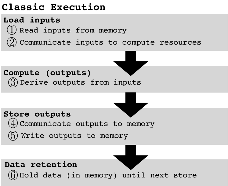
Both the breakdown of total power consumption across events, and the ratio of dynamic to static power per event evolve as a function of the operating regime and technology. Unfortunately, emerging technology solutions are not mature enough to meet the growing performance, storage capacity, and communication bandwidth demand within the tightly bound power budget (mainly due to cooling and power delivery limitations). At the same time, imbalances between logic and memory technologies cause energy (time $\times$ power) consumption of data loads and stores (①, ②, ④ and ⑤) to significantly exceed the energy consumption of actual computation (③) [3, 11]. As a consequence, reproducing, i.e., recomputing data can become more energy efficient than storing and retrieving pre-computed data. This discrepancy is expected to become even more prevalent with technology scaling [15].

Figure 2: Classic execution vs. Recomputation

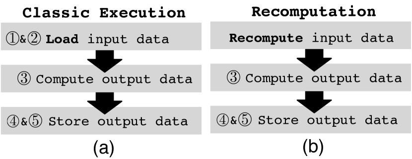
Figure 2(a) shows the classic trajectory at each step of execution. Black arrows point to the direction of data flow. As depicted in Figure 2(b), recomputation swaps load instructions for the reproduction of the respective input operands (which would otherwise be loaded from memory) for the subsequent computation. ① incurs the time and power overhead of the memory (hierarchy) access to perform the load; ②, of the subsequent communication of inputs to compute resources. Recomputation transforms the overhead of ① & ② to the overhead of the recomputation of the respective data values, i.e., of ③. Therefore, recomputation can only improve energy efficiency if the cost of data reproduction remains less than the overhead of ① & ②. In other words, the overhead of ① & ② sets the budget for recomputation.

Recomputation can also reduce the pressure on memory capacity and communication bandwidth. A recomputing processor can accommodate more compute resources (in the form of general-purpose cores or specialized accelerators) to occupy the area once allocated to memory (hierarchy). At the same time, under recomputation the workload becomes more compute-intensive to make a better use of classic processors optimized for compute performance, as opposed to energy efficiency. This paper quantitatively characterizes the energy efficiency potential of recomputation, and introduces a taxonomy for the computation vs. communication trade-off. In the following, Section 2 introduces the taxonomy; Sections 3 and 4 provide the evaluation; Section 5 covers related work, and Section 6 summarizes the findings.

2 Recomputation Taxonomy

The energy overhead of the load from Figure 2(a) determines the energy budget for recomputation. Unless the energy cost of reproducing data remains less than the energy cost of the respective load, recomputation cannot improve energy efficiency. Whether recomputation can improve energy efficiency or not tightly depends on where the data reside in the memory hierarchy – it is the location of the data in the memory hierarchy which determines the energy cost of the load. On the other hand, recomputation also incurs an energy cost due to the introduction of recomputing, producer instructions.

The taxonomy of recomputation techniques spans three dimensions. Recomputation can reproduce the data (which otherwise would be loaded from memory) by brute-force recalculation [1], value prediction [12, 22], or approximation [21, 24], respectively:

• Under brute-force recalculation, the recomputation effort goes to the derivation of data values, by re-executing the producer instructions (of the data values, which would otherwise be loaded from memory).

• Under prediction, the recomputation effort goes to the estimation of data values by exploiting value locality – the likelihood of the recurrence of data values [22] within the course of execution.

• Under approximation, the recomputation effort goes to the actual calculation of data values – as it is the case for brute-force recalculation, however, at reduced accuracy. In this case, the compute resources may only partially execute the producer instructions (e.g., by dropping a subset), or perform recomputation on reduced-accuracy hardware.

Depending on the accuracy of prediction or approximation of the data values, prediction or approximation may degrade accuracy of the end results, which is not the case for brute-force recalculation. This paper focuses on recalculation and prediction, and leaves approximation based recomputation to future work.

2.1 Recalculation Based Recomputation

Recalculation can be implemented in various ways. We use compiler-based proof-of-concept implementation similar to  [1]. During code generation, the compiler replaces each energy-hungry load instruction with the sequence of (arithmetic/logic) producer instructions of the respective data values. To this end, the compiler recursively traces data dependencies. The sequence of producer instructions forms a backwards slice, referred as Recalculation Slice, RSlice [1].

Figure 3: Example Recalculation Slice (RSlice)

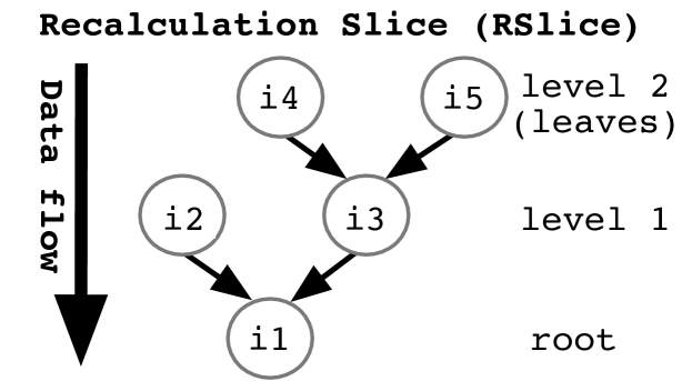
Fig. 3 demonstrates an example RSlice. Each RSlice is an upside-down tree, with nodes representing producer instructions to be re-executed. Data flows from the leaves to the root. The node at the root corresponds to the immediate producer of the data value which would otherwise be loaded from memory. Nodes at level 1 correspond to the producers of the root. Nodes at level l correspond to the producers of nodes at level l-1. The number of incoming arrows at each node reflects the number of producers (of the node) to be re-executed. The leaf nodes either represent terminal instructions which do not have any producers, or instructions for which re-execution of their producers is not energy efficient. In the proof-of-concept implementation, the compiler is in charge of making sure that all input operands of producer instructions within an RSlice are available at the anticipated time of recalculation. Unless the compiler guarantees this constraint, an RSlice cannot replace its respective load in the binary.

The compiler swaps a load with its respective RSlice only if recalculation of the corresponding data value along the RSlice is more energy efficient than performing the load.

2.2 Prediction Based Recomputation

Under prediction, the recomputation effort goes to the estimation of data values, instead of brute-force recalculation. Accurate estimation is only possible if data values (which otherwise would be loaded from memory) exhibit high value locality – i.e., a high likelihood of recurrence [22] within the course of execution. For example, if a data value exhibits excellent (100%) locality, just storing the value in a dedicated buffer and retrieving it from there may turn out to be more energy efficient than recalculating it (Section 2.1) or loading it from memory. Even if the value locality remains less than 100%, such buffered history of values can be used for prediction. It has been shown that emerging applications can oftentimes mask prediction incurred inaccuracy due to potential errors in estimation, as implied by imperfect value locality [22].

Value retrieval from the history buffer constitutes the main cost of prediction. Under imperfect value locality, a prediction algorithm can help estimate the respective value by using the buffered history of previously observed values. In this case, the cost of executing the prediction algorithm should also be considered. The overall cost of prediction should fit into the recomputation budget, which in turn is set by the energy overhead of the respective load. Prediction based recomputation can only be beneficial if its energy cost remains less than the energy overhead of this load.

2.3 Recalculation + Prediction

Prediction based recomputation (Section 2.2) exploits locality of data values which would otherwise be loaded from memory. With respect to recalculation (Section 2.1), prediction targets the value to be produced by the root node of the RSlice. Input values of RSlice nodes may also exhibit significant value locality. Let us assume that such a node n resides at level l, and it is not a leaf. In this case, predicting n’s inputs may turn out to be more energy efficient than re-executing n’s producers residing at level l+1 of the RSlice. Hence, combining recalculation with prediction (i.e., recalculation + prediction) can result in pruned RSlices to harvest even more energy efficiency. Prediction can also serve identifying the inputs of leaves – recall that, if retrieving input data of leaves requires energy hungry memory accesses, recalculation along the RSlice cannot be of any use. Each intermediate node of the RSlice subject to prediction becomes practically a leaf, as re-execution past such nodes would no longer be necessary.

Recalculation + prediction can prune RSlices, however, even under pure recalculation (Section 2.1), RSlices can never grow excessively: the energy overhead of the respective load determines the budget for recomputation. The cost of recalculation increases with the number of levels, i.e., height of the RSlice, and the number of nodes residing at each level. The re-execution of each node instruction incurs an energy cost. At most, as many nodes can be re-executed (i.e., can reside in the RSlice) as can be fit into the recomputation budget. And recalculation can only improve energy efficiency if the cost of re-execution along the RSlice remains less than the recomputation budget, which is set by the energy overhead of the respective load. In this manner, the energy overhead of the load prevents excessive growth of the RSlice. Under recalculation + prediction, the cost of re-execution along the RSlice along with the cost of selective prediction constitute the cumulative cost of recomputation.

3 Evaluation Setup

We experiment with benchmarks from the SPEC2006 [10], PARSEC [4], NAS [2], and Rodinia [7] suites, which span emerging application domains (Table 1). In the evaluation, we only analyze the benchmarks which harvest sizable energy efficiency gain under recomputation. The rest of the benchmarks did not benefit from recomputation. The analyzed mix contains both compute- and memory-intensive applications. Our analysis is confined to sequential, i.e., single-threaded execution. We leave parallel recomputation to future work. We use a cycle accurate micro-architectural simulator, Sniper [6]. The simulated microarchitecture is modeled after an in-order single-core Intel Xeon Phi-like processor without loss of generality, which features an operating frequency of 1.09GHz at 22nm, an L1 instruction cache of 32KB (4-way, LRU), an L1 data cache of 32KB (8-way, LRU, WB), and an L2 cache of 512KB (8-way, LRU, WB). We profile the native binaries (conforming to classic execution, hence excluding recomputation) of the benchmarks on Sniper: We record (i) value locality of instructions at runtime (to be exploited by prediction based recomputation); (ii) cache statistics, i.e., hit and miss rates, at runtime (to derive the probabilistic energy cost model of the compiler pass as explained in Section 2.1).

Table 1: Benchmarks deployed

Suite	Benchmark	Input	Application Domain
SPEC	429.mcf (mcf)	test	Combinatorial Optimization
SPEC	482.sphinx3 (sx)	test	Speech Recognition
NAS	is	A	Integer Sorting
PARSEC	canneal (ca)	simsmall	Routing Cost Minimization
PARSEC	facesim (fs)	simsmall	Motion Simulation
PARSEC	ferret (fe)	simsmall	Content Similarity Search
PARSEC	raytrace (rt)	simsmall	Real-time Raytracing
Rodinia	backpropagation (bp)	65536	Pattern Recognition
Rodinia	breath-first search (bfs)	graph1MW_6.txt	Graph Traversal
Rodinia	srad (sr)	100 0.5 502 458 1	Image Processing

Probabilistic Energy Cost Model for the Compiler Pass from Section 2.1: The energy per instruction (EPI) estimates per load, store, and non-memory instructions come from measured Xeon Phi data from [26], which for memory instructions, provides separate EPI estimates for each level Li in the memory hierarchy: EPI_Li. Using these EPI_Li and cache statistics from Sniper, we extract probabilistic EPI estimates for loads as follows: We derive Pr_Li, the probability of having the load serviced by level Li, using hit and miss statistics of Li from Sniper. Then, the sum of Pr${}_{Li}\times$ EPI_Li over all levels $i$ in the memory hierarchy gives the probabilistic energy cost per load. Using this energy cost per load, and the EPIs for non-memory instructions, the compiler pass swaps a load with its respective RSlice only if recalculation of the corresponding data value along the RSlice incurs a lower energy cost than performing the load.

Simulation Infrastructure: We implement the compiler pass from Section 2.1 in a Pin [23] based tool, which by using the probabilistic energy cost model detailed above and by tracking data dependencies, swaps load instructions in the binary for the respective RSlices, only if recomputation incurs a lower energy consumption. This tool adjusts the binary under prediction and recalculation+prediction accordingly, following Sections 2.2 and 2.3. We restrict prediction with the prediction of the values to be produced by RSlice roots. We deploy Sniper integrated with McPAT [20] to run these annotated binaries in order to collect performance and energy statistics under recomputation.

4 Evaluation

We next quantify the energy efficiency under recomputation and analyze the implications for execution semantics.

4.1 Impact on Energy and Performance

Figure 4: Energy gain under recomputation.

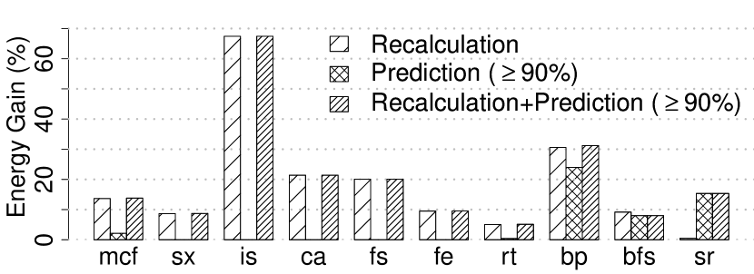
Figure 4 compares the energy consumption under recalculation, prediction, and recalculation+prediction based recomputation. This analysis accounts for the overhead of recomputing producer instructions (along RSlices) under recalculation (Section 2.1), and history buffer accesses under prediction (Section 2.2). However, we assume that one history buffer access suffices for value prediction at 100% accuracy (i.e., we omit any potential overhead due to prediction algorithms). For this experiment, we set the value locality threshold to enable prediction to 90%: prediction only applies to instructions which exhibit at least 90% value locality. Prediction targets only the values to be re-produced by root instructions of RSlices (all instructions along which are re-executed under recalculation). Under recalculation+prediction, on the other hand, prediction can target any RSlice instruction but the root (Section 2.3).

Figure 4 reports the energy gain with respect to native execution, which excludes recomputation. We observe that except bp, bfs and sr, the energy gain under prediction is insignificant. This is because only a small of number of instructions exhibit a higher value locality than 90%. Due to its wider applicability, recalculation unlocks higher energy gains, ranging from 5.06% to 67.43%, except sr. The recalculation cost for sr remains generally higher than the cost of the respective loads. An interesting observation is that bfs obtains lower energy gain under prediction and recalculation+prediction when compared to recalculation alone. The reason is that the RSlices of bfs are very short, rendering recalculation always cheaper than prediction. At the same time, our proof-of-concept implementation gives the priority to prediction, if a value exceeds the locality threshold set for prediction (i.e., 90%) under recalculation+prediction: in other words, we omit recalculation for all values that exhibit a higher value locality than the threshold (90% in this case), even though recalculation turns out to be less energy hungry than the respective load. Therefore, the energy gain under recalculation+prediction cannot exceed the gain under recalculation for bfs. Overall, the energy gain due to recalculation+prediction remains limited for the majority of the benchmarks. The reason is twofold: the benchmarks either do not have enough value locality to exploit prediction (e.g. mcf, sx, is, ca, fs, fe, and rt), or recalculation is too costly (e.g. sr).

Figure 5: Performance improvement under recomputation.

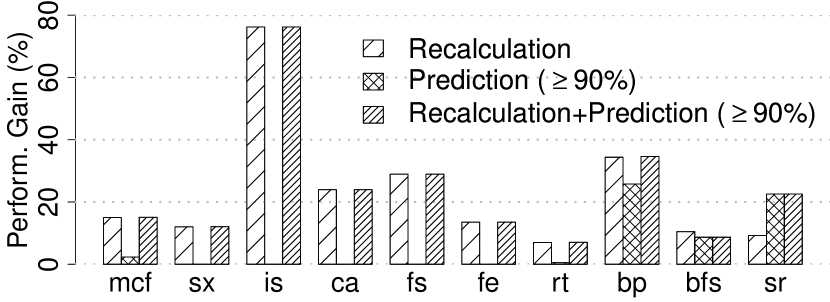
Figure 5 reports the corresponding improvement in performance (i.e., execution time) with respect to native execution. Generally, a similar trend to energy gain applies, except that the performance gain under recalculation for sr becomes more pronounced when compared to the energy gain.

Figure 6: EDP gain under recomputation.

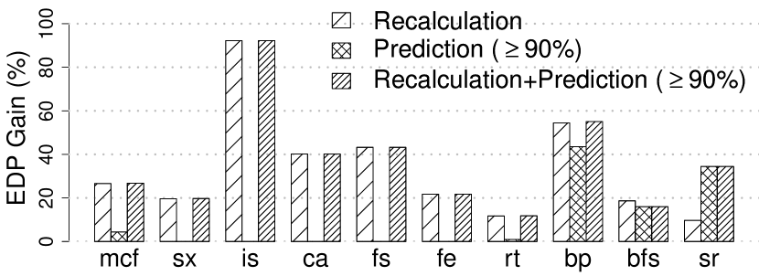
Figure 6 summarizes the resulting gain in energy efficiency in terms of EDP (energy delay product [8]), with respect to native execution. Overall, recalculation+prediction maximizes the EDP gain, and recalculation remains effective as well, except sr (as explained above). Prediction is beneficial for bp, bfs, and sr only – recall that even this gain under prediction is optimistic as we neglect any algorithmic overhead. Finally, recalculation+prediction results in 11.8% to 92.2% EDP gain across all benchmarks.

Figure 7: EDP gain under prediction as a function of value locality threshold for prediction.

Figure 8: EDP gain under recalculation+prediction as a function of value locality threshold for prediction.

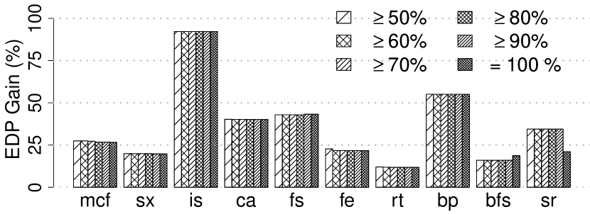
We next assess the sensitivity of EDP gain to the value locality threshold for prediction. Figure 7 reports the EDP gain under prediction; Figure 8, under recalculation+prediction, as we sweep the threshold between 50% and 100%. Each bar per benchmark represents a different value locality threshold from this range to enable prediction. Generally, as the threshold increases, the number of instructions exhibiting at least that much locality reduces – therefore, a lower number of predictions can be performed, and both the energy and performance gains drop accordingly. Among the benchmarks, bp exhibits the highest value locality, hence, it benefits most from prediction. bfs and sr, as well, benefit from prediction if the threshold remains lower than 100% – as very small number of loads swapped for RSlices feature 100% value locality for these benchmarks. On the other hand, fs and mcf harvest sizable EDP gain under prediction only if the threshold remains lower than 90% and 80%, respectively. The remaining benchmarks have a very small number of load instructions that exhibit $\geq$ 50% value locality, so only a negligible EDP gain applies under prediction (which already represents an upper limit for actual gains, as we neglect any algorithmic overhead). Therefore, recalculation+prediction can generally provide higher EDP gains when compared to prediction. As mentioned before, bfs has small RSlices, thus, the associated recalculation cost usually remains lower than than the cost of prediction. Accordingly, bfs shows higher EDP gain for 100% threshold (at which a smaller number of values can be predicted, by definition, when compared to lower values of the threshold) under recalculation+prediction. Overall, we observe that our findings from Figure 6 generally apply over this wider range of threshold values. We can conclude that recalculation has wider coverage for recomputation than prediction. Next, we investigate why this is the case.

(a) mcf

(b) sphinx3

(c) is

(d) canneal

(e) facesim

(f) ferret

(g) raytrace

(h) backpropagation

(i) bfs

(j) srad

Figure 9: Value locality of RSlice instructions.

4.2 Impact on Execution Semantics

(a) mcf

(b) sphinx3

(c) is

(d) canneal

(e) facesim

(f) ferret

(g) raytrace

(h) backpropagation

(i) bfs

(j) srad

Figure 10: Node count of RSlices before (recalculation) and after pruning (recalculation+prediction).

As explained in Sections 2.2 and 2.3, in the context of recomputation, prediction serves two purposes:
(i) to predict the values which would otherwise be loaded from memory (and which correspond to the values to be re-produced by RSlice roots under pure recalculation) under prediction;
(ii) to predict the input values of intermediate (non-root) RSlice nodes under recalculation+prediction.

Prediction can eliminate re-execution along an entire RSlice if the values to be re-produced by the RSlice root (i.e., the values which would otherwise be loaded from memory) exhibit sufficiently high locality. recalculation+prediction, on the other hand, can prune any intermediate RSlice node (except the root) exhibiting sufficient (input) value locality to render a smaller RSlice, which in turn becomes less energy costly to execute.

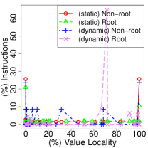
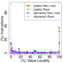
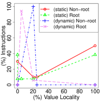
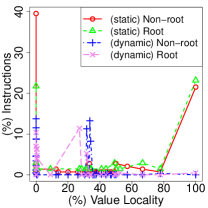
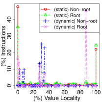
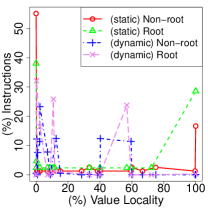
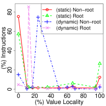
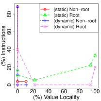
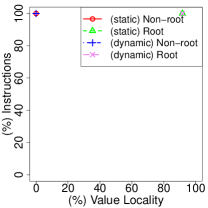
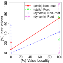
For prediction based recomputation to work, the respective instructions should exhibit sufficiently high value locality. Figure 9 reports a histogram of % value locality (x-axis) for all instructions residing in RSlices. The y-axis reports the % share of instructions exhibiting a given value of locality on the x-axis. Root captures the output value locality of RSlice roots; Non-root, the input value locality of intermediate (non-root) RSlice nodes. Recall that the output value locality of RSlice roots corresponds to the value locality of the respective load instructions which are replaced by RSlices.

Notice the distinction between static and dynamic instructions (for both root and non-root, i.e., intermediate instructions). Static instructions are the ones that are embedded in the binary by the compiler. Dynamic instructions are the ones that are actually executed at runtime. A static instruction may have multiple dynamic instances executed at runtime, or may not be executed at all. This distinction helps us to explain why, for instance, we do not obtain much benefit from prediction although a great fraction of static instructions have high value locality for is (Figure 9c): 38.46% of (static) root instructions of is have 100% value locality, but is does not benefit much from prediction (Figure 7). This is because, at runtime, the root instructions having 100% value locality are not executed as many times as other root instructions that have lower value locality. In fact, less than 1% of dynamic root instructions executed have 100% value locality for is, as shown in Figure 9c. The previous section revealed that bp benefits from prediction the most (Figure 7). Therefore, we expect a larger fraction of roots to have very high value locality for this benchmark. Figure 9h reveals that 20% of dynamic root instructions of bp have 100% value locality indeed. A similar trend holds for non-root instructions under recalculation+prediction. For recalculation+prediction, prediction of non-root instructions can provide sizable gains only if the dynamic share of non-root instructions exhibiting high value locality is large.

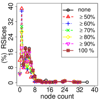
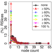
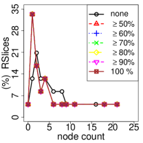
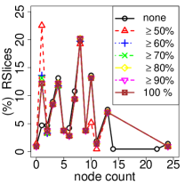
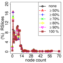
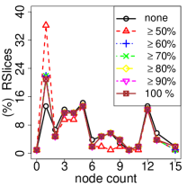
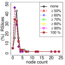
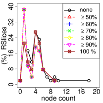
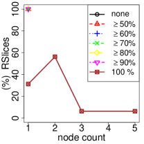
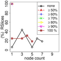
Figure 10 shows how the node count of RSlices change as the locality threshold to enable prediction increases from 50% to 100% under recalculation+prediction – none reflects no prediction, i.e., pure recalculation. The figure reports a histogram of node count of RSlice (x-axis). The y-axis reports the % share of RSlices having a given node count on the x-axis. A lower threshold enables more predictions, hence more producer instructions can get pruned, and the node count shrinks more. We observe that prediction at a value locality threshold of 50% can reduce the node count of RSlices up to 56%.

5 Related Work

Amnesiac [1] trades off computation for communication by replacing energy hungary loads with a set of low-energy arithmetic/logic instructions that are responsible for generating data to be loaded. This reduces the amount of energy consumed on data communication. We use similar compiler-based proof-of-concept recalculation implementation. Kandemir et al. proposed recomputation to reduce off-chip memory area in embedded processors [13]. Koc et al. investigated how recomputation of data residing in memory banks in low-power states can reduce the energy consumption by preventing frequent switching of the corresponding banks to high-power states for data retrieval [17]. Koc et al. further devised recomputation-aware compiler optimizations for scratchpad memories [16]. The compiler strategies from [17] and [16] are confined to array variables. In our paper, recomputation is not limited to embedded processors or specific data structures. DataScalar [5] trades off computation for communication by replicating data in each processor’s local memory in a distributed environment. Accordingly, Datascalar divides the program address space between replicated and communicated pages. Our framework trades off computation for storage, hence minimizes communication rather as a side effect. As opposed to DataScalar, our framework can reduce the program memory footprint. Our study analyzes recomputation at a finer granularity. Processing in/near memory [28, 18, 25, 14, 19] can bridge the gap between logic and memory speeds by embedding compute capability in/near memory. Processing in memory can minimize energy-hungry data transfers, as well, and is orthogonal to recomputation. Memoization [27, 9] – the dual of recomputation – replaces (mainly frequent and expensive) computation with table look-ups for pre-computed data. Similar to processing in memory and recomputation, memoization can mitigate the communication overhead (as long as table look-ups remain cheaper than long-distance data retrieval). Memoization and recomputation can complement each other in boosting energy efficiency.

6 Conclusion

Recomputation can minimize, if not eliminate, the prevalent power and performance (hence, energy) overhead incurred by data storage, retrieval, and communication, thus, render more energy efficient execution. This paper provided a quantitative proof-of-concept analysis for the computation vs. communication trade-off, along with a taxonomy. Recomputation replaces data load(s) from memory with the reproduction of the respective data. Unless the energy cost of reproducing data remains less than the energy cost of retrieving it from memory, recomputation cannot improve energy efficiency.

In this study, we explored (interactions between) two broad classes of recomputation techniques: brute-force recalculation and prediction based recomputation. Under recalculation, the recomputation effort goes to the derivation of the data values (which would otherwise be loaded from memory), by re-executing the producer instruction(s) of the eliminated load(s). Under prediction, the recomputation effort goes to the estimation of the data values by exploiting value locality – the likelihood of the recurrence of values (which would otherwise be loaded from memory) within the course of execution. We find that recalculation has wider coverage for recomputation than prediction, as prediction cannot be effective under limited value locality.

References

- [1] Ismail Akturk and Ulya R Karpuzcu. AMNESIAC: Amnesic Automatic Computer - Trading Computation for Communication for Energy Efficiency. In International Conference on Architectural Support for Programming Languages and Operating Systems, 2017.
- [2] D. H. Bailey, E. Barszcz, J. T. Barton, D. S. Browning, R. L. Carter, L. Dagum, R. A. Fatoohi, P. O. Frederickson, T. A. Lasinski, R. S. Schreiber, H. D. Simon, V. Venkatakrishnan, and S. K. Weeratunga. The NAS parallel benchmarks–summary and preliminary results. In Conference on High Performance Computing Networking, Storage and Analysis, pages 158–165, 1991.
- [3] K Bergman, S Borkar, D Campbell, W Carlson, W Dally, M Denneau, P Franzon, W Harrod, J Hiller, and S Karp. Exascale computing study: Technology challenges in achieving exascale systems. DARPA Information Processing Techniques Office (IPTO) sponsored study, 2008.
- [4] Christian Bienia, Sanjeev Kumar, Jaswinder Pal Singh, and Kai Li. The PARSEC Benchmark Suite: Characterization and Architectural Implications. Technical Report TR-811-08, Princeton University, January 2008.
- [5] D Burger, S Kaxiras, and J R Goodman. Datascalar Architectures. In International Symposium on Computer Architecture, June 1997.
- [6] Trevor E. Carlson, Wim Heirman, and Lieven Eeckhout. Sniper: Exploring the level of abstraction for scalable and accurate parallel multi-core simulation. In SC, November 2011.
- [7] Shuai Che, Michael Boyer, Jiayuan Meng, David Tarjan, Jeremy W. Sheaffer, Sang-Ha Lee, and Kevin Skadron. Rodinia: A Benchmark Suite for Heterogeneous Computing. In IISWC, 2009.
- [8] R Gonzalez and M Horowitz. Energy dissipation in general purpose microprocessors. JSSC, 31(9):1277–1284, 1996.
- [9] Xiaochen Guo, Engin Ipek, and Tolga Soyata. Resistive computation: avoiding the power wall with low-leakage, STT-MRAM based computing. In International Symposium on Computer Architecture, 2010.
- [10] John L. Henning. SPEC CPU2006 benchmark descriptions. SIGARCH Computer Architecture News, 34(4), September 2006.
- [11] Mark Horowitz. Computing’s Energy Problem (and what we can do about it). Keynote at ISSCC, 2014.
- [12] Jian Huang and D.J. Lilja. Exploiting Basic Block Value Locality With Block Reuse. In International Symposium on High Performance Computer Architecture, 1999.
- [13] M Kandemir, Feihul Li, Guilin Chen, Guangyu Chen, and O Ozturk. Studying storage-recomputation tradeoffs in memory-constrained embedded processing. In Design, Automation and Test in Europe, 2005.
- [14] Yi Kang, Wei Huang, Seung-Moon Yoo, D. Keen, Zhenzhou Ge, V. Lam, P. Pattnaik, and J. Torrellas. Flexram: toward an advanced intelligent memory system. In International Conference on Computer Design, 1999.
- [15] S W Keckler, W J Dally, B Khailany, M Garland, and D Glasco. GPUs and the Future of Parallel Computing. IEEE Micro, 31(5), 2011.
- [16] H Koc, M Kandemir, E Ercanli, and O Ozturk. Reducing Off-Chip Memory Access Costs Using Data Recomputation in Embedded Chip Multi-processors. In Design Automation Conference, 2007.
- [17] H Koc, O Ozturk, M Kandemir, and E Ercanli. Minimizing Energy Consumption of Banked Memories Using Data Recomputation. In International Symposium on Low-Power Electronics and Design, 2006.
- [18] P. M. Kogge. The EXECUBE approach to massively parallel processing. In International Conference on Parallel Processing, 1994.
- [19] P.M. Kogge, S.C. Bass, J.B. Brockman, D.Z. Chen, and E. Sha. Pursuing a petaflop: point designs for 100 TF computers using PIM technologies. In Frontiers of Massively Parallel Computing, 1996.
- [20] Sheng Li, Jung Ho Ahn, Richard D. Strong, Jay B. Brockman, Dean M. Tullsen, and Norman P. Jouppi. McPAT: An Integrated Power, Area, and Timing Modeling Framework for Multicore and Manycore Architectures. In International Symposium on Microarchitecture, 2009.
- [21] K. J. Lin, S. Natarajan, and J. W. S. Liu. Imprecise Results: Utilizing Partial Computations in Real-Time Systems. In Real-Time Systems Symposium, 1987.
- [22] Mikko H Lipasti, Christopher B Wilkerson, and John Paul Shen. Value Locality and Load Value Prediction. In International Conference on Architectural Support for Programming Languages and Operating Systems, 1996.
- [23] Chi-Keung Luk, Robert Cohn, Robert Muth, Harish Patil, Artur Klauser, Geoff Lowney, Steven Wallace, Vijay Janapa Reddi, and Kim Hazelwood. Pin: Building Customized Program Analysis Tools with Dynamic Instrumentation. In Programming Language Design and Implementation, 2005.
- [24] Joshua San Miguel, Mario Badr, and Natalie Enright Jerger. Load Value Approximation. In International Symposium on Microarchitecture, 2014.
- [25] David Patterson et al. A case for intelligent RAM. IEEE Micro, 17(2):34–44, 1997.
- [26] Y.S. Shao and D. Brooks. Energy characterization and instruction-level energy model of Intel’s Xeon Phi processor. In International Symposium on Low-Power Electronics and Design, September 2013.
- [27] A Sodani and G S Sohi. Dynamic Instruction Reuse. In International Symposium on Computer Architecture, 1997.
- [28] Harold S. Stone. A logic-in-memory computer. IEEE Transactions on Computers, C-19(1), Jan 1970.