Semiclassical analysis of elastic surface waves
Abstract
In this paper, we present a semiclassical description of surface waves or modes in an elastic medium near a boundary, in spatial dimension three. The medium is assumed to be essentially stratified near the boundary at some scale comparable to the wave length. Such a medium can also be thought of as a surficial layer (which can be thick) overlying a half space. The analysis is based on the work of Colin de Verdière [11] on acoustic surface waves. The description is geometric in the boundary and locally spectral “beneath” it. Effective Hamiltonians of surface waves correspond with eigenvalues of ordinary differential operators, which, to leading order, define their phase velocities. Using these Hamiltonians, we obtain pseudodifferential surface wave equations. We then construct a parametrix. Finally, we discuss Weyl’s formulas for counting surface modes, and the decoupling into two classes of surface waves, that is, Rayleigh and Love waves, under appropriate symmetry conditions.
1 Introduction
We carry out a semiclassical analysis of surface waves in a medium which is stratified near its boundary – with topography – at some scale comparable to the wave length. We discuss how the (dispersive) propagation of such waves is governed by effective Hamiltonians on the boundary and show that the system is displayed by a space-adiabatic behavior.
The Hamiltonians are non-homogeneous principal symbols of some pseudodifferential operators. Each Hamiltonian is identified with an eigenvalue in the point spectrum of a locally Schrödinger-like operator in dimension one on the one hand, and generates a flow identified with surface-wave bicharacteristics in the two-dimensional boundary on the other hand. The eigenvalues exist under certain assumptions reflecting that wave speeds near the boundary are smaller than in the deep interior. This assumption is naturally satisfied by the structure of Earth’s crust and mantle (see, for example, Shearer [36]). The dispersive nature of surface waves is manifested by the non-homogeneity of the Hamiltonians.
The spectra of the mentioned Schrödinger-like operators consist of point and essential spectra. The surface waves are identified with the point spectra while the essential spectra correspond with propagating body waves. We note, here, that the point and essential spectra for the Schrödinger-like operators may overlap.
Our analysis applies to the study of surface waves in Earth’s “near” surface in the scaling regime mentioned above. The existence of such waves, that is, propagating wave solutions which decay exponentially away from the boundary of a homogeneous (elastic) half-space was first noted by Rayleigh [34]. Rayleigh and (“transverse”) Love waves can be identified with Earth’s free oscillation triples and with assuming spherical symmetry. Love [23] was the first to argue that surface-wave dispersion is responsible for the oscillatory character of the main shock of an earthquake tremor, following the “primary” and “secondary” arrivals.
Our analysis is motivated by the (asymptotic) JWKB theory of surface waves developed in seismology by Woodhouse [44], Babich, Chichachev and Yanoskaya [3] and others. Tromp and Dahlen [40] cast this theory in the framework of a “slow” variational principle. The theory is also used in ocean acoustics [6] and is referred to as adiabatic mode theory. An early study of the propagation of waves in smoothly varying waveguides can be found in Bretherton [5]. Nomofilov [30] obtained the form of WKB solutions for Rayleigh waves in inhomogeneous, anisotropic elastic media using assumptions appearing in Proposition 6 in the main text. Many aspects of the propagation of surface waves in laterally inhomogeneous elastic media are discussed in the book of Malischewsky [24]. Here, we develop a comprehensive semiclassical analysis of elastic surface waves, generated by interior (point) sources, with the corresponding estimates. This semiclassical framework was first formulated by Colin de Verdière [11] to describe surface waves in acoustics.
The scattering of surface waves by structures, away from the mentioned scaling regime, has been extensively studied in the seismology literature. This scattering can be described using a basis of local surface wave modes that depend only on the “local” structure of the medium, for example, with invariant embedding; see, for example, Odom [31]. Odom used a layer of variable thickness over a homogeneous half space to account for the interaction between surface waves and body waves by the topography of internal interfaces.
The outline of this paper is as follows. In Section 2, we carry out the semiclassical construction of general surface wave parametrices. In the process, we introduce locally Schrödinger-like operators in the boundary normal coordinate and their eigenvalues signifying effective Hamiltonians in the boundary (tangential) coordinates describing surface-wave propagation. In Section 3, we characterize the spectra of the relevant Schrödinger-like operators. That is, we study their discrete and essential spectra. In Section 4, we consider a special class of surface modes associated with exponentially decaying eigenfunctions. The existence of such modes is determined by a generalized Barnett-Lothe condition. In Section 5, we review conditions on the symmetry, already considered by Anderson [1], restricting the anisotropy to transverse isotropy with the axis of symmetry aligned with the normal to the boundary, allowing the decoupling of surface waves into Rayleigh and Love waves. In Section 6, we establish Weyl’s laws first in the isotropic (separately for Rayleigh and Love waves) and then in the anisotropic case. Finally, in Section 7, we relate the surface waves to normal modes viewing the analysis locally on conic regions, or more generally on Riemannian manifolds with a half cylinder structure. We give explicit formulas for the special case of a radial manifold.
2 Semiclassical construction of surface-wave parametrices
We consider the linear elastic wave equation in ,
| (1) |
where is the displacement vector, and is the stress tensor given by Hooke’s law
| (2) |
and denotes the strain tensor; is the fourth-order stiffness tensor with components , and is the density of mass. The componentwise expression of is given by
Equation (1) differs from the usual system given by
in case is not a constant. However, the difference is in the lower terms. These can be accounted for considering (1).
We study the elastic wave equation in the half space , with coordinates,
We consider solutions, , satisfying the Neumann boundary condition at ,
| (3) |
where
In the above, we assume that with
for some and satisfies the following symmetries and strong
convexity condition:
(symmetry) for any ;
(strong convexity) there exists such that for any nonzero
real-valued symmetric matrix ,
We note that these are physically very natural assumptions. We invoke, additionally,
Assumption 2.1.
The stiffness tensor and density obey the following scaling,
and, for any ,
where is the so-called limiting velocity which will be defined in Section 3.
2.1 Schrödinger-like operators
Under Assumption 2.1, we make the following change of variables,
upon introducing , the elastic wave equation in (3) takes the form
| (4) |
where
| (5) |
With Definition 11 in Appendix A, we consider as a semiclassical pseudodifferential operator on , where belongs to; then can be rewritten as
| (6) |
where is a semiclassical pseudodifferential operator with symbol defined by
with
| (7) |
and
| (8) |
We view and as ordinary differential operators in , with domain
2.2 Effective Hamiltonians
We use eigenvalues and eigenfunctions of to construct approximate solutions to . For fixed , an eigenvalue and the corresponding eigenfunction of are such that
| (9) |
where . Since is a positive symmetric operator in for , is real-valued, and also positive. We note, here, that the contribution coming from confined to a compact set is negligible. This is why we can assume that .
We let denote the set of all bounded operators from a normed space to a normed space .
Theorem 1.
Let be an eigenvalue of , and be open. Assume that has constant multiplicity for all . There exist and which admits asymptotic expansions
| (10) |
and satisfy
| (11) |
where denotes the composition of symbols (see Appendix A). Furthermore, and is the projection onto the eigenspace associated with .
Proof.
First, we note that (cf. Appendix B of [12]). By the composition of symbols (cf. Appendix A), we have
and
We construct the terms by collecting terms of equal orders in the two expansions above. Terms of order give
which is consistent with (9). Terms of order give
where denotes the remaining terms. We choose , so that, for , is orthogonal to the eigenspace of . Then we let be the unique solution of
which is orthogonal to the eigenspace of . Thus we have defined the operator . Higher order terms , , can be constructed successively by solving the equations,
with , since
, , in their respective
topologies, depend continuously on by induction. Hence, we
can choose
and solve for
. This completes the construction of
and .
∎
For any bounded set , we let be such that and with on . Then
| (12) |
defines a linear map on (the factor is to make the operator (microlocally) unitary), where
and denotes the space of microfunctions on ; see, Definition 14 of Appendix A. Moreover, we find that, using Theorem 1,
| (13) |
where the left- and right-hand sides are considered as microfunctions.
Remark 2.1.
We note that the principal symbol of is real-valued. Hence, the propagation of wavefront set of surface waves is purely on the the surface. However, since the lower order terms of are operators in , there exists coupling of surface waves with interior motion. There is no such coupling if the eigenvalue has multiplicity one. For this case is a classical pseudodifferential symbol.
2.3 Surface-wave equations and parametrices
With the results of the previous subsection, we construct approximate solutions of the system (3) with initial values
Then we construct solutions of the form
| (14) |
with
Here, is chosen such that for each , there are at least eigenvalues for . We assume that all eigenvalues are of constant multiplicities, . We let solve the initial value problems
| (15) | |||||
| (16) |
. Equation (16) means that the initial values are in the span of the ranges of operators , .
We address the existence of eigenvalues of in later sections, under the Assumption 2.1. To construct the parametrix, we use the first-order system for that is equivalent to (15),
| (17) |
We write . The principal symbol of is given by . Then
| (18) |
satisfy the two first-order (“half wave”) equations
| (19) |
where
| (20) |
supplemented with the initial conditions
| (21) |
The principal symbol of is given by defining a Hamiltonian. The solution to the original problem is then given by
| (22) |
We construct WKB solutions for operator , introducing a representation of the solution operator of the form,
| (23) |
Construction of the phase function. Surface-wave bicharacteristics are solutions, , to the Hamiltonian system,
| (24) |
We define
For in , the map
is surjective for small . We write and introduce the phase function
| (25) |
where denotes the inner product of and . This phase function solves
[45, Chapter 10]. The group velocity, , is defined by
| (26) |
We note that is non-homogeneous in , thus the group velocity and the bicharacteristics depend on .
Construction of the amplitude. The amplitude in (23) must satisfy
or, equivalently,
| (27) |
We note that appears in the construction of the phase function . We construct solutions, , via the expansion,
and writing the symbol of as an expansion,
By the asymptotics of , the terms of order yield the equation,
| (28) |
for the phase function , which was introduced above. The terms of order yield the transport equation for ,
where
| (29) |
in which , . Denote
For solving the transport equations, we use the bicharacteristics determined by (24). We note that
so that
The equations above can be solved using the standard theory of ordinary differential equations. For more details about semiclassical Fourier Integral Operators, we refer to Chapter 10 of Zworski’s book [45].
Trace. We can write the solution to (19), up to leading order, as
with
Then, using (18), (21) and (22), we can write down the approximate Green’s function (microlocalized in ), still up to leading order, for surface waves
| (30) |
Then
Now, we take the semiclassical Fourier transform in multiply by the test function and apply the stationary phase formula to the leading order (see, for example, [18], Proposition 5.2). We get
As , we get
On the diagonal , we get
We remember here that for (cf. (12)). Assuming the eigenvalues are all simple, we can simply take as normalized eigenfunctions. Then,
The left-hand side can be viewed as a local trace in the boundary normal coordinate.
Remark 2.2.
In the oscillatory integral , the phase variables are the components of . We can construct an alternative representation by using the frequency, , as a phase variable. This would result in the following form of solution operator
| (31) |
In a neighborhood of a fixed point, , we construct satisfying the eikonal equation
| (32) |
Then the phase function is given by
and satisfies ,
We consider the bicharacteristics
and let , while
. The generating function satisfies
and can then be written in the form
We mention an alternative representation. For any , we let , be the solution of
This is unique due to the monotonicity of eigenvalue in with respect to the quadratic form associated with . We denote with , and define the phase velocity, , as
| (33) |
Thus . Using and we find that
| (34) |
defined in a neighborhood of . Since is frequency dependent, the geodesic distance is frequency dependent.
3 Characterization of the spectrum of
In this section, we characterize the spectrum of . In the case of constant coefficients, that is, a homogeneous medium, the spectrum was described in [22]. In the case of isotropic media, the spectrum was studied by Colin de Verdière [9].
We view
as a semiclassical pseudodifferential operator with as the semiclassical parameter, say. We write and use to denote the Fourier variable for . Then the principal symbol of is given by
| (35) |
where
| (36) |
We follow [38] to define so-called limiting velocities. Let and be orthogonal unit vectors in which are obtained by rotating the orthogonal unit vectors and around their vector product by an angle :
For any , we write
We let
and note that
Definition 2.
The limiting velocity is the lowest velocity for which the matrices and become singular for some angle :
Remark 3.1.
In the isotropic case, that is,
where are the two Lamé moduli, we have
with and . The limiting velocity is given by
The spectrum of is composed of a discrete spectrum contained in and an essential spectrum, (Figure 1):
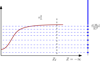
Theorem 3.
Under Assumption 2.1, the spectrum of is discrete below . The discrete spectrum is nonempty if is sufficiently large.
Proof.
We need some notation and a few facts from operator theory for the proof of this theorem. A brief review of those prerequisites are provided in Appendix B. For more details, we refer to [35]. We adopt the classical Dirchlet-Neumann bracketing proof. Here we use ′ to represent the partial derivative with respect to . Consider , and the corresponding quadratic form,
| (37) |
on , which is positive. We decompose into intervals , the interiors, , of which are disjoint. We let be a minimal element in the set,
(The order is defined as if for any symmetric matrix . This is then a partially ordered set, and a minimal element exists by Zorn’s lemma.) Similarly, we define to be a maximal element of
Furthermore, we introduce on .
We consider
for , and let be the unique self-adjoint operator on associated to the quadratic form (cf. Appendix B). This is equivalent to defining
| (38) |
on . Then
It follows that for each , has only a discrete spectrum, since it is a self-adjoint second-order elliptic differential operator on a bounded interval.
The spectrum of is also discrete below [38, Theorems 3.12, 3.13]. We note here that this property is related to the existence of surface waves for a homogenous half space. Thus the spectrum of below must be discrete (see the Lemma on pp. 270, Vol. IV of [35].)
We define as the unique self-adjoint operator on , the quadratic form of which is the closure of the form
with domain . This is equivalent to defining
| (39) |
on . Then
, for each , has a discrete and real spectrum. The operator also has a discrete spectrum below , since .
We suppose now that the decomposition is fine enough, and that for some has a limiting velocity . (There exists such that . Suppose for some . For any , if is small enough, . This show nonemptyness of . We can take small enough, so that has limiting velocity .) We let be the first eigenvalue of , and claim that . We prove this claim next.
We let . We note that
has a bounded solution, with , . To construct a solution of this form, we carry out a substitution and obtain
| (40) |
Here, are defined as in (36) for . The above system has a non-trivial solution if and only if
| (41) |
Since , there exists a real-valued solution to (41) ([38], Lemma 3.2). .
We let on and ; can be constructed such that , , . Then for some independent of . After renormalization, we can assume that . Then
| (42) |
When is small, that is, is large, has eigenvalues below . Then the discrete spectrum of is nonempty. ∎
Theorem 4.
The essential spectrum of is given by .
Proof.
We let be the operator given by
| (43) |
with (locally) constant coefficients defined on supplemented with the Neumann boundary condition. This operator is self adjoint in . We note that is symmetric and is a relatively compact perturbation of . This follows from the observation that
maps to the set
while any bounded subset of is compact in . Thus and share the same essential spectrum [35, Corollary 3 in XIII.4].
We claim that has in its essential spectrum. To show this, we construct a singular sequence satisfying Theorem 17 for any . In this proof, we use the simplified notation, , and . Also, we use . We first seek solutions, ignoring boundary conditions, of the form
Substituting this form into the equation, we obtain
| (44) |
The above system has a non-trivial solution if and only if
| (45) |
When , there exists a real-valued solution to (45) ([38], Lemma 3.2).
We take , with , , on and . Then for some constant . We note that . With we find that
Thus is in the spectrum of .
This shows that any is in the essential spectrum of . Then, by Theorem 3, is the essential spectrum of . ∎
We emphasize that, here, the essential spectrum is not necessarily a continuous spectrum. It may contain eigenvalues.
4 Surface-wave modes associated with exponentially decaying eigenfunctions
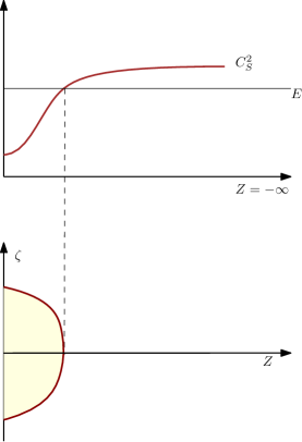
When the limiting velocity is minimal at the surface, that is,
| (46) |
there may still exist an eigenvalue of below . The corresponding eigenfunction exponentially decays “immediately” from the surface. This is somewhat different from the behavior of the eigenfunctions with eigenvalues above (See Figure 2). Here, we discuss the existence of such an eigenvalue.

For the principal symbol (cf. (35)) of , for , we have
and viewed as a polynomial in has non-real roots that appear in conjugate pairs. Suppose that are three roots with negative imaginary parts, and is a continuous curve enclosing . We let
| (47) |
where
| (48) |
and
with , for .
We define an operator,
| (49) |
A solution to in needs to satisfy
| (50) |
This follows from letting , and noting that . If for some , then
is exponentially growing as , since . This contradicts the fact that .
We now introduce the surface impedance tensor,
| (51) |
The basic properties of this tensor are summarized in
Proposition 5 ([20]).
For the following holds true
-
(i)
is Hermitian.
-
(ii)
is positive definite.
-
(iii)
The real part of is positive definite.
-
(iv)
At most one eigenvalue of is non-positive.
-
(v)
The derivative, , is negative definite.
-
(vi)
The limit exists.
To make this paper more self-contained, we include a proof of the above proposition. The properties of can be studied also by Stroh’s formalism and are important for the existence of subsonic Rayleigh wave in a homogeneous half-space; see [38] for a comprehensive overview.
Proof.
We use the Riccati equation
| (52) |
Taking the adjoint of , we find that
| (53) |
Subtracting from , we obtain
The above Sylvester equation is nonsingular, because and have disjoint spectra. Therefore
This proves (i).
Differentiating in , we get
The above Lyapunov-Sylvester equation has the unique solution
It is clear that is negative definite since . This proves (v).
In order to prove (ii), we assume that is a complex vector such that
Let
Then
We have the energy identity
By positivity of the differential operator, . Thus , and we have proved (ii).
With (47), (48) and (51), we obtain
where is the closed contour consisting of on the real line and the arc , , for large enough. We note that
We then have, by letting ,
The integral on the right-hand side is a real-valued matrix, and
is a positive definite matrix. Thus is positive definite. This proves (iii).
We prove (iv) by contradiction: Assume that has only one positive eigenvalue for some . The corresponding eigenspace would be one-dimensional. We can then choose a real-valued vector orthogonal to the eigenspace such that . This contradicts the fact that is positive definite, and proves (iv).
Finally, we prove (vi). Let be the operator norm of . Then is equal to the maximum of the absolute values of eigenvalues of . By (v), we have
Here , with Hermitian matrices and , means
for any complex vector . Thus the eigenvalues of are not greater than for . The sum of eigenvalues of is positive, since it is equal to , which is in turn equal to . Therefore, the possibly negative eigenvalue of is less than the sum of the two positive eigenvalues. Then
and we can take the limit in (vi). ∎
We now introduce the generalized Barnett-Lothe condition [28]: satisfies the generalized Barnett-Lothe condtion if
or
We note that in the isotropic case, this condition is satisfied for all .
We let be a solution of (50). Then the Neumann boundary value of is given by
The generalized Barnett-Lothe condition guarantees that has one negative eigenvalue. Therefore, with properties of established in Proposition 5, we have
Proposition 6.
There is a unique with such that , if the generalized Barnett-Lothe condition holds.
At the given in the proposition above, (50) has a solution that satisfies Neumann boundary condtion, that is, . We further assume . We emphasize, here, that the existence of such a depends on the stiffness tensor at boundary only. This locality behavior was first observed by Petrowsky [33].
We find that
by straightforward calculations, noting that
and
Then
since satisfies the Neumann boundary condition. Thus the
first eigenvalue of
satisfies
Therefore,
Theorem 7.
Assume that holds. If the generalized Barnett-Lothe condtion holds, and is sufficiently large, then there exists an eigenvalue of .
This particular eigenvalue may exist even when is constant (independent of ). It was first found by Rayleigh himself for the isotropic case. The uniqueness of such subsonic eigenvalue can be guaranteed if we further assume that is non-increasing as with respect to the order defined in the proof of Theorem 3.
5 Decoupling into Rayleigh and Love waves
5.1 Isotropic case
For the case of isotropy,
| (54) |
We introduce an orthogonal matrix
Using the substitution , with , we obtain the equations for the eigenfunctions,
| (55) |
| (56) |
for Love waves, and
| (57) |
| (58) |
| (59) | |||||
| (60) |
for Rayleigh waves. So we have two types of surface-wave modes, Love and Rayleigh waves, decoupled up to principal parts in an isotropic medium. The lower-order terms can be constructed following the proof of Theorem 1 leading to coupling.
5.2 Transversely isotropic case
We consider a transversely isotropic medium having the surface normal direction as symmetry axis. Then the nonzero components of are
and
Using the substitution , again, we obtain the equations for the eigenfunctions from :
| (61) |
| (62) |
for Love waves, and
| (63) |
| (64) |
| (65) | |||||
| (66) |
for Rayleigh waves.
5.3 Directional decoupling
We assume that , that is, the phase direction of propagation is , and assume that the medium is monoclinic with symmetry plane . Then is determined by 13 nonzero components:
The symmetry plane, , is called the sagittal plane. Then
We obtain the equations for the eigenfunctions:
| (67) | |||||
| (68) |
for Love waves, and
| (69) |
| (70) |
| (71) |
| (72) |
for Sloping-Rayleigh waves. We observe that the surface-wave modes decouple into Love waves and Sloping-Rayleigh waves when the direction of propagation is in the saggital plane.
For “global” decoupling, decoupling takes place in every direction of . Thus transverse isotropy is the minimum symmetry to obtain global decoupling; for a further discussion, see [1] . For more generally anisotropic media, decoupling is no longer possible. Then there only exist “generalized” surface-wave modes propagating with elliptical particle motion in three dimensions [14, 15]. Again, only in particular directions of saggital symmetry, however, the Sloping-Rayleigh and Love waves separate [16] up to the leading order term. This loss of polarization can be used to recognize anisotropy of the medium.
6 Weyl’s laws for surface waves
Weyl’s law was first established for an eigenvalue problems for the Laplace operator,
for a two- or three-dimensional bounded domain. One defines the counting function, , where are the eigenvalues arranged in a non-decreasing order with counting multiplicity. Weyl [41, 42, 43] proved the following behaviors,
| (73) |
for , and
| (74) |
for . Formulae of these type are referred to as Weyl’s laws. For a rectangular domain, one can easily find explicitly the eigenvalues and verify the formulae. These imply that the leading order asymptotics of the number of eigenvalues is determined by the area/volume of the domain only. Extensive work has been done generalizing this result and deriving expressions for the remainder term. We refer to [2] for a comprehensive overview. Here, we present Weyl’s laws for surface waves.
6.1 Isotropic case
Love waves
First, we consider the equations (55) and (56) for Love waves in isotropic media. We use the notation . We have the following Hamiltonian,
| (75) |
where is an ordinary differential operator in , with domain
We make use of results in [11]. Although in [11], the boundary condition is of Dirichlet type, the spectral property is essentially the same. A straightforward extension of the argument in [19] suffices:
where the point spectrum , consists of a finite set of eigenvalues in
and the continuous spectrum is given by
Since the problem at hand is scalar and one-dimensional, the eigenvalues are simple. We note that, here, the essential spectrum is purely the continuous spectrum.
We write , where is an eigenvalue of . Weyl’s law gives a quantitative asymptotic approximation of in terms of (Figure 3).
Theorem 8 (Weyl’s law for Love waves).
For any , we have
| (76) |
where denotes the measure of the set.
The classical Dirichlet-Neumann bracketing technique could be used to prove this theorem [35]. However, we can also adapt the proof of Theorem 9 below.
We observe that is a smooth function of for all . Moreover, the corresponding eigenfunctions, , decay exponentially in for large . More precisely, let , then for all , the corresponding are exponentially decaying from to . Hence, the energy of is concentrated near a neighborhood of . As , then the energy of with becomes more and more concentrated near the boundary. Thus those low-lying eigenvalues correspond to surface waves.
Remark 6.1.
For Love waves in a monoclinic medium described by equations , Weyl’s law reads: For any , we have
| (77) |
Rayleigh waves
Here, we establish Weyl’s law for Rayleigh waves, cf. (57)-(60). Now,
| (78) |
We use to denote the Fourier variable for . For fixed , we view as a semiclassical pseudodifferential operator with as semiclassical parameter, , as before. We denote . Then the principal symbol for is
There exists , namely,
such that
We write . We obtain
Theorem 9 (Weyl’s law for Rayleigh waves).
For any , define
where are the eigenvalues of . Then
| (79) |
Proof.
Let be real-valued, non-negative functions, such that for , for , and for some . For any non-negative , , is a trace class operator; we have
We analyze the two terms successively. We note that
and that is a pseudodifferential operator on with principal symbol,
Revisiting the diagonalization of above, let be the pseudodifferential operator with symbol
it follows immediately that is unitary on . Then
with being the pseudodifferential operator with symbol
Let and be the pseudodifferential operators with symbols and , respectively. Based on the discussion at the end of Appendix B,
| (80) |
We then observe that
where is the operator restricted to . To show this, we choose the eigenvalues, , and associated unit eigenvectors, , of subject to the Neumann boundary condition. Then forms an orthonormal basis of . We also consider an arbitrary orthonormal basis for . Clearly, form an orthonormal basis for . Therefore,
| (81) |
For every small , we can take , where is the indicator function of , that is,
Then
| (82) |
To show this, we rescale . Then for ,
| (83) |
where
| (84) |
on with the Neumann boundary condition applied. Without loss of generality, we can assume that is an integer. Then we divide the interval into intervals of the same length, , and let be operator restricted to , with the Neumann boundary condition applied. Then, as in the proof of Theorem 3,
The number of eigenvalues of each below can be bounded by a constant since the corresponding quadratic forms have a uniform lower bound. Hence, we obtain (82).
Using a technique similar to the one used in the proof of [45, Theorem 14.11], we construct by regularizing , with , such that
More presicely, we may take
where is chosen so that . Let , and
While observing that , and using the estimates above, taking completes the proof. ∎
6.2 Anisotropic case
We extend Weyl’s law from isotropic to anisotropic media. The proof for Rayleigh waves can be naturally adapted. We write the eigenvalues of the symmetric matrix-valued symbol defined in (35) as , and
Theorem 10.
Assume the three eigenvalues are smooth in , then for any , let
Then
7 Surface waves as normal modes
In this section, we identify surface wave modes with normal modes. We consider the Earth as a unit ball . There is a global diffeomophism, , with
where is the unit sphere centered at the origin. For an open and bounded subset , the cone region, , is diffeomorphic to ; hence, we can find global coordinates for and we may consider our system on the domain . More generally, we consider the system on any Riemannian manifold of the form with metric
Thus is a compact Riemannian manifold with metric . For a “nice” domain , a neighborhood of the boundary is diffeomorphic to , where the metric is the induced metric of the boundary of . We note that captures possible “topography” of (Figure 4).

Let be local coordinates on , and be local coordinates on . Then can be represented by
We represent on in local coordinates, similarly as in . Now the displacement is a covariant vector,
| (86) |
Here, is the covariant derivative associated with . Normal modes can be viewed as solutions to the eigenvalue problem for
| (87) |
with Neumann boundary condition. In fact, (87) is asymptotically equivalent to
| (88) |
where is the pseudodifferential operator on defined in Theorem 1. By the estimates, , it follows that is elliptic implying that
Thus is compact, and hence the spectrum of is discrete.
Now, let be an eigenfrequency, then we construct asymptotic solutions of (88) of the form
| (89) |
Inserting this expression into (88), from the expansion, we find that
and
| (90) |
| (91) |
Here, and are defined similar to those defined in Section 2.3. Thus
will be an asymptotic solution of (87).
Remark 7.1 (Radial manifolds).
Under the assumption of transverse isotropy and lateral homogeneity, that is, fixing an , and using the normal coordinates at , we have (61)-(66) with . Then we can construct asymptotic modes. Now corresponds to , where is the Laplacian on . Then we consider the eigenvalue problem:
| (92) |
and
| (93) |
| (94) |
Then, if we have the eigenvalues and eigenfunctions of ,
and solutions for the system (61)-(66) with , we find
as the solutions to (92)-(94). In spherically symmetric models of the earth, and are the spherical harmonics.
Acknowledgements
M.V.d.H. gratefully acknowledges support from the Simons Foundation MATH + X program and National Science Foundation grant DMS-1559587. A.I. is grateful to Department of Computational and Applied Mathematics, Rice University for the hospitality during his stay where the part of research was carried out. G.N. was partially supported by Grant-in-Aid for Scientific Research (15K21766 and 15H05740) of the Japan Society for the Promotion of Science. J.Z. thanks Brian Kennett for invaluable discussions.
Appendix A Semiclassical pseudodifferential operators
Here, we give a summary of the basic definition and properties of semiclassical pseudodifferential operators which are used in the main text. Let be a symbol that is smooth in . We say that , with , if
with .
Let for , and for some small . One says that is asymptotic to and writes
if for any
We refer to as the principal symbol of . A semiclassical psudodifferential operator associated with is defined as follows
Definition 11.
Suppose that is a symbol. We define the semiclassical pseudodifferential operator,
| (A.1) |
for any , which is compactly supported.
We have the following mapping property: For any ,
for some constant . Here, is an arbitrary real number, and denotes the Sobolev space in with exponent .
If and are two symbols, then
with
We use the notation for the composition of two symbols: .
Definition 12.
We call a family of functions (distributions) admissible if there exist constants and such that
for any . We denote by the space of such families.
Definition 13.
The wavefront set of , denoted by , of an admissible family is the closed subset of which is defined as
if and only if , , such that
for close to . Here is the semiclassical Fourier transform:
Definition 14.
Let be an open set in . The space of microfunctions, , in is the quotient
Let be a symbol such that
Let be the solution to the Hamilton system,
We denote by the map such that . The map is called the Hamiltonian flow of . For each solving
where , we have is invariant under the Hamiltonian flow of .
Appendix B Operator theory
Definition 15.
Let be a Hilbert space, a dense subspace of , and be an unbounded linear operator defined on .
-
1.
The adjoint of is the operator whose domain is , where
and
-
2.
is called self-adjoint if and .
-
3.
is called symmetric if and for all .
Definition 16.
-
1.
Let be an unbounded self-adjoint operator densely defined on , with domain . The spectrum of is
-
2.
The set of all for which is injective and has dense range, but is not surjective, is called the continuous spectrum of , denoted by .
-
3.
If there exists a satisfying that , is called an eigenvalue of . The set of all eigenvalues is called the point spectrum of , denoted by .
-
4.
The discrete spectrum of is the set of eigenvalues of that have finite dimensional eigenspaces.
-
5.
The essential spectrum of is .
Theorem 17.
A number is in the essential spectrum of if and only if there exists a sequence in (called singular sequence or Weyl sequence) such that
-
1.
for all
-
2.
-
3.
-
4.
Quadratic form. A quadratic form is a map , where is a dense linear subset of Hilbert space , such that is linear and is skew-linear. If we say that is symmetric.
The map is called semi-bounded if for some . A semi-bounded quadratic form is called closed if is complete under the norm
If is a closed semi-bounded quadratic form, then is the quadratic form of a unique self-adjoint operator , such that , for any . Conversely, for any self-adjoint operator on , there exists a corresponding quadratic form . Then we denote . If is merely symmetric, let for any . We can complete under the inner product
to obtain a Hilbert space . Then extends to a closed quadratic form on (This is known as Friedrichs extension). We call the closure of .
Let , be two self-adjoint operators on Hilbert spaces and , with domains and . Then denote to be the operator on , with domain with . Now assume that and are nonnegative, and . We write if and only if
-
1.
.
-
2.
For any , .
Lemma 18.
If and are two self-adjoint operators, , then
where denotes the n-th eigenvalue of , counted with multiplicity.
Trace class. Let be a compact operator, then is a selfadjoint semidefinite compact operator, and hence it has a discrete spectrum,
We say that the nonnegative are singular values
of .
is said to be of trace class, if
Theorem 19.
Suppose that is of trace class on and is any orthonormal basis of , then
converges absolutely to a limit that is independent of the choice of orthonormal basis. The limit is called the trace of , denoted by .
Theorem 20.
Suppose that is of trace class on and is a bounded operator on , then and are of trace class on , and
Theorem 21.
If is an operator of trace class on , and
then
Let be a semiclassical pseudodifferential operator with scalar symbol , then
with
If is of trace class, an immediate implication of the theorem above is that
References
- [1] D. Anderson, Elastic wave propagation in layered anisotropic media, Journal of Geophysical Research 66, (1961) 2953-2963
- [2] W. Arendt, R. Nittka, W. Peter, F. Steiner, Weyl’s law: spectral properties of the Laplacian in mathematics and physics, in Mathematical Analysis of Evolution, Information and Complexity, W. Arendt and W. P. Schleich, eds., Wiley-VCH Verlag, Weinheim, Germany (2009).
- [3] V. Babich, B. Chikhachev, T. Yanovskaya, Surface waves in a vertically inhomogeneous elastic half space with weak horizontal inhomogeneity. Izv. Bull. Akad. Sci. USSR, Phys. Solid Earth 4 (1976) 24-31.1
- [4] C. Bardos, L. Boutet de Monvel, From the atomic hypothesis to microlocal analysis, notes, (2002)
- [5] F. Bretherton, Propagation in slowly varying waveguides. Proc. R. Soc. A 302 (1968) 555-576.
- [6] L. Brekhovskikh, Y. Lysanov, Fundamental of ocean acoustics. Springer-Verlag, Berlin, (1982).
- [7] J. Combes, P. Duclos, R. Seiler, Krein’s formula and one-dimensional multiple-well. J. Funct. Anal. 52, no. 2, (1983) 257-301.
- [8] J. Combes, P. Duclos, R. Seiler,Convergent expansions for tunneling, Comm. Math. Phys. 92, (1983) 229-245.
- [9] Y. Colin de Verdière, Elastic wave equation, Séminaire de théorie spectrale de géométire, GRENOBLE, 25, (2007) 55-69.
- [10] Y. Colin de Verdière. Mathematical models for passive imaging I: general background. arXiv:math-ph/0610043
- [11] Y. Colin de Verdière. Mathematical Models for passive imaging II: Effective Hamiltonians associated to surface waves. arXiv:math-ph/0610044
- [12] Y. Colin de Verdière. Semiclassical analysis and passive imaging. Nonlinearity 22, no. 6(2009), R45–R75.
- [13] Y. Colin de Verdière. A semi-classical inverse problem II: reconstruction of the potential, Geometric Aspects of Analysis and Mechanics: In Honor of the 65th Birthday of Hans Duistermaat, (Eds) J. A. C. Kolk and Erik P. van de Ban, Birkhäuser, Boston, MA (2011) 97-119 .
- [14] S. Crampin, The dispersion of surface waves in multi-layered anisotropic media, Geopyhs. J. R. Astr. Soc. 21 (1970), 387-402
- [15] S. Crampin, Distinctive particle motion of surface waves as a diagnostic of anisotropic layering, Geophys. J. R. astr. Soc., 40 (1975), 177-186.
- [16] S. Crampin, A review of wave motion in anisotropic and cracked elastic-media, Wave Motion 3 (1981), 343-391.
- [17] F. Dahlen, J. Tromp, Theoretical global seismology, Princeton University Press, 1998.
- [18] M. Dimassi, J. Sjöstrand, Spectral asymptotics in the semi-classical limit. London Mathematical Society Lecture Note Series, 268. Cambridge University Press, Cambridge, (1999).
- [19] G. Gladwell The Schrödinger Equation on the Half Line. Inverse Problems in Scattering Solid Mechanics and its Applications 23, (1993), 251–287.
- [20] S. Hansen, Subsonic free surface waves in linear elasticity, Siam J. Math. Anal., 46 (2014), pp. 2501-2524.
- [21] B. Helffer, J. Sjöstrand, Multiple wells in the semiclassical limit. I. Comm. Partial Differential Equations, 9, no.4, (1984), 295-308.
- [22] I. Kamotskii, A. Kiselev, An energy approach to the proof of the existence of Rayleigh waves in an anisotropic elastic half-space, J. Appl. Math. and Mech., 73, (2009), 464-470.
- [23] A. Love, Some problems of geodynamics. Cambridge University Press reprinted by Dover Publications, (1967), New York.
- [24] P. Malischewsky, Surface waves and discontinuities. Akademie Verlag, Berlin, 1987
- [25] C Man, G. Nakamura, K. Tanuma, Dispersion of the Rayleigh wave in vertically-inhomogeneous prestressed elastic media, IMA J. Appl. Math 80 (2015), 47-84.
- [26] A. Martinez, An introduction to semiclassical and microlocal analysis. Universitext. Springer-Verlag, New York, 2002.
- [27] A. Mielke, Y. Fu., Uniqueness of the surface-wave solutions for anisotropic half-spaces with free surface, J. Appl. Phys., 47 (1976), pp. 428-433.
- [28] G. Nakamura, Existence and Propagation of Rayleigh waves and pulses, Modern Theory of Anisotropic Elasticity and Applications, SIAM Proceedings, (1991), 215-231.
- [29] G. Nakamura, G. Uhlmann, A layer stripping algorithm in elastic impedance tomography. IMA Vol. Math. Appl., 90, Springer, New York, (1997), 375-384.
- [30] V. E. Nomofilov, Propagation of quasielastic Rayleigh waves in and inhomogeneous, anisotropic, elastic medium, Zap. Naucha, Sem. Lenigr. Otd. Mat. Inst. 89 (1979), 234-245.
- [31] R. Odom, A coupled mode examination of irregular waveguides including the continuous spectrum. Geophys. J. Roy. Astron. Soc. 86 (1986), 425-453.
- [32] A. Pandov. Introduction to Spectral Theory of Schrödinger Operators. www.math.nsysu.edu.twamenposterspankov.pdf
- [33] I. Petrowsky, On the propagation velocity of discontinuities of the displacement derivatives on the surface of an inhomogeneous elastic body of arbitrary form. C. R. (Doklady) Acad. Sci. URSS (N. S.), 47, 255-258.
- [34] J. Rayleigh, On waves propagated along the plane of an elastic solid. Proc. Lond. Math. Soc. 17 (1885) 4-11.
- [35] M. Reed, B. Simon, Methods of Modern Mathematical Physics, I-IV, Academic, (1980).
- [36] P. Shearer, Introduction to seismology, 2nd edition, Cambridge University Press, (2009).
- [37] B. Simon, Semiclassical analysis of low lying eigenvalues. I. Nondegenerate minima: asymptotic expansions. Ann. Inst. H. Poincaré Sect. A (N.S.) 38, no.3., (1983), 295-308.
- [38] K. Tanuma, Stroh formalism and Rayleigh waves, Journal of Elasticity 89, (2007), 5-154.
- [39] S. Teufel, Adiabatic perturbation theory in quantum mechanics. Lecture notes in Mathematics, Vol. 1821. Springer Verlag, (2003).
- [40] J. Tromp, F. Dahlen, Variational principles for surface wave propagation on a laterally heterogeneous Earth -I. Time-domain JWKB theory. Geophys. J. Int. 109 (1992) 581-598.
- [41] H. Weyl, Über die Abhäangigkeit der Eigenschwingungen einer Menbran von deren Begrenzung, J. Reien Angew. Math.141, (1912), 1-11.
- [42] H. Weyl, Über das Spektrum der Hohlraunmstrahlung, J. Reien Angew. Math. 141, (1912), 163-181.
- [43] H. Weyl, Über die Randwertaufgabe der Strahlungstheorie und asymptotische Spectralgeometrie, J. Reien Angew. Math. 143, (1913), 177-202.
- [44] J. Woodhouse, Surface waves in a laterally varying layered structure. Geophys. J. Roy. Astron. Soc. 37 (1974) 461-490.
- [45] M. Zworski, Semiclassical analysis. AMS Graduate Studies in Mathematics. Vol 138. (2012)