Cosmic-ray Antimatter

Abstract

In recent years, space-born experiments have delivered new measurements of high energy cosmic-ray (CR) $\bar{p}$ and $e^{+}$. In addition, unprecedented sensitivity to CR composite anti-nuclei $\rm\bar{d}$ and $\overline{\rm{}^{3}He}$ is expected to be achieved in the near future. We report on the theoretical interpretation of these measurements. While CR antimatter is a promising discovery tool for new physics or exotic astrophysical phenomena, an irreducible background arises from secondary production by primary CR collisions with interstellar matter. Understanding this irreducible background or constraining it from first principles is an interesting challenge. We review the attempt to obtain such understanding and apply it to CR $\bar{p},\,e^{+},\,\rm\bar{d},$ and $\overline{\rm{}^{3}He}$.

Based on state of the art Galactic cosmic ray measurements, dominated currently by the AMS-02 experiment, we show that: (i) CR $\bar{p}$ most likely come from CR-gas collisions; (ii) $e^{+}$ data is consistent with, and suggestive of the same secondary astrophysical production mechanism responsible for $\bar{p}$ and dominated by proton-proton collisions. In addition, based on recent accelerator analyses we show that the flux of secondary high energy $\overline{\rm{}^{3}He}$ may be observable with a few years exposure of AMS-02. We highlight key open questions, as well as the role played by recent and upcoming space and accelerator data in clarifying the origins of CR antimatter.

I Introduction

Cosmic ray (CR) physics is centred on the attempt to solve a set of basic open questions Ginzburg and Ptuskin (1976); Ginzburg et al. (1990). Where do CRs come from, namely, what are the sources of the bulk of the CR energy density? where are these sources located, and how do they accelerate particles? Narrowing to the Galactic energy range ($\sim$MeV to at least $\sim$PeV per particle): what role do CRs play in Galactic dynamics? How do CRs propagate and eventually escape from the Galaxy? Where and how does the transition to extra-galactic sources occur?

From this wide perspective CR antimatter is an exotic phenomena, making an insignificant contribution to the total CR energy density (in the ballpark of 0.01 percent). Nevertheless, careful study of CR antimatter may reveal important insights to CR physics and beyond that, particle physics. Because considerable energy is required to create antimatter, it is a valuable probe of high energy processes. Because primordial antimatter is essentially absent before structure formation, its formation as secondary product in CR collisions with ambient gas makes the description of CR antimatter theoretically clean, decoupling the problem – to some extent – from core unknowns in the physics of CR sources and acceleration.

As a result, one is led to a situation where although the sources of the bulk of the Galactic CRs – primary protons, He, and other nuclei – are essentially not understood, nevertheless the small residual accompanying radiation of $\bar{p}$, essentially is. Using this theory control, spectral features or excess abundance of CR antimatter could lead to a first detection of exotic phenomena like dark matter annihilation or $e^{\pm}$ pair-production in pulsars. In addition, antimatter provides a unique handle on the physics of CR propagation.

In this review we discuss CR antimatter. Aiming to jump directly to what we consider new and exciting developments, we leave out most of the basic CR physics background; as a partial list of useful books we recommend Ginzburg et al. (1990); Longair (1992); Kulsrud (2005); Gaisser et al. ; Schlickeiser (2002). Review papers are referred to where relevant. We attempt to avoid astrophysics modelling assumptions as much as possible. This is not an easy task, as much of the CR literature is focused on phenomenological modelling of propagation. We leave out most of the modelling questions, hoping to provide a simple and robust understanding of CR antimatter that would be beneficial to particle physicists and astrophysicists alike.

Our work is motivated by new observational information coming from an array of experiments. Focusing on recent CR antimatter and closely related results we note, as a partial list of experimental contributions, the $e^{\pm}$ and $\bar{p}$ measurements of PAMELA Adriani et al. (2009, 2010); Adriani et al. (2013a), FERMI Abdo et al. (2009); Ackermann et al. (2012a); Ackermann et al. (2010), ATIC Chang et al. (2008), HESS Aharonian et al. (2008, 2009), and AMS02 Aguilar et al. (2013, 2016a); Ting . Future results are expected from CALET Marrocchesi (2016), DAMPE Wang et al. (2016) and CTA Vandenbroucke et al. (2016). Progress in the search for $\rm\bar{d}$ and $\overline{\rm{}^{3}He}$ is expected with AMS02 Giovacchini and Choutko (2007); Kounine , GAPS von Doetinchem et al. (2016); Aramaki et al. (2016a), and BESS Abe et al. (2012, 2012).

The layout of this review is as follows. In Sec. II we consider secondary $\bar{p}$ – from the theoretical perspective, the simplest form of CR antimatter. In Sec. II.1-II.2 we show how stable, relativistic, secondary nuclei data, under the general assumption that the CR elemental composition is approximately uniform in the regions dominating spallation, allow one to calibrate away most of the propagation modelling uncertainties and extract a parameter-free prediction for $\bar{p}$. The same calibration process is known to describe well the fluxes of secondary CR nuclei. For $\bar{p}$, residual sensitivity remains to possible CR spectral variations in the spallation regions, as we discuss at some length. The insight behind this calibration process and a discussion of the conditions for its validity are presented in App. A. We find the secondary $\bar{p}$ prediction to be consistent with data within the uncertainties. In Sec. II.3 we compare the model-independent analysis with certain models of propagation.

In Sec. III we turn to $e^{+}$, a hot potato: here public opinion basically has it that a primary source of $e^{+}$ must exist, be it dark matter or pulsars. We take a fresh look at the data in Sec. III.1; the first thing we notice appears like a hint in the opposite direction: the observed $e^{+}/\bar{p}$ flux ratio saturates the ratio of production rates in proton-proton collisions, a compelling hint for secondary $e^{+}$. We devote Sec. III.2 to elucidate the picture for $e^{+}$. If $e^{+}$ are secondary, then $e^{+}$ energy losses during propagation must be small, requiring that the CR propagation time is shorter than the time scale it takes $e^{+}$ to radiate a significant amount of their energy. Such a scenario cannot be accommodated in the conventional CR diffusion models Strong et al. (2007), and this inconsistency with propagation models was the main cause for the claim of an “$e^{+}$ anomaly” Adriani et al. (2009). To be clear: we do not know of a fully satisfactory and tested alternative propagation model that reproduces the behaviour of $e^{+}$ with secondary production. However, putting modelling questions aside, we show in Sec. III.3 that high energy radioactive nuclei data could test the secondary $e^{+}$ hypothesis in the near future. In Sec. III.4 we provisionally assume that $e^{+}$ are secondary to review some general lessons for CR propagation. These lessons which, again, are in tension with the currently common models of CR diffusion, may yet prove to be the long-term legacy of today’s state of the art Galactic CR experiments. In Sec. III.5 we review some CR propagation models for secondary $e^{+}$. Finally, in Sec. III.6 we review ideas for primary $e^{+}$ or $\bar{p}$ from pulsars and dark matter annihilation, showing that these models generically invoke fine-tuning to reproduce the observations.

In Sec. IV we tackle the topic of CR $\rm\bar{d}$ and $\overline{\rm{}^{3}He}$. Surprisingly enough, we find a hot potato also here: we suggest, contrary to most earlier estimates, that a detection of secondary $\overline{\rm{}^{3}He}$ may be imminent at AMS02 (consistent with some pesky recent rumours).

In Sec. V we conclude. A short technical discussion of the interplay between $e^{+}$ radiative losses and propagation time is reserved to App. B.

II Astrophysical $\bar{p}$: the Galaxy as a fixed-target experiment

CR antimatter particles are produced as secondaries in collisions of other CRs, notably protons, with interstellar matter (ISM), notably hydrogen in the Galaxy. Highly relativistic $\bar{p}$ and heavier antinuclei ($\rm\bar{d},\,\overline{\rm{}^{3}He}$) propagate similarly to relativistic matter nuclei at the same magnetic rigidity

$$\mathcal{R}=p/eZ,$$

with the difference in charge sign expected to make little or no impact on the propagation given that the measured CR flux is very nearly locally isotropic Di Sciascio and Iuppa (2014).

Starting with the simplest case of $\bar{p}$, it is natural to try and calibrate the effect of propagation directly from data, by using information on other secondary nuclei like boron (B), formed by fragmentation of heavier CRs (mostly carbon C and oxygen O). We now explain how to perform this calibration, calculate the predicted $\bar{p}$ flux, and compare to measurements.

II.1 The CR grammage

In this section we limit the discussion to stable, relativistic, secondary nuclei. For such secondaries, including e.g. B and the sub-Fe group (T-Sc-V-Cr), the ratio of densities of two species $a,b$ satisfies an approximate empirical relation Engelmann et al. (1990); Webber et al. (2003),

$$\frac{n_{a}(\mathcal{R})}{n_{b}(\mathcal{R})} \approx \frac{Q_{a}(\mathcal{R})}{Q_{b}(\mathcal{R})}.$$ (1)

Here $Q_{a}$ denotes the net production of species $a$ per unit ISM column density,

$$Q_{a}(\mathcal{R}) = \sum_{P}n_{P}(\mathcal{R})\frac{\sigma_{P\to a}(\mathcal{R})}{m}-n_{a}(\mathcal{R})\frac{\sigma_{a}(\mathcal{R})}{m},$$ (2)

where $(\sigma_{a}/m)$ and $(\sigma_{P\to a}/m)$ are the total inelastic and the partial $P\to a$ cross section per target ISM particle mass $m$, respectively.

We stress that Eq. (1) is an empirical relation, known to apply to $\sim$10% accuracy in analyses of HEAO3 data Engelmann et al. (1990); Webber et al. (2003) and – as we shall see shortly, focusing on $\bar{p}$ – consistent with subsequent PAMELA Adriani et al. (2013a) and AMS02 Aguilar et al. (2016a) measurements. In applying Eq. (1) to $\bar{p}$, a subtlety arises due to the fact that the cross sections appearing in Eq. (2) can (and for $\bar{p}$, do) depend on energy. In Eq. (2) we define these cross sections such that the source term $Q_{a}(\mathcal{R})$ is proportional to the progenitor species density $n_{P}(\mathcal{R})$ expressed at the same rigidity; we will clarify this statement further down the road in Eq. (6). For relativistic nuclei (above a few GeV/nuc) produced in fragmentation reactions, e.g. ¹²C fragmenting to ¹¹B, the energy dependence of the fragmentation cross section is much less important.

From the theoretical point of view, Eq. (1) is natural Katz et al. (2010); Ptuskin et al. (1996); Stephens and Streitmatter (1998); Ginzburg et al. (1990). It is guaranteed to apply if the relative elemental composition of the CRs in the regions that dominate the spallation is similar to that measured locally at the solar system: in this case, the source distribution of different secondaries is similar. Because the confinement of CRs in the Galaxy is magnetic, different CR particles that share a common distribution of sources should exhibit similar propagation if sampled at the same rigidity. Thus, the ratio of propagated CR densities reflects the ratio of their net production rates.

Note that the net source defined in Eq. (2) accounts for the fact that different nuclei exhibit different degree of fragmentation losses during propagation. In this way, species like sub-Fe (with fragmentation loss cross section of order 500 mb), B ($\sigma_{B}\sim 240$ mb), and $\bar{p}$ ($\sigma_{\bar{p}}\sim 40$ mb) can be put on equal footing.

Further discussion of the physical significance of Eq. (1) is given in Ref. Katz et al. (2010) and App. A.

We can use Eq. (1) together with the locally measured flux of B, C, O, p, He,… to predict the $\bar{p}$ flux Gaisser and Schaefer (1992); Katz et al. (2010):

$$n_{\bar{p}}(\mathcal{R}) \approx \frac{n_{\rm B}(\mathcal{R})}{Q_{\rm B}(\mathcal{R})}Q_{\bar{p}}(\mathcal{R}).$$ (3)

The RHS of Eq. (3) is derived from laboratory cross section data and from direct local measurements of CR densities, without reference to the details of propagation.

The quantity

$$X_{\rm esc}(\mathcal{R}) = \frac{n_{\rm B}(\mathcal{R})}{Q_{\rm B}(\mathcal{R})},$$ (4)

known as the CR grammage Ginzburg et al. (1990), is a spallation-weighted average of the column density of ISM traversed by CRs during their propagation, the average being taken over the ensemble of propagation paths from the CR production regions to Earth. Combining AMS02 B/C Aguilar et al. (2016b) and C/O Ting with heavier CR data from HEAO3 Engelmann et al. (1990) and with laboratory fragmentation cross section data Blum et al. (2017a); Tomassetti (2015), one can derive $X_{\rm esc}$ directly from measurements:

$$X_{\rm esc} = \frac{\rm(B/C)}{\sum_{\rm P=C,N,O,...}{\rm(P/C)}\frac{\sigma_{\rm P\to B}}{m}-{\rm(B/C)}\frac{\sigma_{\rm B}}{m}}.$$ (5)

The result for $X_{\rm esc}$ is shown by the green markers in the left panel of Fig. 1. Error bars reflect the B/C error bars reported in Aguilar et al. (2016b), and do not include systematic uncertainties on fragmentation cross sections and on the flux ratios C/O, N/O, etc. We estimate that the systematic fragmentation cross section uncertainties are at the level of 20%; note that many of the cross sections used in the analysis at high energy are extrapolated from much lower energy data, typically confined to a few GeV/nuc. The result in Fig. 1 agrees with the power-law approximation derived in Ref. Blum et al. (2013) to 20% accuracy.

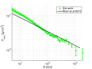
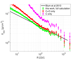
Figure 1: Left: CR grammage $X_{\rm esc}$ derived directly from B/C, C/O, and heavier nuclei data and compared with the earlier approximation of Blum et al. (2013). Right: separating various contributions to the full $X_{\rm esc}$ result. Error bars represent only the B/C error bars reported in Aguilar et al. (2016b), and do not include systematic uncertainties on fragmentation cross sections and on the flux ratios.

To exhibit the different contributions entering the determination of $X_{\rm esc}$, in the right panel of Fig. 1 we show the result for $X_{\rm esc}$ that obtains if we omit, in the B production source, the contributions due to all CR species other than C (purple markers), all species other than C+O (red markers).

II.2 $\bar{p}/p$ from B/C

Now that we have $X_{\rm esc}$, we can use the $\bar{p}$ production and loss cross sections parametrised in, e.g., Tan and Ng (1983, 1983); Winkler (2017) together with measurements of the proton and helium Aguilar et al. (2015a, b); Yoon et al. (2017) flux to calculate $Q_{\bar{p}}$ and apply it in Eq. (3). At low rigidity, the effect of solar modulation is estimated as in Webber et al. (2003) with $\Phi=450$ MV.

The result is compared to AMS02 data Aguilar et al. (2016a); Nozzoli (2016) in Fig. 2. The $\bar{p}$ flux is consistent, within statistical and systematic uncertainties, with the prediction of Eq. (3). No astrophysical propagation modelling is needed: Eq. (3) has successfully calibrated out propagation from B/C data.

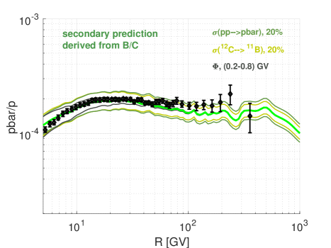
Figure 2: Observed $\bar{p}/p$ ratio Aguilar et al. (2016a) vs. the secondary prediction, calculated using the locally measured B/C ratio and p and He flux. Wiggles in the theory curve come from our direct data-driven use of the CR grammage, and reflect fluctuations in the AMS02 B/C data Aguilar et al. (2016b). Thick line is the secondary prediction with input cross sections detailed in Blum et al. (2017a), while thin lines show the response of the prediction for variation in (i) $pp\to\bar{p}$ cross section within $\pm 20\%$, (ii) fragmentation cross section p¹²C$\to$¹¹B within $\pm 20\%$, (iii) variation in the solar modulation parameter in the range $\Phi=(0.2-0.8)$ GV. Taken from Ref. Blum et al. (2017a).

We can conclude that CR $\bar{p}$ are most likely secondary.

As mentioned earlier, in computing $Q_{\bar{p}}$ we need to account for the energy-dependent $\bar{p}$ production cross section. Let us consider the main positive contribution to $Q_{\bar{p}}$, due to pp collisions. Because of a kinematical barrier, the daughter $\bar{p}$ is emitted with a rigidity smaller by a factor of $\sim 10$ compared to the rigidity of the parent $p$ in the ISM frame. Given a spectrum of parent protons, one can still compute the overlap integral between the differential cross section and the parent p spectrum and express the contribution to $Q_{\bar{p}}$ in terms of an effective cross section $\sigma_{p\to\bar{p}}(\mathcal{R})$:

$$\sigma_{p\to\bar{p}}(\mathcal{R}) = \frac{2\int_{\mathcal{R}}^{\infty}d\mathcal{R}_{p}\,J_{p}(\mathcal{R}_{p})\left(\frac{d\sigma_{pp\to\bar{p}X}(\mathcal{R}_{p},\mathcal{R})}{d\mathcal{R}_{p}}\right)}{J_{p}(\mathcal{R})}.$$ (6)

The factor of 2 above accounts for the production and subsequent decay of $\bar{n}$, with $\sigma_{pp\to\bar{n}X}\approx\sigma_{pp\to\bar{p}X}$. A similar procedure is used to include the contributions due to proton CR hitting He in the ISM; He CR hitting ISM hydrogen; and so forth.

Calculating Eq. (6) for a power-law proton flux $J_{p}\propto\mathcal{R}^{-\gamma_{p}+\Delta\gamma_{p}}$, one finds the scaling $\sigma_{p\to\bar{p}}^{(\Delta\gamma_{p})}\approx 10^{\Delta\gamma_{p}}\,\sigma_{p\to\bar{p}}^{(\Delta\gamma_{p}=0)}$ Katz et al. (2010). The effective cross section $\sigma_{p\to\bar{p}}(\mathcal{R})$ therefore depends on the spectral shape of CR protons. This is a new feature compared to the heavy nuclei fragmentation cross sections: there, due to the straight-ahead kinematics, a cross section like $\sigma_{\rm C\to B}$ is independent of the carbon spectral index to a good approximation.

Calculating $\sigma_{p\to\bar{p}}(\mathcal{R})$ with the locally measured p flux, one might expect deviations from Eq. (1) if the proton spectral shape in the spallation regions exhibits variations compared to its locally measured value. Models that realise this possibility include Cowsik and Burch (2009); Burch and Cowsik (2010); Cowsik et al. (2014); Blasi (2009); Blasi and Serpico (2009); Mertsch and Sarkar (2009); Ahlers et al. (2009); Kachelriess et al. (2011); Cholis et al. (2017); Kachelrie et al. (2015); Thomas et al. (2016), reviewed in Sec. III.5.

In Fig. 3 we quantify the sensitivity of the locally measured $\bar{p}/p$ ratio to a difference between the primary CR spectrum measured locally, to the spectrum in the regions of the Galaxy that dominate the secondary production. Similarly, the plot also exhibits the sensitivity in the predicted $\bar{p}/p$ ratio to measurement errors in determining the local proton flux. We show the $\bar{p}/p$ ratio that obtains if, in the calculation of $\sigma_{p\to\bar{p}}(\mathcal{R})$, we replace the locally measured proton flux by a modified spectrum: $J_{p}(\mathcal{R})\to J_{p}(\mathcal{R})F_{p}(\mathcal{R})$, with $F_{P}(\mathcal{R})=1$ for $\mathcal{R}\leq 200$ GV and $F_{p}(\mathcal{R})=\left(\mathcal{R}/{\rm 200~{}GV}\right)^{\Delta\gamma_{p}}$ for $\mathcal{R}>200$ GV. The result is shown for the choices $\Delta\gamma_{p}=-0.15,\,0,\,0.15,\,0.3,\,0.5$. Note that our parametrization of the locally measured proton flux uses a direct (non power-law) interpolation of AMS02 Aguilar et al. (2015a) and CRAM-III Yoon et al. (2017) data.

Allowing room for cross section and CR spectra uncertainties, from inspection of Fig. 3 we infer a rough limit:

$$-0.15<\Delta\gamma_{p}<0.4.$$ (7)

Eq. (7) applies to the situation where all primary CR spectra are modified in the secondary production regions, compared to their local value; namely, the variation in proton and in C and O spectra is correlated, $\Delta\gamma_{\rm C,O}\approx\Delta\gamma_{p}$. This could occur with nontrivial propagation from the CR fragmentation regions to our local spot in the Milky Way. One may also constrain the possibility of CR accelerators that inject a different composition of primary CR spectra in different (but connected by propagation) regions of the Galaxy, in which case $\Delta\gamma_{\rm C,O}\neq\Delta\gamma_{p}$. This situation corresponds to significantly non-uniform CR composition in the propagation region, invalidating the grammage relation. While we do not pursue this analysis here, it is also constrained by the success of Eq. (3) in reproducing the $\bar{p}/p$ data.

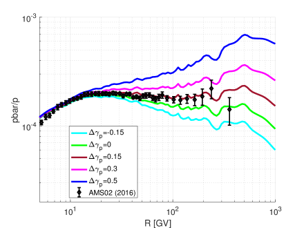
Figure 3: Same as Fig. 2, but showing in cyan, green, red, magenta, and blue the resulting local value of $\bar{p}/p$ that obtains if the high energy proton spectrum in the spallation region is changed w.r.t. the locally measured spectrum by a factor $\left(\mathcal{R}/200~{}{\rm GV}\right)^{\Delta\gamma_{p}}$, starting at $\mathcal{R}>200$ GV, with $\Delta\gamma_{p}=-0.15,\,0,\,0.15,\,0.3,\,0.5$, respectively.

To conclude so far:

• When it comes to relativistic, stable, secondary nuclei and antinuclei, the Galaxy is essentially a fixed-target experiment, with CRs themselves playing the role of the beam and with ISM being the target. This simple point and the resulting predictions are often obscured in calculations done within specific models of CR propagation.

• Fig. 2 demonstrates that the $\bar{p}$ flux measured by AMS02 Aguilar et al. (2016a) is consistent with secondary production, within current fragmentation and $pp\to\bar{p}$ cross section uncertainties and the uncertainties in B/C and primary CR spectra.

It is worthwhile to compare our analysis to results obtained in the context of specific models of propagation. Of these, the most commonly used are the two-zone disc+halo diffusion models Strong et al. (2007). In the next section we discuss these models in view of the $\bar{p}$ data.

II.3 $\bar{p}$ in diffusion models

Typical two-zone diffusion models in the literature satisfy the simple condition leading to Eq. (1), so they too satisfy Eq. (1), at least approximately Ginzburg et al. (1990). This is because the relative composition of the CRs in these models is approximately uniform across the thin ISM disc, where most of the spallation happens. It is interesting to compare results obtained within these models to results derived directly from Eq. (1).

A recent example of the diffusion model was given in Kappl et al. (2015); Winkler (2017). Ref. Kappl et al. (2015); Winkler (2017) calibrated the diffusion model to AMS02 B/C data, and used the resulting model parameters together with state of the art proton and He data to calculate the $\bar{p}$ flux. The result, taken from Winkler (2017), is shown by the blue line in Fig. 4. As can be seen, this result is consistent with the result obtained directly from Eq. (1), using the same B/C, p and He data and a similar $pp\to\bar{p}$ cross section code.

As another example, Ref. Donato et al. (2009) used a diffusion model with the same set of assumptions, geometry, and free parameters to that of Kappl et al. (2015); Winkler (2017). However, the $\bar{p}/p$ ratio predicted in Donato et al. (2009), shown by the yellow band in Fig. 4, falls significantly below the AMS02 $\bar{p}/p$ data. What went wrong?

The main thing that went wrong, is that the model of Ref. Donato et al. (2009) was calibrated to fit early B/C data from HEAO3 Engelmann et al. (1990), and then extrapolated from that fit to high energy beyond the region where HEAO3 data was tested. Unfortunately, above $\mathcal{R}\sim 100$ GV the extrapolation of the HEAO3 B/C data falls bellow the more recent AMS02 measurement. In addition, Donato et al. (2009) assumed a primary proton flux with high energy spectral index $\gamma_{p}=2.84$, softer by about $\Delta\gamma_{p}\approx-0.12$ than the proton flux seen by AMS02. The implications of this soft high energy proton spectrum can be estimated from Fig. 3. At the same time, at lower energy $\mathcal{R}\lesssim 100$ GV the assumed proton flux was higher than that reported by AMS02, decreasing further the predicted $\bar{p}/p$ ratio.

As a result, Ref. Donato et al. (2009) predicted a low $\bar{p}/p$ ratio. To illustrate this fact, we show in Fig. 4 by a red line the result we find if we calculate the $\bar{p}/p$ ratio using Eq. (1), but using the value of $X_{\rm esc}$ derived for the diffusion model of Donato et al. (2009) with $\delta=0.7$ and using the same proton flux assumed there. The discrepancy with Ref. Donato et al. (2009) is reproduced.

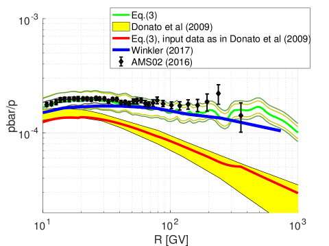
Figure 4: Comparison of the result of Eq. (3) (green) with results from the diffusion models of Winkler (2017) (blue) and Donato et al. (2009) (yellow band). AMS02 data in black. To understand the discrepancy with Donato et al. (2009), we use the model parameters of Ref. Donato et al. (2009), based on early HEAO3 B/C data, to compute the effective $X_{\rm esc}$. We then use this $X_{\rm esc}$ to calculate the $\bar{p}$ flux. We also adopt the primary p and He spectra and $pp\to\bar{p}$ cross section parametrisation of Donato et al. (2009). The result we obtain in this way is shown in red.

III What is the issue with $e^{+}$?

Measurements of the positron fraction $e^{+}/e^{\pm}=e^{+}/(e^{+}+e^{-})$ by the PAMELA Adriani et al. (2009, 2010) and AMS02 Aguilar et al. (2013) experiments have shown that $e^{+}/e^{\pm}$ is rising with energy from a few GeV to at least 300 GeV. This trend of rising $e^{+}/e^{\pm}$ was claimed by many to indicate a primary source dominating the $e^{+}$ flux at these energies. Understanding the true story behind CR $e^{+}$ is crucial: models for a primary source range from dark matter annihilation to a contribution of $e^{\pm}$ from pulsars, both exciting ideas.

Our goal in this section is to consider what can be learned from the $e^{+}$ measurements. We start with inspecting the data, in Sec. III.1, pointing out that the observed $e^{+}/\bar{p}$ flux ratio saturates the ratio of production rates $Q_{e^{+}}/Q_{\bar{p}}$ in proton-proton collisions. This is a compelling hint for secondary $e^{+}$.

What then is the basis to the claim that a primary $e^{+}$ source is required? In Sec. III.2 we show that if $e^{+}$ are secondary, then $e^{+}$ energy losses during propagation must be small, requiring that the CR propagation time is shorter than the time scale it takes $e^{+}$ to radiate a significant amount of their initial energy (of order $\sim 1$ Myr at $\mathcal{R}\sim 300$ GV). Such a scenario cannot be accommodated in the conventional phenomenological diffusion models Strong et al. (2007), and the inconsistency with propagation models was the main cause for the claim of an “$e^{+}$ anomaly” Adriani et al. (2009). However, we know of no contradiction of this scenario with either observational data or first principle theory.

The nearest complimentary data that could test the secondary $e^{+}$ hypothesis involves radioactive secondary nuclei, and we review it in Sec. III.3. In Sec. III.4 we entertain the possibility that $e^{+}$ are indeed secondary, and deduce some basic model-independent lessons for CR astrophysics. In Sec. III.5 we review some CR propagation models for secondary $e^{+}$. Finally, in Sec. III.6 we review ideas for primary $e^{+}$ or $\bar{p}$ from pulsars and dark matter annihilation, showing that these models generically invoke fine-tuning to reproduce the observations.

III.1 A hint for secondary $e^{+}$

In dealing with $\bar{p}$ we used Eq. (1), cast in the form of Eq. (3) where $X_{\rm esc}=n_{B}/Q_{B}$ is derived from nuclei data. However, Eq. (1) cannot be directly applied to predict the flux of $e^{+}$, because $e^{+}$ are subject to radiative energy losses and Eq. (1) does not capture the effect of energy loss during propagation (see discussion in App. A).

Nevertheless, we can still gain insight from Eq. (1). As noted in Katz et al. (2010), Eq. (1), applied to $e^{+}$ with radiative losses ignored, provides an upper limit to the secondary $e^{+}$ flux because radiative energy losses can only decrease the secondary $e^{+}$ flux compared to the loss-less secondary benchmark. This provides an upper bound on the flux of secondary $e^{+}$.

The most robust way to formulate the secondary upper bound on the $e^{+}$ flux is in terms of branching fractions in pp collisions, comparing $e^{+}$ to $\bar{p}$. The upper bound reads:

$$\frac{n_{e^{+}}}{n_{\bar{p}}} \leq \frac{Q_{e^{+}}(\mathcal{R})}{Q_{\bar{p}}(\mathcal{R})}.$$ (8)

AMS02 have recently reported the inverse ratio $\bar{p}/e^{+}$ Aguilar et al. (2016a). The experimental results are compared to the bound of Eq. (8) in Fig. 5.

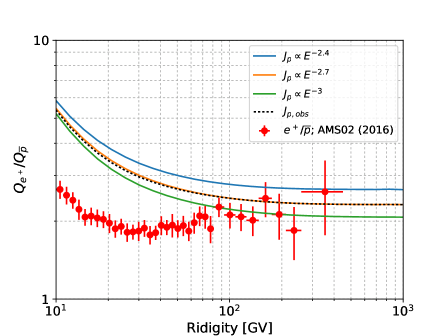
Figure 5: $e^{+}/\bar{p}$ flux ratio: AMS02 data compared to the secondary upper bound of Eq. (8). The upper bound ($e^{+}/\bar{p}$ source ratio) is shown with different assumptions for the proton spectrum in the secondary production regions. Systematic cross section uncertainties in $pp\to\bar{p},e^{+}$, not shown in the plot, are in the ballpark of 10%. Dashed black line shows the result evaluated for the locally measured $J_{p}$, while blue and green lines show the result for harder and softer proton flux, respectively, as specified in the legend. Taken from Blum et al. (2017b).

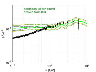
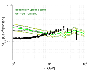
Figure 6: Left: $e^{+}/e^{\pm}$ flux ratio. AMS02 data compared to the secondary upper bound, evaluated directly from B/C data by using the equivalent form of Eq. (3) applied to $e^{+}$. Systematic uncertainties are represented as in Fig. 2. Right: same as on the left but showing the $e^{+}$ flux.

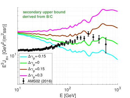
Figure 7: Same as the right panel of Fig. 6, but showing in cyan, green, red, and magenta the resulting secondary upper limit on $J_{e^{+}}$ that obtains if the high energy proton spectrum in the spallation region is changed w.r.t. the locally measured spectrum by a factor $\left(\mathcal{R}/200~{}{\rm GV}\right)^{\Delta\gamma_{p}}$, starting at $\mathcal{R}>200$ GV, with $\Delta\gamma_{p}=-0.15,\,0,\,0.15,\,0.3$, respectively.

Pause to appreciate this situation: The measured $e^{+}/\bar{p}$ ratio does not exceed and is always comparable to the secondary upper bound. Moreover, the $e^{+}/\bar{p}$ ratio saturates the bound over an extended range in rigidity. Taking into account that, as we saw in the previous section, $\bar{p}$ are likely secondary (certainly dominated by secondary production), it is natural to deduce that AMS02 is observing secondary $e^{+}$ as well, and propagation energy losses are small.

A compatible but less robust way to represent the secondary $e^{+}$ upper bound is directly from the B/C grammage, as we did for $\bar{p}$ in Fig. 2. Namely, we write

$$n_{e^{+}}(\mathcal{R}) \lesssim \frac{n_{\rm B}(\mathcal{R})}{Q_{\rm B}(\mathcal{R})}Q_{e^{+}}(\mathcal{R}).$$ (9)

The result is shown in Fig. 6. On the left panel the measured total $e^{\pm}$ flux of AMS02 Vagelli (2016) is used to define the $e^{+}/e^{\pm}$ ratio upper bound from Eq. (9). On the right panel we show the upper bound on the $e^{+}$ flux. We stress that Eq. (9) (and thus Fig. 6), similarly to the $\bar{p}/p$ situation exhibited in Fig. 3, is more sensitive to the unknown CR spectra in the spallation regions than is the $e^{+}/\bar{p}$ ratio of Fig. 5. In Fig. 7 we show how the bound is modified if one allows the proton spectrum in the secondary production sites to vary w.r.t. the locally measured proton flux. Models that realise this possibility include Cowsik and Burch (2009); Burch and Cowsik (2010); Cowsik et al. (2014); Blasi (2009); Blasi and Serpico (2009); Mertsch and Sarkar (2009); Ahlers et al. (2009); Kachelriess et al. (2011); Cholis et al. (2017); Kachelrie et al. (2015); Thomas et al. (2016), reviewed in Sec. III.5. The sensitivity of the bound in Fig. 7 to proton flux variation should be compared to the insensitivity of the more robust $e^{+}/\bar{p}$ ratio of Fig. 5.

For later convenience it is useful to define the loss suppression factor $f_{e^{+}}$ via

$$\frac{n_{e^{+}}}{n_{\bar{p}}} = f_{e^{+}}(\mathcal{R})\frac{Q_{e^{+}}(\mathcal{R})}{Q_{\bar{p}}(\mathcal{R})}.$$ (10)

In Fig. 8 we show $f_{e^{+}}$ as derived from Fig. 5. The upper bound for secondary $e^{+}$ is $f_{e^{+}}(\mathcal{R})\leq 1$. We find that $f_{e^{+}}(\mathcal{R})$ is never much smaller than unity, and approaches unity from below for increasing $\mathcal{R}$.

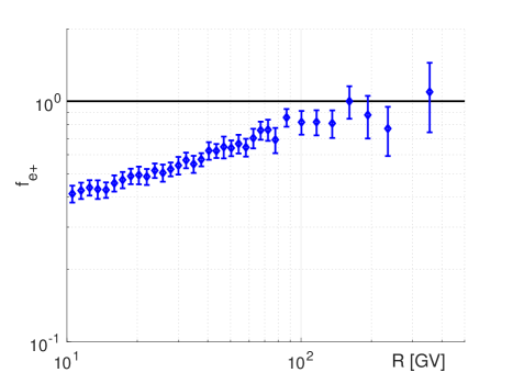
Figure 8: $f_{e^{+}}$ extracted from Fig. 5. The upper bound for secondary $e^{+}$ reads $f_{e^{+}}\leq 1$. Error bars reflect the measurement error on $\bar{p}/e^{+}$ reported in Aguilar et al. (2016a). Systematic cross section uncertainties in $pp\to\bar{p},e^{+}$, not shown in the plot, are in the ballpark of 10%.

In considering this behaviour it is important to note that theoretically the possible range of the suppression factor is $0<f_{e^{+}}<\infty$: this just says that a prominent primary source of $e^{\pm}$ – say, a nearby pulsar – could make the $e^{+}$ flux as large as we wish in comparison to the secondary upper bound; while strong radiative losses, if at work, could extinguish the flux.

We conclude that AMS02 results hint for a secondary origin for $e^{+}$ Blum et al. (2013). If $e^{+}$ are secondary, then Fig. 5 suggests that the effect of energy loss in suppressing the $e^{+}$ flux is never very important, and possibly becomes less significant as we go to higher $e^{+}$ energy. As we shall see, this behaviour contradicts the expectations within common models of CR propagation. To appreciate this point we must venture into somewhat more muddy waters of CR astrophysics and consider the interplay of $e^{+}$ energy losses with the effects of propagation.

III.2 Radiative energy loss vs. propagation time vs. grammage

The name of the game is to figure out the interplay of $e^{+}$ energy loss with CR propagation: this is needed either to establish the necessity of a primary $e^{+}$ source, or to understand the lessons for CR propagation if $e^{+}$ are secondary.

The $e^{+}$ radiative cooling time is

$$t_{\rm cool}(\mathcal{R}) = -\frac{\mathcal{R}}{\dot{\mathcal{R}}}\;\;.$$ (11)

At high energy $\mathcal{R}>10$ GV, energy loss is dominated by synchrotron and IC. In the Thomson regime Blumenthal and Gould (1970)

$$t_{\rm cool}(\mathcal{R}) = \frac{3m_{e}^{4}}{4\sigma_{T}U_{T}}\approx 30\left(\frac{\mathcal{R}}{10~{}{\rm GV}}\right)^{-1}\left(\frac{U_{T}}{1~{}{\rm eVcm^{-3}}}\right)^{-1}~{}{\rm Myr},$$ (12)

where $U_{T}$ is the sum of radiation and magnetic field energy densities. Thus, in the Thomson regime $t_{\rm cool}\propto\mathcal{R}^{-1}$. Bremstrahlung and Klein-Nishina corrections soften this behaviour to $t_{\rm cool}\sim\mathcal{R}^{-\gamma_{c}}$ with $\gamma_{c}<1$, as we discuss in Sec. III.4.

Consider the qualitative behaviour of $f_{e^{+}}$. We expect $f_{e^{+}}$ to increase monotonically as a function of $t_{\rm cool}/t_{\rm esc}$, where $t_{\rm esc}$ is the CR propagation time, defined in some convenient way to parametrise the typical time a CR spends in the system from the time of production until the time of detection at Earth.

In the limit $t_{\rm cool}/t_{\rm esc}\gg 1$, we expect $f_{e^{+}}\to 1$; this is because in this limit, a typical CR trajectory lasts much less time than the time it takes an $e^{+}$ to lose a significant amount of its initial energy. Thus in this limit relativistic $e^{+}$ and $\bar{p}$ at the same $\mathcal{R}$ propagate in the same way and the observed $e^{+}/\bar{p}$ ratio reflects the secondary production rate ratio $Q_{e^{+}}/Q_{\bar{p}}$. In the opposite limit, $t_{\rm cool}/t_{\rm esc}\ll 1$, we expect $f_{e^{+}}\ll 1$ because $e^{+}$ lose most of their energy on their way from production to detection, while the corresponding $\bar{p}$ propagate unaffected.

Given an estimate of $t_{\rm cool}$, Fig. 8 is therefore a measurement of the CR propagation time. The detailed interpretation of the form of $f_{e^{+}}$, however, is model-dependent. To demonstrate this point, in App. B we calculate $f_{e^{+}}$ for two propagation model examples: a version of the leaky-box model (LBM), and a one-dimensional thin disc+halo diffusion model.

We emphasize that both of these models satisfy Eq. (1). Therefore, calibrating the relevant free parameters in either model to reproduce $X_{\rm esc}\sim\mathcal{R}^{-0.4}$ according to Fig. 1 would make these models automatically reproduce Fig. 2, consistent with AMS02 $\bar{p}/p$ data. Fig. 9 shows $f_{e^{+}}$ as obtained for the two models, with propagation parameters calibrated consistently with B/C and $\bar{p}/p$. We take representative values of $\gamma_{i}=2$ and 2.7 for the primary proton spectral index. The numerical value of $f_{e^{+}}$ differs between the LBM and diffusion models, despite having calibrated both of these models to match B/C and $\bar{p}/p$.

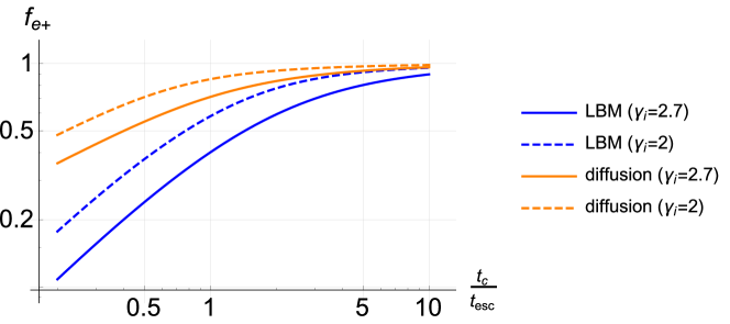
Figure 9: The $e^{+}$ flux loss suppression factor $f_{e^{+}}$, as function of the cooling to escape time ratio, for the LBM and diffusion models with different values of the primary proton spectral index $\gamma_{i}$ in the secondary production region. Details of the calculation are given in App. B.

While the diffusion model and the LBM differ in the form of $f_{e^{+}}$ they predict, both models share a common feature: in both of the models, the rigidity-dependent column density of ISM traversed by CRs is proportional to the rigidity-dependent propagation time, $X_{\rm esc}(\mathcal{R})\propto t_{\rm esc}(\mathcal{R})$.

This proportionality between $X_{\rm esc}$ and $t_{\rm esc}$ is more general than the specific models we looked at. It holds, for example, for commonly adopted diffusion models Strong et al. (2007) that assume a rigidity independent diffusion boundary. Because the grammage $X_{\rm esc}$ must be fit in phenomenologically consistent versions of these models to match B/C, sub-Fe/Fe, and $\bar{p}/p$ data, these models satisfy

$$t_{\rm esc}(\mathcal{R})\propto X_{\rm esc}(\mathcal{R})\propto\mathcal{R}^{-0.4},$$ (13)

where in the numerical assignment we adopt, for simplicity, the approximate fit of Ref. Blum et al. (2013).

Using Eq. (12) gives $t_{\rm cool}(\mathcal{R})\propto\mathcal{R}^{-\gamma_{c}}$ with $\gamma_{c}=1$, so propagation models that satisfy Eq. (13) predict that the ratio $t_{\rm cool}(\mathcal{R})/t_{\rm esc}(\mathcal{R})\propto\mathcal{R}^{0.4-\gamma_{c}}\sim\mathcal{R}^{-0.6}$ must decrease with increasing rigidity. As a result, because $f_{e^{+}}$ scales as a positive power of $t_{\rm cool}(\mathcal{R})/t_{\rm esc}(\mathcal{R})$, these models predict that the effect of losses should become increasingly more important at high energy: $f_{e^{+}}(\mathcal{R})$ should decrease at rising $\mathcal{R}$. This is the opposite trend to that inferred from data in Figs. 5-8.

To maintain the hypothesis of secondary $e^{+}$, the fact that the observed $f_{e^{+}}$ approaches unity with increasing rigidity implies that the propagation time $t_{\rm esc}$ cannot be much larger than the cooling time $t_{\rm cool}$, and is decreasing with rigidity faster than $t_{\rm cool}$. This means that $t_{\rm esc}$ decreases with rigidity faster than $X_{\rm esc}$, in contradiction to Eq. (13).

We are faced with two possibilities. Either take the coincidence of the observed $e^{+}/\bar{p}$ ratio with pp branching fractions (Figs. 5-8) as a hint that CR $e^{+}$ are secondary, in which case something basic is not right in the commonly adopted CR diffusion models: the CR grammage cannot be proportional to the CR propagation time. Or, accept the diffusion models and invoke a primary source for $e^{+}$, like dark matter annihilation or pulsars, in which case some primary source parameters would need to be tuned to reproduce the observed $e^{+}/\bar{p}$ ratio as an accident.

This is a good point to comment on statements in the literature, that advocated the presence of an $e^{+}$ primary source based on a rising $e^{+}/e^{\pm}$ fraction. Two representative examples are Adriani et al. (2009) and Serpico (2009). Ref. Adriani et al. (2009), and numerous following works, based the call for primary $e^{+}$ on the observation that a rising $e^{+}/e^{\pm}$ would be inconsistent with secondary $e^{+}$ as expected in a certain diffusion model Moskalenko and Strong (1998). However, phenomenological models such as Moskalenko and Strong (1998) are constructed with many simplifying assumptions, ranging from steady state and homogeneous diffusion to the geometry and boundary conditions of the CR halo Strong et al. (2007). Some of these assumptions may not apply to Nature. We explore alternative ideas with secondary $e^{+}$ in Sec. III.5.

Ref. Serpico (2009) argued that a rising $e^{+}/e^{\pm}$ requires primary $e^{+}$ because $e^{-}$ and $e^{+}$ suffer radiative energy losses in the same way, and because the primary $e^{-}$ source spectrum cannot be softer than that of the secondary $e^{+}$. The problem with this argument is that the injection spectrum of primary $e^{-}$ is unknown, and the propagation paths of $e^{+}$ and $e^{-}$ may differ because their production sites as secondaries vs. accelerated primaries, respectively, may be different. In this case, $e^{-}$ may suffer additional energy losses as compared to $e^{+}$. We will see model examples for this, too, in Sec. III.5.

Finally, it is important to note that the high energy $e^{+}$ data Adriani et al. (2009); Aguilar et al. (2013); Ting represent a new observational probe of CR propagation at high rigidity $\mathcal{R}>10$ GV: it tests the propagation models where they were not tested before. B/C data measures $X_{\rm esc}$; as we have seen, other stable secondary nuclei data such as $\bar{p}/p$ do not give much of a new test: they are essentially consistency checks of the hypothesis that different CR species sample similar $X_{\rm esc}$, a fact for which early evidence already existed Engelmann et al. (1990); Webber et al. (2003); Gaisser and Schaefer (1992). In contrast, the $e^{+}$ data is sensitive to the a-priori independent quantity $t_{\rm esc}$. The fact that $e^{+}$ could eventually provide such a test of the models was pointed out already in Ginzburg and Ptuskin (1976); Ginzburg et al. (1990), long before PAMELA and AMS02 made this test come to life.

Besides from $e^{+}$, no other CR data to date accesses $t_{\rm esc}$ in the same range in rigidity $\mathcal{R}\mathrel{\hbox to0.0pt{\lower 4.0pt\hbox{\hskip 1.0pt$\sim$}\hss}\raise 1.0pt\hbox{$>$}}100$ GV. What comes nearest are measurements of the effect of radioactive decay of secondary Be, Al, and Mg isotopes. In Sec. III.3 we consider these data as a model-independent test of the secondary $e^{+}$ hypothesis. As of today, the test is based on early measurements Webber and Soutoul (1998); Engelmann et al. (1990) and supports the idea of secondary $e^{+}$ Katz et al. (2010), but is inconclusive due to systematic uncertainties. A better test should become possible in the near future with AMS02 data, and we devote some time to explain the key physics.

III.3 A test with radioactive nuclei

Measurements of the suppression of the flux of secondary radioactive nuclei due to decay in flight constrain the CR propagation time $t_{\rm esc}$ Shapiro and Silberberg (1970); Webber and Soutoul (1998); Ptuskin (1999); Simpson, J. A. and Garcia-Munoz, M. (1988); Ptuskin and Soutoul (1998); Yanasak et al. (2001); Donato et al. (2002); Putze et al. (2010); Blum (2011); Shibata and Ito (2007). The idea is that a relativistic radioactive nucleus with rest frame lifetime $\tau_{d}$, mass number $A$ and charge $eZ$ has an observer frame lifetime

$$t_{d}(\mathcal{R}) \approx \sqrt{1+\frac{e^{2}Z^{2}\mathcal{R}^{2}}{A^{2}m_{p}^{2}}}\tau_{d},$$ (14)

when observed as CR. Given a secondary radioactive species like ¹⁰Be, we can compute the prediction for its density, discarding the effect of decay, and compare the result to the observed density. This allows to define a decay suppression factor that can be extracted directly from data:

$$f_{{}^{10}\rm Be}(\mathcal{R}) = \frac{n_{\rm{}^{10}Be}(\mathcal{R})}{n_{\rm{}^{10}Be,\,no\,decay}(\mathcal{R})}\approx\frac{n_{\rm{}^{10}Be}(\mathcal{R})}{\frac{Q^{+}_{\rm{}^{10}Be}(\mathcal{R})}{1+X_{\rm esc}(\mathcal{R})\frac{\sigma_{{}^{10}\rm Be}}{m}}}.$$ (15)

Here, the numerator is supposed to be taken directly from measurement, while the denominator is a theory output but is, again, data-driven based on fragmentation cross sections, B/C and primary CR spectra. In the last expression we used Eqs. (1) and (4), and noted that for stable secondary species $i$ Eq. (1) implies

$$n_{i}(\mathcal{R}) \approx \frac{Q^{+}_{i}(\mathcal{R})}{1+X_{\rm esc}(\mathcal{R})\frac{\sigma_{i}}{m}},$$ (16)

where $Q^{+}_{i}(\mathcal{R})$ is the positive production term in the net source $Q_{i}$. (As before, $\sigma_{i}/m$ is the total inelastic cross section of $i$ per ISM particle mass.)

We expect the qualitative behaviour of $f_{{}^{10}\rm Be}(\mathcal{R})$ to depend on the CR propagation time $t_{\rm esc}$ via the ratio $t_{d}(\mathcal{R})/t_{\rm esc}(\mathcal{R})$: for $t_{d}(\mathcal{R})/t_{\rm esc}(\mathcal{R})\to\infty$ we should have $f_{{}^{10}\rm Be}(\mathcal{R})\to 1$, while for $t_{d}(\mathcal{R})/t_{\rm esc}(\mathcal{R})\to 0$ we expect $f_{{}^{10}\rm Be}(\mathcal{R})\ll 1$. Because $t_{\rm esc}(\mathcal{R})$ decreases with increasing $\mathcal{R}$, and $t_{d}(\mathcal{R})$ (for relativistic nuclei) increases as $t_{d}\propto\mathcal{R}$, it is clear that $f_{{}^{10}\rm Be}(\mathcal{R})$ should approach unity with increasing $\mathcal{R}$. Since $t_{d}$ is known from laboratory data, a measurement of $f_{{}^{10}\rm Be}$ provides a constraint on $t_{\rm esc}$.

Experimental data on radioactive nuclei is divided in two categories: isotopic data such as ¹⁰Be/⁹Be, and elemental (or charge) data like Be/B in which the numerator denotes the sum of Be isotopes (^7,9,10Be) and the denominator the sum of B isotopes (^10,11B).

Isotopic ratios are experimentally challenging to measure at high energy. As a result, current data on ¹⁰Be/⁹Be is limited to low rigidity $\mathcal{R}\lesssim 1$ GV. This introduces significant theory uncertainty in the interpretation of these data as effects such as solar modulation, energy-dependence in the nuclear fragmentation cross sections, and various propagation effects that change CR energy during propagation become important (see e.g. Ptuskin et al. (1996)). Nevertheless, diffusion models have traditionally used this low energy data to calibrate the models Strong et al. (2007), extrapolating the result to the relativistic range. AMS02 is expected to improve the situation with the ability to measure ¹⁰Be/⁹Be up to $\mathcal{R}\sim 10$ GV.

Elemental ratios can be measured to high energy Webber and Soutoul (1998). The challenge here is that the contribution of the radioactive ¹⁰Be isotope to the total Be flux is never expected to exceed about $\sim 30\%$, based on our knowledge of partial fragmentation cross sections like ¹²C$\to^{10}$Be vs. ¹²C$\to^{7,9}$Be, etc. As a result, the Be/B ratio is limited to the range $0.3\lesssim{\rm Be/B}\lesssim 0.4$ or so, making the interpretation particularly sensitive to fragmentation cross section uncertainties. The situation with other relevant elemental ratios, Al/Mg and Cl/Ar, is similar.

The Be/B ratio derived from early measurements of Be and B fluxes by the HEAO3 mission is shown in Fig. 10 (blue markers) Webber and Soutoul (1998); Engelmann et al. (1990). Recently, AMS02 reported preliminary results for Be/B Ting extending to very high energy, shown in red. The saturation point $f_{{}^{10}\rm Be}\to 1$ is, for the first time, clearly manifest in this data as the observed Be/B saturates the no-decay secondary prediction.

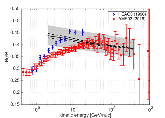
Figure 10: The elemental flux ratio Be/B. HEAO3 data shown in blue; preliminary data from AMS02 in red. The no-loss secondary prediction is shown by black line. Shaded band shows the effect of varying by $\pm 10$% the cumulative cross section for B production, $\sigma_{\rm CNO\to B}$. Dashed lines show the effect of varying the cross sections for ¹¹B$\to^{7,9,10}$Be, in a correlated way, by $\pm 20$%.

The definition of the decay suppression factor $f_{{}^{10}\rm Be}(\mathcal{R})$ is analogous to that of the loss suppression factor $f_{e^{+}}(\mathcal{R})$ defined in Eq. (10) for secondary $e^{+}$. However, radioactive decay is not quite the same as radiative energy loss: the former eliminates the CR altogether, while the latter just degrades it in energy. Moreover, the $\mathcal{R}$ dependence of $t_{d}(\mathcal{R})\sim\mathcal{R}$ for radionuclei is essentially opposite to $t_{\rm cool}(\mathcal{R})\sim\mathcal{R}^{-1}$ for $e^{+}$. Fig. 11 illustrates the behaviour of $t_{d}$ and $t_{\rm cool}$.

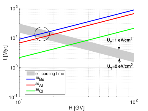
Figure 11: Radioactive decay vs. $e^{+}$ energy loss. An estimate of the $e^{+}$ cooling time $t_{\rm cool}$ is shown by grey band, obtained for $U_{T}$ between 1-2 eV/cm³, neglecting Klein-Nishina corrections. The observer frame lifetimes of CR ¹⁰Be, ²⁶Al, and ³⁶Cl are shown by blue, red, and green lines, respectively. Around $\mathcal{R}\sim 15$ GV (kinetic energy per nucleon $k\sim 5$ GeV/nuc), the observer frame lifetime of ¹⁰Be approximately coincides with the cooling time of CR $e^{+}$.

Ref. Katz et al. (2010) pointed out an approximate, but model independent way in which radiative energy losses and radioactive decay can be put on similar footing. Consider the contribution of radioactive decay in a general, local transport equation. Decay introduces a term to the continuity equation for radionucleus $i$,

$$\left(\frac{\partial n_{i}}{\partial_{t}}\right)_{\rm decay} = -\frac{n_{i}(\mathcal{R})}{t_{d,i}(\mathcal{R})}.$$ (17)

Energy loss for $e^{+}$, in comparison, is captured by:

$$\left(\frac{\partial n_{e^{+}}}{\partial_{t}}\right)_{\rm energy\,loss} = \frac{\partial}{\partial\mathcal{R}}\left(\dot{\mathcal{R}}n_{e^{+}}\right)=-\frac{n_{e^{+}}(\mathcal{R})}{\tilde{t}_{\rm cool}(\mathcal{R})},$$ (18)

where we define

$$\frac{1}{\tilde{t}_{\rm cool}(\mathcal{R})} = -\left[\frac{\partial\log\left(\frac{\mathcal{R}n_{e^{+}}}{t_{\rm cool}}\right)}{\partial\log\mathcal{R}}\right]\frac{1}{t_{\rm cool}(\mathcal{R})}.$$ (19)

The observed $e^{+}$ flux in the range $\mathcal{R}\sim(10-500)$ GV is roughly a power law $n_{e^{+}}\sim\mathcal{R}^{-\gamma_{e^{+}}}$ with $\gamma_{e^{+}}$ in the range $(2.75-3)$. For $t_{\rm cool}$ not far from the Thomson regime, $t_{\rm cool}\sim\mathcal{R}^{-1}$, the logarithmic term in Eq. (19) is therefore a weak function of $\mathcal{R}$, varying in the range $-\left[\frac{\partial\log\left(\mathcal{R}^{2}n_{e^{+}}\right)}{\partial\log\mathcal{R}}\right]\sim(0.75-1)$. We learn that, due to the steeply falling $e^{+}$ flux, decay and energy loss are represented by a similar form in the continuity equation.

A model independent check of the hypothesis of secondary $e^{+}$ is therefore obtained by comparing the observed $f_{e^{+}}(\mathcal{R}^{*})$ for $e^{+}$, and $f_{i}(\mathcal{R}^{*})$ for radionucleus $i$, at the particular rigidity $\mathcal{R}=\mathcal{R}^{*}$ in which $t_{d,i}(\mathcal{R}^{*})=t_{\rm cool}(\mathcal{R}^{*})$. Referring to Fig. 11, we see that for ¹⁰Be, with a reasonable estimate of $U_{T}$, $\mathcal{R}^{*}\sim 15$ GV. This is illustrated by a circle in the plot. For this rigidity, Fig. 8 suggests

$$f_{e^{+}}(15~{}{\rm GV}) \sim 0.4-0.5.$$ (20)

From the HEAO3 data Engelmann et al. (1990) analysis of Webber and Soutoul (1998), Ref. Katz et al. (2010) found

$$f_{{}^{10}\rm Be}(15~{}{\rm GV}) \sim 0.3-0.4.$$ (21)

Consistent results obtain for the Al/Mg and Cl/Ar data.

Significant systematic uncertainty affects this analysis, manifest in Fig. 10 by the cross section uncertainty as well as the mismatch between HEAO3 and AMS02 preliminary results. Nevertheless, we can conclude that this test of radionuclei data is consistent with secondary $e^{+}$. Upcoming results from AMS02 Ting should allow to improve this test.

Finally, Ref. Blum (2011) suggested that the rigidity dependence of $t_{\rm esc}$ can be constrained by comparing the decay suppression factor $f_{i}$ for different species of radionuclei measured at the same observer frame lifetime and thus – because different nuclei have different rest frame lifetimes – at different rigidities.

Fig. 12 illustrates this point with HEAO3 data Engelmann et al. (1990); Webber and Soutoul (1998). While, again, systematic and statistical uncertainties in this data are large, the idea is promising: a rapidly decreasing $t_{\rm esc}(\mathcal{R})$, as needed to reconcile secondary $e^{+}$ with a rising $f_{e^{+}}(\mathcal{R})$, would manifest in the radionuclei data by resolving the combined radionuclei data set into three different $f_{i}$ curves for Be/B (controlled by $\tau_{{}^{10}\rm Be}=2.2$ Myr), Al/Mg ($\tau_{{}^{26}\rm Al}=1.3$ Myr), and Cl/Ar ($\tau_{{}^{36}\rm Cl}=0.44$ Myr).

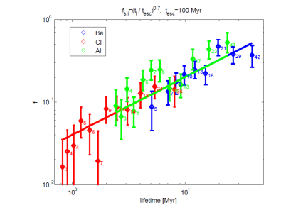
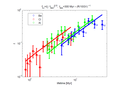
Figure 12: Radioactive nuclei data from HEAO3 Engelmann et al. (1990); Webber and Soutoul (1998), presented in terms of the decay suppression factor $f_{i}$ vs observer frame lifetime derived from Eq. (14). Numbers next to each point denote the rigidity $\mathcal{R}$ (in GV) for that nucleus species at that observer frame lifetime. Left: fit assuming $\mathcal{R}$-independent $t_{\rm esc}$. If this turns out to be the correct fit, then CR $e^{+}$ are not secondary. Right: fit assuming $t_{\rm esc}\propto\mathcal{R}^{-1}$, roughly as needed to obtain $f_{e^{+}}$ that is rising or flat with $\mathcal{R}$. Current uncertainties do not allow a clear preference, but upcoming AMS02 data, with some improvement in fragmentation cross section analyses (see e.g. Tomassetti (2015)), can change the picture. From Ref. Blum (2011).

III.4 Implications of secondary $e^{+}$ for CR propagation

In this section we assume that $e^{+}$ are secondary, and review constraints on CR propagation that can be deduced in this case. Fig. 8 suggests that

$$f_{e^{+}}(\mathcal{R}=300~{}{\rm GV})\mathrel{\hbox to0.0pt{\lower 4.0pt\hbox{\hskip 1.0pt$\sim$}\hss}\raise 1.0pt\hbox{$>$}}0.7,$$ (22)

$$f_{e^{+}}(\mathcal{R}=10~{}{\rm GV})\mathrel{\hbox to0.0pt{\lower 4.0pt\hbox{\hskip 1.0pt$\sim$}\hss}\raise 1.0pt\hbox{$<$}}0.5.$$ (23)

Considering the two models depicted in Fig. 9 as representative examples, Eq. (22) implies $t_{\rm cool}(\mathcal{R}=300~{}{\rm GV})/t_{\rm esc}(\mathcal{R}=300~{}{\rm GV})\mathrel{\hbox to0.0pt{\lower 4.0pt\hbox{\hskip 1.0pt$\sim$}\hss}\raise 1.0pt\hbox{$>$}}1$ for the diffusion model, and $t_{\rm cool}(\mathcal{R}=300~{}{\rm GV})/t_{\rm esc}(\mathcal{R}=300~{}{\rm GV})\mathrel{\hbox to0.0pt{\lower 4.0pt\hbox{\hskip 1.0pt$\sim$}\hss}\raise 1.0pt\hbox{$>$}}3$ for the LBM. Eq. (23) implies $t_{\rm cool}(\mathcal{R}=10~{}{\rm GV})/t_{\rm esc}(\mathcal{R}=10~{}{\rm GV})\mathrel{\hbox to0.0pt{\lower 4.0pt\hbox{\hskip 1.0pt$\sim$}\hss}\raise 1.0pt\hbox{$<$}}0.4$ for the diffusion model, and $t_{\rm cool}(\mathcal{R}=10~{}{\rm GV})/t_{\rm esc}(\mathcal{R}=10~{}{\rm GV})\mathrel{\hbox to0.0pt{\lower 4.0pt\hbox{\hskip 1.0pt$\sim$}\hss}\raise 1.0pt\hbox{$<$}}1.5$ for the LBM.

Ignoring Klein-Nishina corrections (but see discussion below), we summarise these results by the constraints Blum et al. (2013),

$$t_{\rm esc}\left(\mathcal{R}=300~{}{\rm GV}\right) \leq t_{\rm cool}\left(\mathcal{R}=300~{}{\rm GeV}\right)$$ (24)

$$\sim 1{\rm~{}Myr}\left(\frac{\bar{U}_{T}}{{\rm 1~{}eVcm^{-3}}}\right)^{-1},$$

$$t_{\rm esc}\left(\mathcal{R}=10~{}{\rm GV}\right) > t_{\rm cool}\left(\mathcal{R}=10~{}{\rm GeV}\right)$$ (25)

$$\sim 30{\rm~{}Myr}\left(\frac{\bar{U}_{T}}{{\rm 1~{}eVcm^{-3}}}\right)^{-1}.$$

The RHS of Eqs. (24-25) is based on a rough estimate of the $e^{\pm}$ cooling time at the relevant energies, and as such is subject to O(1) uncertainty. Here $\bar{U}_{T}$ is the time-averaged total electromagnetic energy density (propagation path- and time-average of $U_{T}$ from Eq. (12)) in the propagation region. It is natural to expect that $\bar{U}_{T}$ depends on CR rigidity, both because the radiation and magnetic fields in the ISM are not uniformly distributed and because the Thomson limit for describing the losses is not exact.

One irreducible source for energy dependence in the effective value of $\bar{U}_{T}$ comes from Klein-Nishina corrections, that are neglected in Eqs. (24) and (25). The Thomson limit is not a good approximation for 20-300 GV positrons if $U_{T}$ contains a significant UV component, as may be the case judging from estimates of the Milky Way radiation field Hauser and Dwek (2001); Porter and Strong (2005); Crutcher et al. (2010). In terms of Eqs. (24-25), a plausible $\sim$50% UV contribution to $U_{T}$ implies that the effective value of $\bar{U}_{T}$ decreases between 10 GV to 300 GV by a factor of $\sim$2. More extreme possibilities were entertained in Stawarz et al. (2010).

Another feature that is not included in Eqs. (12,24-25) is bremsstrahlung losses. The bremsstrahlung radiation length is $\zeta\approx 60$ g/cm² Longair (1992), approximately independent of energy and insensitive to the H:He ratio in the ISM, such that the corresponding cooling time is $t_{\rm brem}\approx\zeta/(c\rho_{ISM})$. The energy loss term in the $e^{+}$ continuity equation takes a form similar to that of a fragmentation loss term for nuclei,

$$\frac{\partial}{\partial\mathcal{R}}\left(\dot{\mathcal{R}}n_{e}^{+}\right)_{\rm brem} \approx -\Gamma_{\rm brem}\,n_{e}^{+},$$ (26)

where

$$\Gamma_{\rm brem} = -\frac{c\rho_{ISM}}{\zeta}\left[\frac{\partial\log\left(\mathcal{R}n_{e}^{+}\right)}{\partial\log\mathcal{R}}\right].$$ (27)

For $n_{e^{+}}\sim\mathcal{R}^{-\gamma_{e^{+}}}$ with $\gamma_{e^{+}}\sim 2.75-3$, we have $\Gamma_{\rm brem}\approx C(c\rho_{ISM}/\zeta)$ with $C\sim 1.75-2$.

Using the similarity to fragmentation losses of nuclei, the $e^{+}$ loss suppression factor due to brem is

$$f_{e^{+},\rm brem} \approx \frac{1}{1+X_{\rm esc}\,\Gamma_{\rm brem}}.$$ (28)

In Fig. 13 we repeat the calculation of $f_{e}^{+}$, modding out (in green) the brem contribution using Eqs. (27-28) with $C=2$. Bremsstrahlung modifies $f_{e}^{+}$ by $\sim 40\%$ at $\mathcal{R}=10$ GV but becomes negligible at $\mathcal{R}\sim 100$ GV.

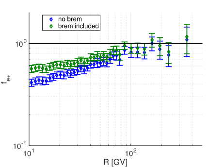
Figure 13: $f_{e^{+}}$ extracted from Fig. 5. Green markers: bremsstrahlung losses estimated from $X_{\rm esc}$ and subtracted from $f_{e^{+}}$. Blue markers same as in Fig. 8.

We can also estimate the average ISM density traversed by CRs. Using Eq. (46) together with Eqs. (24) and (25), we find

$$\bar{n}_{ISM}\left(\mathcal{R}=300\,{\rm GV}\right) \gtrsim 1\,\left(\frac{\bar{U}_{T}}{{\rm 1~{}eVcm^{-3}}}\right)\,{\rm cm^{-3}},\;\;\;$$ (29)

$$\bar{n}_{ISM}\left(\mathcal{R}=10\,{\rm GV}\right) \lesssim 0.15\,\left(\frac{\bar{U}_{T}}{{\rm 1~{}eVcm^{-3}}}\right)\,{\rm cm^{-3}},\;\;\;$$ (30)

assuming an ISM composition of 90%H+10%He by number.

Eqs. (29) and (30) suggest that the confinement volume of CRs may be decreasing with increasing CR rigidity, to the extent that CRs at $\mathcal{R}\sim 300$ GV spend much of their propagation time within the thin Galactic HI disc, with a scale height $h\simeq 200\,{\rm pc}$, while CRs at $\mathcal{R}\sim 10$ GV probe a larger halo Katz et al. (2010). There are other possibilities, however. For example, if a significant fraction of the grammage $X_{\rm esc}$ is accumulated during a short time in relatively dense regions, e.g. near the CR source, then the halo could be larger. Significant energy dependence in $\bar{U}_{T}$ could further affect the interpretation. For example, $\bar{U}_{T}\propto\mathcal{R}^{-0.6}$, inspired by $X_{\rm esc}\sim\mathcal{R}^{-0.4}$, would allow for a rigidity independent $\bar{n}_{ISM}$.

Finally, it is also possible that the CR distribution is not in steady state. In this case, the PAMELA and AMS02 $e^{+}$ may be teaching us about, e.g., a recent nearby burst of star formation and supernova explosions. Key guidelines for such models, that can be derived from Figs. 2 and 5, are that:

1. B, $\bar{p}$, and $e^{+}$ appear to be secondaries from the same spallation episode, and

2. the bulk of the spallation must not have occurred more than a few Myr in the past.

In the next section we review some ideas along these lines.

III.5 Models for secondary $e^{+}$ and $\bar{p}$

In this section we briefly review CR propagation models Katz et al. (2010); Cowsik and Burch (2009); Burch and Cowsik (2010); Cowsik et al. (2014); Blasi (2009); Blasi and Serpico (2009); Mertsch and Sarkar (2009); Ahlers et al. (2009); Kachelriess et al. (2011); Cholis et al. (2017); Shaviv et al. (2009); Kachelrie et al. (2015); Thomas et al. (2016) where $e^{+}$ come from secondary production.

In the nested leaky box model of Cowsik and Burch (2009); Burch and Cowsik (2010); Cowsik et al. (2014), the secondary reacceleration model of Blasi (2009); Blasi and Serpico (2009); Mertsch and Sarkar (2009); Ahlers et al. (2009); Kachelriess et al. (2011); Cholis et al. (2017), and the recent supernova model of Kachelrie et al. (2015); Thomas et al. (2016), a common theme is that the spectrum of primary CRs in the secondary production sites is different than the locally measured spectrum. As a result, the application of Eq. (1) for relating the B/C garmmage $X_{\rm esc}$ to secondary $\bar{p}$ and $e^{+}$ becomes inaccurate (see the discussion around and below Eq. (6)). This means that the success of Eq. (3), seen in Fig. 2 to reproduce the $\bar{p}/p$ ratio at $\mathcal{R}\lesssim 100$ GV based on locally measured proton and nuclei spectra, should be somewhat accidental in these models. At $\mathcal{R}\gtrsim 100$ GV, Fig. 2 is consistent with the possibility of a contribution to the spallation from a harder proton spectrum, although the systematic cross section and primary flux uncertainties prevent a sharp conclusion.

We emphasize that the asymptotic $e^{+}/\bar{p}$ ratio (that is the ratio when $e^{+}$ losses are not important) is insensitive to primary spectrum details, as can be seen in Fig. 5.

The spiral arm model of Shaviv et al. (2009) is an example to a set-up in which $e^{-}$ and $e^{+}$ come from different regions in the Galaxy and thus their propagation energy losses are different.

Ref. Katz et al. (2010) pointed out that a rigidity-dependent CR propagation volume could break the proportionality between $t_{\rm esc}$ and $X_{\rm esc}$, in accordance with the discussion of Sec. III.2. Considering the diffusion model of Sec. III.2 (with more details in App. B), for example, the idea is to let the boundary condition vary as $L=L(\mathcal{R})$. Using Eqs. (49) and (48) with $K\sim\mathcal{R}^{\delta},\,L\sim\mathcal{R}^{-\delta_{L}}$, we have $t_{\rm esc}^{\rm diff}(\mathcal{R})\sim X_{\rm esc}^{\rm diff}(\mathcal{R})\times\mathcal{R}^{-\delta_{L}}$. Fixing $X_{\rm esc}\sim\mathcal{R}^{-0.4}$ to comply with B/C and $\bar{p}/p$ data, setting $\delta_{L}\sim 0.4,\,\delta\sim 0$ the model can accommodate an $e^{+}$ loss suppression factor $f_{e^{+}}$ that is flat as function of $\mathcal{R}$ for $t_{\rm cool}\sim\mathcal{R}^{-0.8}$ (implying some rigidity dependence of $\bar{U}_{T}$ due to, e.g., Klein-Nishina effects and bremsstrahlung; see Sec. III.4). In the diffusion model, rigidity-dependent $L$ corresponds to non-separable rigidity and spatial dependence of the diffusion coefficient (the free escape boundary $L$ in these models mimics a region where the diffusivity diverges, $K\to\infty$). Considering the picture of resonant pitch-angle scattering of CR on magnetic field irregularities Blandford and Eichler (1987), non-separable rigidity and spatial dependence of $K$ means that the spectrum of magnetic field turbulence varies in the propagation region. $L$ decreasing with increasing $\mathcal{R}$ would occur if large scale turbulence decays faster than small scale turbulence at increasing distance from the Galactic disc. A rigidity-dependent confinement volume could also be realised in other settings Blum (2011). More quantitative analysis is required to test the idea further.

Further discussion of Cowsik and Burch (2009); Burch and Cowsik (2010); Cowsik et al. (2014); Shaviv et al. (2009); Blasi (2009); Blasi and Serpico (2009); Mertsch and Sarkar (2009); Ahlers et al. (2009); Kachelriess et al. (2011); Cholis et al. (2017) and of the idea of a rigidity-dependent CR confinement volume can be found in Katz et al. (2010). In the rest of this section we highlight the more recent model of Kachelrie et al. (2015); Thomas et al. (2016).

Ref. Kachelrie et al. (2015); Thomas et al. (2016) suggested that a supernova (SN) explosion occurring about 2 Myr ago at a distance of $\sim$100 pc from the solar system and injecting of the order of $10^{50}$ erg in CR protons could affect the spectra of primary and secondary CRs. The rate of SNe in the Milky Way is in the ballpark of 3 per century Adams et al. (2013). Divided by the gas disc area $A_{\rm dsc}\sim 10^{3}$ kpc², this gives $\sim 3$ SNe per (300 pc)² per Myr, consistent with the set-up in Kachelrie et al. (2015). The detection of CR ⁶⁰Fe Fry et al. (2016); Binns et al. (2016) is also consistent with a recent nearby SN.

Because $\bar{p}$ and $e^{+}$ in Kachelrie et al. (2015) are produced as secondaries and their propagation time – given roughly by the time since the SN – is of order a Myr such that $e^{+}$ energy losses are not important below a few hundred GeV, the coincidence of the $e^{+}/\bar{p}$ flux ratio with the secondary production rate ratio $Q_{e^{+}}/Q_{\bar{p}}$ could be naturally addressed, as long as the recent SN contribution dominates for both species.

The SN-originated proton flux in Kachelrie et al. (2015) dominates the local proton flux by a factor of $\gtrsim 3$ at $\mathcal{R}\lesssim 1$ TV, with the remaining flux assumed to come from an long time average of CR production in multiple earlier CR injection events. At the same time, the column density associated to the SN protons is $X\sim 0.3$ g/cm², about 30% of $X_{\rm esc}$ derived from local B/C at $\mathcal{R}=1$ TV (see Fig. 1). As a result of this tuning (large SN proton flux with small associated grammage, vs. small average proton flux with large grammage), the SN-related contribution to the $\bar{p}$ flux is about $\sim 50$% of the total at $\mathcal{R}\sim 100$ GV.

In the model of Ref. Kachelrie et al. (2015), the CR distribution exhibits large deviations from steady-state with local sources producing order of magnitude deviations on sub-kpc and sub-Myr distance and time scales, as compared to the large volume or long time average. This picture can be tested with gamma ray data, by studying the gamma ray emissivity of individual molecular clouds and comparing to average diffuse emission data. Studies along these lines are ongoing Ackermann et al. (2012b); Dermer et al. (2013); Strong (2015); Mizuno et al. (2016); Neronov et al. (2017).

III.6 On dark matter and pulsar models for primary $e^{+}$ or $\bar{p}$

Many studies in the literature ascribed the CR $e^{+}$ or $\bar{p}$ flux to a primary source, the most common examples being pulsars (see, e.g. Profumo (2011); Hooper et al. (2009); Malyshev et al. (2009); Blasi and Amato (2011); Di Mauro et al. (2014); Lee et al. (2011) and references to and therein) and dark matter annihilation (see, e.g. Gaskins (2016); Meade et al. (2010); Cholis and Hooper (2013); Hooper and Tait (2009) and references to and therein). In these works the primary source is assigned free parameters to describe the $e^{+}$ or $\bar{p}$ spectrum and injection rate into the ISM. Then, using some CR diffusion model to simulate propagation effects, the model parameters are adjusted to fit the observed antimatter flux.

While we do not think that current $\bar{p}$ or $e^{+}$ data motivate the introduction of primary sources beyond the secondary flux, the possibility of dark matter or pulsar contributions is nevertheless interesting enough to merit some consideration.

The cosmological evidence for dark matter (DM) is compelling, and it is natural to imagine that DM is also responsible for the flattening of galactic rotation curves and other astrophysical gravitational anomalies. If DM is composed of massive particles, then pair annihilation of these particles in the Galactic halo could indeed produce high energy CR antimatter (examples predating the PAMELA data include, e.g. Bottino et al. (1998); Feng et al. (2001); Donato et al. (2004)). It is interesting to compare the CR antimatter source characterising a simple, generic DM model, to the irreducible secondary background. Focusing on $\bar{p}$ for concreteness, the injection rate density from DM particle-anti-particle pair annihilation can be written as

$$q_{\bar{p},\rm DM} = \frac{n_{\chi}^{2}(\vec{r})\,\overline{\sigma v}}{4}\,\frac{dN_{\bar{p}}}{dE}$$

$$\approx 7\times 10^{-34}\left(\frac{m_{\chi}}{100~{}\rm GeV}\right)^{-3}\frac{dN_{\bar{p}}}{dx}\left(\frac{\overline{\sigma v}}{3\times 10^{-26}~{}\rm cm^{3}/s}\right)\left(\frac{\rho_{\chi}(\vec{r})}{0.3~{}\rm GeV/cm^{3}}\right)^{2}~{}{\rm cm^{-3}s^{-1}GeV^{-1}}.$$

Here $n_{\chi}$ and $\rho_{\chi}=m_{\chi}n_{\chi}$ are the DM number and mass densities (see e.g. Bahcall and Soneira (1984); Navarro et al. (1996); Merritt et al. (2005); Sellwood (2009); Romano-Diaz et al. (2008); Bovy and Tremaine (2012)) related by the DM mass $m_{\chi}$, $\overline{\sigma v}$ is the velocity-weighted mean annihilation cross section Jungman et al. (1996), and $dN_{\bar{p}}/dx$ with $x=E/m_{\chi}$ is the (dimensionless) differential energy spectrum of $\bar{p}$ produced per annihilation event.

The dimensionless spectrum $dN_{\bar{p}}/dx$ is typically suppressed close to the kinematical endpoint at $x=1$, i.e. $dN_{\bar{p}}/dx(x\approx 1)\ll 1$. To illustrate this we plot, in the left panel of Fig. 14, $dN_{\bar{p}}/dx$ as obtained for three sample annihilation channels: $\chi\bar{\chi}\to W^{+}_{L}W^{-}_{L}$ (blue), $\chi\bar{\chi}\to hh$ (orange), $\chi\bar{\chi}\to b\bar{b}$ (green). Solid (dashed) lines show the result for $m_{\chi}=1$ TeV ($m_{\chi}=200$ GeV).

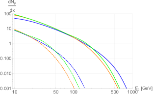
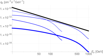
Figure 14: Left: Dimensionless spectra $dN_{\bar{p}}/dx$ for $\bar{p}$ produced in DM annihilation, calculated for $\chi\bar{\chi}\to W^{+}_{L}W^{-}_{L}$ (blue), $\chi\bar{\chi}\to hh$ (orange), $\chi\bar{\chi}\to b\bar{b}$ (green). Solid (dashed) lines show the result for $m_{\chi}=1$ TeV ($m_{\chi}=200$ GeV). Right: Comparison of the secondary source rate density (black) computed with the approximate Eq. (III.6), to DM annihilation source rate density. The DM annihilation spectra are for the $\chi\bar{\chi}\to W_{L}^{+}W_{L}^{-}$ channel and for DM mass of 1 TeV (solid) and 200 GeV (dashed). The thick, lower, DM lines show the result of Eq. (III.6), corresponding to a generic thermal relic DM model. The thin DM lines correspond to a multiplication of the output of Eq. (III.6) by a factor of 1000 for the 1 TeV case and 100 for the 200 GeV case.

The DM injection rate density can be compared to the secondary injection rate density,

$$q_{\bar{p},\rm sec} = \rho_{ISM}c\,Q_{\bar{p}}$$

$$\approx 4\times 10^{-33}\left(\frac{E}{100~{}\rm GeV}\right)^{-2.7}~{}{\rm cm^{-3}s^{-1}GeV^{-1}},$$

where $Q_{\bar{p}}$ is taken from Eqs. (2) and (6) and $\rho_{ISM}\approx 2\times 10^{-24}$ g/cm³ is a typical ISM mass density in the Galactic gas disc.

In the right panel of Fig. 14 we compare the DM injection rate density and the secondary injection rate density, taking the $\chi\bar{\chi}\to W_{L}^{+}W_{L}^{-}$ channel to represent the DM scenario. The thick, lower, DM lines show the result of Eq. (III.6), corresponding to a generic thermal relic DM model. The thin DM lines correspond to a multiplication of the output of Eq. (III.6) by a factor of 1000 for the 1 TeV case and 100 for the 200 GeV case. The irreducible secondary source is shown in black.

We conclude that a generic, thermal relic weakly interacting DM model predicts an $\bar{p}$ production rate density that is 2-3 orders of magnitude below the irreducible astrophysical secondary source as it occurs in a typical region in the Galactic gas disc. The picture for $e^{+}$ from DM annihilation is similar. On top of the source estimate, the CR flux resulting from the DM source enjoys a model-dependent enhancement factor compared with the secondary flux, if the DM halo extends over a large volume above and below the thin Galactic gas disc where the secondary spallation occurs. This enhancement factor could range from a factor of few to a factor of $\sim$100, given roughly by the ratio of the CR propagation volume to the volume of the gas disc, with some dependence on the unknown details of the DM density profile (see App. B in Ref. Agashe et al. (2010)). Even with this model-dependent volume enhancement factor, some enhancement mechanisms are often required to boost the DM annihilation cross section in a typical thermal relic DM model such that it could compete with the secondary background for CR energy above a few tens of GeV; examples include, e.g. Bovy (2009); Kuhlen and Malyshev (2009); Robertson and Zentner (2009). The required large DM annihilation cross sections are constrained by cosmological data Feng et al. (2010); Madhavacheril et al. (2014); Chan (2015); Ade et al. (2016), so that model building gymnastics is required to attribute observable high energy $e^{+}$ or $\bar{p}$ flux to DM.

Finally, consider the idea of pulsars as the source of $e^{+}$. Pulsars prevail the Galaxy Abdo et al. (2013); are likely producers of $e^{\pm}$ pairs Goldreich and Julian (1969); Gruzinov (2014); Philippov and Spitkovsky (2017); and have been suggested as possibly detectable sources of CR $e^{+}$ before the PAMELA era Atoyan et al. (1995); Boulares (1989). Thus, invoking pulsars as the origin of CR $e^{+}$ is sometimes considered an Occum’s Razor choice Profumo (2011).

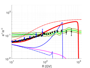
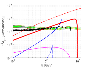
Figure 15: Concerning a pulsar interpretation for CR $e^{+}$. Left: $e^{+}/e^{\pm}$, Right: $e^{+}$ flux. In both panels, the thick red line shows the output for a pulsar model that was fit in Malyshev et al. (2009) to match the then available PAMELA $e^{+}/e^{\pm}$ (blue markers on left) Adriani et al. (2009) and ATIC, HESS and FERMI $e^{\pm}$ Chang et al. (2008); Aharonian et al. (2008, 2009); Abdo et al. (2009) data. Additional lines show the output of the same model when free parameters are varied within part of the range deemed viable in Malyshev et al. (2009); see text for details. The secondary $e^{+}$ upper limit derived from B/C data with no free parameters is shown in green.

However, the production rate of $e^{+}$ by pulsars and the spectrum of the $e^{\pm}$ flux when it is finally released into the ISM are unknown. Therefore, pulsar models for CR $e^{+}$ take both the $e^{+}$ injection rate and spectrum as free, or at least poorly constrained parameters of the model, and fit these parameters to the $e^{+}$ data along with a set of propagation model parameters and along with additional free parameters to describe, as needed, the remaining primary $e^{-}$ flux on top of the pulsar contribution. With this phenomenological freedom in fitting the flux, the coincidence with the secondary upper limit seen in Figs. 5-6 is a surprise: a fine-tuned accident from the point of view of these models.

In Fig. 15 we demonstrate this point by comparing the prediction of a pulsar model from Ref. Malyshev et al. (2009) to recent AMS02 $e^{+}$ data. In both panels, the thick red line shows the output for a pulsar model that was fit in Malyshev et al. (2009) to match the then available PAMELA $e^{+}/e^{\pm}$ Adriani et al. (2009) and ATIC, HESS and FERMI $e^{\pm}$ Chang et al. (2008); Aharonian et al. (2008, 2009); Abdo et al. (2009) data; see Fig. 2 in Malyshev et al. (2009). To see what happens to this model when some (a-priori unknown) parameters are varied, we show in red dashed: the result if the assumed age of the pulsar is reduced by a factor of 3; magenta: assumed injection spectral index $n=1.99$ (vs. $n=1.6$ in Ref. Malyshev et al. (2009)’s fit), $e^{\pm}$ injection power reduced by factor of 3, and cut-off energy reduced by factor 20; blue smooth: $n=1$, injection power up by factor 5, age up by factor 3; blue dashed: $n=1$, injection power down by factor 5, age up by factor 6.

IV Composite anti-nuclei: $\rm\bar{d}$ and $\overline{\rm{}^{3}He}$

Composite CR anti-deuterium ($\rm\bar{d}$) and anti-helium ($\overline{\rm{}^{3}He}$) have long been suggested as probes of dark matter Donato et al. (2000); Baer and Profumo (2005); Donato et al. (2008); Brauninger and Cirelli (2009); Kadastik et al. (2010); Cui et al. (2010); Dal and Kachelriess (2012); Ibarra and Wild (2013a); Fornengo et al. (2013); Carlson et al. (2014); Aramaki et al. (2016b), as their secondary astrophysical production was thought to be negligible Chardonnet et al. (1997); Duperray et al. (2005); Ibarra and Wild (2013b); Cirelli et al. (2014); Herms et al. (2017). These references, and references to and within them, cover extensively the exciting possibility that dark matter annihilation or even primordial black hole evaporation could in principle produce a detectable flux of $\rm\bar{d}$ and/or $\overline{\rm{}^{3}He}$ in current and upcoming experiments such as GAPS Aramaki et al. (2016a), BESS Abe et al. (2012, 2012), and AMS02 Giovacchini and Choutko (2007); Kounine . Therefore, in the current review we do not enter further discussion of hypothetical exotic sources.

However, exotic sources aside, how does one actually predict the irreducible secondary flux?

Using our tools from Sec. II, CR propagation is not a serious difficulty when it comes to stable, relativistic, secondary nuclei – and antinuclei, like $\bar{p}$, $\rm\bar{d}$ and $\overline{\rm{}^{3}He}$. The challenge for CR $\rm\bar{d}$ and $\overline{\rm{}^{3}He}$ is set instead by inadequate particle physics data. Astrophysical anti-nuclei are dominantly produced in pp collisions, for which relevant cross section data is scarce when it exists at all. This has led attempts to calculate the flux of $\rm\bar{d}$ and $\overline{\rm{}^{3}He}$ into various extrapolations, resulting with large and difficult to quantify systematic uncertainty.

A compilation of predictions of the secondary $\rm\bar{d}$ and $\overline{\rm{}^{3}He}$ fluxes from the literature is shown in Fig. 16 (left and right panels, respectively). To date no detection of either $\rm\bar{d}$ or $\overline{\rm{}^{3}He}$ was officially announced by any experiment, although news of possible detection were reported by AMS02 in 2016.

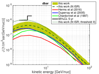
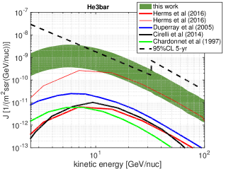
Figure 16: Left: estimates of the secondary CR $\rm\bar{d}$ flux. Right: estimates of the secondary CR $\overline{\rm{}^{3}He}$ flux. Shaded bands denote the predictions of Blum et al. (2017a), based on HBT data. AMS02 $\rm\bar{d}$ flux sensitivity (5-yr, 95%CL) in the kinetic energy range 2.5-4.7 GeV/nuc, as estimated in Aramaki et al. (2016b), is shown in solid line. AMS02 $\overline{\rm{}^{3}He}$ flux sensitivity (5-yr, 95%CL), derived from the $\overline{\rm{}^{3}He}/$He estimate of Kounine , is shown in dashed line. For more details, see Blum et al. (2017a).

A recent attempt at tackling the cross section problem in $pp\to\rm\bar{d},\,\overline{\rm{}^{3}He}$ production was done in Blum et al. (2017a), which used a new technique burrowed from heavy ion femtoscopy Lisa et al. (2005); Scheibl and Heinz (1999). The $\overline{\rm{}^{3}He}$ flux predicted in Blum et al. (2017a), shown by green band in the right panel of Fig. 16, is 1-2 orders of magnitude higher than most earlier estimates Chardonnet et al. (1997); Duperray et al. (2005); Ibarra and Wild (2013b); Cirelli et al. (2014); Herms et al. (2017).

The secondary $\overline{\rm{}^{3}He}$ flux could reach the 5-yr 95%CL upper limit estimated for AMS02 prior to its launch Kounine .

Perhaps more important than the actual flux prediction, Ref. Blum et al. (2017a) scrutinised previous calculations of secondary $\rm\bar{d}$ and $\overline{\rm{}^{3}He}$ and highlighted extrapolations and possible sources of systematic uncertainties. In the rest of this section we outline this discussion. We show that LHC experiments are expected to shed light on these issues in the near future.

A coalescence ansatz Butler and Pearson (1963); Schwarzschild and Zupancic (1963); Gutbrod et al. (1976) is often invoked to relate the formation of composite nucleus product with mass number $A$ to the formation cross section of the nucleon constituents:

$$E_{A}\frac{dN_{A}}{d^{3}p_{A}} = B_{A}\,R(x)\,\left(E_{p}\frac{dN_{p}}{d^{3}p_{p}}\right)^{A},$$ (33)

where $dN_{i}=d\sigma_{i}/\sigma$ is the differential yield, $\sigma$ is the total inelastic cross section, and the constituent momenta are taken at $p_{p}=p_{A}/A$. The phase space factor $R(x)$, with $x=\sqrt{s+A^{2}m_{p}^{2}-2\sqrt{s}\tilde{E}_{A}}$ and $\tilde{E}_{A}$ the centre of mass product nucleus energy, is needed in order to extend the coalescence analysis down to near-threshold collision energies.

Eq. (33) is useful to the extent that the coalescence factor $B_{A}$ is only mildly varying with initial state centre of mass energy (CME) and final state transverse momentum $p_{t}$. Provided this condition is met, $B_{A}$ can be extracted from accelerator data in a kinematical or CME regime that is far from those directly useful to the astrophysics (e.g. at LHC experiments at high CME), and applied to astrophysics in the relevant kinematical regime using Eq. (33) and the more common $\bar{p}$ and $\bar{n}$ production cross sections, that are reasonably well measured in a wide kinematical range.

However, experimental information on $\rm\bar{d}$ and $\overline{\rm{}^{3}He}$ production is scarce and, in the most part, limited to AA or pA collisions. For pp collisions, the most relevant initial state for CR astrophysics, no quantitative data exists for $pp\to\overline{\rm{}^{3}He}$, and the data for $pp\to\rm\bar{d}$ is sparse.

Faced with this problem, previous estimates Chardonnet et al. (1997); Duperray et al. (2005); Ibarra and Wild (2013b); Cirelli et al. (2014); Herms et al. (2017) of the secondary CR $\rm\bar{d}$ and $\overline{\rm{}^{3}He}$ flux made two key simplifying assumptions:

1. Coalescence parameters used to fit $pp\to\rm\bar{d}$ data were translated directly to $pp\to\overline{\rm{}^{3}He}$. The coalescence factor $B_{A}$ was converted to a coalescence momentum $p_{c}$, via

   $$\frac{A}{m_{p}^{A-1}}\left(\frac{4\pi}{3}p_{c}^{3}\right)^{A-1} = B_{A}.$$ (34)

   The value of $p_{c}$ found from $pp\to\rm\bar{d}$ accelerator data was then assumed to describe $pp\to\overline{\rm{}^{3}He}$.

2. The same coalescence momentum was sometimes assumed to describe $pA\to\rm\bar{d}$ and $pp\to\rm\bar{d}$.

Theoretical and empirical evidence suggests that both assumptions may be incorrect. To see this, we make a brief excursion into the physics of coalescence.

The role of the factor $B_{A}$ is to capture the probability for A nucleons produced in a collision to merge into a composite nucleus. It is natural for the merger probability to scale as Bond et al. (1977); Mekjian (1977); Csernai and Kapusta (1986)

$$B_{A}\propto V^{1-A},$$ (35)

where $V$ is the characteristic volume of the hadronic emission region. A model of coalescence that realises the scaling of Eq. (35) was presented in Ref. Scheibl and Heinz (1999). A key observation in Scheibl and Heinz (1999) is that the same hadronic emission volume is probed by Hanbury Brown-Twiss (HBT) two-particle correlation measurements Lisa et al. (2005). Both HBT data and nuclear yield measurements are available for AA and pA systems, allowing a test of Eq. (35).

The coalescence factor in AA, pA, and pp collisions, presented w.r.t. HBT scale deduced for the same systems, is shown in Fig. 17. The data analysis entering into making the plot is summarised in App. A of Blum et al. (2017a). The data is roughly consistent with Eq. (35) as realised in Scheibl and Heinz (1999), albeit with large uncertainty.

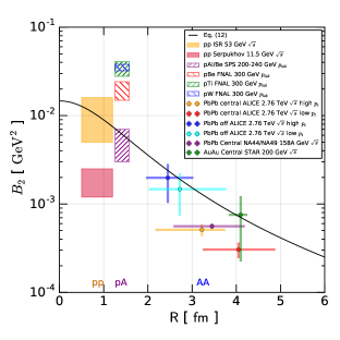
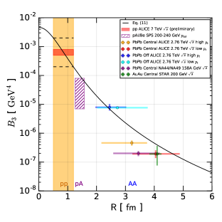
Figure 17: Coalescence factor $B_{2}$ (Left) and $B_{3}$ (Right) vs. HBT radius. For more details, see Blum et al. (2017a).

Importantly, Fig. 17 challenges the simplifying assumptions, utilised in one form or another in Chardonnet et al. (1997); Duperray et al. (2005); Ibarra and Wild (2013b); Cirelli et al. (2014); Herms et al. (2017), of using the same coalescence parameters for pp and pA collisions, or for $\rm\bar{d}$ and $\overline{\rm{}^{3}He}$ production. In particular, $\overline{\rm{}^{3}He}$ coalescence may well be more efficient than priviously estimated in these reference.

We can form a new estimate of $\overline{\rm{}^{3}He}$ production, and put the $\rm\bar{d}$ estimate in possibly useful context, by referring to Fig. 17. HBT data for pp collisions Uribe et al. (1994); Malinina (2013); Aamodt et al. (2010) suggest $R$ in the range $0.5-1.2$ fm, indicated by letters in both panels of Fig. 17. For $pp\to\rm\bar{d}$, direct measurements from the ISR Albrow et al. (1975); Alper et al. (1973); Henning et al. (1978) give

$$B_{2}^{(pp)} = (0.5-1.6)\times 10^{-2}~{}{\rm GeV^{2}}.$$ (36)

For $pp\to\overline{\rm{}^{3}He}$ no direct experimental information is available to date. We extract a rough prediction of $B_{3}$, by taking the intersect of Eq. (35), as realised in Scheibl and Heinz (1999), with the two ends of the relevant range for $R$. This gives the following order of magnitude estimate:

$$B_{3}^{(pp)} = (2-20)\times 10^{-4}~{}{\rm GeV^{4}}\;\;\,{\rm(HBT-\,based)},$$ (37)

marked by the two horizontal dashed lines in the right panel of Fig. 17.

The $\rm\bar{d}$ and $\overline{\rm{}^{3}He}$ flux obtained with Eqs. (36-37) and the grammage formalism of Eq. (1) are shown as shaded bands in the left and right panels of Fig. 16, respectively.

Very recently ALICE analysis for pp collisions at $\sqrt{s}=13$ TeV was shown to reproduce $B_{2}^{(pp)}\approx 1.6\times 10^{-2}$ GeV², in agreement with Eq. (36) and in support of the idea that the coalescence factor extracted at LHC energy can be usefully extrapolated to much lower CME.

Results from ALICE Sharma (2011) at $\sqrt{s}=7$ TeV pp collisions were analysed in Blum et al. (2017a), and allow a preliminary test of Eq. (37), indicating a consistent coalescence factor $B^{(pp)}_{3}\approx(5-8)\times 10^{-4}$ GeV⁴. A dedicated analysis by the ALICE collaboration is highly motivated and results are expected in the near future. LHCb Alves et al. (2008) is also conducting promising analyses of composite nuclei formation.

V Summary

We reviewed the theoretical interpretation of recent measurements of CR antimatter $\bar{p}$ and $e^{+}$, along with some expected upcoming attempts to detect $\rm\bar{d}$ and $\overline{\rm{}^{3}He}$. While CR antimatter is a promising discovery tool for new physics or exotic astrophysical phenomena, an irreducible background arises from secondary production by primary CR collisions with interstellar matter. Understanding this irreducible background or constraining it from first principles is an interesting challenge.

The state of the art cosmic ray measurements, currently dominated by results from the AMS-02 experiment Aguilar et al. (2013, 2016a); Ting , lead to the following conclusions.

• CR $\bar{p}$ are most likely secondary, coming from CR-gas collisions. This conclusion is based on comparison of the flux of secondary CR boron (B) and $\bar{p}$. The $\bar{p}$ and B fluxes are both consistent with secondary production due to primary CRs traversing the same amount of ISM column density. Variations to this simple picture, due e.g. to non-uniform CR elemental composition at the secondary production sites, are still possible but constrained by the data to the $\mathcal{O}(10\%)$ level. A key uncertainty in the analysis is due to the scarcity of high energy nuclear fragmentation cross section data, that is required for extracting the traversed column density and where all current astrophysical analyses are based on extrapolation from low energies.

• CR $e^{+}$ data is consistent with the same secondary production mechanism responsible for $\bar{p}$. AMS02 measurements of the $e^{+}/\bar{p}$ ratio reveal that this ratio is always below; comparable to; and saturates at high energy the ratio of the secondary production rates $Q_{e^{+}}/Q_{\bar{p}}$, describing the branching fraction for $e^{+}$ and $\bar{p}$ production in proton-ISM collisions. Given that $\bar{p}$ are secondary or at least dominated by secondary production, it appears natural to conclude that $e^{+}$ are also secondary. The alternative hypothesis – models for primary $e^{+}$ such as dark matter annihilation or pulsars – must attribute the coincidence of $e^{+}/\bar{p}$ with the secondary $Q_{e^{+}}/Q_{\bar{p}}$ to a fine-tuned accident involving unrelated free model parameters. Secondary $e^{+}$ would imply that the CR propagation time $t_{\rm esc}$ scales differently with CR rigidity than does the CR grammage $X_{\rm esc}$, and is not much larger than 1 Myr at $\mathcal{R}\gtrsim 100$ GV, suggesting that assumptions made in the context of common phenomenological diffusion models are incorrect. Existing radioactive nuclei data from HEAO3 are consistent with secondary $e^{+}$, and improved upcoming measurements by AMS02 would test the interpretation further.

• The flux of secondary high energy $\overline{\rm{}^{3}He}$ may be observable with a few years exposure of AMS-02. An indirect combined analysis of a large set of high energy accelerator data on pp, pA, and AA collisions suggests that the cross section for $pp\to\overline{\rm{}^{3}He}$ is larger than was estimated in most earlier CR literature, by a factor of 10-100. More direct measurements are expected soon from the LHC collaborations, notably ALICE and LHCb. If true, this analysis predicts the detection of secondary $\overline{\rm{}^{3}He}$ events in 5-10 years exposure of AMS02. Secondary $\overline{\rm{}^{3}He}$ events are constrained to high energy: no secondary event should be seen below $\sim 1$ GeV/nuc. At the time of writing this review, preliminary reports by the AMS02 collaboration hint to a possible positive detection, but the analysis is not background-free and conclusive results are not yet available.

Acknowledgments. KB and RS are supported by the I-CORE program of the Planning and Budgeting Committee and the Israel Science Foundation (grant number 1937/12) and by grant 1507/16 from the Israel Science Foundation. KB is incumbent of the Dewey David Stone and Harry Levine career development chair.

Appendix A Physical meaning of the CR grammage

The cosmic ray grammage $X_{\rm esc}$ (in units of column density) is a useful object for calculating the flux of relativistic, stable, secondary CR nuclei like B, sub-Fe, and $\bar{p}$. For these secondary nuclei, the following formula gives an empirical description of a large set of CR data Binns et al. (1988); Engelmann et al. (1990); Jones et al. (2001); Webber et al. (2003):

$$n_{i}(\mathcal{R})=Q_{i}(\mathcal{R})\,X_{\rm esc}(\mathcal{R}),$$ (38)

where $Q_{i}$ is the local net source (production - losses) for species $i$ per unit column density traversed. Importantly, $X_{\rm esc}$ is a universal function of rigidity and does not carry the species label $i$.

Eq. (38) has become known in the literature as the “leaky box equation”, and is often confused with the so-called leaky box model, which is a simplistic model of CR propagation in which the density of CRs and the density of ISM are assumed to be distributed uniformly in the propagation region. However, Eq. (38) is more general and applies to a broad class of propagation models, of which the leaky box model is just one example. Equally good examples of models that realize Eq. (38) are the commonly adopted steady-state homogeneous diffusion models where the CRs are assumed to diffuse in a large halo of rigidity-independent scale height $L$, enclosing a thinner Galactic gas disc of scale height $h\ll L$. As we show below, neither steady-state, nor diffusion (homogeneous or otherwise) nor special boundary conditions are required in order for Eq. (38) to apply. Needless to say, having verified Eq. (38) observationally, one cannot deduce that any of the above simplifying assumptions applies in Nature.

A sufficient condition for Eq. (38) to apply, is that the relative composition (not the density) of the CRs and the ISM be uniform in the time and place in the Galaxy at which secondary CRs are dominantly produced and from which they arrive to our time and place in the Galactic disc [denoted in what follows by $(\vec{r}_{\odot},t_{\odot})$] Katz et al. (2010). Various propagation models in the literature satisfy this condition to good a approximation.

To make things concrete we focus first on CR boron (B). The net source for B, defined at an arbitrary point $(\vec{r},t)$ in the Galaxy, is

$$Q_{B}(\mathcal{R},\vec{r},t)=\sum_{i={\rm C,N,O,...}}\left(\frac{\sigma_{i\to{\rm B}}}{m_{\rm ISM}}\right)n_{i}(\mathcal{R},\vec{r},t)-\left(\frac{\sigma_{\rm B}}{m_{\rm ISM}}\right)n_{B}(\mathcal{R},\vec{r},t).$$ (39)

Here $m_{\rm ISM}$ is the average mass per ISM particle (for 90%H+10%He we have $m_{\rm ISM}=1.3~{}m_{p}$, where $m_{p}=1.67\times 10^{-24}$ g); $\sigma_{i\to{\rm B}}$ is the cross section for nucleus species $i$ to scatter on ISM particles and fragment into B; $\sigma_{\rm B}$ is the total fragmentation cross section of B. We have suppressed the energy dependence of the cross sections, taking the produced B in the reaction $i\to{\rm B}$ to inherit the rigidity of the parent CR $i$. Note that the energy dependence of the cross section could become important, particularly so when we will come to apply our results to secondary $\bar{p}$. There, we will need to generalise Eq. (39) as applied to $\bar{p}$ production. We will come back to this point later on; for now let us assume that, as in Eq. (39), we can describe the production of secondary CR at rigidity $\mathcal{R}$ by an effective cross section $\sigma$ multiplied by the primary CR particle density taken at the same rigidity $\mathcal{R}$.

The net source, Eq. (39), accounts for fragmentation losses and not only for the production of the secondaries. This allows us to isolate the effect of propagation and put different secondary CR species on equal grounds even if their fragmentation cross sections are different, as is the case for B, sub-Fe, and $\bar{p}$. Upon traversing some volume element in the ISM, located around some point $(\vec{r},t)$ with column density $dX$, the flux of B is augmented by a contribution $J_{\rm B}(\mathcal{R},\vec{r}+d\vec{r},t+dt)=J_{\rm B}(\mathcal{R},\vec{r},t)+Q_{\rm B}(\mathcal{R},\vec{r},t)\,dX$. This is illustrated in Fig. 18.

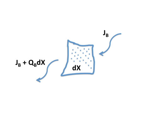
Figure 18: Meaning of the net source $Q_{B}(\mathcal{R},\vec{r},t)$.

To obtain the density of secondary CRs here and now, we sum the contributions $Q\,dX$ of volume elements throughout the Galaxy, weighted by the probability $P\left(\mathcal{R},\{\vec{r},t\},\{\vec{r}_{\odot},t_{\odot}\}\right)$ of a CR with rigidity $\mathcal{R}$, produced at $(\vec{r},t)$, to arrive to us at $(\vec{r}_{\odot},t_{\odot})$, omitting fragmentation loss. Because our use of the net source $Q$ instructs us to omit explicit fragmentation loss in $P$, and because propagation in a magnetic field depends only on the CR rigidity $\mathcal{R}$, we deduce that $P$ does not carry a species label and should apply equally well to B, sub-Fe, or $\bar{p}$. The locally measured density of B, $n_{\rm B}(\mathcal{R},\vec{r}_{\odot},t_{\odot})$, is therefore given by the expression:

$$n_{\rm B}(\mathcal{R},\vec{r}_{\odot},t_{\odot})=\int dt\int d^{3}r\,c\,\rho_{\rm ISM}(\vec{r},t)\,Q_{\rm B}(\mathcal{R},\vec{r},t)\,P\left(\mathcal{R},\{\vec{r},t\},\{\vec{r}_{\odot},t_{\odot}\}\right).$$ (40)

Scaling out the locally measured net production rate, and highlighting the role of the local CR density in the integrand [that we choose to show by the ratio of the density of carbon (C) at the point $(\vec{r},t)$ compared to the locally measured value at $(\vec{r}_{\odot},t_{\odot})$], we have

$$\frac{n_{\rm B}(\mathcal{R},\vec{r}_{\odot},t_{\odot})}{Q_{\rm B}(\mathcal{R},\vec{r}_{\odot},t_{\odot})} = \int dt\int d^{3}r\,c\,\rho_{\rm ISM}(\vec{r},t)\,\frac{n_{\rm C}(\mathcal{R},\vec{r},t)}{n_{\rm C}(\mathcal{R},\vec{r}_{\odot},t_{\odot})}\,P\left(\mathcal{R},\{\vec{r},t\},\{\vec{r}_{\odot},t_{\odot}\}\right)$$ (41)

$$\times \frac{Q_{\rm B}(\mathcal{R},\vec{r},t)/n_{\rm C}(\mathcal{R},\vec{r},t)}{Q_{\rm B}(\mathcal{R},\vec{r}_{\odot},t_{\odot})/n_{\rm C}(\mathcal{R},\vec{r}_{\odot},t_{\odot})}.$$

Let us examine the last factor in the integrand in Eq. (41):

$$\frac{Q_{\rm B}(\mathcal{R},\vec{r},t)/n_{\rm C}(\mathcal{R},\vec{r},t)}{Q_{\rm B}(\mathcal{R},\vec{r}_{\odot},t_{\odot})/n_{\rm C}(\mathcal{R},\vec{r}_{\odot},t_{\odot})} = \frac{\sum_{i={\rm C,N,O,...}}\left(\frac{\sigma_{i\to{\rm B}}}{m_{\rm ISM}}\right)\frac{n_{i}(\mathcal{R},\vec{r},t)}{n_{\rm C}(\mathcal{R},\vec{r},t)}-\left(\frac{\sigma_{\rm B}}{m_{\rm ISM}}\right)\frac{n_{B}(\mathcal{R},\vec{r},t)}{n_{\rm C}(\mathcal{R},\vec{r},t)}}{\sum_{i={\rm C,N,O,...}}\left(\frac{\sigma_{i\to{\rm B}}}{m_{\rm ISM}}\right)\frac{n_{i}(\mathcal{R},\vec{r}_{\odot},t_{\odot})}{n_{\rm C}(\mathcal{R},\vec{r}_{\odot},t_{\odot})}-\left(\frac{\sigma_{\rm B}}{m_{\rm ISM}}\right)\frac{n_{B}(\mathcal{R},\vec{r}_{\odot},t_{\odot})}{n_{\rm C}(\mathcal{R},\vec{r}_{\odot},t_{\odot})}}.$$ (42)

Uniform CR composition means that the ratio $\frac{n_{i}(\mathcal{R},\vec{r},t)}{n_{\rm C}(\mathcal{R},\vec{r},t)}$, while it depends on the species labels $i$ and C, and on rigidity $\mathcal{R}$, does not depend on the point $(\vec{r},t)$. We see that if the CR composition is uniform in the time and place in the Galaxy in which the integrand in Eq. (41) receives most of it’s support, then we can set

$$\frac{Q_{\rm B}(\mathcal{R},\vec{r},t)/n_{\rm C}(\mathcal{R},\vec{r},t)}{Q_{\rm B}(\mathcal{R},\vec{r}_{\odot},t_{\odot})/n_{\rm C}(\mathcal{R},\vec{r}_{\odot},t_{\odot})}=1.$$ (43)

In addition, we may write $n_{C}(\mathcal{R},\vec{r},t)/n_{C}(\mathcal{R},\vec{r}_{\odot},t_{\odot})=n_{\rm CR}(\mathcal{R},\vec{r},t)/n_{\rm CR}(\mathcal{R},\vec{r}_{\odot},t_{\odot})$, where by $n_{\rm CR}(\mathcal{R},\vec{r},t)/n_{\rm CR}(\mathcal{R},\vec{r}_{\odot},t_{\odot})$ we refer collectively to the density contrast of CRs of all species at point $(\vec{r},t)$ compared to their density here at $(\vec{r}_{\odot},t_{\odot})$. Plugging these results into Eq. (41) we find, finally,

$$n_{\rm B}(\mathcal{R},\vec{r}_{\odot},t_{\odot})=Q_{\rm B}(\mathcal{R},\vec{r}_{\odot},t_{\odot})\,X_{\rm esc}(\mathcal{R}),$$ (44)

which coincides with Eq. (38) and identifies $X_{\rm esc}$:

$$X_{\rm esc}(\mathcal{R})\equiv\int dt\int d^{3}r\,c\,\rho_{\rm ISM}(\vec{r},t)\,\frac{n_{\rm CR}(\mathcal{R},\vec{r},t)}{n_{\rm CR}(\mathcal{R},\vec{r}_{\odot},t_{\odot})}\,P\left(\mathcal{R},\{\vec{r},t\},\{\vec{r}_{\odot},t_{\odot}\}\right).$$ (45)

We now get back to the issue of energy dependent fragmentation cross sections. For high energy ($E\gtrsim 10$ GeV/nuc) nuclei, fragmentation is dominated by processes in which a parent nucleus loses an $\alpha$ particle or a few (dominantly one) nuclei. In this process, to a good approximation, the Lorentz factor $\Gamma$ of the parent nucleus is inherited by the leading daughter nucleus – this is the straight-ahead approximation. Since, for the nuclei in question, $A\approx 2Z$ to about 10% accuracy, the magnetic rigidity $\mathcal{R}$ is also inherited by the daughter nucleus to $\mathcal{O}(10\%)$ accuracy. Extending the analysis to CR $\bar{p}$, where the main production cross section $pp\to\bar{p}$ exhibits nontrivial kinematic dependence, is straightforward but introduces sensitivity to the proton spectrum in the secondary production regions. This was discussed in Sec. II.2.

Early analyses Binns et al. (1988); Engelmann et al. (1990); Jones et al. (2001); Webber et al. (2003) relying on HEAO3 data Engelmann et al. (1990) determined the value of $X_{\text{esc}}$ up to $\mathcal{R}\sim 300$ GV. Using recent AMS02 B/C data AMS (2013) to extract the value of $X_{\text{esc}}$ up to $\mathcal{R}=1$ TV, Ref. Blum et al. (2013) derived an approximate power law fit,

$$X_{\rm esc}=8.7\left(\frac{\mathcal{R}}{10~{}{\rm GV}}\right)^{-0.4}\,{\rm g\,cm^{-2}},$$ (46)

consistent at lower energy but slightly harder in slope than deduced from the earlier data Binns et al. (1988); Engelmann et al. (1990); Jones et al. (2001); Webber et al. (2003). This result was later extended directly from data in our evaluation of Eq. (46) as shown in the right panel of Fig. 1.

Appendix B Radiative energy loss of $e^{+}$ vs. CR propagation time: model examples

The detailed interpretation of the form of the $e^{+}$ loss suppression factor $f_{e^{+}}$ is model-dependent. To demonstrate this point, we calculate $f_{e^{+}}$ for two propagation model examples.

First, we consider a version of the leaky-box model (LBM). In this model we assume that the CR density is homogeneous inside some propagation volume $V_{CR}$, containing the MW gas disc and possibly extending some (possibly large) distance above it. We assume that CRs are trapped in $V_{CR}$ for a rigidity dependent time $t^{\rm LBM}_{\rm esc}(\mathcal{R})\propto\mathcal{R}^{-\delta}$ before they escape, and that the average ISM mass density in the propagation region is $\langle\rho_{ISM}\rangle$. We assume that $V_{CR}$ itself is rigidity-independent, so $\langle\rho_{ISM}\rangle$ is also rigidity-independent.

Second we consider a one-dimensional thin disc+halo homogeneous diffusion model, with diffusion coefficient $K(\mathcal{R})\propto\mathcal{R}^{\delta}$ inside a CR propagation region extending to a distance $L$ above and below the gas disc of half-width $h\ll L$. We assume free escape boundary conditions at $z=\pm L$, and again assume that $L$ is rigidity-independent.

Both propagation models satisfy Eq. (1). Therefore calibrating the free parameters in either model (that is, the function $t^{\rm LBM}_{\rm esc}(\mathcal{R})$ and the quantity $\langle\rho_{ISM}\rangle$ for the LBM, or the function $K(\mathcal{R})$ and the quantity $L$ in the diffusion model) to fit the measured B/C, results automatically in a consistent prediction for $\bar{p}/p$ as seen in Fig. 2. We can calculate $X_{\rm esc}$:

$$X_{\rm esc}^{\rm LBM}(\mathcal{R}) = \langle\rho_{ISM}\rangle c\,t^{\rm LBM}_{\rm esc}(\mathcal{R}),$$ (47)

$$X_{\rm esc}^{\rm diff}(\mathcal{R}) = X_{\rm disc}\frac{L\,c}{2K(\mathcal{R})}=\frac{X_{\rm disc}\,c}{L}\,t_{\rm esc}^{\rm diff}(\mathcal{R}).$$ (48)

Here $X_{\rm disc}=2h\rho_{ISM}$ is the grammage of the gas disc, and we define the CR propagation time for the diffusion model:

$$t_{\rm esc}^{\rm diff}(\mathcal{R}) = \frac{L^{2}}{2K(\mathcal{R})}.$$ (49)

Turning to the $e^{+}$ loss suppression factor, we find

$$f_{e+}^{\rm LBM}(\mathcal{R}) = \frac{t_{\rm cool}(\mathcal{R})}{t_{\rm esc}(\mathcal{R})}\int_{1}^{\infty}dxx^{-\gamma_{i}}\exp\left[-\frac{t_{\rm cool}(\mathcal{R})}{t_{\rm esc}(\mathcal{R})}\frac{1-x^{\delta-1}}{1-\delta}\right]$$ (50)

$$\longrightarrow \frac{1}{\gamma_{i}-1}\frac{t_{\rm cool}(\mathcal{R})}{t_{\rm esc}(\mathcal{R})},$$

$$f_{e+}^{\rm diff}(\mathcal{R}) = \sqrt{\frac{t_{\rm cool}(\mathcal{R})}{t_{\rm esc}(\mathcal{R})}}\sqrt{\frac{1-\delta}{\pi}}\int_{1}^{\infty}dx\frac{x^{-\gamma_{i}}}{\sqrt{1-x^{\delta-1}}}\sum_{m=-\infty}^{\infty}(-1)^{m}\exp\left[-\frac{1-\delta}{1-x^{\delta-1}}\frac{t_{\rm cool}(\mathcal{R})}{t_{\rm esc}(\mathcal{R})}m^{2}\right]$$ (51)

$$\longrightarrow \sqrt{\frac{t_{\rm cool}(\mathcal{R})}{t_{\rm esc}(\mathcal{R})}}C_{\rm diff}(\gamma_{i},\delta),\;\;\;C_{\rm diff}(2.7,0.4)\approx 0.8,$$

where we assumed that $t_{\rm cool}\propto\mathcal{R}^{-1}$, and that the $e^{+}$ are produced by a power-law population of protons with spectral index $\gamma_{i}$. The asymptotic behaviour at strong loss (obtained for $t_{\rm cool}\ll t_{\rm esc}$ Katz et al. (2010)) is highlighted in the second line for each model.

While the diffusion model and the LBM differ in the form of $f_{e^{+}}$ they predict, both models share a common feature: because the LBM volume $V_{CR}$ was taken to be rigidity-independent, so is the average ISM density $\langle\rho_{ISM}\rangle$ explored by the CRs and thus $X_{\rm esc}^{\rm LBM}(\mathcal{R})\propto t_{\rm esc}^{\rm LBM}(\mathcal{R})$. Similarly, because the diffusion halo boundary $L$ in the diffusion model was taken to be rigidity independent, also here $X_{\rm esc}^{\rm diff}(\mathcal{R})\propto t_{\rm esc}^{\rm diff}(\mathcal{R})$. In other words: in both of the models, the rigidity-dependent column density of ISM traversed by CRs, is proportional to the rigidity-dependent CR propagation time.

References

- Ginzburg and Ptuskin (1976) V. Ginzburg and V. Ptuskin, Rev.Mod.Phys. 48, 161 (1976).
- Ginzburg et al. (1990) V. Ginzburg, V. Dogiel, V. Berezinsky, S. Bulanov, and V. Ptuskin (1990).
- Longair (1992) M. S. Longair, ed., High-energy astrophysics. Vol. 1: Particles, photons and their detection (1992).
- Kulsrud (2005) R. M. Kulsrud, Plasma physics for astrophysics (2005).
- (5) T. K. Gaisser, R. Engel, and E. Resconi, Cosmic Rays and Particle Physics (Cambridge University Press, ????), ISBN 9780521016469, URL http://www.cambridge.org/de/academic/subjects/physics/cosmology-relativity-and-gravitation/cosmic-rays-and-particle-physics-2nd-edition?format=HB.
- Schlickeiser (2002) R. Schlickeiser, Cosmic ray astrophysics (2002).
- Strong et al. (2007) A. W. Strong, I. V. Moskalenko, and V. S. Ptuskin, Ann. Rev. Nucl. Part. Sci. 57, 285 (2007), eprint astro-ph/0701517.
- Adriani et al. (2009) O. Adriani et al. (PAMELA Collaboration), Nature 458, 607 (2009), eprint 0810.4995.
- Adriani et al. (2010) O. Adriani, G. Barbarino, G. Bazilevskaya, R. Bellotti, M. Boezio, et al., Astropart.Phys. 34, 1 (2010), eprint 1001.3522.
- Adriani et al. (2013a) O. Adriani, G. Bazilevskaya, G. Barbarino, R. Bellotti, M. Boezio, et al., JETP Lett. 96, 621 (2013a).
- Abdo et al. (2009) A. A. Abdo et al. (Fermi-LAT), Phys. Rev. Lett. 102, 181101 (2009), eprint 0905.0025.
- Ackermann et al. (2012a) M. Ackermann et al. (Fermi LAT Collaboration), Phys.Rev.Lett. 108, 011103 (2012a), eprint 1109.0521.
- Ackermann et al. (2010) M. Ackermann et al. (Fermi LAT Collaboration), Phys.Rev. D82, 092004 (2010), eprint 1008.3999.
- Chang et al. (2008) J. Chang et al., Nature 456, 362 (2008).
- Aharonian et al. (2008) F. Aharonian et al. (H.E.S.S.), Phys. Rev. Lett. 101, 261104 (2008), eprint 0811.3894.
- Aharonian et al. (2009) F. Aharonian et al. (H.E.S.S.), Astron. Astrophys. 508, 561 (2009), eprint 0905.0105.
- Aguilar et al. (2013) M. Aguilar, G. Alberti, B. Alpat, A. Alvino, G. Ambrosi, K. Andeen, H. Anderhub, L. Arruda, P. Azzarello, A. Bachlechner, et al. (AMS Collaboration), Phys. Rev. Lett. 110, 141102 (2013), URL http://link.aps.org/doi/10.1103/PhysRevLett.110.141102.
- Aguilar et al. (2016a) M. Aguilar et al. (AMS), Phys. Rev. Lett. 117 (2016a).
- (19) S. Ting (????), URL https://indico.cern.ch/event/592392/.
- Marrocchesi (2016) P. S. Marrocchesi (CALET), J. Phys. Conf. Ser. 718, 052023 (2016).
- Wang et al. (2016) C. Wang et al. (2016), eprint 1604.03219.
- Vandenbroucke et al. (2016) J. Vandenbroucke, P. Karn, M. Wood, and P. Colin (CTA), PoS ICRC2015, 799 (2016), eprint 1509.02480.
- Giovacchini and Choutko (2007) F. Giovacchini and V. Choutko (AMS), in Proceedings, 30th International Cosmic Ray Conference (ICRC 2007): Merida, Yucatan, Mexico, July 3-11, 2007 (2007), vol. 4, pp. 765–768, URL http://indico.nucleares.unam.mx/contributionDisplay.py?contribId=1112&confId=4.
- (24) A. Kounine (AMS), in Proceedings, 32nd International Cosmic Ray Conference (ICRC 2011): Beijing, China, August 11-18, 2011 (????), vol. c, p. 5, URL https://inspirehep.net/record/1352202/files/vc_I02.pdf.
- von Doetinchem et al. (2016) P. von Doetinchem, T. Aramaki, S. Boggs, H. Fuke, C. Hailey, I. Mognet, R. A. Ong, K. Perez, and J. Zweerink, PoS ICRC2015, 1219 (2016), [34,1218(2015)], eprint 1507.02717.
- Aramaki et al. (2016a) T. Aramaki, C. J. Hailey, S. E. Boggs, P. von Doetinchem, H. Fuke, S. I. Mognet, R. A. Ong, K. Perez, and J. Zweerink, Astropart. Phys. 74, 6 (2016a), eprint 1506.02513.
- Abe et al. (2012) K. Abe et al., Phys. Rev. Lett. 108, 051102 (2012), eprint 1107.6000.
- Abe et al. (2012) K. Abe, H. Fuke, S. Haino, T. Hams, M. Hasegawa, A. Horikoshi, A. Itazaki, K. C. Kim, T. Kumazawa, A. Kusumoto, et al., Physical Review Letters 108, 131301 (2012), eprint 1201.2967.
- Di Sciascio and Iuppa (2014) G. Di Sciascio and R. Iuppa (2014), eprint 1407.2144.
- Engelmann et al. (1990) J. Engelmann, P. Ferrando, A. Soutoul, P. Goret, and E. Juliusson, Astron.Astrophys. 233, 96 (1990).
- Webber et al. (2003) W. R. Webber, F. B. McDonald, and A. Lukasiak, Astrophys. J. 599, 582 (2003).
- Katz et al. (2010) B. Katz, K. Blum, J. Morag, and E. Waxman, Mon.Not.Roy.Astron.Soc. 405, 1458 (2010), eprint 0907.1686.
- Ptuskin et al. (1996) V. S. Ptuskin, F. C. Jones, and J. F. Ormes, Astrophys. J. 465, 972 (1996).
- Stephens and Streitmatter (1998) S. A. Stephens and R. E. Streitmatter, Astrophys. J. 505, 266 (1998).
- Ferriere (2001) K. M. Ferriere, Rev. Mod. Phys. 73, 1031 (2001), eprint astro-ph/0106359.
- Gaisser and Schaefer (1992) T. K. Gaisser and R. K. Schaefer, Astrophys. J. 394, 174 (1992).
- Aguilar et al. (2016b) M. Aguilar et al. (AMS), Phys. Rev. Lett. 117, 231102 (2016b).
- Blum et al. (2017a) K. Blum, K. C. Y. Ng, R. Sato, and M. Takimoto (2017a), eprint 1704.05431.
- Tomassetti (2015) N. Tomassetti, Phys. Rev. C92, 045808 (2015), eprint 1509.05776.
- Blum et al. (2013) K. Blum, B. Katz, and E. Waxman, Phys. Rev. Lett. 111, 211101 (2013), eprint 1305.1324.
- Tan and Ng (1983) L. C. Tan and L. K. Ng, Journal of Physics G Nuclear Physics 9, 227 (1983).
- Tan and Ng (1983) L. C. Tan and L. K. Ng, Journal of Physics G: Nuclear Physics 9, 1289 (1983), URL http://stacks.iop.org/0305-4616/9/i=10/a=015.
- Winkler (2017) M. W. Winkler, JCAP 1702, 048 (2017), eprint 1701.04866.
- Aguilar et al. (2015a) M. Aguilar et al. (AMS), Phys. Rev. Lett. 114, 171103 (2015a).
- Aguilar et al. (2015b) M. Aguilar et al. (AMS), Phys. Rev. Lett. 115, 211101 (2015b).
- Yoon et al. (2017) Y. S. Yoon, T. Anderson, A. Barrau, N. B. Conklin, S. Coutu, L. Derome, J. H. Han, J. A. Jeon, K. C. Kim, M. H. Kim, et al., The Astrophysical Journal 839, 5 (2017), URL http://stacks.iop.org/0004-637X/839/i=1/a=5.
- Nozzoli (2016) F. Nozzoli (AMS), in 25th European Cosmic Ray Symposium (ECRS 2016) Turin, Italy, September 04-09, 2016 (2016), eprint 1701.00086, URL https://inspirehep.net/record/1507423/files/arXiv:1701.00086.pdf.
- Cowsik and Burch (2009) R. Cowsik and B. Burch (2009), eprint 0905.2136.
- Burch and Cowsik (2010) B. Burch and R. Cowsik (2010), eprint 1009.1361.
- Cowsik et al. (2014) R. Cowsik, B. Burch, and T. Madziwa-Nussinov, Astrophys. J. 786, 124 (2014), eprint 1305.1242.
- Blasi (2009) P. Blasi, Phys. Rev. Lett. 103, 051104 (2009), eprint 0903.2794.
- Blasi and Serpico (2009) P. Blasi and P. D. Serpico, Phys. Rev. Lett. 103, 081103 (2009), eprint 0904.0871.
- Mertsch and Sarkar (2009) P. Mertsch and S. Sarkar, Phys. Rev. Lett. 103, 081104 (2009), eprint 0905.3152.
- Ahlers et al. (2009) M. Ahlers, P. Mertsch, and S. Sarkar, Phys. Rev. D80, 123017 (2009), eprint 0909.4060.
- Kachelriess et al. (2011) M. Kachelriess, S. Ostapchenko, and R. Tomas, Astrophys. J. 733, 119 (2011), eprint 1103.5765.
- Cholis et al. (2017) I. Cholis, D. Hooper, and T. Linden, Phys. Rev. D95, 123007 (2017), eprint 1701.04406.
- Kachelrie et al. (2015) M. Kachelrie , A. Neronov, and D. V. Semikoz, Phys. Rev. Lett. 115, 181103 (2015), eprint 1504.06472.
- Thomas et al. (2016) B. C. Thomas, E. E. Engler, M. Kachelrie , A. L. Melott, A. C. Overholt, and D. V. Semikoz (2016), [Astrophys. J.826,L3(2016)], eprint 1605.04926.
- Panov et al. (2009) A. Panov, J. Adams, J.H., H. Ahn, G. Bashinzhagyan, J. Watts, et al., Bull.Russ.Acad.Sci.Phys. 73, 564 (2009), eprint 1101.3246.
- Adriani et al. (2011) O. Adriani et al. (PAMELA Collaboration), Science 332, 69 (2011), eprint 1103.4055.
- Adriani et al. (2013b) O. Adriani, G. Barbarino, G. Bazilevskaya, M. Boezio, E. Bogomolov, et al., Adv.Space Res. 51, 219 (2013b).
- Kappl et al. (2015) R. Kappl, A. Reinert, and M. W. Winkler, JCAP 1510, 034 (2015), eprint 1506.04145.
- Donato et al. (2009) F. Donato, D. Maurin, P. Brun, T. Delahaye, and P. Salati, Phys. Rev. Lett. 102, 071301 (2009), eprint 0810.5292.
- Bergstrom et al. (2008) L. Bergstrom, T. Bringmann, and J. Edsjo, Phys. Rev. D78, 103520 (2008), eprint 0808.3725.
- Cholis et al. (2009) I. Cholis, L. Goodenough, D. Hooper, M. Simet, and N. Weiner, Phys. Rev. D80, 123511 (2009), eprint 0809.1683.
- Barger et al. (2009) V. Barger, W. Y. Keung, D. Marfatia, and G. Shaughnessy, Phys. Lett. B672, 141 (2009), eprint 0809.0162.
- Cirelli and Strumia (2008) M. Cirelli and A. Strumia, PoS IDM2008, 089 (2008), eprint 0808.3867.
- Atoyan et al. (1995) A. M. Atoyan, F. A. Aharonian, and H. J. Völk, Phys. Rev. D 52, 3265 (1995), URL https://link.aps.org/doi/10.1103/PhysRevD.52.3265.
- Boulares (1989) A. Boulares, Astrophys. J. 342, 807 (1989).
- Profumo (2011) S. Profumo, Central Eur. J. Phys. 10, 1 (2011), eprint 0812.4457.
- Hooper et al. (2009) D. Hooper, P. Blasi, and P. D. Serpico, JCAP 0901, 025 (2009), eprint 0810.1527.
- Blum et al. (2017b) K. Blum, R. Sato, and M. Takimoto (2017b), eprint 1709.04953.
- Vagelli (2016) V. Vagelli (AMS), PoS ICHEP2016, 070 (2016).
- Lipari (2017) P. Lipari, Phys. Rev. D95, 063009 (2017), eprint 1608.02018.
- Protheroe (1982) R. J. Protheroe, Astrophys. J. 254, 391 (1982).
- Moskalenko and Strong (1998) I. Moskalenko and A. Strong, Astrophys.J. 493, 694 (1998), eprint astro-ph/9710124.
- Delahaye et al. (2009) T. Delahaye, F. Donato, N. Fornengo, J. Lavalle, R. Lineros, P. Salati, and R. Taillet, Astron. Astrophys. 501, 821 (2009), eprint 0809.5268.
- Blumenthal and Gould (1970) G. R. Blumenthal and R. J. Gould, Rev. Mod. Phys. 42, 237 (1970).
- Kappl and Reinert (2017) R. Kappl and A. Reinert, Phys. Dark Univ. 16, 71 (2017), eprint 1609.01300.
- Serpico (2009) P. D. Serpico, Phys. Rev. D79, 021302 (2009), eprint 0810.4846.
- Webber and Soutoul (1998) W. R. Webber and A. Soutoul, Astrophys. J. 506, 335 (1998).
- Shapiro and Silberberg (1970) M. M. Shapiro and R. Silberberg, Annual Review of Nuclear and Particle Science 20, 323 (1970).
- Ptuskin (1999) V. Ptuskin, International Cosmic Ray Conference 4, 195 (1999).
- Simpson, J. A. and Garcia-Munoz, M. (1988) Simpson, J. A. and Garcia-Munoz, M., Space Science Reviews 46, 205 (1988).
- Ptuskin and Soutoul (1998) V. S. Ptuskin and A. Soutoul, Astronomy and Astrophysics 337, 859 (1998).
- Yanasak et al. (2001) N. E. Yanasak, M. E. Wiedenbeck, R. A. Mewaldt, A. J. Davis, A. C. Cummings, J. S. George, R. A. Leske, E. C. Stone, E. R. Christian, T. T. von Rosenvinge, et al., Astrophys. J. 563, 768 (2001).
- Donato et al. (2002) F. Donato, D. Maurin, and R. Taillet, Astron. Astrophys. 381, 539 (2002), eprint astro-ph/0108079.
- Putze et al. (2010) A. Putze, L. Derome, and D. Maurin, Astron. Astrophys. 516, A66 (2010), eprint 1001.0551.
- Blum (2011) K. Blum, JCAP 1111, 037 (2011), eprint 1010.2836.
- Shibata and Ito (2007) T. Shibata and T. Ito, Astrophys. J. 655, 892 (2007).
- Hauser and Dwek (2001) M. G. Hauser and E. Dwek, Ann. Rev. Astron. Astrophys. 39, 249 (2001), eprint astro-ph/0105539.
- Porter and Strong (2005) T. A. Porter and A. Strong (2005), eprint astro-ph/0507119.
- Crutcher et al. (2010) R. M. Crutcher, B. Wandelt, C. Heiles, E. Falgarone, and T. H. Troland, Astrophys. J. 725, 466 (2010).
- Stawarz et al. (2010) L. Stawarz, V. Petrosian, and R. D. Blandford, Astrophys. J. 710, 236 (2010), eprint 0908.1094.
- Shaviv et al. (2009) N. J. Shaviv, E. Nakar, and T. Piran, Phys. Rev. Lett. 103, 111302 (2009), eprint 0902.0376.
- Blandford and Eichler (1987) R. Blandford and D. Eichler, Phys. Rept. 154, 1 (1987).
- Adams et al. (2013) S. M. Adams, C. S. Kochanek, J. F. Beacom, M. R. Vagins, and K. Z. Stanek, Astrophys. J. 778, 164 (2013), eprint 1306.0559.
- Fry et al. (2016) B. J. Fry, B. D. Fields, and J. R. Ellis, Astrophys. J. 827, 48 (2016), eprint 1604.00958.
- Binns et al. (2016) W. R. Binns et al., Science 352, 677 (2016).
- Ackermann et al. (2012b) M. Ackermann et al., Astrophys. J. 756, 4 (2012b), eprint 1207.0616.
- Dermer et al. (2013) C. D. Dermer, A. W. Strong, E. Orlando, and L. Tibaldo (Fermi-LAT), in Proceedings, 33rd International Cosmic Ray Conference (ICRC2013): Rio de Janeiro, Brazil, July 2-9, 2013 (2013), p. 1165, eprint 1307.0497, URL https://inspirehep.net/record/1240658/files/arXiv:1307.0497.pdf.
- Strong (2015) A. W. Strong (Fermi-LAT) (2015), eprint 1507.05006.
- Mizuno et al. (2016) T. Mizuno, S. Abdollahi, Y. Fukui, K. Hayashi, A. Okumura, H. Tajima, and H. Yamamoto, Astrophys. J. 833, 278 (2016), eprint 1610.08596.
- Neronov et al. (2017) A. Neronov, D. Malyshev, and D. V. Semikoz (2017), eprint 1705.02200.
- Malyshev et al. (2009) D. Malyshev, I. Cholis, and J. Gelfand, Phys. Rev. D80, 063005 (2009), eprint 0903.1310.
- Blasi and Amato (2011) P. Blasi and E. Amato, in Proceedings, 1st Session of the Sant Cugat Forum on Astrophysics: High-Energy Emission from Pulsars and their Systems: Sant Cugat, Catalonia, Spain, April 12-16, 2010 (2011), pp. 623–641, eprint 1007.4745, URL https://inspirehep.net/record/863063/files/arXiv:1007.4745.pdf.
- Di Mauro et al. (2014) M. Di Mauro, F. Donato, N. Fornengo, R. Lineros, and A. Vittino, JCAP 1404, 006 (2014), eprint 1402.0321.
- Lee et al. (2011) S. H. Lee, T. Kamae, L. Baldini, F. Giordano, M. H. Grondin, L. Latronico, M. Lemoine-Goumard, C. Sgr , T. Tanaka, and Y. Uchiyama, Astropart. Phys. 35, 211 (2011), eprint 1010.3477.
- Gaskins (2016) J. M. Gaskins, Contemp. Phys. 57, 496 (2016), eprint 1604.00014.
- Meade et al. (2010) P. Meade, M. Papucci, A. Strumia, and T. Volansky, Nucl. Phys. B831, 178 (2010), eprint 0905.0480.
- Cholis and Hooper (2013) I. Cholis and D. Hooper, Phys. Rev. D88, 023013 (2013), eprint 1304.1840.
- Hooper and Tait (2009) D. Hooper and T. M. P. Tait, Phys. Rev. D80, 055028 (2009), eprint 0906.0362.
- Bottino et al. (1998) A. Bottino, F. Donato, N. Fornengo, and P. Salati, Phys. Rev. D58, 123503 (1998), eprint astro-ph/9804137.
- Feng et al. (2001) J. L. Feng, K. T. Matchev, and F. Wilczek, Phys. Rev. D63, 045024 (2001), eprint astro-ph/0008115.
- Donato et al. (2004) F. Donato, N. Fornengo, D. Maurin, and P. Salati, Phys. Rev. D69, 063501 (2004), eprint astro-ph/0306207.
- Bahcall and Soneira (1984) J. N. Bahcall and R. M. Soneira, Astrophys. J. Suppl. 55, 67 (1984).
- Navarro et al. (1996) J. F. Navarro, C. S. Frenk, and S. D. M. White, Astrophys. J. 462, 563 (1996), eprint astro-ph/9508025.
- Merritt et al. (2005) D. Merritt, J. F. Navarro, A. Ludlow, and A. Jenkins, Astrophys. J. 624, L85 (2005), eprint astro-ph/0502515.
- Sellwood (2009) J. A. Sellwood, IAU Symp. 254, 73 (2009), eprint 0807.1973.
- Romano-Diaz et al. (2008) E. Romano-Diaz, I. Shlosman, Y. Hoffman, and C. Heller, Astrophys. J. 685, L105 (2008), eprint 0808.0195.
- Bovy and Tremaine (2012) J. Bovy and S. Tremaine, Astrophys. J. 756, 89 (2012), eprint 1205.4033.
- Jungman et al. (1996) G. Jungman, M. Kamionkowski, and K. Griest, Phys. Rept. 267, 195 (1996), eprint hep-ph/9506380.
- Agashe et al. (2010) K. Agashe, K. Blum, S. J. Lee, and G. Perez, Phys. Rev. D81, 075012 (2010), eprint 0912.3070.
- Bovy (2009) J. Bovy, Phys. Rev. D79, 083539 (2009), eprint 0903.0413.
- Kuhlen and Malyshev (2009) M. Kuhlen and D. Malyshev, Phys. Rev. D79, 123517 (2009), eprint 0904.3378.
- Robertson and Zentner (2009) B. Robertson and A. Zentner, Phys. Rev. D79, 083525 (2009), eprint 0902.0362.
- Feng et al. (2010) J. L. Feng, M. Kaplinghat, and H.-B. Yu, Phys. Rev. Lett. 104, 151301 (2010), eprint 0911.0422.
- Madhavacheril et al. (2014) M. S. Madhavacheril, N. Sehgal, and T. R. Slatyer, Phys. Rev. D89, 103508 (2014), eprint 1310.3815.
- Chan (2015) M. H. Chan, Phys. Rev. D92, 083504 (2015), eprint 1509.06127.
- Ade et al. (2016) P. A. R. Ade et al. (Planck), Astron. Astrophys. 594, A13 (2016), eprint 1502.01589.
- Abdo et al. (2013) A. A. Abdo et al. (Fermi-LAT), Astrophys. J. Suppl. 208, 17 (2013), eprint 1305.4385.
- Goldreich and Julian (1969) P. Goldreich and W. H. Julian, Astrophys. J. 157, 869 (1969).
- Gruzinov (2014) A. Gruzinov (2014), eprint 1402.1520.
- Philippov and Spitkovsky (2017) A. A. Philippov and A. Spitkovsky (2017), eprint 1707.04323.
- Donato et al. (2000) F. Donato, N. Fornengo, and P. Salati, Phys. Rev. D62, 043003 (2000), eprint hep-ph/9904481.
- Baer and Profumo (2005) H. Baer and S. Profumo, JCAP 0512, 008 (2005), eprint astro-ph/0510722.
- Donato et al. (2008) F. Donato, N. Fornengo, and D. Maurin, Phys. Rev. D78, 043506 (2008), eprint 0803.2640.
- Brauninger and Cirelli (2009) C. B. Brauninger and M. Cirelli, Phys. Lett. B678, 20 (2009), eprint 0904.1165.
- Kadastik et al. (2010) M. Kadastik, M. Raidal, and A. Strumia, Phys. Lett. B683, 248 (2010), eprint 0908.1578.
- Cui et al. (2010) Y. Cui, J. D. Mason, and L. Randall, JHEP 11, 017 (2010), eprint 1006.0983.
- Dal and Kachelriess (2012) L. A. Dal and M. Kachelriess, Phys. Rev. D86, 103536 (2012), eprint 1207.4560.
- Ibarra and Wild (2013a) A. Ibarra and S. Wild, JCAP 1302, 021 (2013a), eprint 1209.5539.
- Fornengo et al. (2013) N. Fornengo, L. Maccione, and A. Vittino, JCAP 1309, 031 (2013), eprint 1306.4171.
- Carlson et al. (2014) E. Carlson, A. Coogan, T. Linden, S. Profumo, A. Ibarra, and S. Wild, Phys. Rev. D89, 076005 (2014), eprint 1401.2461.
- Aramaki et al. (2016b) T. Aramaki et al., Phys. Rept. 618, 1 (2016b), eprint 1505.07785.
- Chardonnet et al. (1997) P. Chardonnet, J. Orloff, and P. Salati, Phys. Lett. B409, 313 (1997), eprint astro-ph/9705110.
- Duperray et al. (2005) R. Duperray, B. Baret, D. Maurin, G. Boudoul, A. Barrau, L. Derome, K. Protasov, and M. Buenerd, Phys. Rev. D71, 083013 (2005), eprint astro-ph/0503544.
- Ibarra and Wild (2013b) A. Ibarra and S. Wild, Phys. Rev. D88, 023014 (2013b), eprint 1301.3820.
- Cirelli et al. (2014) M. Cirelli, N. Fornengo, M. Taoso, and A. Vittino, JHEP 08, 009 (2014), eprint 1401.4017.
- Herms et al. (2017) J. Herms, A. Ibarra, A. Vittino, and S. Wild, JCAP 1702, 018 (2017), eprint 1610.00699.
- Lisa et al. (2005) M. A. Lisa, S. Pratt, R. Soltz, and U. Wiedemann, Ann. Rev. Nucl. Part. Sci. 55, 357 (2005), eprint nucl-ex/0505014.
- Scheibl and Heinz (1999) R. Scheibl and U. W. Heinz, Phys. Rev. C59, 1585 (1999), eprint nucl-th/9809092.
- Butler and Pearson (1963) S. T. Butler and C. A. Pearson, Phys. Rev. 129, 836 (1963).
- Schwarzschild and Zupancic (1963) A. Schwarzschild and C. Zupancic, Phys. Rev. 129, 854 (1963).
- Gutbrod et al. (1976) H. H. Gutbrod, A. Sandoval, P. J. Johansen, A. M. Poskanzer, J. Gosset, W. G. Meyer, G. D. Westfall, and R. Stock, Phys. Rev. Lett. 37, 667 (1976).
- Duperray et al. (2003a) R. P. Duperray, K. V. Protasov, and A. Yu. Voronin, Eur. Phys. J. A16, 27 (2003a), eprint nucl-th/0209078.
- Duperray et al. (2003b) R. P. Duperray, K. V. Protasov, L. Derome, and M. Buenerd, Eur. Phys. J. A18, 597 (2003b), eprint nucl-th/0301103.
- Bond et al. (1977) R. Bond, P. J. Johansen, S. E. Koonin, and S. Garpman, Phys. Lett. B71, 43 (1977).
- Mekjian (1977) A. Mekjian, Phys. Rev. Lett. 38, 640 (1977).
- Csernai and Kapusta (1986) L. P. Csernai and J. I. Kapusta, Phys. Rept. 131, 223 (1986).
- Uribe et al. (1994) J. Uribe et al. (BNL-E766), Phys. Rev. D49, 4373 (1994).
- Malinina (2013) L. V. Malinina (ALICE), in Proceedings, 2nd International Conference on New Frontiers in Physics (ICNFP 2013): Kolymbari, Crete, Greece, August 28-September 5, 2013 (2013), eprint 1312.6937, URL https://inspirehep.net/record/1275331/files/arXiv:1312.6937.pdf.
- Aamodt et al. (2010) K. Aamodt et al. (ALICE), Phys. Rev. D82, 052001 (2010), eprint 1007.0516.
- Albrow et al. (1975) M. Albrow, D. Barber, P. Benz, B. Bošnjaković, J. Brooks, C. Chang, A. Clegg, F. Erné, P. Kooijman, F. Loebinger, et al., Nuclear Physics B 97, 189 (1975), ISSN 0550-3213, URL http://www.sciencedirect.com/science/article/pii/0550321375900309.
- Alper et al. (1973) B. Alper, H. Bogild, P. Booth, F. Bulos, L. J. Carroll, G. von Dardel, G. Damgaard, B. Duff, F. Heymann, J. N. Jackson, et al., Physics Letters B 46, 265 (1973).
- Henning et al. (1978) S. Henning et al. (British-Scandinavian-MIT), Lett. Nuovo Cim. 21, 189 (1978).
- Sharma (2011) N. Sharma (ALICE), J. Phys. G38, 124189 (2011), eprint 1109.4836.
- Alves et al. (2008) A. A. Alves, Jr. et al. (LHCb), JINST 3, S08005 (2008).
- Binns et al. (1988) W. R. Binns, T. L. Garrard, M. H. Israel, M. D. Jones, M. P. Kamionkowski, J. Klarmann, E. C. Stone, and C. J. Waddington, Astrophys. J. 324, 1106 (1988).
- Jones et al. (2001) F. C. Jones, A. Lukasiak, V. Ptuskin, and W. Webber, Astrophys. J. 547, 264 (2001), eprint arXiv:astro-ph/0007293.
- AMS (2013) AMS02 Collaboration, new results presented at ICRC2013; www.ams02.org (2013).