Abstract

We recently formulated a model of the universe based on an underlying W3-symmetry. It allows the creation of the universe from nothing and the creation of baby universes and wormholes for spacetimes of dimension 2, 3, 4, 6 and 10. Here we show that the classical large time and large space limit of these universes is one of exponential fast expansion without the need of a cosmological constant. Under a number of simplifying assumptions our model predicts that w=-1.2 in the case of four-dimensional spacetime. The possibility of obtaining a w-value less than -1 is linked to the ability of our model to create baby universes and wormholes.

1 Introduction

According to observations our universe is presently accelerating. Such an acceleration can be caused by the presence of a cosmological constant. However, the precise origin of such a constant is still unclear. Also, modifications of Einstein’s theory of general relativity without an explicit cosmological term can provide explanations of the acceleration. In this article we propose yet another explanation of the acceleration which is caused by the production of baby universes.

In [1, 2] we have formulated a pre-geometric $W_{3}$-symmetric theory. The operators of this theory are represented in a large Hilbert space and the “Hamiltonian” of this theory has no geometric interpretation and strictly speaking not even an interpretation as a Hamiltonian since we do not yet have a concept of time, and finally there are no coupling constants associated with this algebraic structure which we denote the “$W$-algebra world” (WAW), although admittedly there is not much “world” at this stage. However, the WAW can be written as a direct sum of Hilbert spaces where eigenstates of certain of the $\alpha_{k}$ operators associated with the $W_{3}$ model, coherent states relative to the “absolute vacuum state” of the $W_{3}$ algebra, play the role of physical vacuum states. Projected onto one of the Hilbert spaces associated with these vacua, the $W_{3}$ “Hamiltonian” can be given an interpretation as a real Hamiltonian multiplied by a time-coordinate, and the expectation values of the $\alpha_{k}$ operators associated with the chosen coherent state will define the coupling constants of the Hamiltonian. One can view the choice of a coherent state as a kind of spontaneous symmetry breaking of the $W_{3}$ symmetry which results in the emergence of time and a corresponding Hamiltonian. This Hamiltonian has the potential to spontaneously create “space” from nothing, to evolve space in time and to merge and split such universes.

We will show that under certain assumptions the large time behaviour of our model is that of exponential fast expansion precisely as in the standard $\Lambda$-DCM model, but the origin of the acceleration is not a cosmological constant $\Lambda$, but another parameter we denote $B$, related to the $W_{3}$ symmetry breaking and more specifically to the splitting and merging of spatial universes.

2 The “classical” Hamiltonian

The $W_{3}$-model studied in [1] allows for the creation of a two-dimensional expanding universe from “nothing”. We will first discuss the dynamics of the two-dimensional model and then generalize it to four-dimensional spacetime. Let us briefly describe the two-dimensional model (for details we refer to [1, 2]). A $W_{3}$ algebra is defined in terms of operators $\alpha_{n}$ satisfying

$$[\alpha_{m},\alpha_{n}]=m\,\delta_{m+n,0}.$$ (1)

The so-called $W$-Hamiltonian ${{\hat{H}}}_{\rm W}$ is then defined by

$${{\hat{H}}}_{\rm W}:=-\,\frac{1}{3}\sum_{k,l,m=-2}:\!\alpha_{k}\alpha_{l}\alpha_{m}\!:$$ (2)

where the normal ordering $:\!\!(\cdot)\!\!:$ refers to the $\alpha_{n}$ operators ($\alpha_{n}$ to the left of $\alpha_{m}$ for $n>m$). Note that ${{\hat{H}}}_{\rm W}$ does not contain any coupling constants. The “absolute vacuum” $\left|0\right\rangle$ is defined by:

$$\alpha_{n}|0\rangle=0,\quad n\leq 0.$$ (3)

By introducing a coherent state, which is an eigenstate of $\alpha_{0}$, $\alpha_{-1}$ and $\alpha_{-3}$ and which we denoted the “physical” vacuum state $|{\rm vac}\rangle$, ${{\hat{H}}}_{\rm W}$ is closely related to the so-called generalized causal dynamical triangulation (CDT) string field Hamiltonian ${\hat{H}}$ (see [6] for a definition and details), and the coupling constants of ${\hat{H}}$ are defined via the expectation values of the operators $\alpha_{0}$, $\alpha_{-1}$ and $\alpha_{-3}$. More precisely one has [1]

$${{\hat{H}}}_{\rm W}\propto{\hat{H}}+c_{4}\alpha_{4}+c_{2}\alpha_{2}$$ (4)

where ${\hat{H}}$ is the CDT string field Hamiltonian with standard creation and annihilation operators acting on the physical vacuum state $|{\rm vac}\rangle$, and $c_{4}$ and $c_{2}$ are nonzero constants. This equation shows that the choice of physical vacuum leads to the CDT string field Hamiltonian ${\hat{H}}$ except for the term $c_{4}\alpha_{4}+c_{2}\alpha_{2}$ which will spontaneously create universes of infinitesimal lengths. Let $L$ denote a macroscopic length of a spatial universe (which we assume has the topology of a circle) and let $\Psi^{\dagger}(L)$ be the operator which creates this spatial universe by acting on $|{\rm vac}\rangle$. The relation between $\Psi^{\dagger}(L)$ and the $\alpha_{n}$ are as follows

$$\Psi^{\dagger}(L)=\sum_{l=0}^{\infty}\frac{L^{l}}{l!}\,\alpha_{l},$$ (5)

and one can now express the string field Hamiltonian ${\hat{H}}$ in terms of $\Psi(L)$ and $\Psi^{\dagger}(L)$:

$${\hat{H}}={\hat{H}}_{0}-g\int\!\!\!\int\!dL_{1}dL_{2}\;\Psi^{\dagger}(L_{1})\Psi^{\dagger}(L_{2})\;(L_{1}\!+\!L_{2})\Psi(L_{1}\!+\!L_{2})+\cdots$$ (6)

where ${\hat{H}}_{0}$ is the original CDT Hamiltonian [4] which does not allow for splitting and merging of spatial universes, while the next term describes the splitting of a universe in two (see [6] for the terms indicated by $\cdots$ which contain a term for merging two universes to one and a term which allows a universe of length zero to vanish). The coupling constant $g$ can be expressed in terms of the expectation values of the operators $\alpha_{0}$ and $\alpha_{-3}$. The classical theory based on ${\hat{H}}$, but describing only the time evolution of a single universe, has as dynamical variables $L$ and its conjugate momentum $\Pi$, which have the following Poisson bracket and Hamiltonian

$$\{L\!\;,\Pi\}\,=\,1,$$ (7)

$${\cal H}=NL\bigg{(}\Pi^{2}-\mu+\frac{2g}{\Pi}\bigg{)}.$$ (8)

Here $\mu$-term is a cosmological term (which we later will dispose of) and $N(t)$ is a Lagrange multiplier field, expressing the invariance of the dynamical system under time-reparametrisation. The $g$-term in (8) comes from merging and splitting terms in (6) while the value of $\mu$ is the product of $-2g$ and the expectation values of $\alpha_{-1}$ (see [1] for details). The Hamiltonian (8) differs from the classical limit of ${\hat{H}}_{0}$ [10] by the presence of the $g$-term which, as mentioned, is related to the merging and splitting of spatial universes and thus to the production of baby universes. It is known that the production of baby universes is intimately related to the the fractal structure of spacetime [11] and thus the presence of the $g$-term originates from a genuine quantum gravity effect.

The time dependences of $L$ and $\Pi$ are now given by

$$\dot{L}\! = \!-\,\{{\cal H}\!\;,L\}\,=\,2NL\bigg{(}\Pi-\frac{g}{\Pi^{2}}\bigg{)},$$ (9)

$$\dot{\Pi}\! = \!-\,\{{\cal H}\!\;,\Pi\}\,=\,-\,N\bigg{(}\Pi^{2}-\mu+\frac{2g}{\Pi}\bigg{)}.$$ (10)

We can solve these equations for $\Pi$ by noting that (9) can be written as

$$\frac{\dot{L}}{2g^{1/3}NL}\,=\,\frac{\Pi}{g^{1/3}}-\bigg{(}\frac{g^{1/3}}{\Pi}\bigg{)}^{\!2}.$$ (11)

Thus we find

$$\Pi=\frac{\dot{L}}{2NL}F(x),\qquad\quad x:=-\frac{8gN^{3}L^{3}}{\dot{L}^{3}},$$ (12)

where $F(x)$ satisfies

$$\big{(}F(x)\big{)}^{3}-\big{(}F(x)\big{)}^{2}+x\ =\ 0.$$ (13)

The regions of $x$ and $F$ are $x\leq\frac{4}{27}$ and $F\geq\frac{2}{3}$, respectively, if we start from a universe with zero length. From this we find the Lagrangian

$${\cal L}=-{\cal H}+\Pi\dot{L}=NL\bigg{(}\Pi^{2}+\mu-\frac{4g}{\Pi}\bigg{)},$$ (14)

where $\Pi$ is replaced by the right-hand side of the first equation of (12). Finally the equation which describes the expansion of the universe (our modified Friedmann equation without matter) is

$$\frac{\delta S}{\delta N}=0,\qquad\quad S:=\int\!dt\!\;{\cal L}.$$ (15)

One can show that the other equation of motion, $\delta S/\delta L=0$, is just the time derivative of eq. (15).

3 After the Big Bang

As mentioned above the $W_{3}$-model has the potential to describe how the universe emerges from a pre-geometric theory where there is no interpretation of time and space. Space born with zero length expands its size $L(t)$ as [2]

$$L(t)\approx\frac{1}{\sqrt{\mu}}\tanh(\sqrt{\mu}\,t)\qquad{\rm or}\qquad L(t)\approx\frac{1}{\sqrt{-\mu}}\tan(\sqrt{-\mu}\,t)$$ (16)

depending on the sign of the cosmological constant $\mu$ in (14). We denote this the THT-expansion, referring to the functions appearing in (16). However, this “classical” expansion of space from zero length to a macroscopic size (i.e. a size larger than or equal the Planck length) is complicated by the creation and annihilation of spatial universes dictated by the CDT string field Hamiltonian.

In this article we will be interested in the other limit, that of large time and large space extension and a situation where matter fields are included in the model. In principle one can include matter fields in the string field Hamiltonian, but we here take the phenomenological approach that for large space extensions and large times we insert the classical energy-momentum tensor in the classical equations resulting from (14). Also, we will drop the $\mu$-term in (14) which is like a cosmological term. We will not need it and in [2] we argued that effectively it might be zero by quantum effects caused by wormholes (the Coleman mechanism [12]) when a universe reaches Planck size or larger. We will assume that the $g$-term remains in the macroscopic region, although quantum effects could change its bare value, so we denote the effective macroscopic value $B$. Since $g$ originates from interaction terms in the string field Hamiltonian describing the splitting of a spatial universe in two or the merging of two spatial universes into one, $g$ is also related to the creation of spacetime wormholes and is thus linked to specific geometric properties of spacetime. Therefore it is difficult to imagine that local dynamics effectively can force it to be zero, and the assumption of a non-vanishing $g$-tem in the “classical” hamiltonian (14) is quite natural. Thus effectively we make the replacement $\mu\to\frac{1}{12}\kappa\rho$, $g\to-\frac{1}{8}B$ and with these substitutions we obtain

$$\frac{\delta S}{\delta N}=0,\qquad\quad S:=\int\!dt\!\;{\cal L}\,\Big{|}_{\mu\to\frac{1}{12}\kappa\rho,\,g\to-\frac{1}{8}B},$$ (17)

where $\kappa$ is a positive constant which is proportional to the gravitational constant and $\rho$ is the energy density of matter. This is our modified Friedmann equation. After some algebra it can be written as

$$\frac{\dot{L}^{2}}{N^{2}L^{2}}\,=\,\frac{\kappa\rho}{3}+\frac{BNL}{\dot{L}}\,\frac{1+3F(x)}{\big{(}F(x)\big{)}^{2}},\qquad\quad x:=\frac{BN^{3}L^{3}}{\dot{L}^{3}}.$$ (18)

Making the gauge choice $N(t)=1$ we see that under the assumption that $\rho\to 0$ for $L\to\infty$ we have for large $t$ that $\dot{L}/L$ is constant, and we find

$$\frac{\dot{L}}{L}\to 3\sqrt[3]{B/4},\qquad{\rm i.e.}\qquad L\,\sim\,e^{\,3\sqrt[3]{B/4}\,t}.$$ (19)

This value is also the boundary value $x=\frac{4}{27}$, so the Hubble parameter $H:=\dot{L}/L$ takes values in the region $3\sqrt[3]{B/4}\leq H\leq\infty$. Thus the $B$-term acts effectively as a cosmological term for large $t$ in the sense that it can lead to an exponentially expanding universe for large t.

The two-dimensional $W_{3}$ symmetry breaking scenario was generalized to 3, 4, 6 and 10 dimensional spacetime by considering $W_{3}$ algebras with intrinsic symmetries [2]. Like the ordinary Friedmann equation, which assumes homogeneity and isotropy of space and which is independent of the dimension of space, we expect that our modified Friedmann equation will also be independent of the dimension of space if we make the same assumptions. Here we will concentrate on the four-dimensional spacetime case and thus write the modified Friedmann equation (18) (identifying the conventional scale factor $a(t)$ with $L(t)$ and gauge fixing to $N(t)=1$).

$$\frac{\dot{L}^{2}}{L^{2}}\,=\,\frac{\kappa\rho}{3}+\frac{BL}{\dot{L}}\,\frac{1+3F(x)}{\big{(}F(x)\big{)}^{2}},\qquad\quad\hbox{where}\quad x:=\frac{BL^{3}}{\dot{L}^{3}}.$$ (20)

One quantity in (20) will depend on the dimension of space, namely $\rho$. For simplicity we will here assume we have a simple matter dust system. Thus the pressure of matter is zero and for our three-dimensional space we have

$$\kappa\rho=\frac{C}{L^{3}},\quad\dot{\rho}=-\,3H\rho,\quad H(t):=\frac{\dot{L}}{L},$$ (21)

where $H(t)$ is the usual (time dependent) Hubble parameter and $C$ is a positive constant. On the right-hand side of equation (20), the first term is the matter energy and the second term is a new type of term (we have chosen the cosmological constant $\Lambda=0$ so we do not have a “standard” dark energy term). In order to make clearer the ratio of these “energies”, (20) can be written as

$$\Omega_{\rm m}(t)+\Omega_{B}(t)+\Omega_{K}(t)+\Omega_{\Lambda}(t)\,=\,1,$$ (22)

where

$$\Omega_{\rm m}(t)\,:=\,\frac{\kappa\rho}{3}\bigg{(}\frac{L}{\dot{L}}\bigg{)}^{\!2},\qquad\Omega_{B}(t)\,:=\,\frac{x\big{(}1+3F(x)\big{)}}{\big{(}F(x)\big{)}^{2}},\qquad\Omega_{K}(t)=\Omega_{\Lambda}(t)=0.$$ (23)

In our model the topology of space is toroidal, so the space is flat, i.e. $\Omega_{K}(t)=0$. Moreover, the cosmological constant is assumed to be zero because of the Coleman mechanism, so the dark energy is also zero, i.e. $\Omega_{\Lambda}(t)=0$. We now write the modified Friedmann equation as

$$\frac{\dot{L}^{2}}{L^{2}}\,=\,\frac{C}{3L^{3}}+\frac{4BL}{\dot{L}}+\frac{5B^{2}L^{4}}{\dot{L}^{4}}+\ldots$$ (24)

and solve it perturbatively in $B$, starting with the boundary condition that $L(t)=0$ for $t=0$:

$$L(t)\,=\,\bigg{(}\frac{3C}{4}\bigg{)}^{\!1/3}\bigg{(}t^{2/3}+\frac{9\!\>B\!\>t^{11/3}}{8}-\frac{1539\!\>B^{2}\!\>t^{20/3}}{1792}+\ldots\bigg{)}.$$ (25)

When the time $t$ increases from $0$ to $\infty$, $x$ increases from $0$ to $\frac{4}{27}$ and $F$ decreases from $1$ to $\frac{2}{3}$.

Lastly, we use as observed parameters $t_{0}$, the present age of the universe, and $H_{0}:=H(t_{0})$, the present value of the Hubble parameter. In the standard CDM model $H_{0}$ determines the present age of the universe $t_{0}$. Our model needs one more experimental input besides the present Hubble parameter $H_{0}$ because there exists one more parameter $B$. We here use the present time $t_{0}$ in order to fix the parameter $B$. We choose

$$t_{0}=13.8\,[\,{\rm Gyr}\,],\qquad\quad H_{0}=69\,[\,{\rm km}\,{\rm s}^{-1}\!\;{\rm Mpc}^{-1}\,].$$ (26)

These values of $t_{0}$ and $H_{0}$ are based on the recent observations and determine the function $L(t)$ (25) without ambiguity except for the factor $C$. The graph of $a(t):=L(t)/L(t_{0})$ together with those of the $a(t)$’s of the CDM model and the $\Lambda$-CDM model are shown in Fig. 1.

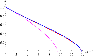
Figure 1: The solid line, the dashed line and the dotted line are $a(t):=\frac{L(t)}{L(t_{0})}$ of our model, the $\Lambda$-CDM model and the CDM model, respectively

One finds that the expansion of the universe as well as the late acceleration in our model is very similar to that in the $\Lambda$-CDM model.

Since $L(t)$’s of our model and the $\Lambda$-CDM model are very similar, we need to distinguish them carefully. Using $L(t)$, we obtain the $\Omega_{\rm m}(t)$, $q(t)$ and $w(t)$ of our model, defined by

$$\Omega_{\rm m}(t)\,:=\,\frac{\kappa\rho}{3}\bigg{(}\frac{L}{\dot{L}}\bigg{)}^{\!2},\qquad q(t):=-\bigg{(}\frac{L}{\dot{L}}\bigg{)}^{\!2}\frac{\ddot{L}}{L},\qquad w(t):=-\,\frac{1-2q}{3\!\>\Omega_{B}},$$ (27)

respectively, and we show the graphs in Figs. 2–4. The $q(t)$ and $w(t)$ of our model are different from $q(t)$ and $w(t)$ of $\Lambda$-CDM model.

Define $\Omega_{{\rm m}0}:=\Omega_{\rm m}(t_{0})$, $q_{0}:=q(t_{0})$ and $w_{0}:=w(t_{0})$, as well as the time $t_{\ast}$ where the acceleration of the universe is zero, defined by $\ddot{L}(t_{\ast})\!=\!0$, and the corresponding value of the red shift $z_{\ast}:=\big{(}L(t_{0})-L(t_{\ast})\big{)}/L(t_{\ast})$. We then obtain

$$\Omega_{{\rm m}0}\sim 0.33,\qquad q_{0}\sim-0.74,\qquad w_{0}\sim-1.2,$$ (28)

$$t_{\ast}\sim 7.8\,[\,{\rm Gyr}\,],\qquad z_{\ast}\sim 0.60.$$ (29)

It is worth noting that the values quoted in (28) and (29) are not very sensitive to the precise values of $H_{0}$ and $t_{0}$ cited in (26). The value of $\Omega_{{\rm m}0}$ of our model is somewhat bigger than the corresponding $\Omega_{{\rm m}0}$ ($\sim 0.29$) of the $\Lambda$-CDM model. The major difference compared to the $\Lambda$-CDM model is that we have a $w_{0}$ value which is less than -1. In the conventional scenarios this is usually only possible if one introduces some kind of ghost fields. However, that is not necessary in our model.

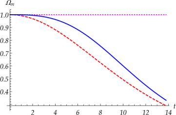
Figure 2: The solid line, the dashed line and the dotted line are $\Omega_{\rm m}(t)$ of our model, the $\Lambda$-CDM model and the CDM model, respectively

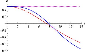
Figure 3: The solid line, the dashed line and the dotted line are $q(t)$ of our model, the $\Lambda$-CDM model and the CDM model, respectively

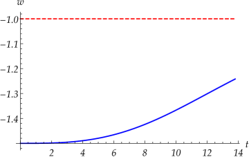
Figure 4: The solid line and the dashed line are $w(t)$ of our model and the $\Lambda$-CDM model, respectively

4 Discussion

We have presented an alternative Friedmann equation where the solution fits the data as well as the ordinary Friedmann equation, but which does not require a cosmological constant in order to produce the presently observed acceleration. Of course various $f(R)$ models of gravity can also lead to acceleration after a matter dominated deceleration and if we only keep the linear term in $B$ in our expansion, one will not be able to distinguish our model from a suitable $f(R)$ model (see [13] for a review of $f(R)$ models). While the deviation of $f(R)$ from the pure Einstein term presently is mainly dictated by the desire to match observations, the origin of the $B$-term in our model is “natural” in the sense that it appears in the $W_{3}$ models for the creation of our universe that we have suggested elsewhere [1, 2].

In this paper we have only dealt with the later times of the universe. We used $a(t)=0$ for $t=0$. But this $t=0$ was only intended to represent a “short” time after the Big Bang and we have made no attempt to follow the detailed history of the universe related a radiation area and a matter dominated area. The reason is that our additional term is not important at early times. However, as reported in [1, 2] our model describes the expansion of the universe from “absolute” zero size and it has the potential to produce an extended universe in a short time scale. The reason we do not present here a continuous time-picture from “absolute” zero time to the present time is that a non-perturbative treatment is needed to understand the full emergence of extended spacetime with a metric from the pre-geometric state of the universe. In this article we assumed that such an extended spacetime have been formed, and we started from there and studied the effect of the new term present in the evolution equations for late times. The obvious next step to be addressed is to understand how the emergence of spacetime from pre-geometry can be matched with the standard inflation picture. Presently our model has nothing to say about the naturalness of the value of $\sqrt[3]{B}\sim 0.49/t_{0}$. Like the cosmological constant $\Lambda$ in the $\Lambda$-CDM model it is mysteriously small compared to the Planck scale. However, since we have not yet connected the sub-Planckian region of our model with the late time region of the model, it is possible that the magnitude of $B$ has a dynamical origin.

Our model clearly allows for more drastic scenarios than just an accelerating universe. It is born with the ability to create baby universes and wormholes, processes which might not only be important when the universe is of Planck size. Clearly it will be of utmost importance to understand how such processes manifest themselves when we already have created a macroscopic universe like the one we inhabit today. If we look at the string field equation for splitting and joining spatial universes and naively assume that it can be applied to three-dimensional spaces, the dynamics of this splitting being driven by the effective coupling constant $B$, then the small value of $B$ that we seemingly observe would indicate that there is only a small chance of splitting our present universe in two. In fact the probability per unit time is more or less equal to the inverse age of our universe. However, since $B$ is only an effective coupling constant, the dynamics could be very different when the universe at Planck time was at Planck size, as already mentioned.

Finally, the selection of a coherent state serving as a physical vacuum, which has been applied to the WAW world, probably has the same features as other more standard scenarios of spontaneous symmetry breaking, e.g. the symmetry breaking of the Standard Model. In the Standard Model the vacuum is a coherent state where the Higgs field has an expectation value different from zero. However, this state may only be meta-stable and if that is the case it can decay to another state where the expectation value of the Higgs field is zero. This would induce an abrupt change in the coupling constants of the Standard Model. Similarly, the coherent state corresponding to one physical vacuum in the WAW could change to another coherent state corresponding to another physical vacuum, thereby inducing an abrupt change in the values of the coupling constants of the string field Hamiltonian. Clearly, these important questions have to be addressed in order understand not only the model, but also its predictive power.

Acknowledgments.

JA and YW acknowledge support from the ERC-Advance grant 291092, “Exploring the Quantum Universe” (EQU). J.A. acknowledge financial support by the Independent Research Fund Denmark through the grant “Quantum Geometry”.

References

- [1] J. Ambjorn and Y. Watabiki, Phys. Lett. B 749 (2015) 149, [arXiv:1505.04353 [hep-th]].
-
[2]
J. Ambjorn and Y. Watabiki,
Phys. Lett. B 770 (2017) 252,
[arXiv:1703.04402 [hep-th]].
Acta Phys. Polon. Supp. 10 (2017) 299, [arXiv:1704.02905 [hep-th]]. -
[3]
L.J. Romans,
Nucl. Phys. B 352 (1991) 829.
N. Mohammedi, Mod. Phys. Lett. A 6 (1991) 2977.
J.M. Figueroa-O’Farrill, Phys. Lett. B 326 (1994) 89, [hep-th/9401108].
S.A. Lyakhovich and A.A. Sharapov, hep-th/9411167.
C.M. Hull, In *Trieste 1992, Proceedings, High energy physics and cosmology* 76-142 and London Queen Mary and Westfield Coll. - QMW-93-02 (93/02) 54 p. (305933) [hep-th/9302110]. - [4] J. Ambjorn and R. Loll, Nucl.Phys.B 536 (1998) 407-434, [hep-th/9805108].
-
[5]
J. Ambjorn, R. Loll, W. Westra and S. Zohren,
JHEP 0712 (2007) 017
[arXiv:0709.2784 [gr-qc]].
J. Ambjorn, R. Loll, Y. Watabiki, W. Westra and S. Zohren, Phys. Lett. B 665 (2008) 252 [arXiv:0804.0252 [hep-th]].
J. Ambjorn, R. Loll, W. Westra and S. Zohren, Phys. Lett. B 678 (2009) 227 [arXiv:0905.2108 [hep-th]].
J. Ambjorn and T. G. Budd, J. Phys. A: Math. Theor. 46 (2013) 315201 [arXiv:1302.1763 [hep-th]]. - [6] J. Ambjorn, R. Loll, Y. Watabiki, W. Westra and S. Zohren, JHEP 0805 (2008) 032 [arXiv:0802.0719 [hep-th]].
-
[7]
N. Ishibashi and H. Kawai,
Phys. Lett. B 314 (1993) 190
[hep-th/9307045].
Phys. Lett. B 322 (1994) 67
[hep-th/9312047].
Phys. Lett. B 352 (1995) 75
[hep-th/9503134].
Y. Watabiki, Nucl. Phys. B 441 (1995) 119 [hep-th/9401096]. Phys. Lett. B 346 (1995) 46 [hep-th/9407058].
J. Ambjorn and Y. Watabiki, Int. J. Mod. Phys. A 12 (1997) 4257 [hep-th/9604067]. - [8] J. Ambjorn, A. Goerlich, J. Jurkiewicz and R. Loll, Phys. Rept. 519 (2012) 127 [arXiv:1203.3591 [hep-th]].
-
[9]
J. Ambjorn, A. Görlich, J. Jurkiewicz and R. Loll,
Phys. Rev. Lett. 100 (2008) 091304 [arXiv:0712.2485, hep-th].
Phys. Rev. D 78 (2008) 063544 [arXiv:0807.4481, hep-th].
Phys. Lett. B 690 (2010) 420-426 [arXiv:1001.4581, hep-th].
J. Ambjorn, J. Jurkiewicz and R. Loll, Phys. Rev. Lett. 93 (2004) 131301 [hep-th/0404156]. Phys. Rev. D 72 (2005) 064014 [hep-th/0505154]. Phys. Lett. B 607 (2005) 205-213 [hep-th/0411152].
J. Ambjorn, A. Gorlich, S. Jordan, J. Jurkiewicz and R. Loll, Phys. Lett. B 690 (2010) 413 [arXiv:1002.3298 [hep-th]].
J. Ambjorn, S. Jordan, J. Jurkiewicz and R. Loll, Phys. Rev. Lett. 107 (2011) 211303 [arXiv:1108.3932 [hep-th]]. Phys. Rev. D 85 (2012) 124044 [arXiv:1205.1229 [hep-th]]. - [10] J. Ambjorn, L. Glaser, Y. Sato and Y. Watabiki, Phys. Lett. B 722 (2013) 172 [arXiv:1302.6359 [hep-th]].
-
[11]
H. Kawai, N. Kawamoto, T. Mogami and Y. Watabiki,
Phys. Lett. B 306 (1993) 19,
[hep-th/9302133].
J. Ambjorn and Y. Watabiki, Nucl. Phys. B 445 (1995) 129, [hep-th/9501049].
J. Ambjorn, J. Jurkiewicz and Y. Watabiki, Nucl. Phys. B 454 (1995) 313, [hep-lat/9507014]. - [12] S. R. Coleman, Nucl. Phys. B 310 (1988) 643.
- [13] T. P. Sotiriou and V. Faraoni, Rev. Mod. Phys. 82 (2010) 451, [arXiv:0805.1726 [gr-qc]].