Atomic Clock Ensemble in Space (ACES) data analysis

Abstract

The Atomic Clocks Ensemble in Space (ACES/PHARAO mission, ESA & CNES) will be installed on board the International Space Station (ISS) next year. A crucial part of this experiment is its two-way MicroWave Link (MWL), which will compare the timescale generated on board with those provided by several ground stations disseminated on the Earth. A dedicated Data Analysis Center (DAC) is being implemented at SYRTE – Observatoire de Paris, where our team currently develops theoretical modelling, numerical simulations and the data analysis software itself.

In this paper, we present some key aspects of the MWL measurement method and the associated algorithms for simulations and data analysis. We show the results of tests using simulated data with fully realistic effects such as fundamental measurement noise, Doppler, atmospheric delays, or cycle ambiguities. We demonstrate satisfactory performance of the software with respect to the specifications of the ACES mission. The main scientific product of our analysis is the clock desynchronisation between ground and space clocks, i.e. the difference of proper times between the space clocks and ground clocks at participating institutes. While in flight, this measurement will allow for tests of General Relativity and Lorentz invariance at unprecedented levels, e.g. measurement of the gravitational redshift at the $3\times 10^{-6}$ level.

As a specific example, we use real ISS orbit data with estimated errors at the 10 m level to study the effect of such errors on the clock desynchronisation obtained from MWL data. We demonstrate that the resulting effects are totally negligible.

¹LNE-SYRTE, Observatoire de Paris, PSL Research University, CNRS, Sorbonne Universités, UPMC Univ. Paris 06, 61 avenue de l’Observatoire, 75014 Paris, France

²Laboratoire Kastler Brossel, ENS-PSL Research University, CNRS, UPMC-Sorbonne Universités, Collège de France, 75005 Paris, France

Contact : Frederic.Meynadier@obspm.fr

September 2017, revised version December 2017

Accepted in Classical and Quantum Gravity, 2018, Volume 35, Number 3 :

https://doi.org/10.1088/1361-6382/aaa279

Keywords: General Relativity, Atomic Clocks, Tests of Fundamental Physics, Relativistic Time and Frequency Transfer, Data Analysis, Space Mission

1 Introduction

The Einstein Equivalence Principle (EEP) is the foundation of General Relativity (GR) and more generally of all metric theories of gravitation [1], and therefore requires extensive experimental verification. Additionally, numerous theories beyond GR that seek to unify gravitation with other fundamental interactions in nature allow for a violation of EEP at some, a priori unknown, level. Although the different aspects of the EEP like the Universality of Free Fall (UFF) or the gravitational redshift of clocks are related [1], that relationship cannot be quantified a priori [2] and therefore they need to be tested independently. UFF is currently being tested at unprecedented uncertainty in the MICROSCOPE space experiment [3] that was launched in 2016. Another famous aspect of the EEP is the gravitational redshift of clocks, that is so far best tested in the Gravity Probe A experiment [4, 5, 6] that used a hydrogen maser onboard a rocket on a parabolic trajectory which was compared via a two-way microwave link to a hydrogen maser on the ground. One of the main scientific objectives of the ACES/PHARAO space mission is to improve on that test by roughly two orders of magnitude.

The ACES/PHARAO mission is an international metrological space mission led by the European Space Agency (ESA) in collaboration with the French Space Agency (Centre National d’Études Spatiales, CNES). It aims at realizing a time scale of high stability and accuracy on board the International Space Station (ISS) using a unique cold-atom space clock developed by CNES in collaboration with LNE-SYRTE, together with a space hydrogen maser (SHM). Additionally, ACES will be equipped with microwave (MWL) and optical (European Laser Timing, ELT) links which will allow frequency/time comparisons between the onboard time scale and time scales on the ground.

The on-board timescale will track the Space Station clock’s proper time, accumulating phase difference with respect to ground-based counterparts as it navigates through the Earth’s gravity potential at orbital speed. Keeping track of proper time differences, i.e. clock desynchronisation, allows to test General Relativity predictions : such tests are then limited by the noise introduced by the clocks and the link between them. In the case of ACES/PHARAO, the MWL has been designed to suit the performance of the space clock during ISS visibility passes.

The clock ensemble relative frequency stability (expressed in Allan deviation, ADEV, see e.g. [7]) should be better than $\sigma_{y}=10^{-13}\cdot\tau^{-1/2}$, which corresponds to $3\times 10^{-16}$ after one day of integration (see figure 2); time deviation (TDEV) should be better than $2.1\times 10^{-14}\cdot\tau^{1/2}$, which corresponds to 12 ps after one day of integration (see figure 2). The fractional frequency uncertainty of the clock ensemble should be around $10^{-16}$. As the expected gravitational frequency shift between ground and space clocks for an ISS altitude of 400 km is around $4\times 10^{-11}$, this is coherent with a measurement of the gravitational redshift at the $3\times 10^{-6}$ level.

Figure 1: Performance objective of the ACES clocks and the ACES space-ground time and frequency transfer expressed in time deviation.

Figure 2: PHARAO (Cesium clock) and SHM (hydrogen maser) expected performances in Allan deviation

The main scientific objectives of this mission are [8, 9]:

• To demonstrate the high performance of the atomic clocks ensemble in the space environment and the ability to achieve high stability on space-ground time and frequency transfer.

• To compare ground clocks at high resolution on a worldwide basis using a link in the microwave domain. In common view mode, the link stability should reach around 0.3 ps after 300 s of integration; in non-common view mode, it should reach a stability of around 7 ps after 1 day of integration (see figure 2).

• To perform equivalence principle tests. It will be possible to test the gravitational redshift with unprecedented accuracy, to carry out novel tests of Lorentz invariance and to contribute to searches for possible variations of fundamental constants.

Besides these primary objectives, several secondary objectives can be found in [10]. For example, comparing distant ground clocks at the $10^{-17}$ uncertainty level in fractional frequency allows the determination of the potential difference between their locations via the gravitational redshift with an uncertainty of about 1 m²/s², corresponding to an uncertainty in height of about 10 cm, a method of geodesy referred to as chronometric geodesy [11, 12, 13, 14].

These science objectives are directly linked to the MWL performance. For example, the short term ($\leq$ 300 s) stability of the MWL directly affects the test of Lorentz invariance [15, 16], or the comparison of ground clocks at the $10^{-17}$ level, which in turn is required to efficiently contribute to searches for the variation of fundamental constants [8]. The test of the gravitational redshift will likely be limited by the long term performance of the MWL and the on-board clocks, but ensuring adequate short term performance of the MWL is essential as well, e.g. for an efficient evaluation of systematic effects.

In this article we describe the operation of the MWL of ACES, with particular emphasis on the theoretical description of the observables and the more general theory of one-way and two way links for time and frequency transfer in free space (section 2). We show how scientific products (the main one being the clock desynchronization) are obtained from the MWL measurements (section 3) and give some details about our simulation and data analysis software and the tests performed on their overall performance (section 4). Finally we present the results of numerical simulations and analysis concerning the impact of orbit determination errors on the simulated clock desynchronization, which confirm the analytical results of [17] (section 5).

2 The ACES/PHARAO experiment

2.1 General description

The detailed setup of the ACES/PHARAO experiment is described in [8, 9]. The payload, a box with a volume of about 1 m³, will be launched using a Space X rocket in 2018, and attached to a balcony of the European module, Columbus, on the International Space Station (ISS). The planned mission duration is 18 months, with a potential extension to 3 years. The payload contains a caesium cold atom clock (PHARAO) and a hydrogen maser (SHM) and enables time and frequency comparison with ground clocks thanks to a dedicated microwave link (a laser link will also be available but is out of scope of this paper).

One peculiarity of this mission is that the links are integral part of the measurement process : ground terminals (GTs) do not act as simple telemetry/telecommand devices, their performance and calibration being a possible limiting factor to the scientific outcome of the mission. They have been designed and built especially for the ACES mission under ESA supervision. It is currently foreseen that 9 of those Ground Terminals will be operational : some will move during ACES flight, while others will remain fixed at several metrology institutes.

Institutes hosting a GT are asked to provide a time reference, i.e. a 100 MHz sine plus a 1 PPS signal. This may be based on a local realisation of UTC, or any stable signal whose relation to UTC is known (the time difference should be known to better than the $\mu$s level). On board the ISS, a similar 100 MHz + 1 PPS combination is derived from PHARAO (the caesium beam clock) and SHM (the active hydrogen maser) and fed to the MWL Flight Segment.

The GT hosts a directional antenna and a motorized alt-az mount, which tracks the ISS whenever it is in sight. The flight segment’s antenna is a phased array antenna. Once the signal is locked, the link compares continuously (12.5 Hz sampling rate) the ground signal to the space signal. The comparison ends when the ISS goes below a given elevation, with passes lasting about 600 seconds at most. For a given GT, such passes will occur at most 5 times per day, separated by at least one orbital period (about 90 minutes).

2.2 MWL Measurement Principle

The microwave link (MWL) will be used for space-ground time and frequency transfer. A time transfer is the ability to synchronize distant clocks, i.e. determine the difference of their displayed time for a given coordinate time. The choice of time coordinate defines the notion of simultaneity, which is only conventional [18, 19, 20]. A frequency transfer is the ability to syntonize distant clocks, i.e. determine the difference of clock frequencies for a given coordinate time.

The MWL is composed of three signals of different frequencies: one Ku-band uplink at frequency $\simeq 13.5$ GHz, and two downlinks at $\simeq 14.7$ GHz and 2.2 GHz (Ku and S-band, respectively). Measurements are done on the carrier itself and a pseudo-random noise (PRN) code that modulates the carrier at 100 Mchip/s. In the following we will refer to those measurements as “carrier” and “code” observables and data. The link is asynchronous, i.e. the uplink is independent of the downlink. Measurements are provided at 80 ms intervals and can be interpolated in order to choose any particular configuration, e.g. emission of the downlink signal simultaneously with reception of the uplink signal at the spacecraft antenna (so-called $\Lambda$ configuration, see e.g. [17]).

Observables are similar to the ones of Global Navigation Satellite Systems (GNSS). The emitted electromagnetic signal is locked to the clock signal of the emitter, and the time of arrival of this electromagnetic signal is compared to the clock signal generated by the receiver. Therefore the basic one-way observable is a pseudo-time-of-flight (PToF), which contains information about both the time-of-flight of the signal and the difference of the times given by the receiver and the emitter clocks. In GNSS it is more usual to talk about pseudo-ranges, which is the same as the PToF multiplied by $c$, the velocity of light in vacuum. Note that the code has a frequency of 100 MHz which leads to an accuracy for the time and frequency transfer worse than the goal accuracy of the experiment. The carrier observable is therefore needed to reach the specifications, and as in GNSS we use the code to lift the carrier’s cycle ambiguity.

The MWL data analysis main goal is to calculate from the PToF the desynchronization between the ground and the space clocks. Therefore this requires a model of the space-time geometry, a convention for defining the simultaneity of events, as well as a model for the propagation of the signal, which takes into account atmospheric and instrumental delays. The positions of the ground and space stations have to be known to some level of accuracy in order to calculate the time-of-flight. However when combining the downlink and the uplink observables to extract clock desynchronization the range cancels to first order. This is the main interest of two-way time and frequency transfer. Moreover, the ionospheric delay is dispersive and it can be disentangled from the clock desynchronization by analysing the two downlink observables, which rely on signals at different frequencies and therefore have different ionospheric delays.

2.3 Spatio-temporal reference systems

We are using the conventions adopted in 2000 and 2006 by the International Astronomical Union as described in [21]. It means that we consider the Geocentric Celestial Reference System (GCRS) as our basic reference frame where we calculate clock desynchronization. Consequently all quantities are expressed with respect to the International Celestial Reference frame (ICRF) and the Geocentric Coordinate Time (TCG) for the data analysis and simulations. Final scientific products will be distributed in UTC timescale for convenience.

First, we consider the positions of ground station and the ISS orbitography, whose center of mass state vector (positions and velocities) are usually distributed in SP3 files [22]. Usually, all these quantities are expressed related to the International Terrestrial Reference Frame (ITRF), which is body-fixed to the rotating Earth at one defining date, as for example in 2008 and 2014 [23, 24]. It is then necessary to transform these state vectors from ITRF to ICRF and it is done by using routines from SOFA package, developed by IAU [25]. This requires the Earth Orientation Parameters series (precession, nutation and polar motion) distributed by the International Earth Rotation and Reference Systems Service (IERS).

At this point the position of the center of mass of the ISS is known in the ICRF. We still need to find the position of the PHARAO microwave cavity and the Ku and S-band antennas : for this we need to know the vector from the center of mass to those elements, which is known and fixed in the Space Station Coordinate System (SSACS). The orientation of SSACS with respect to ICRF is given by a set of quaternions, the “attitude” of the station. From those quaternions we derive the additional vector needed to calculate the position of the cavity and antennas in the ICRF, thus producing distinct orbitography for each.

3 The Micro-Wave Link

In the following we give a formal description of one-way and two-way links for code observables. The principle for carrier observables is the same except that periods cannot be identified, leading to a phase ambiguity.

We suppose here that all clocks are perfect, i.e. their displayed time is exactly their proper time. Proper time $\tau$ is given in a metric theory of gravity by relation:

$$c^{2}\textrm{d}\tau^{2}=-g_{\alpha\beta}\textrm{d}x^{\alpha}\textrm{d}x^{\beta},$$ (1)

where $g_{\alpha\beta}$ is the metric, $c$ the velocity of light, $\{x^{\alpha}\}$ the coordinates in the chosen reference system and Einstein summation rule is used. We use superscript $A$ on proper times $\tau$ for clock $A$ and we express proper time as a function of coordinate time $t$: $\tau^{A}\equiv\tau^{A}(t)$. Moreover, we use the notation $[.]$, which is the coordinate / proper time transformation obtained from equation (1), and $T_{ij}=t_{j}-t_{i}$ for coordinate time intervals.

3.1 From Pseudo-Time of Flight to scientific products

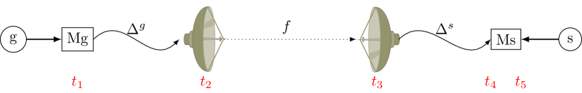
(a) Sequence of events

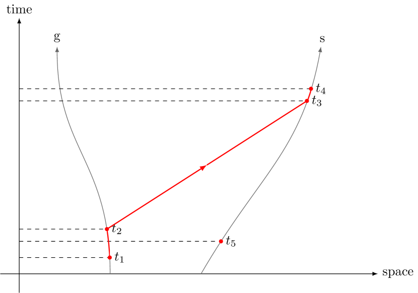
(b) Space-time diagram

Figure 3: Schematic representation of the one-way link.

Let’s consider a one-way link between a ground and a space clock represented respectively by superscripts $g$ and $s$. The sequence of events is illustrated on figure 3. At time coordinate $t_{1}$, clock $g$ displays time $\tau^{g}(t_{1})$ and modem Mg produces a code $C^{1}$. This code modulates a sinusoidal signal of frequency $f$ and is sent at coordinate time $t_{2}$ by antenna $g$. The time delay between the code production and its transmission by antenna $g$ is $\Delta^{g}=[T_{12}]^{g}$, expressed in local frame of clock $g$. Antenna $s$ receives signal $C^{1}$ at coordinate time $t_{3}$, and transmits it to modem Ms and clock $s$ which receives it at coordinate time $t_{4}$, with a delay $\Delta^{s}=[T_{34}]^{s}$, expressed in local frame of clock $s$.

The codes produced by the ground and the space clocks are the same, meaning that for the same proper time displayed by the clocks the same piece of code is produced. This is an unambiguous way to synchronize the signal to the proper time of the clocks. We implicitly define the coordinate time $t_{5}$ when clock $s$ displayed the same code $C^{1}$ as encoded in the received signal:

$$\tau^{s}(t_{5})=\tau^{g}(t_{1})\ .$$ (2)

The pseudo-time-of-flight $\Delta\tau^{s}$ (PToF, see section 2.2) given by the receiver $s$ is then defined as:

$$\Delta\tau^{s}(\tau^{s}(t_{4}))\equiv\tau^{s}(t_{5})-\tau^{s}(t_{4}).$$ (3)

The PToF is dated with proper time of clock $s$ when this clock receives code $C^{1}$ from antenna $s$. It can be interpreted as the difference between the proper time of production of code $C^{1}$ by clock $s$, and the proper time of reception of the same code $C^{1}$ sent by clock $g$, all expressed in proper time of clock $s$.

Then the desynchronization $\delta$ between clocks $g$ and $s$ is written in a hypersurface characterized by coordinate time $t=\mathrm{constant}$. From equations (2)-(3) it is straightforward to calculate the desynchronization at coordinate time $t_{4}$:

$$\delta(t_{4})\equiv\tau^{s}(t_{4})-\tau^{g}(t_{4})=-\Delta\tau^{s}\left(\tau^{s}(t_{4})\right)-\left[T_{23}+\left[\Delta^{g}+\Delta^{s}\right]^{t}\right]^{g}$$ (4)

Similar formulas can be obtained for the desynchronization at coordinate times $t_{1}$ and $t_{5}$. This expression has been obtained for the uplink, from ground to space. The desynchronization expression with downlink observables may be obtained by exchanging $g$ and $s$ in equation (4).

Let’s consider now a link which is composed of two one-way links, between a ground and a space clock represented respectively by subscript $g$ and $s$. The two sequences of events are illustrated on figure  4. The uplink (from ground to space) has a frequency $f_{1}$ and is represented by coordinate time sequence $(t_{1}^{0},t_{1},t_{2},t_{2}^{0},t_{7}^{0})$ (figure 4(a)). This link is defined with the relation:

$$\tau^{g}(t_{1}^{0})=\tau^{s}(t_{7}^{0}).$$ (5)

The downlink has a frequency $f_{2}$ and is represented by coordinate time sequence $(t_{3}^{0},t_{3},t_{4},t_{4}^{0},t_{8}^{0})$ (figure 3(b)). This link is defined with the relation:

$$\tau^{s}(t_{3}^{0})=\tau^{g}(t_{8}^{0}).$$ (6)

(a) Uplink sequence of events

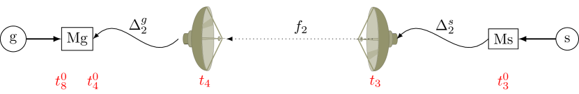
(b) Downlink sequence of events

(c) Space-time diagram

Figure 4: Schematic representation of the two-way link.

In the ACES/PHARAO mission we use the so-called $\Lambda$ configuration. This configuration minimizes the error coming from the uncertainty on ISS orbitography (in [17] it has been shown that in this configuration the requirement on ISS orbitography accuracy is around 10 m). The $\Lambda$ configuration is defined by $t_{2}=t_{3}$, i.e. code $C^{2}$ is sent at antenna $s$ when code $C^{1}$ is received at this antenna. This configuration is obtained by interpolating the observables in the data analysis software. Then it can be shown from equation (4) that the desynchronization between clocks $g$ and $s$ at coordinate time $t_{2}$ is:

$$\delta(t_{2})\equiv\tau^{s}(t_{2})-\tau^{g}(t_{2})=\frac{1}{2}\left(\Delta\tau_{\text{mo}}^{g}(t_{4}^{0})-\Delta\tau_{\text{mo}}^{s}(t_{2}^{0})+\left[T_{34}-T_{12}\right]^{g}\right).$$ (7)

where we introduced the corrected observables $\Delta\tau_{\text{mo}}^{g}$ and $\Delta\tau_{\text{mo}}^{s}$:

$$\begin{array}[]{lcl}\Delta\tau_{\text{mo}}^{g}(t_{4}^{0})&=&\Delta\tau^{g}\left(\tau^{g}(t_{4}^{0})\right)+\Delta^{g}_{2}+\Delta^{s}_{2}\\[7.22743pt] \Delta\tau_{\text{mo}}^{s}(t_{2}^{0})&=&\Delta\tau^{s}\left(\tau^{s}(t_{2}^{0})\right)+\Delta^{g}_{1}+\Delta^{s}_{1}.\end{array}$$ (8)

In equation (7) remains one transformation from coordinate to proper time. We know that $T_{12}\sim T_{34}\sim 1$ ms. During this time interval the gravitational potential and velocity of the ground station can be considered to be constant, leading to:

$$\left[T_{34}-T_{12}\right]^{g}=(1-\epsilon_{g}(t_{2}))\left(T_{34}-T_{12}\right),$$ (9)

where

$$\epsilon_{g}(t)=\dfrac{GM}{r_{g}(t)c^{2}}+\dfrac{v_{g}^{2}(t)}{2c^{2}},$$

$M$ is the Earth mass, $r_{g}(t)$ and $v_{g}(t)$ are the ICRS radial coordinate and the coordinate velocity of the ground clock at coordinate time $t$.

Orders of magnitude of these corrective terms are:

$$\dfrac{GM}{r_{g}c^{2}}T_{34} \sim 0.6\ \textrm{ps}$$

$$\dfrac{v_{g}^{2}}{2c^{2}}T_{34} \sim 0.002\ \textrm{ps}$$

The gravitational term is just at the limit of the required accuracy. The velocity term is well below, so we can neglect it. The final formula for desynchronisation is then:

$$\delta(t_{2})=\frac{1}{2}\left[\Delta\tau_{\text{mo}}^{g}(t_{4}^{0})-\Delta\tau_{\text{mo}}^{s}(t_{2}^{0})+\left(1-\frac{GM}{r_{g}(t_{2})c^{2}}\right)\left(T_{34}-T_{12}\right)\right].$$ (10)

In the $\Lambda$ configuration we suppose that $T_{23}=0$. However, this will never be exactly 0 and it will be known with an accuracy $\delta T_{23}$. This will add a supplementary delay $\delta(\tau^{s}-\tau^{g})$ to desynchronization (7):

$$\delta(\tau^{s}-\tau^{g})(t_{2})=\left(\epsilon_{g}(t_{2})-\epsilon_{s}(t_{2})\right)\delta T_{23}$$ (11)

Orders of magnitude are:

$$\dfrac{GM}{c^{2}}\left(\dfrac{1}{r_{g}}-\dfrac{1}{r_{s}}\right) \sim 2.8\times 10^{-11}$$

$$\dfrac{v_{g}^{2}-v_{s}^{2}}{2c^{2}} \sim -3.3\times 10^{-10}$$

With the required accuracy on the MWL, $|\delta(\tau^{s}-\tau^{g})|\lesssim 0.3$ ps, we deduce the following constraint on $\delta T_{23}$:

$$\delta T_{23}\lesssim 0.9\ \textrm{ms}.$$

This constraint is much less constraining than the one coming from orbitography, which is $\delta T_{23}\lesssim 1~{}\mu\textrm{s}$ (see [17]).

3.1.1 Atmospheric delays

The downlink is composed of two one-way links of frequencies $f_{2}$ and $f_{3}$, represented respectively by coordinate time sequence $(t_{3}^{0},t_{3},t_{4},t_{4}^{0},t_{8}^{0})$ and $(t_{5}^{0},t_{5},t_{6},t_{6}^{0},t_{9}^{0})$. These two links are affected by a ionospheric delay that depends on their respective frequencies, whereas the tropospheric delay does not depend on the link frequency. Dispersive troposphere effects can marginally reach the required uncertainties but are neglected at this stage. They can be taken into account using a global model [26]. We write:

$$T_{12} =\frac{R_{21}}{c}+\Delta^{\mathrm{iono}}_{12}(f_{1})+\Delta^{\mathrm{tropo}}_{12}+\Delta^{\mathrm{Shapiro}}_{21}$$ (12)

$$T_{34} =\frac{R_{34}}{c}+\Delta^{\mathrm{iono}}_{34}(f_{2})+\Delta^{\mathrm{tropo}}_{34}+\Delta^{\mathrm{Shapiro}}_{34}$$ (13)

$$T_{56} =\frac{R_{56}}{c}+\Delta^{\mathrm{iono}}_{56}(f_{3})+\Delta^{\mathrm{tropo}}_{56}+\Delta^{\mathrm{Shapiro}}_{56}$$ (14)

where $R_{ij}=|\vec{x}_{g}(t_{j})-\vec{x}_{s}(t_{i})|$ is the range, $\vec{x}_{s}$ and $\vec{x}_{g}$ are respectively position vectors of space and ground antennas, $r_{s}=|\vec{x}_{s}|$, $r_{g}=|\vec{x}_{g}|$ and:

$$\Delta^{\text{Shapiro}}_{ij}=\dfrac{2GM}{c^{3}}\ln\left(\dfrac{r_{s}(t_{i})+r_{g}(t_{j})+R_{ij}}{r_{s}(t_{i})+r_{g}(t_{j})-R_{ij}}\right)+\mathcal{O}(c^{-4})$$ (15)

Ionospheric and tropospheric delays are around or below 100 ns, whereas Shapiro delay (term in $c^{-3}$) is below 10 ps for the ACES/PHARAO mission (see [27] and A).

3.1.2 Tropospheric delay and range

By adding ground and space observables of links $f_{1}$ and $f_{2}$ we obtain:

$$\begin{array}[]{l}\Delta\tau^{s}(\tau^{s}(t_{2}^{0}))+\Delta\tau^{g}(\tau^{g}(t_{4}^{0}))+\Delta^{g}_{1}+\Delta^{g}_{2}\\[7.22743pt] +\left[\left[\Delta^{s}_{1}+\Delta^{s}_{2}\right]^{t}\right]^{g}=\left[T_{23}^{0}\right]^{s}-\left[T_{23}^{0}\right]^{g}-\left[T_{12}+T_{34}\right]^{g}\end{array}$$

As in the previous section, it can be shown that $\left[T_{23}^{0}\right]^{s}-\left[T_{23}^{0}\right]^{g}\simeq 0$ if $T_{23}^{0}$ is known with an accuracy $\delta T_{23}^{0}\lesssim 0.9$ ms. We neglect the coordinate to proper time transformations for delays $\Delta^{s}$ and obtain

$$T_{12}+T_{34}=-\left(1+\dfrac{GM}{r_{g}(t_{2})c^{2}}\right)\left(\Delta\tau_{\text{mo}}^{s}(t_{2}^{0})+\Delta\tau_{\text{mo}}^{g}(t_{4}^{0})\right),$$

Then, from equations (12)-(13) we obtain:

$$\dfrac{R_{21}+R_{34}}{c} = -\left(1+\dfrac{GM}{r_{g}(t_{2})c^{2}}\right)\left(\Delta\tau_{\text{mo}}^{s}(t_{2}^{0})+\Delta\tau_{\text{mo}}^{g}(t_{4}^{0})\right)$$

$$-\left(\Delta^{\text{iono}}_{12}(f_{1})+\Delta^{\text{iono}}_{34}(f_{2})+\Delta^{\text{tropo}}_{12}+\Delta^{\text{tropo}}_{34}\right)$$

$$-\left(\Delta^{\text{Shap}}_{21}+\Delta^{\text{Shap}}_{34}\right)$$

where Shapiro delay is added for completeness; practically it should be negligible compared to the error of the tropospheric model. The ionospheric delays are obtained from the two downlink observables (see A), but as can be seen from equation (3.1.2) the range and tropospheric delays are degenerate. Range can be calculated with a model for tropospheric delay, and tropospheric delay can be calculated from an estimation of range.

3.2 From raw data to Pseudo-Time of Flight

Initial algorithms development have been made assuming that the microwave link data would be similar to pseudo-time of flight (PToF), as issued by GNSS receivers. In the course of hardware development, it appeared that a rather different approach would be used by the manufacturer, based on local signal beatnotes and counter measurements. In a first and independent “preprocessing” step our software transforms those raw measurements into PToF that are then used in further processing.

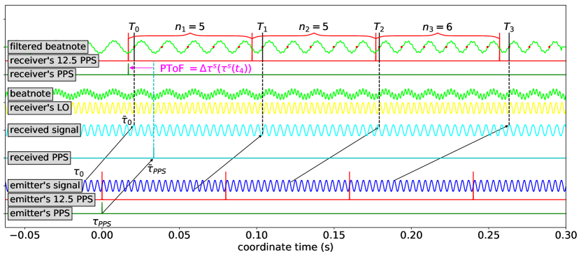
Figure 5: Schematic representation of the measurements provided by the hardware: both emitter’s and receiver’s signals are represented against the coordinate time scale. 1 PPS (dark green) and 12.5 PPS (red) pulses for the emitter and the receiver are represented. The emitter’s carrier is represented by the blue sine at the bottom. Propagation delays are represented by black arrows. Incoming PPS and carrier are affected by this (variable) delay and appear in cyan. Local oscillator (yellow) is mixed with incoming carrier to give the green beatnote, which is then filtered. Red dots on the filtered beatnote indicate zero crossings on ascending edge. $n_{m}$ is the number of red dots between two 12.5 PPS pulses. $T_{m-1}$ is the proper time of the first red dot within the same interval. Signal frequency is much lower than in reality. Doppler effect is strongly magnified in order to show the variation of $n_{m}$. Finally, the observable we want to determine (PToF) is represented as a purple arrow.

Detailed description of the algorithms is out-of-scope of this article, but an overview may be found in figure 5. It can roughly be read as a chronogram, with several signals being superposed on it :

• The 3 bottom lines represent a sinusoidal signal, a 1 PPS and a 12.5 PPS that delimitates 80 ms intervals. These 3 signals are generated at the emitter’s level, and are locked to the local clock signal (they are the best realization of the clock proper time): for simplicity, we represented the first PPS of the emitter at the origin of coordinate time.

• The “received signal” corresponds to the emitter’s signal as received by the remote station: the black arrows represent the propagation delay for several events, which changes throughout the pass, and produces a classical Doppler effect.

• The upper part of the graph represents what happens at the receiver’s level : 1 and 12.5 local PPS are generated, together with a local sine signal (“receiver’s Local Oscillator”). Mixing the received signal and the local oscillator generates a beatnote, which is filtered through a low-pass filter.

• Then the measurement takes place : for each 80 ms period, the device counts the number of ascending zero-crossings of the filtered beatnote, $n_{m}$, and the date of the first zero-crossing, $T_{m}$. $n_{m}$ variations are mostly due to Doppler effect on received signal. Note that measurement occurs at the first zero crossing, so it is not natively aligned with 80 ms interval.

From $(T_{m},n_{m})$ couples, we have to recover the time difference represented in purple: $\Delta\tau^{s}(\tau^{s}(t_{4}))$, which is a PToF : for a given proper time, the main contributions to this value are the desynchronisation between the two clocks, minus the propagation delay.

3.3 Code and carrier ambiguities

As explained in the previous section, we get from the receiver modem (space and ground) three kinds of files: pulse (PPS arrival times), code ($T_{m}$, $n_{m}$) and carrier ($T_{m}$, $n_{m}$). Code is in principle unambiguous (within the code’s length) and chip counters are implemented to ensure that. However, for historical and technical reasons, we have chosen to not use the chip counters, but instead treat the code the same way as the carrier i.e. to work with a code ambiguity corresponding to a 100 MHz cycle (one chip length), and, as for the carrier, lift that ambiguity using a coarser measurement, namely the pulse data. From it, we deduce coarse times of emission and reception of the signal, roughly every 1 second, such that we can directly calculate the PToF. However we are limited in accuracy by the quantization of the time counter ($\approx$ 10 ns) that registers the PPS arrival times and the $T_{m}$ value, well above the targeted accuracy. This pulse observable will be used to remove the ambiguity on the code, then on the carrier observables. In this section we explain one method allowing to find the code and carrier ambiguities.

Let’s consider the one-way link described in section 3.1. The signal is sent at $\tau\equiv\tau^{g}(t_{1})$ in the local time of the emitter, and received at $\bar{\tau}\equiv\tau^{s}(t_{4})$ in the local time of the receiver, neglecting here, for simplicity, instrumental and ionospheric delays. Let $\Phi_{\text{L.O.}}$ be the phase of the receiver local oscillator, while $\Phi_{\text{Rx}}$ and $\Phi_{\text{Tx}}$ are respectively the phase of the received and emitted signal (see figure 5). Then:

$$\Phi_{\text{L.O.}}(\bar{\tau})=\omega_{\text{L.O.}}\bar{\tau}+\phi_{\text{L.O.}}^{0}$$ (17)

$$\Phi_{\text{Rx}}(\bar{\tau})=\Phi_{\text{Tx}}(\tau)=\omega_{\text{Tx}}\tau+\phi_{\text{Tx}}^{0}$$ (18)

where the origin of the phases $\phi_{\text{L.O.}}^{0}$ and $\phi_{\text{Tx}}^{0}$ are unknown. There is a known relation between the local oscillator phase $\Phi_{\text{L.O.}}$, the phase of the received signal $\Phi_{\text{Rx}}$ and the beatnote phase $\Phi_{\text{b}}$. The angular frequency of the code is higher than the angular frequency of the code local oscillator, such that $\Phi_{\text{b}}=+(\Phi_{\text{L.O.}}-\Phi_{\text{Rx}})$ for the code signal, while the angular frequency of the carrier is lower than the angular frequency of the carrier local oscillator, such that $\Phi_{\text{b}}=-(\Phi_{\text{L.O.}}-\Phi_{\text{Rx}})$ for the carrier signal. Using equations (17)-(18), we deduce:

$$\omega_{\text{Tx}}\Delta\tau(\bar{\tau})=(\omega_{\text{b}_{0}}\bar{\tau}-\Phi_{\text{b}}(\bar{\tau}))+\phi_{\text{L.O.}}^{0}-\phi_{\text{Tx}}^{0}$$ (19)

$$\omega_{\text{L.O.}}\Delta\tau(\bar{\tau})=(\omega_{\text{b}_{0}}\tau-\Phi_{\text{b}}(\bar{\tau}))+\phi_{\text{L.O.}}^{0}-\phi_{\text{Tx}}^{0}$$ (20)

where $\Delta\tau(\bar{\tau})=\tau-\bar{\tau}$ is the PToF, and $\omega_{\text{b}_{0}}$ is the “zero Doppler” beatnote angular frequency, i.e. $\omega_{\text{b}_{0}}=\pm(\omega_{\text{L.O.}}-\omega_{\text{Tx}})$ ($+$ sign for code and $-$ sign for carrier). Typical values of $\omega_{\text{b}_{0}}/(2\pi)$ are 195 kHz and 729 kHz for the code and carrier respectively.

The ambiguity in the calculation of the PToF $\Delta\tau$ comes from the fact that $(\phi_{\text{L.O.}}^{0}-\phi_{\text{Tx}}^{0})$ is unknown. Fortunately, the code and pulse signals are designed such that $(\phi_{\text{L.O.}}^{0}-\phi_{\text{Tx}}^{0})/(2\pi)$ is an integer. Moreover, the beatnote phase $\Phi_{\text{b}}$ can be interpolated from the modem code observables $(T_{m},n_{m})$ (see previous section) up to a multiple of $(2\pi)$, and we call $\tilde{\Phi}_{\text{b}}$ the interpolated beatnote. Therefore one has:

$$\phi_{\text{L.O.}}^{0}-\phi_{\text{Tx}}^{0}-\Phi_{\text{b}}(\bar{\tau})=2\pi k-\tilde{\Phi}_{\text{b}}(\bar{\tau})$$ (21)

where $k$ is an unknown integer, and we deduce from equations (19)-(20) for the pulse and the code:

$$f_{\text{Tx}}^{\text{co}}\Delta\tau(\bar{\tau})=f_{\text{b}_{0}}^{\text{co}}\bar{\tau}+k-\frac{\tilde{\Phi}_{\text{b}}^{\text{co}}(\bar{\tau})}{2\pi}$$ (22)

$$f_{\text{L.O.}}^{\text{co}}\Delta\tau(\bar{\tau})=f_{\text{b}_{0}}^{\text{co}}\tau+k-\frac{\tilde{\Phi}_{\text{b}}^{\text{co}}(\bar{\tau})}{2\pi}$$ (23)

Relation (23) can be used with the pulse observables to find $k$, because we know both $\tau$ and $\bar{\tau}$ for the pulse, and the 10 ns accuracy of the pulse PToF $\Delta\tau$ can be shown to be sufficient after a little averaging ($k$ remains constant during continuous lock of the signal e.g. during a pass). Using the value of $k$ found with the pulse observable we then remove the ambiguity on the code observable using relation (22).

For the carrier signal the quantity $(\phi_{\text{L.O.}}^{0}-\phi_{\text{Tx}}^{0})/(2\pi)$ is not an integer anymore. Therefore relation (19) can be written for the carrier observable:

$$f_{\text{Tx}}^{\text{ca}}\Delta\tau(\bar{\tau})=-f_{\text{b}_{0}}^{\text{ca}}\bar{\tau}+j+\frac{\tilde{\Phi}_{\text{b}}^{\text{ca}}(\bar{\tau})}{2\pi}+\frac{\phi^{\text{ca}}_{0}}{2\pi}$$ (24)

where $j$ is an unknown integer and $0\leq\phi^{\text{ca}}_{0}<2\pi$ is an unknown phase origin. This relation can be used to find both $j$ and $\phi^{\text{ca}}_{0}$: one has to interpolate the absolute code series found earlier using relation (22), with an error of the order of 20 ps. Therefore we can find $j$ for each pass, but the determination of $\phi^{\text{ca}}_{0}$ will be limited by the accuracy of the absolute code series. Then it is not possible to find a better determination of the absolute PToF for one individual pass using the carrier. However, $\phi^{\text{ca}}_{0}$ is common to all passes; using several passes it is possible to average the error done on its determination up to an error $\sim 20$ ps$/\sqrt{N}$, where $N$ is the number of passes. It would then take around 1600 passes to attain the targeted carrier accuracy which is of the order of 0.5 ps. Fortunately, for most science objectives, we do not need this accuracy on the absolute PToF but only on their differences, for which the term $\phi^{\text{ca}}_{0}$ cancels out.

4 Data analysis and simulation

4.1 Implementation of the simulation

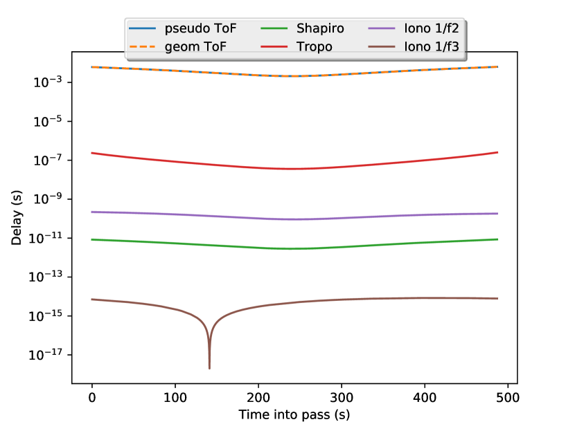
Figure 6: Contribution of atmospheric and Shapiro delays in the simulated time-of-flight of the $f_{1}$ signal for carrier observables (absolute values). Pseudo ToF is the sum of all other components and is dominated by geometrical time of flight (curves are superposed here). Ionospheric delay is split between its $1/f^{2}$ and $1/f^{3}$ terms, the latter being negligeable for Ku-band data but much larger for S-band.

In order to test the data analysis software, a simulation of the mission observables has been written in Matlab ($\simeq 4000$ lines). It is as independent as possible from the data analysis software: different coding language, algorithms, etc…It takes as input orbitography of the ISS and terrestrial coordinates of a Ground Station (GS). The ISS trajectory is either simulated (Kepler orbit) or a real trajectory read from an sp3 file (https://igscb.jpl.nasa.gov/igscb/data/format/sp3c.txt). In the case of a real trajectory for the ISS and for the GS, the coordinate transformations from terrestrial to celestial frame are computed with the SOFA routines (see section 2.3). For a given number of days the simulation then calculates the times of passes for the GS corresponding to a given elevation cutoff of the ISS.

From the trajectories and a model of the geo-potential the simulation calculates the relation between proper times given by ISS and GS clocks and the coordinate time. In an effort to keep numerical accuracy below the targeted accuracy (timing error below 0.3 ps throughout one pass and between passes) local timescales for all passes, linked to a global timescale, have been introduced. The time-of-flight (ToF) of the signal has several contributions: geometrical, ionospheric, tropospheric and Shapiro (see equations (12)-(14)). The geometrical ToF is calculated numerically by solving a two-point boundary value problem by means of the shooting method [28]. The ionospheric delay depends on the electron density profile in the atmosphere (see equations (28)-(29)) and on the magnetic field. The STEC $S$ can be chosen as constant or integrated from a Chapman layer model [29] for a more realistic delay. The magnetic field is a simple dipole model in the simulation, while we have chosen a more sophisticated model for the data analysis in order to check the effect of a mismodeling of the magnetic field. We can see no effect above the targeted noise due to this difference of model. Finally, we use a Saastamoinen model in order to calculate the tropospheric delay [30].

The Saastamoinen model is not really reliable at low elevation of ISS and the dispersive part of troposphere has not been taken into account. Indeed, the main scientific product of the ACES experiment is desynchronization, which does not require a high precision tropospheric model to be calculated. The only constraint is to be able to perform the $\Lambda$-configuration interpolation, which requires an accuracy better than 30 m on the range. To this end the Saastamoinen model is sufficient. However, in order to obtain the best accuracy for the range as a secondary scientific product, it is necessary to disentangle the geometric ToF from the tropospheric ToF (see section 3.1.2). Independent studies have been performed [26, 31] in order to study the best available model for the tropospheric delay, including the dispersive part.

In figure 6 we have plotted different contributions included in the ToF of signal $f_{1}\simeq 13.5$ GHz. Minimum elevation of ISS is taken as 10 degrees, and atmospheric parameters are temperature $T=298$ K, pressure $p=1$ bar and water vapor pressure $e=0.5$ bar. A sinusoidal variation is added to atmospheric parameters, with a period of 24 hours, and a Chapman layer model is used to calculate the STEC. Tropospheric delay is dominant in the ToF, with a value of several 10 ns. Ionosphere is dispersive such that ionospheric delay can be separated in two contributions: an effect that scales with $1/f^{2}$ and one that scales with $1/f^{3}$ (see equations (28)-(29)). The second order contribution is around 1 ns and the third contribution around 0.1 ps, below mission accuracy. However these effects are much larger for the $f_{3}=2.25$ GHz signal: around 40 ns for second order term and 20 ps for third order term. Then third order terms cannot be ignored. The Shapiro delay of several ps is slightly over the required accuracy, but, as already mentioned, cancels in the two-way combination and is negligible with respect to tropospheric model uncertainties in one-way or range measurements.

Finally, pseudo-time-of-flight (PToF) are calculated from the ToF and the coordinate to proper time transformation for the GS and the ISS. Then PToF are used to generate the modem observables $(T_{m},n_{m})$ (see section 3.2). This procedure is repeated six times (for the three signals, and for the code and carrier) in order to produce the simulated observables files which are in the same format as the operational files. Some features can be added optionally such as signal multipath, non-null initial desynchronization of the clocks, clock noise and orbitography errors. The simulation produces all blue boxes (except calibration data) and red boxes shown in figure 7 in order to test the data analysis software.

4.2 Data analysis software

Software has been developped in Python3 (https://www.python.org/), relying on NumPy and SciPy [32, 33] for the (moderately) heavy numerical calculations, matplotlib [34] being used for data graphing. This allows satisfactory performance while keeping good readability and maintainability. The module has been encapsulated as a Python package for easier deployment and version management on production servers.

From the onset, this software has been designed as a pipeline, intended to run as automatically as possible. However it is also possible to process individual data, while picking which modules should be run (e.g. troposphere delay, ionosphere delay, etc…).

The goal is to transform raw data (the output of ground terminals and flight segment) into scientific outputs, namely : the desynchronisation between a given ground terminal clock and the flight segment, as well as some byproducts (Total Electron Content, and a mix of range and tropospheric delays). To achieve this, additional inputs are needed : position of the ISS and the ground station during the pass, atmospheric parameters, and various calibration coefficients (see figure  7).

Figure 7: Global flow chart for the MWL data analysis software.

Input categories include :

• Calibration data : all instrumental effects have to be removed before analyzing the data. This is done by applying calibration coefficients and/or adding a calibration delay to the raw data, following procedures provided by the manufacturer.

• On-board and ground station raw data : for a given pass, data collected by the on-board terminal and the corresponding ground terminal are gathered from the archive and fed to the software. Data is sampled at 12.5 Hz, independently for uplink and downlink (i.e. there can be up to 40 ms delay between an uplink data point and the closest corresponding downlink data point).

• Orbitography : By using a two-way time transfer, at first order the one-way propagation time of the signal cancels out, but the variation of this delay between forth and back paths does not : this effect may shift the desynchronisation measurement (up to 10 ns in the least favourable configurations), so it should be mitigated with a priori knowledge of the respective positions of the terminals, e.g. orbitography of the ISS and position of the ground terminal. Naming ground station position “Ground orbitography” stresses the symmetry between both stations : in a non-rotating frame, ground stations also are in motion during the signal’s propagation.

• Atmospheric parameters are used for first order estimation of the tropospheric delay

Scientific outputs include (see section 3):

• The clock desynchronization between ground and space, obtained from the difference between uplink and downlink Ku band measurements. This measures, for a given coordinate time $t$, the difference between the ground clock’s proper time and the space clock’s proper time.

• The Total Electron Content, derived from the difference between Ku and S band downlink measurements. This is a by-product of the ionospheric delay determination, which is necessary to correct the desynchronisation product.

• A mix of range and tropospheric delays obtained from the sum of uplink and downlink Ku band measurements. Modelling one of those two effects allows to derive the remaining one.

4.3 Validating the software with simulated data

Data analysis preparation has begun long before any “real” data was available. Moreover, the flexibility of our simulation software allows us to investigate cases that cannot be emulated on the hardware. Finally, the ability to generate two datasets with only one parameter being changed, all others being kept identical, is a very useful tool to validate the individual modules of our codes.

The rather strict separation we maintained between data analysis and simulation code development allowed us to highlight bugs in both codes efficiently. Although we cannot rule out that a common misunderstanding of hardware specifications leads to mutually cancelling bugs in simulation and data analysis, we are confident that most of them have been solved this way. Definite proof will, of course, only be available once actual hardware data will be fed into the data analysis software.

For each pass, a set of simulated data is generated, along with a corresponding set of theoretical data. The former contains what we suppose will come out of the Ground Segment, i.e. phase counter values as decommuted from telemetry. The latter contains the corresponding theroretical values, which is a list of what has been calculated at different steps in the simulation software : scientific products but also intermediary values (e.g. tropospheric delay, ionospheric delay, etc…) are thus directly comparable to the corresponding values as calculated by the data analysis software.

We cannot expect full recovery of those values : the fact that data is only collected through counter values introduces an uncertainty on all of them. We assume that a specific calculation is validated when, for one pass, the offset and scatter of all data points within this pass are compatible with the dispersion expected from this truncation.

For example, we know from the MWL measurement principle [35] that the main counter frequency runs at 100.1953125 MHz. This means that any timetag derived from this counter is truncated at $\simeq$ 10 ns resolution. This converts into a 20 ps resolution on code pseudo-range (taking advantage of the fact that we measure the phase of a beatnote: 10 ns $\times f_{\text{b}_{0}}^{\text{co}}/f^{\text{co}}\approx$ 10 ns $\times$ 195 kHz/100 MHz $\approx$ 20 ps). When plotting the residuals (calculated - expected value) for each point of the pass, we expect a random dispersion with a width of 20 ps. Moreover, code data should be unambiguous, so we expect the theoretical value to be within this spread (i.e. the 20 ps range of residuals contains 0). So, for the case of code pseudo-range, our validation criteria should be: peak-to-peak residuals $\leq$ 20 ps, residuals mean offset between -10 ps and +10 ps. Similarly for carrier measurements we expect a resolution of about 0.5 ps ($\approx$ 10 ns $\times f_{\text{b}_{0}}^{\text{ca}}/f^{\text{ca}}\approx$ 10 ns $\times$ 729 kHz/14 GHz), with an overall offset that is no better than 20 ps/sqrt(N) for N passes, but should be within 0.5 ps between passes (see section 3.3).

A less quantitative (and less absolute) criterion is the absence of notable signature in the residuals : most of the time we expect the spread to be uniform across the pass, and any visible pattern should be investigated as a possible consequence of implementation problems.

Figure 8 shows the typical results we expect to get when processing a single pass and compare the result to input values. Each point on the bottom graph is a difference between the simulated (“theoretical”) value, and the value we obtain at the end of data anlysis. Here we only show results for the desynchronisation, but similar graphs can be drawn for any intermediate result which is calculated for each data point (e.g. TEC, ionospheric delay, etc…). Code and carrier observables are obtained from distinct datasets, with similar algorithms : as they measure the same physical quantities we use the former to determine the latter’s offset, although an overall residual offset will remain in the carrier data (see section 3.3).

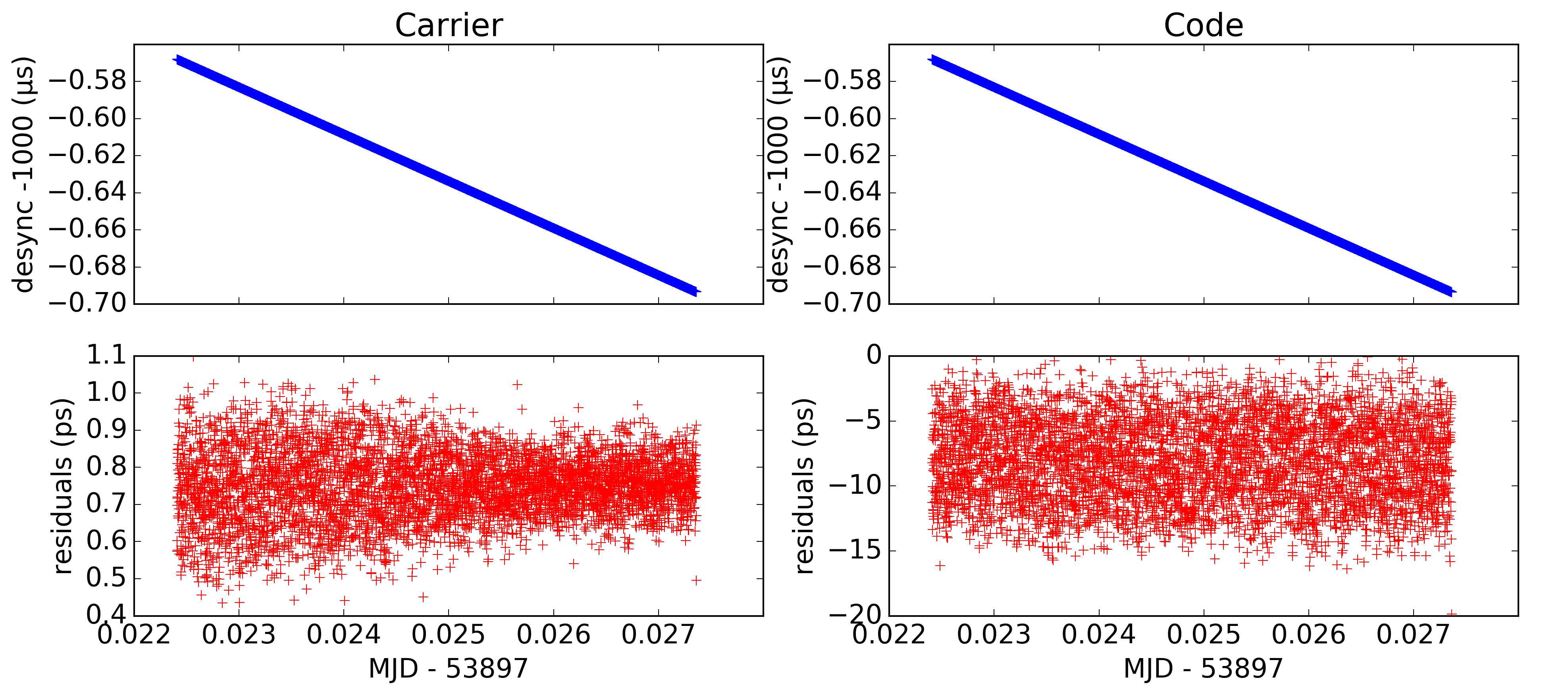
Figure 8: Typical pass data. Top : input values for desynchronisation. Bottom : difference between input values and processed data. Noise is linked to the counter’s resolution and represent the noise floor of the MWL.

It should be noted that, although the desyncronisation value (top line) spans more than 10 ns during the pass (which is expected, due to gravity potential and velocity difference between ground and space), we recover its value with a peak to peak spread <1 ps for carrier and <20 ps for code.

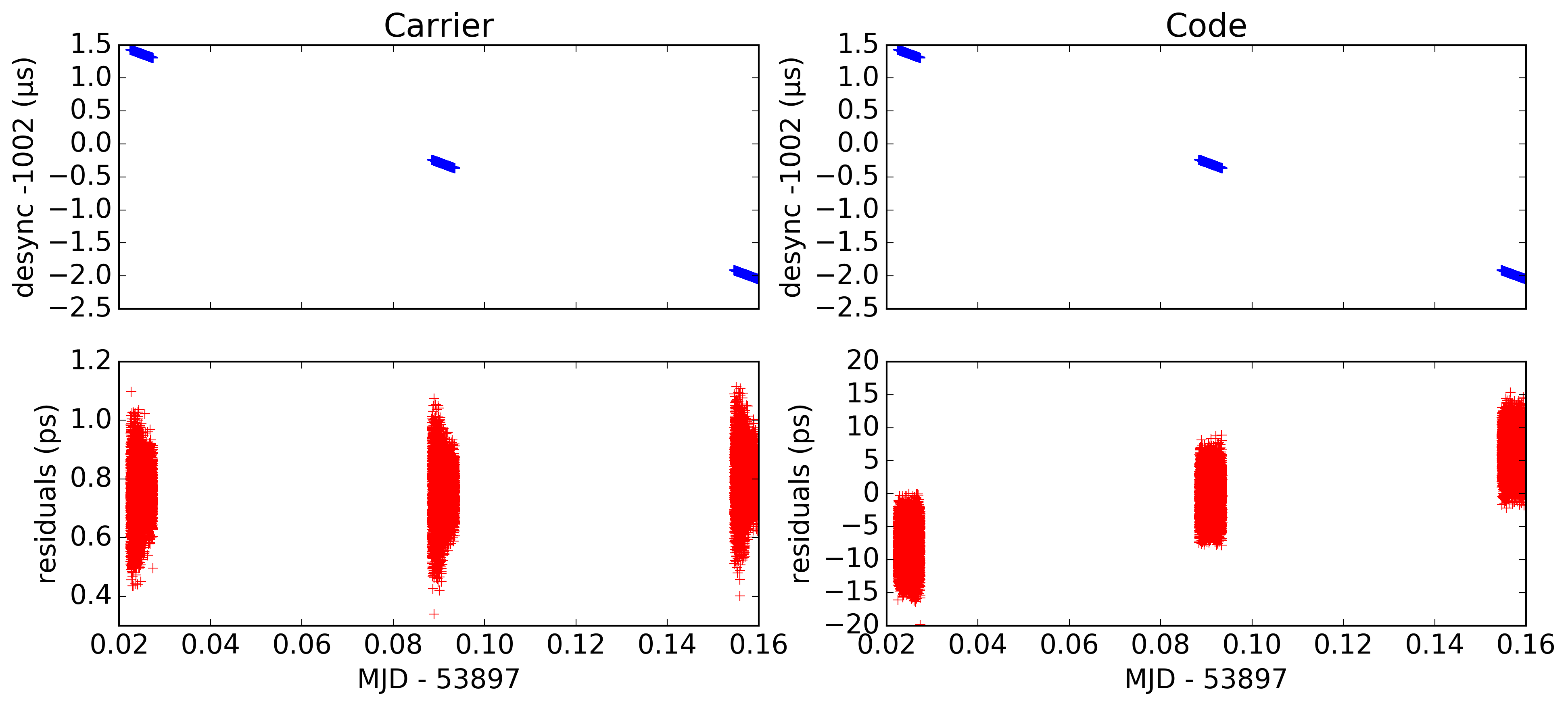
Figure 9: Similar to fig 8 but with a larger time span, showing several successive ISS visiblility periods. As expected, code residuals show mean values in the -10/+10 ps range. Carrier residuals stay close to their initial value (which will be unknown in flight).

One of the key achievements needed to fulfill the ACES mission goals is the ability to link results from one pass to the next : we will then be able to track time differences on periods of time much longer than one pass. As code data is unambiguous this is directly the case, albeit with a poor stability. Carrier data is more challenging to deal with, but will bring the required stability.

Based on our understanding of the measurement method [35], we have implemented a processing algorithm that recovers the carrier phase difference, up to an unknown offset which is set at device switch on (see section 3.3). In other words, as long as both the emitter and the receivers remain switched on, our analysis software is able to recover time differences from the counter values with an overall offset, but a peak to peak spread better than 1 ps at 80 ms. Figure 9 illustrates this capability on 3 successive passes. Here the only source of uncertainty is the truncation due to the counters running at 100 MHz : we expect performance to be worse in operation because of additional perturbations and noise sources.

5 An experiment : impact of ISS orbitography errors

An immediate application of our simulation and analysis software is to check if previous assumptions on input uncertainty impact are correct. We first had a look at the impact of ISS orbitography uncertainty, which has already been modeled analytically in [17].

5.1 Method

The basic principle of our test is to use different orbitography data as input for the simulation and for the data analysis. The simulation’s orbitography is then supposed to be the “real” one, i.e. the one we would get if we had perfect knowledge of the ISS position. Then we fetch a slightly different data as input to the analysis software : this represents the “measured” orbitography, i.e. the one that will be available when we perform the analysis.

Modelling the uncertainty on ISS position is not straightforward, as already noted in [17]. Our approach here has been instead to use existing data to estimate the position error for a given period : we took advantage of a measurement campaign [36] when both standard Space Integrated GPS/INS (SIGI) data and more precise GNSS positioning data (from ASN-M russian receiver) were available. Then, if we compare two positions given for the same date, most of the error comes from the SIGI uncertainty [37] so the difference between the two vectors is a good estimator of the overall measurement error we would have made, if we had only the SIGI data.

Note that the SIGI uncertainty we assume (see figure 10) is likely to be a pessimistic estimate of the ACES orbitography error as the ACES payload has its own GNSS receiver which should significantly improve orbit restitution.

Furthermore, we wanted to be able to modulate this error (i.e. emulate a stronger or weaker uncertainty with respect to the real value). We therefore wrote a tool that

• Calculates a positional error from (SIGI - GNSS) data

• Projects the resulting vector in a relevant reference frame (RTN, see below)

• Multiplies each R, T, N component of that vector by a given coefficient. Below we use the same coefficient $k_{err}$ for all three axes.

• Adds the resulting vector to the initial orbitography, providing the “erroneous” orbitography for the analysis software.

5.2 Introduced orbitography errors

We chose a period starting at MJD 53896 and ending at 53908, as altitude and velocity data revealed no obvious event (e.g. altitude boost) during this period. Resulting error is shown on figure 10.

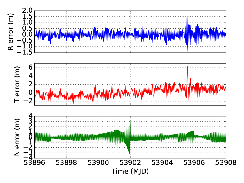
Figure 10: Difference between regular SIGI and GNSS ISS orbitography during a boost-free period.

All three orbit error components display a strong periodic component at the orbital frequency as one might expect. The overall peak to peak error is about 8 m in T and N and somewhat less (about 3 m) in R.

5.3 Effect on desynchronization

As a first approach we applied several levels of ISS position uncertainties, using the same coefficient on R, T and N, on 57 consecutive passes (spanning 10 days of data). We examined the effect of such uncertainty on the desynchronisation residuals, and compared it to an ideal case where ISS position is known exactly. For each coefficient ($k_{err}=0/1/10/100$, corresponding roughly to 0 m, 10 m, 100 m and 1 km peak-to-peak error), we calculated carrier desynchronisation residuals for all 57 passes, as illustrated on the bottom left of figure 8. Then we calculated the corresponding TDEV for each pass. Figure 11 represents the Time Deviations (TDEV) calculated for each value of $k_{err}$ together with the MWL specifications. A TDEV is calculated for each one of the 57 passes, but only the mean value and the 80 % interval (shaded regions) are shown.

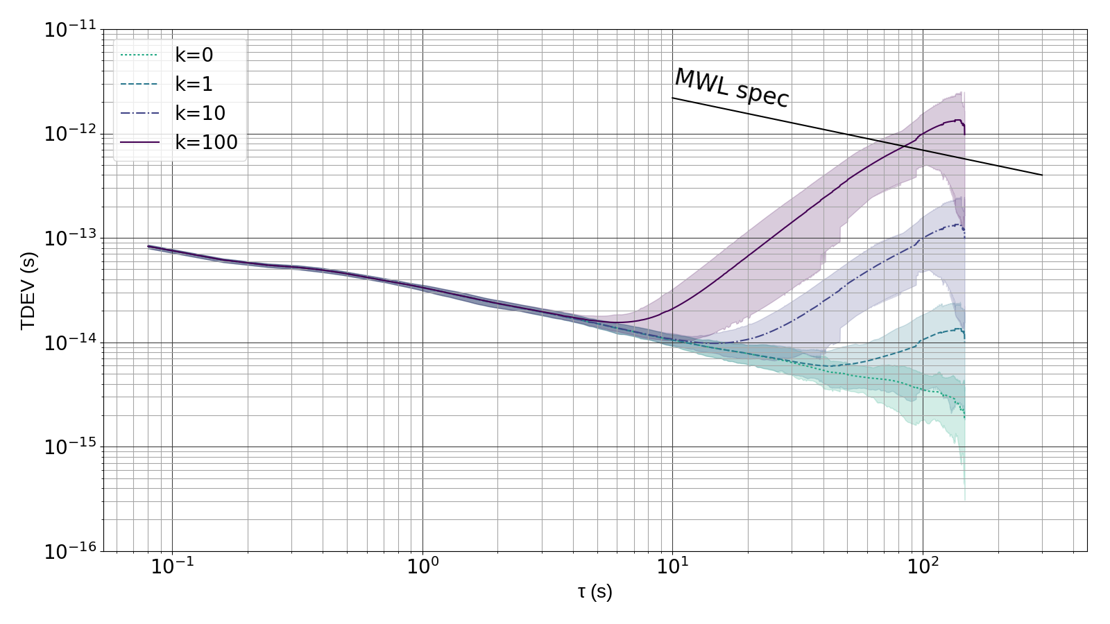
Figure 11: Effect of various uncertainty amplitude on desynchronisation residuals. Solid and dotted curves represent the mean value of TDEV over all 57 passes as a function of time interval $\tau$, for each value of $k$. The shaded enveloppes contain 80% of the values around this mean value to illustrate the spread. “MWL spec” represents the specification for the Micro Wave Link.

5.4 Discussion

The ideal case (coefficient = 0) shows that the counter quantization, which is the only perturbation here, introduces an error which is more than 2 orders of magnitude better than the specification. As the coefficient grows, it can be seen that time deviation grows accordingly towards large $\tau$ ($\simeq$ 0.5 pass length) while short term statistics is almost not affected. With an uncertainty 100 times worse than expected, the TDEV begins to be out of specifications.

This leaves a comfortable margin, especially when recalling that the actual orbitography errors should be smaller than the estimates used here because of the additional GNSS receiver on the ACES platform. Note however, that other perturbations will likely degrade the performance (imperfect instrumental calibrations, uncertainty on atmospheric delays, internal delay variations, etc…).

Our results confirm the analytical estimates of [17] for the orbitography requirements ($\approx 1$ km) coming from the specifications on the time transfer performance. However, as shown in [17] the requirements coming from the specifications on the integrated effect of the gravitational redshift and second order Doppler shift are much more stringent ($\approx 10$ m). A study by numerical simulation of those effects and of their influence on the science objectives is under way and will be published in a separate paper.

6 Conclusion

In this article we have explained our current understanding of the necessary steps needed to analyze the data that will be available once ACES is operational. We also exposed some of the underlying principles and algorithms that will allow us to perform such tasks, as well as the validation tools that are being used for development.

We demonstrated our ability to process typical batches of data ($\simeq$ 10 days), which is an important milestone in our effort to run a Data Analysis Center that will have to process such batches routinely during ACES operation.

As an example of application of these software tools we have used them to demonstrate that typical ISS orbitography errors ($\sim 10$ m) affect the MWL well below its performance specifications, and thus have negligible impact on the science objectives that depend on that performance.

Final software development will occur during the remaining phases prior to launch: as soon as the definitive hardware becomes available and data schemes freeze, we will need to fine-tune our algorithms and adapt our flow to possible deviations with respect to the present situation or assumptions.

Appendix A Ionospheric delays and computation of STEC

This section gives additional details on ionospheric delays calculation and orders of magnitude. In order to deduce ionospheric delays, we combine the two ground observables to be free of tropospheric delays. We obtain:

$$\begin{array}[]{l}\Delta\tau^{g}(\tau^{g}(t^{6}_{0}))-\Delta\tau^{g}(\tau^{g}(t^{4}_{0}))=\left[T_{34}-T_{56}\right]^{s}\\ +\left[T_{46}^{0}\right]^{s}-\left[T_{46}^{0}\right]^{g}+\Delta^{s}_{2}-\Delta^{s}_{3}+\left[\left[\Delta^{g}_{2}-\Delta^{g}_{3}\right]^{t}\right]^{s}\end{array}$$ (25)

Here we impose that $T_{46}^{0}=0$, i.e. both $f_{2}$ and $f_{3}$ measurements are done at the ground station at the same local time. However, this will never be exactly zero, there will be a remaining $\delta T_{46}^{0}$ introducing a timing error $\delta T\simeq\left(\epsilon_{s}(t_{4}^{0})-\epsilon_{g}(t_{4}^{0})\right)\delta T_{46}^{0}$. With a required accuracy $\delta T\lesssim 0.3$ ps, we obtain the following constraint:

$$\delta T_{46}^{0}\lesssim 0.9\ \textrm{ms}.$$

We expect that $|T_{34}-T_{56}|\lesssim 100$ ns (see [27]); therefore we can neglect the coordinate to proper time transformation in equation (25). We can also neglect this transformation for the delays. Then equation (25) is equivalent to:

$$\Delta\tau_{\text{mo}}^{g}(t_{6}^{0})-\Delta\tau_{\text{mo}}^{g}(t_{4}^{0})=T_{34}-T_{56}$$ (26)

From equations (13), (14) and (26) we obtain:

$$\Delta^{\text{iono}}_{56}(f_{3})-\Delta^{\text{iono}}_{34}(f_{2})=\Delta\tau_{\text{mo}}^{g}(t_{4}^{0})-\Delta\tau_{\text{mo}}^{g}(t_{6}^{0})+\dfrac{R_{34}-R_{56}}{c}$$ (27)

where we neglected the difference of the Shapiro delays between the two downlinks, which can be shown to be completely negligible.

Now we can calculate $S$ the Slant Total Electron Content (STEC). The ionospheric delay affects oppositely code (co) and carrier (ca) and may be approximated as follows (with S.I. units):

$$\Delta_{\text{co}}^{\text{iono}}(f) =\frac{40.308}{cf^{2}}S+\frac{7527}{f^{3}}\int N_{e}\left(\vec{B}\cdot\vec{k}\right)\textrm{d}L$$ (28)

$$\Delta_{\text{ca}}^{\text{iono}}(f) =-\frac{40.308}{cf^{2}}S-\frac{7527}{2f^{3}}\int N_{e}\left(\vec{B}\cdot\vec{k}\right)\textrm{d}L$$ (29)

where $N_{e}$ is the local electron density along the path, STEC $S=\int N_{e}\textrm{d}L$, $\vec{B}$ is the Earth’s magnetic field and $\vec{k}$ the unit vector along the direction of signal propagation. It has been shown that higher order frequencies effect can be neglected for the determination of desynchronization [27].

We suppose that for a triplet of observables

$$\{\Delta\tau^{s}(\tau^{s}(t_{2}^{0})),\Delta\tau^{g}(\tau^{g}(t_{4}^{0})),\Delta\tau^{g}(\tau^{g}(t_{6}^{0}))\}$$

the direction of signal propagation and of the magnetic field along the line of sight do not change, and $|\vec{B}|\simeq B_{0}$. Then:

$$\Delta_{\text{co}}^{\text{iono}}(f) =\frac{40.308}{cf^{2}}S\left(1+\frac{7527c}{40.308f}B_{0}\cos\theta_{0}\right)$$ (30)

$$\Delta_{\text{ca}}^{\text{iono}}(f) =-\frac{40.308}{cf^{2}}S\left(1+\frac{7527c}{80.616f}B_{0}\cos\theta_{0}\right),$$ (31)

where $\theta_{0}$ is the angle between $\vec{B}$ and the direction of propagation of signal $f_{2}$ and $f_{3}$. Then we obtain:

$$\left[\Delta^{\text{iono}}_{56}(f_{3})-\Delta^{\text{iono}}_{34}(f_{2})\right]_{\text{co}} =\frac{40.308}{c}\left(\frac{1}{f_{3}^{2}}-\frac{1}{f_{2}^{2}}\right)S$$ (32)

$$\times\left[1+\frac{7527c}{40.308}\frac{f_{2}^{3}-f_{3}^{3}}{f_{2}f_{3}\left(f_{2}^{2}-f_{3}^{2}\right)}B_{0}\cos\theta_{0}\right]$$

$$\left[\Delta^{\text{iono}}_{56}(f_{3})-\Delta^{\text{iono}}_{34}(f_{2})\right]_{\text{ca}} =-\frac{40.308}{c}\left(\frac{1}{f_{3}^{2}}-\dfrac{1}{f_{2}^{2}}\right)S$$ (33)

$$\times\left[1+\frac{7527c}{80.616}\frac{f_{2}^{3}-f_{3}^{3}}{f_{2}f_{3}\left(f_{2}^{2}-f_{3}^{2}\right)}B_{0}\cos\theta_{0}\right]$$

These equations, together with equation (27), give the STEC $S$. The value of $S$ can then be used to correct the uplink ionospheric delay.

References

- [1] C. M. Will. The confrontation between general relativity and experiment. Living Reviews in Relativity, 9(3), 2006.
- [2] P. Wolf and L. Blanchet. Analysis of sun/moon gravitational redshift tests with the ste-quest space mission. Classical and Quantum Gravity, 33(3):035012, 2016.
- [3] P. Touboul, G. Metris, V. Lebat, and A. Robert. The microscope experiment, ready for the in-orbit test of the equivalence principle. Class. Quantum Grav., 29:184010, 2012.
- [4] R.F.C. Vessot and M.W. Levine. A test of the equivalence principle using a space-borne clock. Gen, 10(3):181–204, 1979.
- [5] R.F.C. Vessot, M.W.Levine, et al. Test of relativistic gravitation with a space-borne hydrogen maser. Phys. Rev. Lett., 45:2081, 1980.
- [6] R.F.C. Vessot. Clocks and space tests of relativistic gravitation. Adv. Space. Res., 9(9):21–28, 1989.
- [7] D. W. Allan. Statistics of atomic frequency standards. Proceedings of the IEEE, 54(2):221–230, 1966.
- [8] L. Cacciapuoti and Ch. Salomon. Space clocks and fundamental tests: The ACES experiment. The European Physical Journal - Special Topics, 172:57–68, 2009. 10.1140/epjst/e2009-01041-7.
- [9] Ph. Laurent, D. Massonnet, L. Cacciapuoti, and Ch. Salomon. The ACES/PHARAO space mission. Comptes-Rendus Acad. Sciences, Paris, 16(5):540 – 552, 2015.
- [10] L. Cacciapuoti and C. Salomon. Aces mission objectives and scientific requirements. Technical report, ESA, 2010. ACE-ESA-TN-001, Issue 3 Rev 0.
- [11] M. Vermeer. Chronometric levelling. Technical report, Finnish Geodetic Institute, Helsinki, 1983.
- [12] P. Delva and J. Lodewyck. Atomic clocks: New prospects in metrology and geodesy. Acta Futura, 07:67–78, 2013.
- [13] P. Delva and J. Geršl. Theoretical Tools for Relativistic Gravimetry, Gradiometry and Chronometric Geodesy and Application to a Parameterized Post-Newtonian Metric. Universe, 3(1):24, 2017.
- [14] G. Lion, I. Panet, P. Wolf, C. Guerlin, S. Bize, and P. Delva. Determination of a high spatial resolution geopotential model using atomic clock comparisons. Journal of Geodesy, pages 1–15, 2017.
- [15] Peter Wolf. Proposed satellite test of special relativity. Phys. Rev. A, 51:5016, 1995.
- [16] P. Delva, J. Lodewyck, S. Bilicki, E. Bookjans, G. Vallet, R. Le Targat, P.-E. Pottie, C. Guerlin, F. Meynadier, C. Le Poncin-Lafitte, O. Lopez, A. Amy-Klein, W.-K. Lee, N. Quintin, C. Lisdat, A. Al-Masoudi, S. Dörscher, C. Grebing, G. Grosche, A. Kuhl, S. Raupach, U. Sterr, I. R. Hill, R. Hobson, W. Bowden, J. Kronjäger, G. Marra, A. Rolland, F. N. Baynes, H. S. Margolis, and P. Gill. Test of Special Relativity Using a Fiber Network of Optical Clocks. Physical Review Letters, 118(22):221102, June 2017.
- [17] L. Duchayne, F. Mercier, and P. Wolf. Orbit determination for next generation space clocks. A&A, 504:653–661, September 2009.
- [18] G. Petit, P. Wolf, and P. Delva. Atomic time, clocks, and clock comparisons in relativistic spacetime: A review. In S. M. Kopeikin, editor, Frontiers in Relativistic Celestial Mechanics - Volume 2: Applications and E xperiments, De Gruyter Studies in Mathematical Physics, pages 249–279. De Gruyter, 2014.
- [19] G. Petit and P. Wolf. Relativistic theory for picosecond time transfer in the vicinity of the Earth. Astronomy & Astrophysics, 286:971–977, June 1994.
- [20] S. A. Klioner. The problem of clock synchronization: A relativistic approach. Celestial Mechanics and Dynamical Astronomy, 53(1):81–109, Mar 1992.
- [21] M. Soffel, S. A. Klioner, G. Petit, P. Wolf, S. M. Kopeikin, P. Bretagnon, V. A. Brumberg, N. Capitaine, T. Damour, T. Fukushima, B. Guinot, T.-Y. Huang, L. Lindegren, C. Ma, K. Nordtvedt, J. C. Ries, P. K. Seidelmann, D. Vokrouhlický, C. M. Will, and C. Xu. The iau 2000 resolutions for astrometry, celestial mechanics, and metrology in the relativistic framework: Explanatory supplement. Astronomical Journal, 126:2687–2706, 2003.
- [22] B. W. Remondi. NGS Second Generation ASCII and Binary Orbit Formats and Associated Interpolation Studies. In G. L. Mader, editor, Permanent Satellite Tracking Networks for Geodesy and Geodynamics, volume 109, page 177, 1993.
- [23] Z. Altamimi, X. Collilieux, and L. Métivier. ITRF2008: an improved solution of the international terrestrial reference frame. Journal of Geodesy, 85:457–473, August 2011.
- [24] Z. Altamimi, P. Rebischung, L. Métivier, and X. Collilieux. ITRF2014: A new release of the International Terrestrial Reference Frame modeling nonlinear station motions. Journal of Geophysical Research (Solid Earth), 121:6109–6131, August 2016.
- [25] IAU SOFA Board. Iau sofa software collection, 2016.
- [26] T Hobiger, D Piester, and P Baron. A correction model of dispersive troposphere delays for the aces microwave link. Radio Science, 48(2):131–142, 2013.
- [27] L. Duchayne. Transfert de temps de haute performance : le lien micro-onde de la mission ACES. PhD thesis, Observatoire de Paris, France, 2008.
- [28] A. San Miguel. Numerical determination of time transfer in general relativity. General Relativity and Gravitation, 39(12):2025–2037, August 2007.
- [29] S. Chapman. The absorption and dissociative or ionizing effect of monochromatic radiation in an atmosphere on a rotating earth. Proceedings of the Physical Society, 43(1):26, 1931.
- [30] J. Saastamoinen. Contributions to the theory of atmospheric refraction. Bulletin Geodesique, 47:13–34, March 1973.
- [31] P. Delva. Tropospheric model in the ACES experiment. Technical report, SYRTE, Observatoire de Paris, UPMC, 2012.
- [32] S. van der Walt, S.C. Colbert, and G. Varoquaux. The numpy array: A structure for efficient numerical computation. Computing in Science Engineering, 13(2):22–30, March 2011.
- [33] Eric Jones, Travis Oliphant, Pearu Peterson, et al. SciPy: Open source scientific tools for Python, 2001–. [Online; accessed July 2017].
- [34] J.D. Hunter. Matplotlib: A 2d graphics environment. Computing in Science Engineering, 9(3):90–95, May 2007.
- [35] G. Hejc, J. Kehrer, and M. Kufner. Mwl measurement principle. Technical report, Timetech, 2011. ACE-TN-13100-008-TIM (draft 1 rev 5).
- [36] O. Montenbruck, S. Rozkov, A. Semenov, Suzan F. Gomez, R. Nasca, and L. Cacciapuoti. Orbit Determination and Prediction of the International Space Station. Journal of Spacecraft and Rockets, 48(6):1055–1067, November 2011.
- [37] O. Montenbruck. Private com. 2016.