Image operator learning coupled with CNN classification and its application to staff line removal

Abstract

Many image transformations can be modeled by image operators that are characterized by pixel-wise local functions defined on a finite support window. In image operator learning, these functions are estimated from training data using machine learning techniques. Input size is usually a critical issue when using learning algorithms, and it limits the size of practicable windows. We propose the use of convolutional neural networks (CNNs) to overcome this limitation. The problem of removing staff-lines in music score images is chosen to evaluate the effects of window and convolutional mask sizes on the learned image operator performance. Results show that the CNN based solution outperforms previous ones obtained using conventional learning algorithms or heuristic algorithms, indicating the potential of CNNs as base classifiers in image operator learning. The implementations will be made available on the TRIOSlib project site.

I Introduction

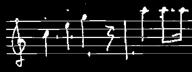
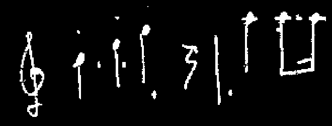
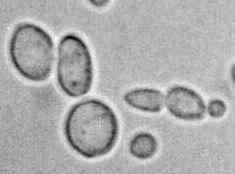
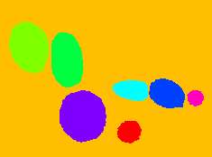
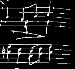
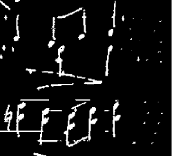
Image analysis and image understanding include basic image processing tasks such as segmentation and object detection. Many advances have been achieved recently in object detection with the use of supervised learning techniques, and particularly of convolutional neural networks [1, 2]. In object recognition, supervision is usually provided as labels attached to images or to regions in the images. In contrast, more lower level tasks such as segmentation require labels at pixel or superpixel levels [3]. For these type of tasks, the simplest way of providing supervision is by means of pairs of input-output images. For instance, Fig. 1 shows a sample of input and output images for the staff line removal problem and Fig. 2 shows an example for the cell segmentation problem. They illustrate respectively a binary segmentation and a multi-class segmentation problems. In both cases the pixel value in the output image can be taken as a pixel class label. There is a subtle difference in the nature of the transformation. In the first example, removal of staff lines can be seen as a component filtering transformation, resulting in binary output images (both input and output are images of the same nature). In the second case, although the output is still an image, its pixels values are labels and thus of a different nature of the input image. However, multiclass segmentation can be cast as a component detection plus component labeling problem, and its component detection part can be essentially represented by means of binary output images.

Figure 1: An example of input-output pair of images expressing the staff-line removal task.

Figure 2: An example of input-output pair of images expressing the cell segmentation task.

In this work we address problems where supervision is provided at the pixel level and the task is modeled as an image transformation. The approach proposed here is built on the image operator learning framework used along the years to address this type of problems [4, 5, 6]. This framework uses image operators that are translation-invariant and locally defined with respect to a finite non-empty window to model image transformations. Estimating these type of image operators from training data has been the subject of study since the 1990s [7, 5, 8], with some interesting results in binary image processing [6, 9]. Although here we restrict ourselves to binary image transformations (like the one in the first example above), modeling and concepts apply also to gray-scale image transformations. Application examples include documents [10, 4], comics [11], noise filtering [12, 8], retinal images [13, 14], diagrams [6], and others.

The problem of learning image operators is modeled as a problem of learning local transformations. While most earlier approaches valued morphological representation to favor interpretation [7, 5, 6], more recent approaches [13, 15, 14] drop the concern of explicitly keeping the morphological representation to favor efficiency provided by recent advances in machine learning techniques.

Still, a major limitation of most machine learning algorithms is input size, which in the context of image operator learning is determined by the window size. CNNs, on the other hand, can be trained with very large inputs. Therefore, in this work we propose the use of CNNs in the image operator learning framework. We are specially interested on how effective CNNs are when used in the context described above. As CNNs require adjustments of several parameters, another issue of interest is how much effort is required to tune the parameters. To address these issues, we consider the problem of removing staff-lines from music score images. This problem has been receiving attention recently [16, 17, 18] and there is a large public dataset with ground-truth information [16], making it interesting to our study. Moreover, there are performance reports of heuristic methods and also of learned image operators [9], which will allow us to make a direct comparison.

The rest of the paper is organized as follows. In Section II we describe the image operator learning framework [4], providing a brief but comprehensive overview. This overview will help to place the contributions of this work properly within the framework. In Section III we discuss how to couple CNNs to the above mentioned learning framework. In particular, we will define an experimental protocol to be followed to adjust the many parameters of a CNN model. Then, in Section IV we describe results on parameter determination and performance of the learned image operators. In Section V we present the conclusions of this work and comment on future works.

II Background

Although in practice images are defined on a finite support, to present some definitions and notations we consider they are defined on $\mathbb{E}=\mathbb{Z}^{2}$. A binary image defined on $\mathbb{E}$ is a function $f:\mathbb{E}\to\{0,1\}$, which can be represented equivalently by the set $S_{f}=\{\,p\in\mathbb{E}\,:\,f(p)=1\}$. To simplify notation, we will use the same symbol $S$ to denote a binary image both as a function and as a set. Thus, $S(p)=1$ and $p\in S$ has the same meaning. They both mean that the value of the image at point $p$ is 1. The collection of all binary images on $\mathbb{E}$ will be denoted $\mathcal{P}(\mathbb{E})$.

A binary image operator $\Psi:\mathcal{P}(\mathbb{E})\to\mathcal{P}(\mathbb{E})$ that satisfies translation-invariance and local definition w.r.t. a finite non-empty window $W$ (containing the origin of $\mathbb{E}$) can be expressed as

$$[\Psi(S)](p)=\psi(S_{-p}\cap W)$$ (1)

where $\psi$ is a function from $\mathcal{P}(W)$ to $\{0,1\}$ and $S_{-p}$ is the translation of image $S$ by $-p$.

This means that operators that satisfy both properties are fully defined by its characteristic function $\psi$. An interesting consequence of this property is that the problem of learning an image operator can be reduced to the problem of learning the characteristic function $\psi$ [4].

Given an input-output pair $(I,O)$ of training images, training data consists of image patches $I\cap W_{p}$, collected from $I$ by sliding window $W$ over every pixel $p$, together with its respective label $O(p)$. In practice, image patches are flattened and their vectorial form are used as inputs for training and classification [4].

Once a local function is learned, one can compute the output image by applying Eq. 1 on every point of an input test image. Given image pairs $(I_{i},O_{i})$, $i=1,\ldots,N$, the empirical mean absolute error (MAE) of $\psi$ is defined as

$$Err(\psi)=\frac{1}{T}\sum_{i=1}^{N}\sum_{p\in D(I_{i})}|\psi([I_{i}]_{-p}\cap W)-O_{i}(p)|$$ (2)

where $D(I)$ denotes the support of $I$ and $T$ the total of points considered in the summation. This error is equivalent to the pixel-wise accuracy.

Most previous works related to image operator learning use approaches that preserve the morphological representation of $\psi$. In the case of binary images, local functions are logical functions and they can be expressed as a sum of product terms [5, 6, 4]. Their corresponding morphological representation allows one to understand the learned operator in terms of basic morphological operators such as erosions, dilations and interval operators [19].

As window points can be regarded as variables (or features), there is a tradeoff between window size and generalization performance. Too small windows do not suffer from generalization error but their discriminatory power is limited. On the other hand, albeit having good discriminatory power, too large windows lead to poor generalization (small training error but large test error) [4].

One technique to overcome this limitation to learn operators defined w.r.t. larger windows is the two-level design approach [6]. This approach consists in designing multiple operators on moderate size windows and then taking the responses of each of them as second level features, which are then used to train a combiner. The combiner is, ultimately, an image operator that is locally defined w.r.t. a larger window (the union of all moderate size windows used in the first-level learning phase). Empirical analysis indicate that combinations consistently provide better results than single operators. A drawback of these approaches that are based on explicit morphological representation is the size complexity of such representations. The number of required elementary operators may be exponential to the window size [4].

More recent approaches take advantage of modeling and processing flexibility provided by modern machine learning algorithms [15, 14] and do not consider an explicit morphological representation. This represents a view shift in the modeling of image operator learning processes from approaches based on estimating local functions to approaches based on classifier learning. In classifier based approaches, image patches observed through $W$ take the place of input vectors $\mathbf{x}$, and the respective values in the output image take the place of class label $y$. Then, conventional classifier learning methods can be applied either directly on training samples $(\mathbf{x}_{i},y_{i})$ or on transformed ones $(\phi(\mathbf{x}_{i}),y_{i})$ (where $\phi$ is a feature transformation function).

III Proposed approach

We propose the use of CNNs as the classifier model to learn the local functions in the image operator learning framework described above. CNNs have some contrasting characteristics compared to previously used algorithms. First, CNNs are known by their ability to learn relevant features from data. Thus, they remove the need to handcraft and select suitable feature mappings $\phi$ for each application. In this sense, they form a generic method, but at the same time they possess the ability to encode problem specific knowledge. Second, CNNs can handle relatively large input images, managing generalization issues through supposedly powerful regularization techniques. Therefore, in our context they could be applied to learn local functions w.r.t. large windows (image patches) directly, rather than in multiple training phases as in the two-level approach proposed in [6]. Next we describe a method to obtain a CNN to be effectively used.

III-A Convolutional neural network architecture

A common issue when dealing with convolutional neural networks is the determination of an adequate architecture. A standard building block of CNNs is composed of convolution, ReLU and pooling layers, and a typical architecture of CNNs consists of multiple layers of these building blocks followed by fully connected layers. Some of the parameters that need to be defined before training are:

• input size: in our case, it is determined by the window size

• number of building blocks

• number of convolution masks in each block

• size of the convolution mask

• padding or no padding to compute the convolutions

• type of pooling

• number of fully connected layers

• cost function

• cost function optimization method, which may include dropout, and have varying learning rates and mini-batch sizes.

III-B Parameter evaluation

To avoid trying all possibilities for the parameters, which is clearly prohibitive, one can take the values used in similar works as reference. Since here we are dealing with binary images, at pixel classification level, there are only very few references. Thus, we opt to fix some of the parameters based on a preliminary evaluation and then evaluate the remaining parameters more carefully, as described below.

We have fixed a basic architecture consisting of two building blocks (i.e., convolution-ReLU-pooling layers) followed by two fully connected layers, and softmax output. The number of convolutions in each block is fixed to 32, and the mask size to $5\times 5$. We also adopt zero padding, stride 1 and max-pooling of $2\times 2$. For training, we use cross-entropy cost function along with the Adam algorithm [20], and stochastic gradient descend with mini-batch size of $50$ for optimization. We apply dropout regularization in the penultimate layer.

Given the fixed configuration above, we define an experimental protocol to evaluate the input window size, learning rate, and dropout rate. Note that the input window determines the image patches (raw input features) that will be used as input for training and classification of pixels. While most applications of CNN in the computer vision field consider a fixed input image size, window size is an important parameter in image operator learning [6].

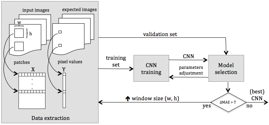
The strategy we follow to tune the CNN parameters is illustrated in Figure 3. For each window we evaluate multiple models, varying the value for the other parameters. This process is repeated for incremental window sizes. We start with a small window (in our case, $9\times 9$), as they are relatively faster to train and to provide feedback on the relevant ranges for the parameters. We then use the promising ranges to narrow the search range for larger windows. We use a validation set to evaluate the effects of distinct parameter values. Specifically, we have the following steps:

1. Grid search of parameters: We use the training set to train multiple instances of the basic CNN model above, varying the learning and dropout rates. For the smaller windows we first consider a coarse search on a wide range (for example, $[10,10^{-6}]$ for the learning rate); then we narrow the ranges according to the best parameters found, and do a finer search. For the larger windows, we start from the narrowed search ranges. For each training instance, we run 50 epochs, recording the CNN model after each epoch.

2. Model selection: The empirical mean absolute error (Eq. 2) of the $50$ CNN models of each training instance is computed on the validation set. Then, for each window size, the model with the lowest validation error is selected as the best model for that window.

We keep training CNNs over incremental window sizes until no considerable improvements are obtained. After the best CNN models per window are selected, we compare them and select the overall optimal one (the one with the lowest empirical MAE on the validation set).

Figure 3: CNN training and parameters evaluation. The input window size determines the patch size. We train and evaluate multiple CNN models over incremental window sizes. At each evaluated window size, we use the optimal parameters from smaller windows to narrow the parameters range.

A particular characteristic in image operator learning, and specially with respect to binary images, is the fact that many repeated patches may occur; indeed we can find cases where a same input patch has different expected labels (that is, cases where $\mathbf{x}_{i}=\mathbf{x}_{j}$ but $y_{i}\neq y_{j}$). Therefore, the total number of training patches may be much larger than the number of distinct patches, which can considerably reduce the training efficiency. Thus, for model selection we randomly selected subsets of the training samples. After the best model is selected, we train it again using the whole training set.

IV Experimentation

In this section we show the application of the proposed method (model selection and the performance of the selected model) on the problem of staff-line removal in music score images.

IV-A Experimental setup

We used the dataset of the ICDAR 2013 music scores competition: staff removal [16], as done in [9]. The dataset consists of handwritten music score images (with dimensions around $3400\times 2300$ pixels), modified in order to emulate degraded documents. The dataset is divided into training and test sets. Following [9], we selected 50 images for training and 20 for validation from the provided training set. From each image, we extracted patches centered at each white pixel of the image. The total number of patches extracted from the training and validation images was about $27$ and $10$ millions, respectively. To select the best model for each window, CNNs were trained using $5$ million patches randomly selected from the training set and evaluated also on $5$ million patches randomly selected from the validation set.

To evaluate the performance of the selected model, we measured accuracy, specificity, and recall on the test set, considering only the white pixels of the input images. In this setup, specificity measures the effectiveness of a method to preserve non-staff line pixels, and recall measures the effectiveness of the method to detect staff line pixels.

For implementing the CNNs, we used the TensorFlow library (http://tensorflow.org/) integrated with TRIOSlib, a library for image operator learning [4]. The implementations will be made available on the TRIOSlib project site (http://github.com/trioslib/trios).

IV-B Results on model selection

For all evaluated window sizes, best models were found using a learning rate in the $[10^{-5},10^{-6}]$ range, without significant variation when using larger or smaller windows. Also, the use of dropout did not considerably improved performance. This might be due to the fact that we did not use a very deep CNN.

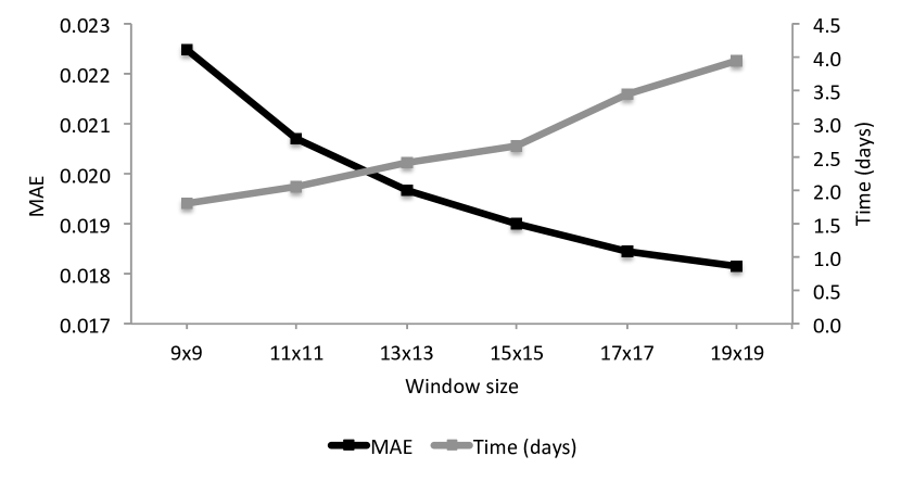
Figure 4 shows the MAE on validation set and the training time of the best CNN models per window size. We can see a small but consistent accuracy improvement, or MAE reduction, as the window size is incremented. However, such improvement also requires an increasing training time due to the larger input size. For instance, the training of all instances with the $9\times 9$ window took less than one day while with the $19\times 19$ window took about four days. All the experimentation was done on CPU only.

Figure 4: Mean absolute error (MAE, left hand axis) and training time (right hand axis) for the best CNN models per window size.

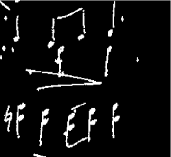
To understand the errors, we analyzed images with the largest errors. Figure 5 shows a region of one of such images, the same region in the expected output, and in the results obtained using the best CNN models with the $9\times 9$ and the $19\times 19$ windows. We have noticed that a common error is the misclassification of pixels of thick staff line segments as non-staff line pixels (the horizontal lines at the bottom-left part of the figures). Another type of error is on the extremities of the staff-lines. It can be seen that the errors are more evident in the output of the CNN with the smaller window.

(a)

(b)

(c)

(d)

Figure 5: Resulting image analysis: (a) region of an image for which CNNs obtained worst accuracy, (b) same region in the expected output image, and same region in the outputs produced by the best CNN models with (c) $9\times 9$ and (d) $19\times 19$ windows.

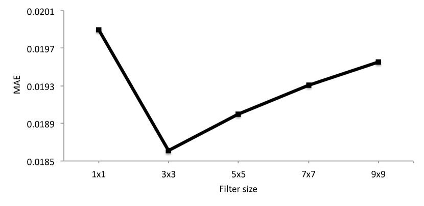
The convolution mask size was fixed to $5\times 5$ during model selection. As we intuitively reasoned that larger filters would allow CNNs to better capture staff line patterns, we did an experiment to evaluate this particular parameter for the case of $15\times 15$ window. We have found that higher accuracies are achieved with the $3\times 3$ mask, as shown in Figure 6. This indicates that additional study is necessary to undertand the effects of the convolution mask sizes on the results.

Figure 6: Mean absolute error (MAE) on validation set for different first layer filter sizes (window size fixed to $15\times 15$).

IV-C Performance of the selected model

According to the experiments in the model selection step, the best overall model was the best one in the group of those trained with $19\times 19$ window. The best model was retrained on the whole training set and evaluated on the test set. Table I shows the accuracy, specificity, and recall of the selected model as well as the ones provided in [9], which include results of four state-of-the-art methods. Three of the methods (LTC, Skeleton, LRDE) consist of heuristic techniques and the other (FS-MI) consists of a two-level operator learning approach with automatic window determination. Our method outperforms previous methods in terms of accuracy and recall, and also obtains the third best result in terms of specificity.

TABLE I: Performance comparison ($\%$) of our method with previous methods (performance of other methods extracted from [9]).

Method	Accuracy	Specificity	Recall
LTC	87.58	99.52	67.76
Skeleton	94.50	99.03	86.97
LRDE	97.03	98.84	94.02
FS-MI	96.96	98.46	94.48
Our method	97.96	98.98	95.72

IV-D Discussion

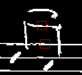
Although CNNs with larger windows have shown improved accuracy in comparison to CNNs with smaller windows, some pixels might not be correctly classified even using large windows. For instance, Figure 7 highlights two patches. The top one is on a beam note, capturing a horizontal line segment of the symbol. The second is centered on a staff line pixel. Visually they are very similar and the window required to distinguish them may be too large. A post processing of the output image might be an option to avoid using too large windows.

Figure 7: Some pixels might be difficult to classify by looking only at a local patch. The two highlighted patches are of size $19\times 19$ and are very similar each other, but they are in distinct classes.

Our best CNN model uses 361 features ($19\times 19$ windows), representing a large increment in the number of features compared to the classifiers used in [9] (40 features within a $13\times 17$ window domain). One advantage of the image learning framework is the fact that it is data-driven, adapting to the particularities of the considered family of images. This flexibility plus the ability of CNN on working with large inputs might be the explanation of superior results compared to previous methods.

V Conclusion

We introduced CNNs as local classifiers in the image operator learning framework. CNNs overcome limitations of previous methods with regard to practicable window sizes. In addition, CNNs remove the need of manually selecting features or combining simpler operators. This generality and flexibility comes accompanied with the challenge of finding an adequate set of CNN hyperparameters. We showed that by using standard architecture and parameter optimization methods, we obtain a CNN-based image operator that outperforms state-of-the-art staff line removal methods. Hence, we conclude that the use of CNNs as base classifiers in the image operator learning framework opens a promising path.

We note, however, that while the above statement fits well in scenarios where there is abundance of training data, there is still few knowledge regarding scenarios with few training data. Some of the issues to be further investigated include the application of the proposed method on images of different domains and also on gray-scale images. It would be interesting to test the limits of CNN (for instance, how far accuracy improvement can be pushed by augmenting the number of convolutional layers or window size?), adapt previously trained CNNs to other types of transformations, and understand which are the features extracted by CNNs.

References

- [1] A. Krizhevsky, I. Sutskever, and G. E. Hinton, “Imagenet classification with deep convolutional neural networks,” in Proceedings of the 25th International Conference on Neural Information Processing Systems (NIPS), USA, 2012, pp. 1097–1105.
- [2] R. Girshick, “Fast R-CNN,” in IEEE International Conference on Computer Vision (ICCV), 2015, pp. 1440–1448.
- [3] P. H. O. Pinheiro and R. Collobert, “From image-level to pixel-level labeling with Convolutional Networks,” in IEEE Conference on Computer Vision and Pattern Recognition (CVPR), 2015, pp. 1713–1721.
- [4] I. S. Montagner, N. S. T. Hirata, and R. Hirata Jr., “Image operator learning and applications,” in Conference on Graphics, Patterns and Images Tutorials (SIBGRAPI-T), 2016, pp. 38–50.
- [5] J. Barrera, E. R. Dougherty, and N. S. Tomita, “Automatic Programming of Binary Morphological Machines by Design of Statistically Optimal Operators in the Context of Computational Learning Theory,” Electronic Imaging, vol. 6, no. 1, pp. 54–67, 1997.
- [6] N. S. T. Hirata, “Multilevel training of binary morphological operators,” IEEE Transactions on Pattern Analysis and Machine Intelligence, vol. 31, no. 4, pp. 707–720, 2009.
- [7] E. R. Dougherty, “Optimal Mean-Square N-Observation Digital Morphological Filters I. Optimal Binary Filters,” CVGIP: Image Understanding, vol. 55, no. 1, pp. 36–54, 1992.
- [8] J. Yoo, K. L. Fong, J.-J. Huang, E. J. Coyle, and G. B. Adams III, “A Fast Algorithm for Designing Stack Filters,” IEEE Transactions on Image Processing, vol. 8, no. 8, pp. 1014–1028, August 1999.
- [9] I. S. Montagner, N. S. T. Hirata, and R. Hirata Jr., “Staff removal using image operator learning,” Pattern Recognition, vol. 63, pp. 310 – 320, 2017.
- [10] N. S. T. Hirata, J. Barrera, and R. Terada, “Text Segmentation by Automatically Designed Morphological Operators,” in Proc. of SIBGRAPI’2000, 2000, pp. 284–291.
- [11] N. S. T. Hirata, I. S. Montagner, and R. Hirata Jr., “Comics image processing: learning to segment text,” in Proc. of the 1st International Workshop on coMics ANalysis, Processing and Understanding. ACM, 2016, pp. 11:1–11:6.
- [12] E. J. Coyle and J.-H. Lin, “Stack Filters and the Mean Absolute Error Criterion,” IEEE Transactions on Acoustics, Speech and Signal Processing, vol. 36, no. 8, pp. 1244–1254, 1988.
- [13] M. E. Benalcázar, M. Brun, and V. L. Ballarin, “Artificial neural networks applied to statistical design of window operators,” Pattern Recognition Letters, vol. 34, no. 9, pp. 970 – 979, 2013.
- [14] I. S. Montagner, R. Hirata Jr, N. S. T. Hirata, and S. Canu, “Kernel approximations for W-operator learning,” in Conference on Graphics, Patterns and Images (SIBGRAPI), 2016, pp. 386–393.
- [15] I. S. Montagner, N. S. T. Hirata, R. Hirata Jr, and S. Canu, “NILC: a two level learning algorithm with operator selection,” in IEEE International Conference on Image Processing (ICIP), 2016, pp. 1873–1877.
- [16] M. Visaniy, V. Kieu, A. Fornes, and N. Journet, “ICDAR 2013 Music Scores Competition: Staff Removal,” in 12th International Conference on Document Analysis and Recognition (ICDAR), 2013, pp. 1407–1411.
- [17] C. Dalitz, M. Droettboom, B. Pranzas, and I. Fujinaga, “A comparative study of staff removal algorithms,” IEEE Trans. Pattern Anal. Mach. Intell., vol. 30, no. 5, pp. 753–766, 2008.
- [18] J. Calvo-Zaragoza, L. Micó, and J. Oncina, “Music staff removal with supervised pixel classification,” International Journal on Document Analysis and Recognition (IJDAR), vol. 19, no. 3, pp. 211–219, 2016.
- [19] H. J. A. M. Heijmans, Morphological Image Operators. Boston: Academic Press, 1994.
- [20] D. P. Kingma and J. Ba, “Adam: A method for stochastic optimization.” ICLR, 2014.