Nash equilibrium in a stochastic model of two competing athletes

Abstract

We propose a toy model for a stochastic description of the competition between two athletes of unequal strength, whose average strength difference is represented by a parameter $d$. The athletes interact through the choice of their strategies $x,y\in[0,1]$. These variables denote the amount of energy each invests in the competition, and determine the performance of each athlete. Each athlete picks his strategy based on his knowledge of his own and his competitor’s performance distribution, and on his evaluation of the danger of exhaustion, which increases with the amount of invested energy. We formulate this problem as a zero-sum game. Mathematically it is in the class of “discontinuous games” for which a Nash equilibrium is not guaranteed in advance. We demonstrate by explicit construction that the problem has a mixed strategy Nash equilibrium $\big{(}f(x),g(y)\big{)}$ for arbitrary $0<d<1$. The probability distributions $f$ and $g$ appear to both be the sum of a continuous component and a Dirac delta peak. It is remarkable that this problem is analytically tractable. The Nash equilibrium provides both the weaker and the stronger athlete with the best strategy to optimize their chances to win.

Keywords : Game theory; Stochastic processes; Exact results; Agent-based models

1 Introduction

The past decade has witnessed a growing use of the tools of statistical physics in order to understand human systems involving a form of competition [1], for example in a poker game [2], but also in sport (e.g. football [3], tennis [4, 5], baseball [6], or sport competitions in general [7]). A natural framework for describing a competition situation is provided by game theory. It has been applied, for example, to tournament competitions [8], or to pedestrians competing for going through a bottleneck [9, 10].

In this paper we focus on competition between two individual contestants that we will refer to as athletes. Our description is general and could apply to numerous different sports involving competition between individuals, such as swimming, cycling, rowing, skying, speed-skating. For definiteness we will place ourselves in the setting of running a race.

In the case of running, models at various levels of detail have been proposed to describe the supply of energy, both through anaerobic and aerobic metabolisms, that the athlete will be able to use during the race [11]. This energy supply, together with other parameters such as the propulsive force or possible friction forces, will determine a runner’s optimal velocity profile [12, 13, 14, 15] in the framework of optimal control theory, with good agreement with real world observations.

In a competition, interactions of several types may occur between the runners. For example, it seems that slipstreaming, well known for cycles, can also play a role in middle-distance running. An easy way to model this effect in the frame of optimal control is to assume that one of the athletes is running as if he were alone, and to optimize the trajectory of the other runner under the effect of slipstreaming [16]. However this approach treats the two athletes on a different footing. It is possible actually to propose models based on optimal control for which both trajectories are optimized simultaneously [17]. In any case, the solution (not necessarily unique) will be deterministic.

In reality the outcome of a race is uncertain due to the randomness of circumstances beyond the runners’ control. In the present paper we therefore introduce a stochastic model for a two-runner race, in which stochasticity can be seen as a modeling of the level of fatigue or motivation that can vary from one race to the next. We aim at presenting an exactly solvable model that illustrates principles, rather than retaining full realism. In our toy model, both runners are treated on equal footing. In particular, both are free to mutually adapt their strategies, and each of them does so with the purpose of winning as many races as possible. The stochasticity in the description opens in particular the possibility for the weaker athlete to win with a certain probability. The model will take the form of a game and we will therefore be able to apply the tools of game theory, whose essential points we will recall as we go along.

Assuming that the same two runners compete through a large number of races, we will find analytically a Nash equilibrium, that is a set of strategies such that none of the runners can increase his gain by changing unilaterally his strategy. We will show that in order to reach this Nash equilibrium, runners should not run all races the same way, but rather use mixed strategies so as to surprise their competitor.

In section 2 we define the model and express it in a form amenable to a game theoretic solution. In section 3 we show that if the model has a Nash equilibrium, this equilibrium consists necessarily of mixed strategies. In section 4 we briefly recall the symmetric case, well-known in the literature, in which the athletes are of equal strength. In section 5 we derive the main results of our work. We consider a weaker and a stronger athlete and show how this changes the nature of the symmetric solution. The full asymmetric solution is calculated analytically and commented upon. In section 6 we conclude and discuss some future perspectives.

2 A two-athlete model

2.1 Running times and energies

We consider two runners $R_{1}$ and $R_{2}$. For each race, we associate with $R_{i}$ a variable ${E}_{i}$  $(i=1,2)$, that we will refer to as his energy. When runner $R_{i}$ has an energy ${E}_{i}$, he will complete the race within his best final time $T({E}_{i})$, which we stipulate to be a decreasing function of its argument.

The introduction of this “energy”variable requires a short discussion. The runner’s best final time depends on several parameters, including various types of energy supplies (anaerobic, VO2) but also other physiological characteristics such as his maximal propulsive force or his friction coefficient. We refer to [14, 13, 15] for an analysis of how the final time depends on these parameters individually. The “energy” ${E}_{i}$  should be thought of as describing the integrated effect of all these parameters, in the spirit of the invested stamina introduced in [8]. Actually the variable ${E}_{i}$ could also simply be thought of as a way to parametrize the distribution of final times.

For each race, the energy ${E}_{i}$ available to runner $R_{i}$ is taken to be an independent stochastic variable drawn from a probability distribution $\rho_{i}({E}_{i})$. Each runner has a knowledge of the two energy distributions $\rho_{i}$ ($i=1,2)$ and thus knows in particular whether on average  he is stronger or weaker than his opponent. But on a given race, he can only make a guess about the actual  random values ${E}_{i}$ ($i=1,2)$ of the energies that are going to be available to himself and his opponent. Runner $R_{i}$ will therefore choose a value ${\epsilon_{i}}$ (his “strategy”) as a guess for the energy he expects to have available for this particular race.

Two scenarios are then possible. Either $R_{i}$ overestimated the energy available to himself (${\epsilon_{i}}>{E}_{i}$) and he will be exhausted before reaching the finish line; or he underestimated it (${\epsilon_{i}}\leq{E}_{i}$) and he will finish the race in a time $T({\epsilon_{i}})$. The probability of exhaustion associated with the choice of strategy ${\epsilon_{i}}$ is thus

$${P_{i}^{\rm exh}}=\int_{-\infty}^{\epsilon_{i}}\rho_{i}({E}_{i})\,\mbox{d}{E}_{i}\equiv\left\{\begin{array}[]{rr}x,&i=1,\\[5.69054pt] y,&i=2.\end{array}\right.$$ (1)

It is now clear how the interaction between runners comes into play. If a runner knows that he runs against a stronger competitor, he will tend to choose a higher ${\epsilon_{i}}$ in order to realize a shorter time $T({\epsilon_{i}})$, in spite of the increased risk of failing by exhaustion. If he knows he runs against a weaker opponent, he will choose a lower ${\epsilon_{i}}$ in order to reduce his risk of exhaustion.

Our term “exhaustion” should be understood in a broad sense. Indeed, in the same way as the variable ${E}_{i}$ represents the aggregation of several parameters, “exhaustion” also covers a variety of situations. For example, a lack of concentration can lead to a false start, athletes may suffer from various injuries, etc. Besides, exhaustion does not necessarily mean that the runner does not reach the finish line, but that he would do it (if at all) with a final time far less than the best time he could have expected (at least less than any best time $T({E}_{i})$ that the other runner can achieve). There are (rare) examples in the sport history where a weaker competitor indeed won a competition because other ones were eliminated for various reasons. For example, in the Olympic Games of Sydney in 2000, one Guinean swimmer won a race though it was the first time he was swimming in a 50 meter swimming pool, just because the other ones both made false starts [18].

We finally observe that this simplified model does not take into account any interactions between the two runners that might occur during  the race. Such more difficult questions are left for follow-up work.

2.2 Choice of the energy distributions $\rho_{i}({E}_{i})$

To simplify the calculations we will take for each $\rho_{i}({E}_{i})$ a uniform energy distribution on a unit interval. This interval will be $d\leq{E}_{1}\leq d+1$ for runner $R_{1}$ and $0\leq{E}_{2}\leq 1$ for runner $R_{2}$, as shown in Figure 1.

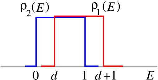
Figure 1: The energy distributions $\rho_{1}(E)$ and $\rho_{2}(E)$ of runners $R_{1}$ and $R_{2}$.

For $d=0$ there is symmetry between the two runners; for $d>0$ runner $R_{1}$ is the stronger one. Except when stated otherwise, we will consider only the case $0\leq d<1$, for which the weaker runner still has a nonvanishing probability to win. The case $d\geq 1$ is trivial in the sense that the stronger runner will always win.

For each race a stochastic variable ${E}_{i}$ (unknown to the runners) is chosen for each runner according to its distribution $\rho_{i}$. When we apply (1) for given guesses $\epsilon_{i}$ of the energies, we find that

$${P_{1}^{\rm exh}}=x=\epsilon_{1}-d,\qquad{P_{2}^{\rm exh}}=y=\epsilon_{2}\,.$$ (2)

Hence the choice of the strategy pair $(\epsilon_{1},\epsilon_{2})$ is equivalent to the choice of the pair $(x,y)$; since both $x$ and $y$ vary in the unit interval, these will be the most convenient variables for the calculations in later sections.

2.3 The resulting game

For a given strategy pair $(\epsilon_{1},\epsilon_{2})$ the possible outcomes of the race are listed in Table 1 together with their probabilities of occurrence. Four cases (first column of the table) must be distinguished, according to whether none, only $R_{1}$, only $R_{2}$, or both runners are exhausted before reaching the finish line. These cases occur with the probabilities listed in the second column of the table, and the winner is given by the third column. Indeed, when both runners reach the finish line without being exhausted, the winner is the one with the shorter time $T({\epsilon_{i}})$, hence the larger energy ${\epsilon_{i}}$; in case $\epsilon_{1}=\epsilon_{2}$, which is most of the time of measure zero as we shall see later, the winner is chosen randomly with probabilities $\frac{1}{2}(1\pm\gamma_{0})$ where, we introduced $\gamma_{0}\in[-1,1]$ as an additional parameter of the problem for reasons that will become clear later. When only one of the runners is exhausted, the other one wins. When both are exhausted, the winner is chosen uniformly randomly. There thus is always a winner and a loser.

Exhausted runners	Probability	Winner
none	(1-${P_{1}^{\rm exh}})(1-{P_{2}^{\rm exh}}$)	if $\epsilon_{1}>\epsilon_{2}$ : $R_{1}$
		if $\epsilon_{2}>\epsilon_{1}$ : $R_{2}$
		if $\epsilon_{1}=\epsilon_{2}$ : $R_{1}$ with probability $\frac{1}{2}(1+\gamma_{0})$
		if $\epsilon_{1}=\epsilon_{2}$ : $R_{2}$ with probability $\frac{1}{2}(1-\gamma_{0})$
$R_{2}$ only	$(1-{P_{1}^{\rm exh}}){P_{2}^{\rm exh}}$	$R_{1}$
$R_{1}$  only	${P_{1}^{\rm exh}}(1-{P_{2}^{\rm exh}})$	$R_{2}$
both	${P_{1}^{\rm exh}}{P_{2}^{\rm exh}}$	$R_{1}$ , $R_{2}$ with equal probability

Table 1: Race winner shown in four different cases of exhaustion and relative values of the $\epsilon_{i}$. The physical variables ${P_{1}^{\rm exh}},{P_{2}^{\rm exh}},\epsilon_{1}$, and $\epsilon_{2}$ may all be expressed in terms of $x$ and $y$ with the aid of Eq. (2).

We now model this race as a game by assigning a payoff $+1$ to the winner and $-1$ to the loser, which means that we have a zero-sum game. For a given strategy pair $(\epsilon_{1},\epsilon_{2})$ the expected  payoff for $R_{1}$, to be denoted as $G_{1}(\epsilon_{1}-d,\epsilon_{2})=G_{1}(x,y)$, is obtained as the sum on the probabilities for the four cases listed in Table 1, each weighted with $\pm 1$ according to whether runner $R_{1}$ is or is not the winner. Upon using Eq. (2) to express all quantities in terms of the variables $x$ and $y$ we find

Figure 2: The payoff function $G_{1}(x,y)$, defined on the unit square, is discontinuous along the dashed line separating regions I and II.

$$G_{1}(x,y)=\left\{\begin{array}[]{l l}-1+2y-xy,&x+d<y\quad\mbox{ (region II),}\\[5.69054pt] \phantom{-}1-2x+xy,&x+d>y\quad\mbox{ (region I),}\\[5.69054pt] \phantom{-}d+\gamma(x),&x+d=y,\end{array}\right.$$ (3)

with $(x,y)\in[0,1]^{2}$ and in which

$$\gamma(x)=\gamma_{0}\,(1-x)(1-x-d)$$ (4)

defines the payoff on the line of discontinuity. For $\gamma_{0}=0$ this payoff takes the value $d$, halfway between the neighboring values in the regions I and II (see Figure 2). For $\gamma_{0}=1$ [for $\gamma_{0}=-1$] the value $d+\gamma(x)$ is equal to the limit of $G_{1}(x,y)$ as the discontinuity is approached in region I [in region II], so that $G_{1}$ is upper (lower) semi-continuous.

Since the race is a zero-sum game, the expected gain $G_{2}(y,x)$ of runner $R_{2}$ is

$$G_{2}(y,x)=-G_{1}(x,y).$$ (5)

Eq. (3) together with (5) defines the “game.”

We will now address the question of determining the best strategies for $R_{1}$ and $R_{2}$ if each wants to maximize his payoff. This is the subject of the next sections.

3 Nonexistence of a Nash equilibrium of pure strategies

Having defined the game (3), we now ask what the best strategy is for each runner and will appeal to game theory to find the answer.

In general, a strategy will be mixed, that is, each time the race is repeated, runner $R_{1}$ chooses an $x$ from a distribution $f(x)$ and runner $R_{2}$ a $y$ from a distribution $g(y)$. A pure  strategy is the special case in which a runner always chooses the same $x=x_{0}$ or $y=y_{0}$ (hence $f$ or $g$ is a Dirac delta function). A Nash equilibrium is a pair of strategies $(f(x),g(y))$ such that neither runner can improve his payoff by a unilateral change of strategy. A general game may have no such equilibrium, or a unique one, or several.

We will now show that (3) does not have a Nash equilibrium of pure strategies. For a zero-sum game, game theory tells us that a Nash equilibrium coincides with a minimax solution. The idea of a minimax solution is that each player will try to minimize his worst-case loss, or equivalently that he will try to maximize his worst-case gain. When we restrict ourselves to pure strategies, this means that runner $R_{1}$ will play the strategy $x^{*}$ that ensures he will win at least $G^{*}_{1}=\max_{x}\left[\min_{y}G_{1}(x,y)\right]$ and runner $R_{2}$ will play the strategy $y^{*}$ that ensures he will lose at most $-G^{*}_{2}=\min_{y}\left[\max_{x}G_{1}(x,y)\right]$. If $G_{1}^{*}$ and $G_{2}^{*}$ exist, then necessarily

$$G^{*}_{1}=\max_{x}\min_{y}G_{1}(x,y)\leq\min_{y}\max_{x}G_{1}(x,y)=-G^{*}_{2}$$ (6)

If, moreover, for a pair $(x^{*},y^{*})$ of strategies Eq. (6) holds as an equality, then this pair is a minimax solution and is also a Nash equilibrium. Inversely, if there exists a pure strategy Nash equilibrium, then $G_{1}^{*}$ and $G_{2}^{*}$ should both exist and be equal.

For our present problem, and for $0\leq d<1$, one shows with the aid of a short calculation that

$$\sup_{x}\inf_{\rule{0.0pt}{7.25545pt}y}G_{1}(x,y) = d-\Delta,\noindent$$ (7)

$$\inf_{\rule{0.0pt}{7.25545pt}y}\sup_{x}G_{1}(x,y) = d+\Delta,\qquad\Delta\equiv 3-\sqrt{8+d^{2}},$$ (8)

which excludes the possibility for Eq. (6) to be satisfied with the equality sign. Hence we see that there cannot be a Nash equilibrium of pure strategies. We have relegated the proof of (8) to A, where we show that the extrema are reached at the point $(x^{*},x^{*}+d)$ with $x^{*}=(4-d-\sqrt{8+d^{2}})/2$, located on the line of discontinuity, and that the difference $2\Delta$ between the two expressions in (8) is equal to the jump of $G_{1}$ across the discontinuity in that point.

In the absence of a pure strategy Nash equilibrium, the next step is to look for one with mixed strategies. The fact that in our game there is a discontinuity will turn out to be mathematically essential and we will therefore treat the line $x+d=y$ discontinuity with the care required. Glicksberg’s theorem (as cited by [19]) guarantees the existence of a Nash equilibrium for a discontinuous game only if $G_{1}(x,y)$ is upper or lower semicontinuous. The game (3) lacks this property for all $\gamma_{0}\in(-1,1)$, but we will show by explicit construction that it nevertheless does have a Nash equilibrium.

4 Symmetric problem

We take in this section $d=0$, so that we have two runners of equal strength, $R_{1}$ and $R_{2}$, with respective strategies $x,y\in[0,1]$. The (positive or negative) gain of $R_{1}$ is given by the payoff function

$$G_{1}(x,y)=\left\{\begin{array}[]{ll}-1+2y-xy,&x<y,\\[5.69054pt] \phantom{-}1-2x+xy,&x>y,\\[5.69054pt] \phantom{-}\gamma_{0}(1-x)^{2},&x=y,\end{array}\right.$$ (9)

and the gain of $R_{2}$ is the opposite, $G_{2}(y,x)=-G_{1}(x,y)$. This game (with $\gamma_{0}=0$) is a classical textbook example [20]. We briefly recall how its Nash equilibrium is obtained. Since we found in section 3 that this problem has no Nash equilibrium of pure strategies, we will now look for one in which $R_{1}$ and $R_{2}$ have mixed strategies with identical distributions $f(x)$ and $f(y)$, respectively, that satisfy

$$f(z)\geq 0,\qquad\int_{0}^{1}{\rm d}z\,f(z)=1.$$ (10)

The support of $f(z)$ may be smaller than the full interval $[0,1]$. One may try to solve the problem by supposing that the support is an interval $[0,a]$ with an as yet unknown $a\in(0,1)$.

If runner $R_{1}$ chooses a strategy $x$ in the support of $f(x)$, then his expected payoff averaged over $R_{2}$’s mixed strategy $f(y)$ will be

$$\overline{G}_{1}[x;f(y)]=\int_{0}^{a}{\rm d}y\,G_{1}(x,y)f(y).$$ (11)

As a consequence of the definition of a Nash equilibrium, the mixed strategy $f(y)$ that we are looking for should be such that

$$\overline{G}_{1}[x;f(y)]=K,\qquad 0\leq x\leq a,$$ (12)

where $K$ is some constant. Indeed, if a specific strategy $x=x_{0}$ would yield a payoff less than $K$ to runner $R_{1}$, then $R_{1}$ would remove that $x_{0}$ from the support of $f(x)$; and if a specific strategy $x=x_{0}$ would yield a payoff larger than $K$ to runner $R_{1}$, then $R_{1}$ could improve his expected payoff by putting a larger weight on that $x_{0}$ – both in contradiction with the definition of a Nash equilibrium. By symmetry we must of course in the end find $K=0$, but we have not needed that here.

It is not a priori  clear how many solutions there are to (12), if any at all. We will look for an $f$ that is differentiable. When we substitute (11) in (12), use the explicit expression (9) for the payoff function, and differentiate twice with respect to $x$, there arises a first order ODE for $f(y)$ whose solution is

$$f(y)=\frac{D(a)}{(1-y)^{3}}\,,\qquad 0\leq y\leq a.$$ (13)

Normalization yields $D$ as a function of the hypothesized interval parameter $a$,

$$D(a)=\frac{2(1-a)^{2}}{a(2-a)}\,.$$ (14)

In order to determine $a$ we substitute (13) in the original expression (12), which leads to

$$K=\frac{(3a-2)D}{2(1-a)^{2}}\left[a-(2-a)x\right],\qquad 0\leq x\leq a.$$ (15)

We should now render the RHS of (15) independent of $x$. As $a$ cannot be equal to $2$ (we have $a<1$), the only way this condition can be met is when the prefactor $3a-2$ vanishes. Then $K=0$ as expected and $a=\frac{2}{3}$, which combined with (14) yields $D=\frac{1}{4}$. The resulting function $f(x)=1/[4(1-x)^{3}]$ is shown in Figure 3. To make sure that it actually represents a Nash equilibrium, one also has to show that neither runner can improve his result by choosing a strategy outside of the support $[0,a]$. This is easily done [20]. Finally we observe that the value of $G_{1}(x,y)$ on the discontinuity line has played no role here: the equilibrium is independent of $\gamma_{0}$.

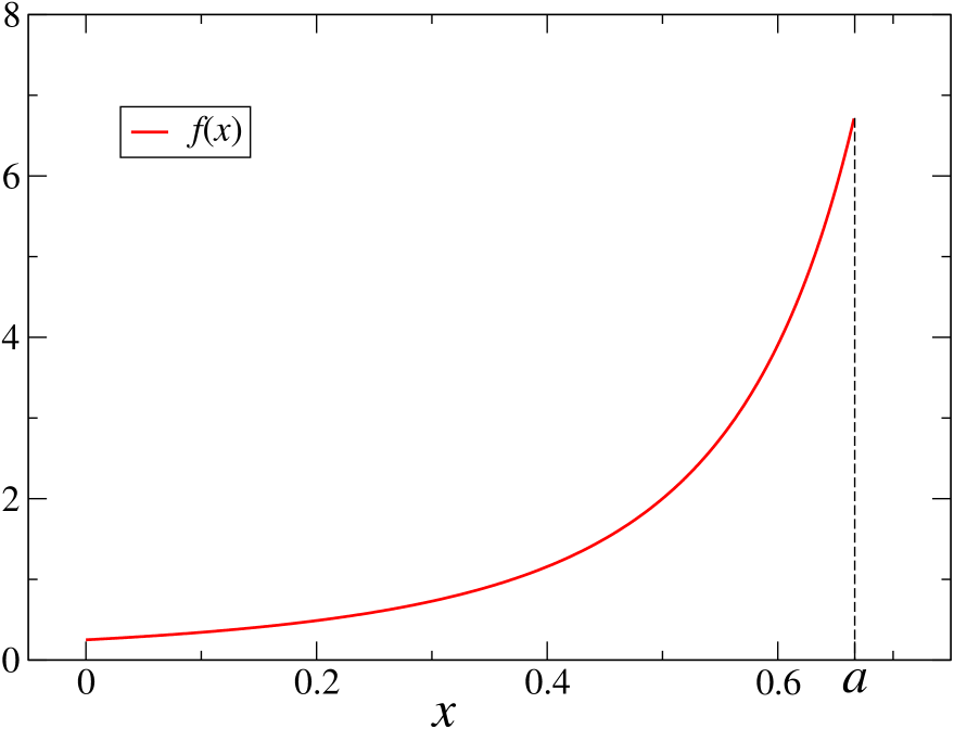
Figure 3: The function $f(x)$ representing the Nash equilibrium for the symmetric problem, $d=0$. Here $a=\frac{2}{3}$.

5 Asymmetric problem

The case of asymmetric runners has not so far been studied, and doing so is the purpose of this work. The question of whether a discontinuous game has or does not have a Nash equilibrium is the subject of several mathematical theorems, but has not received an exhaustive answer. Glicksberg’s theorem applies here only for $\gamma_{0}=\pm 1$. We don’t know either whether the solution is unique. We will show below that for the problem at hand such a solution does exist by calculating it explicitly. It is remarkable that this problem may be solved analytically exactly, as there is no general method allowing to systematically find Nash equilibria.

5.1 The asymmetric problem and the ansatz  for its solution

For an asymmetry parameter $d>0$ defined in section 2.3 the payoff function $G_{1}(x,y)$ that gives runner $R_{1}$’s gain is given by the general expression Eq. (3), which we repeat here for easy reference,

$$G_{1}(x,y)=\left\{\begin{array}[]{ll}-1+2y-xy,&x+d<y,\\[5.69054pt] \phantom{-}1-2x+xy,&x+d>y,\\[5.69054pt] \phantom{-}d+\gamma(x),&x+d=y.\end{array}\right.$$ (16)

The gain of runner $R_{2}$ is again equal to $R_{1}$’s loss, that is, $G_{2}(y,x)=-G_{1}(x,y)$. We note that the payoff function (16) differs from the one of the symmetric case, Eq. (9), only by a parallel shift of the line of discontinuity. In this case we have to solve the full asymmetric game, that is, assume that runners $R_{1}$ and $R_{2}$ have distinct strategies $f(x)$ and $g(y)$, respectively. Their expected gains $\overline{G}_{1}[x;g(y)]$ and $\overline{G}_{2}[y;f(x)]$ have the expressions

$$\overline{G}_{1}[x;g(y)] = \int_{{\rm supp}\,g}{\rm d}y\,G_{1}(x,y)g(y),$$ (17)

$$\overline{G}_{2}[y;f(x)] = \int_{{\rm supp}\,f}{\rm d}x\,G_{2}(x,y)f(x).$$ (18)

and we must consider the pair of equations

$$\overline{G}_{1}[x;g(y)]=\ \ K,\qquad x\in\mbox{supp }f,$$ (19)

$$\overline{G}_{2}[y;f(x)]=-K,\qquad y\in\mbox{supp }g.$$ (20)

As $R_{1}$ is now stronger than $R_{2}$, we anticipate that $K>0$.

There is no general method to determine $f$ and $g$. In the preceding section we assumed that the solution $f=g$ was differentiable, and it appeared that indeed such a solution existed; but this need not always be the case. In the asymmetric case two arguments can help us to guess the forms of $f$ and $g$. First, the solution to the symmetric problem given above suggests that $f$ and $g$ will at least each have a differentiable component, in addition to anything else. Secondly, we have used the online solver of Avis et al. [21] to obtain the exact Nash equilibrium for a version of the system in which each strategy was confined to a set of fifteen discrete points, with the points of the two sets alternating along the axis.

Inspired by these considerations we decided to look for strategies $f(x)$ and $g(y)$ that both have a differentiable component and, at the lower end of the allowed strategy interval, a Dirac delta peak. That is, we make the ansatz

$$f(x) = q_{1}\delta(x)+(1-q_{1})f_{\rm c}(x),\qquad 0\leq x\leq 1,$$ (21)

$$g(y) = q_{2}\delta(y)+(1-q_{2})g_{\rm c}(y),\qquad 0\leq y\leq 1,$$ (22)

where $f_{\rm c}$ and $g_{\rm c}$ are differentiable and have their support on an interval $\epsilon_{1},\epsilon_{2}\in(d,d+a]$, that is common to both runners on the original energy axis. Here again, the interval length $a$ is as yet unknown but should be such that $0<a\leq 1-d$. In terms of the variables $x$ and $y$ this “common” interval is given by

$$0<x\leq a,\qquad d<y\leq d+a.$$ (23)

Hence

$$f_{\rm c}(x),\ g_{\rm c}(y)>0,\qquad\int_{0}^{a}\mbox{d}x\,f_{\rm c}(x)=\int_{d}^{d+a}\mbox{d}y\,g_{\rm c}(y)=1.$$ (24)

A schematic representation of the space of possible strategies is given in Figure 4.

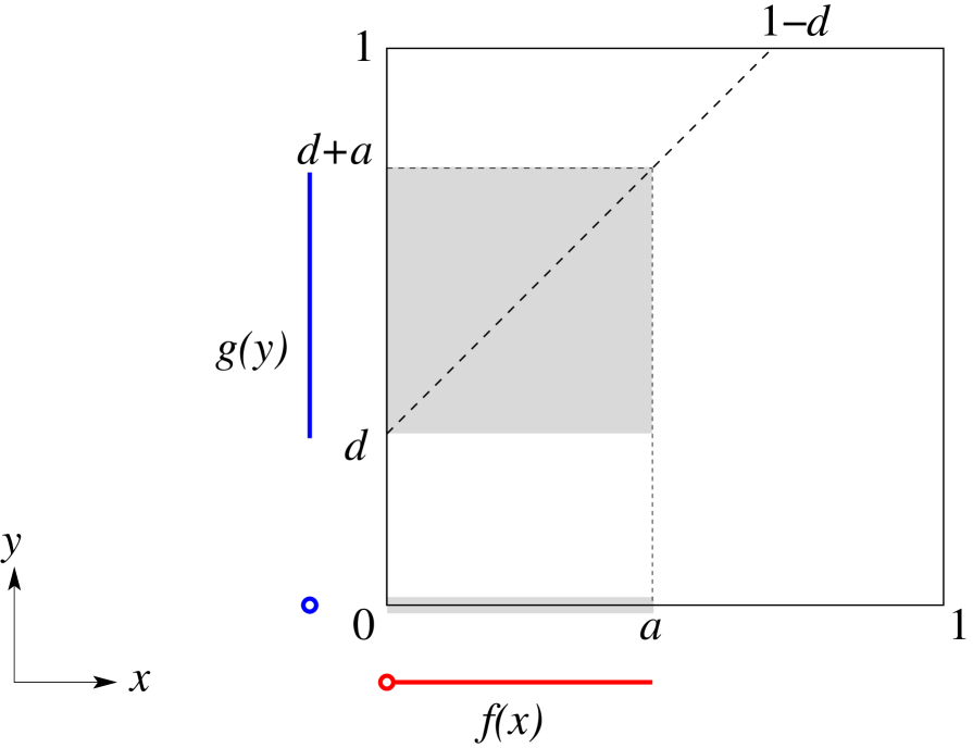
Figure 4: The space of possible strategies is the unit square. The payoff function $G_{1}(x,y)$ is discontinuous along the dashed line parallel to the diagonal. The Nash equilibrium is a pair $\big{(}f(x),g(x)\big{)}$. The heavy red line, when projected vertically onto the $x$ axis, gives the support of $f(x)$; similarly, the heavy blue one, when projected horizontally onto the $y$ axis, gives the support of $g(y)$. The red and blue circles denote the location of Dirac delta function components. The one of $g(y)$ is isolated from the rest of its support. The effectively used strategy pairs $(x,y)$ in the Nash equilibrium are limited, therefore, to the subspace $[0,a]\times\Big{(}\{0\}\cup(d,d+a]\Big{)}$ that has been shaded and consists of a square and a line interval.

5.2 Determining $f_{\rm c}(x)$, $g_{\rm c}(y)$, $q_{1}$, $q_{2}$, and the interval length $a$

We proceed to find a pair of strategies $f(x)$ and $g(y)$ having the hypothesized form (21)-(22).

Upon substituting Eqs. (21) and (22) in Eqs. (18) and (17), respectively, we obtain

$$\overline{G}_{1}[x;g(y)] = q_{2}G_{1}(x,0)+(1-q_{2})\int_{d}^{d+a}\mbox{d}y\,G_{1}(x,y)g_{\rm c}(y),$$ (25)

$$0\leq x\leq a$$

and, using the zero-sum property (5) to eliminate $G_{2}$ in favor of $G_{1}$ ,

$$\overline{G}_{2}[y;f(x)] = -q_{1}G_{1}(0,y)-(1-q_{1})\int_{0}^{a}\mbox{d}x\,G_{1}(x,y)f_{\rm c}(x),$$ (26)

$$y=0\ \ \mbox{ or }\ \ d<y\leq d+a.$$

On the RHS of these equations the contribution of the Dirac deltas are respectively $G_{1}(x,0)=1$ and $G_{1}(0,y)=-1+2y$. In the integrals appearing in Eqs. (25)-(26), we now use the explicit expression (16) for $G_{1}(x,y)$. This leads to splitting both intervals of integration into two subintervals separated by a point of discontinuity at $x+d=y$. The value $G_{1}(x,x+d)=d+\gamma(x)$ of the payoff at  the discontinuity has zero weight under the integrals and does not affect the outcome. Note that in Eq. (26) the particular value $y=d$, which is outside the support of $g(y)$, is excluded. As a consequence the value of the payoff on the line of discontinuity has not so far appeared in any of our considerations.

When differentiating (25) twice with respect to $x$ and (26) twice with respect to $y$, we find for $f_{\rm c}(x)$ and $g_{\rm c}(y)$ the linear first order ODEs

$$f^{\prime}_{\rm c}(x)=\frac{3-d-3x}{(1-x)(1-d-x)}f_{\rm c}(x),\quad g^{\prime}_{\rm c}(y)=\frac{3+d-3y}{(1-y)(1+d-y)}g_{\rm c}(y),$$ (27)

in which the parameters $q_{1}$, $q_{2}$, and $K$ no longer appear. The solutions are

$$f_{\rm c}(x) = \frac{B(a)}{(1-d-x)^{2}(1-x)}\,,\qquad 0<x\leq a,$$ (28)

$$g_{\rm c}(y) = \frac{D(a)}{(1+d-y)^{2}(1-y)}\,,\qquad d<y\leq d+a,$$ (29)

and vanish outside the intervals indicated. Normalization yields $D$ and $B$ in terms of the interval length $a$,

$$D^{-1}(a) = \phantom{-}{\cal L}(a)-\frac{a}{d(1-a)}\,,$$ (30)

$$B^{-1}(a) = -{\cal L}(a)+\frac{a}{d(1-d)(1-d-a)}\,,$$ (31)

with the abbreviation

$${\cal L}(a)=\frac{1}{d^{2}}\log\frac{(1-d)(1-a)}{1-d-a}\,.$$ (32)

Figure 5 shows the functions $f(x)$ and $g(y)$ of Eqs. (21)-(22) with $f_{\rm c}(x)$ and $g_{\rm c}(y)$ given by (28)-(29) for the special case of asymmetry parameter $d=\frac{1}{3}$ and with $a$, $q_{1}$, and $q_{2}$ having the values that will be determined below.

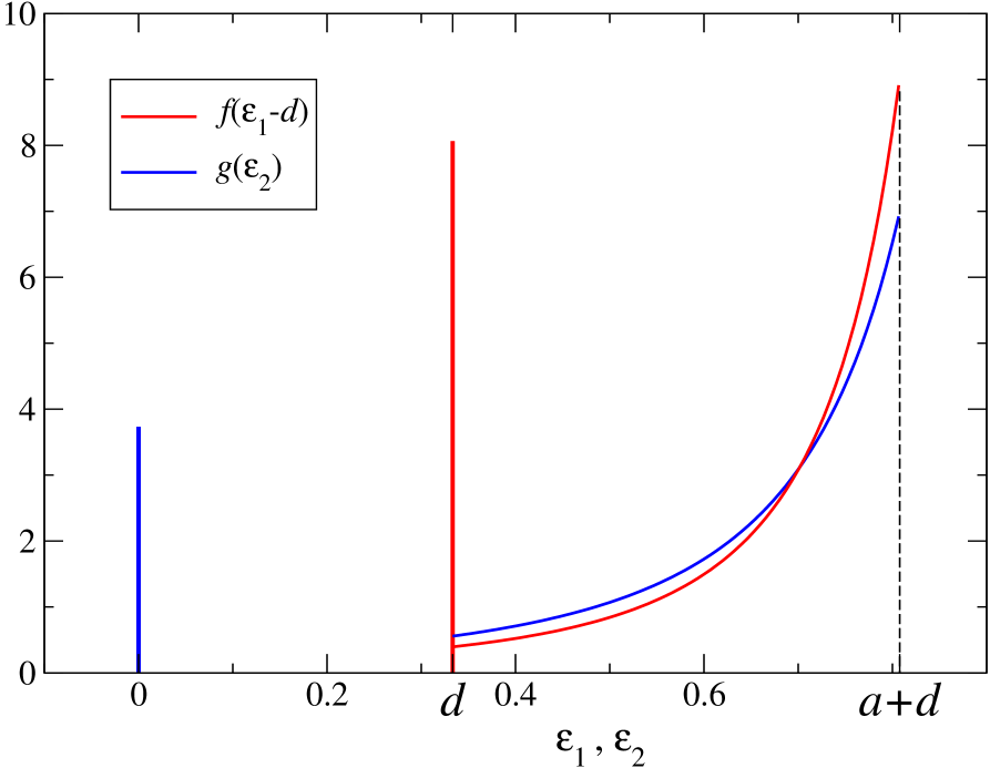
Figure 5: The two strategies for asymmetry parameter $d=\frac{1}{3}$ as functions of the energies $\epsilon_{1}=x+d$ and $\epsilon_{2}=y$. Each vertical bars represents the value of the integrated delta function at that point, multiplied by 100. The continuous components of the strategies are $f_{\rm c}(x)$ (red curve) and $g_{\rm c}(y)$ (blue curve). The right hand limit point of the support is at $a+d=0.4743799+\frac{1}{3}=0.8077132$.

At this stage the unknown parameters are $a,q_{1},q_{2},$ and $K$, the last three of which have been eliminated by the differentiations carried out above. To determine these we have to substitute the solutions (28) and (29) in the original equations (26) and (25) and then impose (19) and (20).

5.2.1 Substitution in (26).

Once (28) has been substituted in (26) and the integrals have been carried out explicitly, we find that $\overline{G}_{1}[x;g(y)]$ becomes a linear expression in $x$. The equality $\overline{G}_{1}[x;g(y)]=K$ then leads to two conditions from which $q_{2}$ and $K$ may be solved in terms of $a$. The result is

$$q_{2}=\frac{A_{D}}{A_{D}-1}$$ (33)

with

$$A_{D}=\frac{1}{2}-\frac{(2-a)D}{2(1-a)}\,,$$ (34)

and

$$K=1-(1-q_{2})\frac{2aD}{1-a}\,.$$ (35)

When (33) together with (34) is substituted in (35), this yields an expression for $K$ solely in terms of $a$, the normalization constant $D$ whose $a$ dependence is given by (30), and the asymmetry parameter $d$.

5.2.2 Substitution in (25).

Once (29) has been substituted in (25) and the integrals have been carried out explicitly, we similarly find that $\overline{G}_{2}[y;f(x)]$ becomes a linear expression in $y$. The equality $\overline{G}_{2}[y;f(x)]=-K$ then leads to two conditions from which $q_{1}$ and $K$ may be solved in terms of $a$. A third condition arises from the requirement that also for $y=0$ we must have $\overline{G}_{2}[0;f(x)]=-K$. It turns out, however, that this third condition is satisfied when the former two are. The result is

$$q_{1}=\frac{A_{B}}{A_{B}+1}$$ (36)

with

$$A_{B}=-\frac{1}{2}+\frac{B(2-2d-a)}{2(1-d)(1-d-a)}\,,$$ (37)

and

$$K=2d-1-(1-q_{1})\Big{[}d-\frac{(2-d)aB}{(1-d)(1-d-a)}\Big{]}.$$ (38)

When (36) together with (37) is substituted in (38), this yields again an expression for $K$ solely in terms of $a$, the normalization constant $B$ whose $a$ dependence is given by (31), and the asymmetry parameter $d$.

5.2.3 Combining the two substitutions.

The interval length $a$ is fixed by the condition that the two expressions for $K$, (35) and (38), be equal. After division by $BD$ this condition takes the form

$$\frac{2a(2-d-a)}{(1-d)(1-a)(1-d-a)}+\frac{a}{(1-d)(1-d-a)}\,\frac{1}{D}-\frac{2}{B}-\frac{1}{BD}=0.$$ (39)

Upon substituting in (39) the explicit results (30)-(31) for $D^{-1}$ and $B^{-1}$ we obtain a quadratic expression in the logarithm ${\cal L}(a)$ of Eq. (32) with coefficients that are ratios of low-degree polynomials in $a$ and $d$. One may show by tedious work that this expression can be factorized and that (39) reduces to

$$\Big{[}(1-a)d\,{\cal L}(a)-a\Big{]}\Big{[}(1-d-a)d\,{\cal L}(a)-(2d+1)a-2d(d-1)\Big{]}=0.$$ (40)

The first factor in (40) does not have a zero in the interval $0<a<1-d$. It thus appears that the “physical” solution is obtained by setting the second factor equal to zero. The resulting equation, slightly rewritten and exponentiated, becomes

$$-{\rm e}^{-(2d^{2}+1)}\,=\,-\frac{(1-d)(1-a)}{1-d-a}\,{\rm e}^{-\frac{(1-d)(1-a)}{1-d-a}},$$ (41)

which is of the form $Y=X{\rm e}^{X}$ with $Y=-\exp\big{(}-(2d^{2}+1)\big{)}$ and $X=-(1-d)(1-a)/(1-d-a)$. The solution is $X={\cal W}(Y)$ where ${\cal W}$ is the Lambert function. For negative $X$, as is our case, it has two branches, ${\cal W}_{0}$ and ${\cal W}_{-1}$; requiring that $0<a<1-d$ leads us to identify the “$-1$” branch as the “physical” one. Hence we have

$$-\frac{(1-d)(1-a)}{1-d-a} = {\cal W}_{-1}\big{(}-{\rm e}^{-(2d^{2}+1)}\big{)}$$ (42)

$$\equiv -w\,,$$

where the second line defines $w$. The number $w$ is positive and as $d$ varies it is in the interval $w\in[-{\cal W}_{-1}(-{\rm e}^{-1}),-{\cal W}_{-1}(-{\rm e}^{-3})]=[1,4.505241]$, the lower and upper limits occurring for $d=0$ and $d=1$, respectively. Eq. (42) now shows that the hitherto unknown interval length $a$ is given by the elegant expression

$$a=\,\frac{(1-d)(1-w)}{1-d-w}\,.$$ (43)

Figure 6 shows the behavior of $a$ as a function of $d$. It appears that for $d\to 0$ the solution of the symmetric problem with $a=2/3$ is recovered.

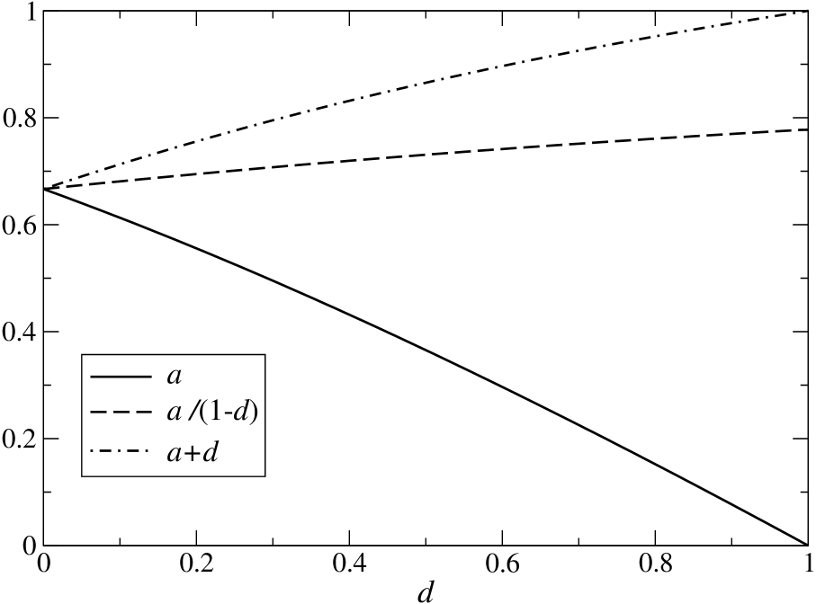
Figure 6: Interval length $a$, scaled interval length $a/(1-d)$, and the sum $a+d$ as a function of the asymmetry parameter $d$.

Figure 7 shows the expected gain $K$ of runner $R_{1}$ as a function of $d$. The values $K=0$ and $K=1$ correspond to runner $R_{1}$ winning with probability $\frac{1}{2}$ and $1$, respectively. The increase with $d$ appears to be almost, but not completely, linear.

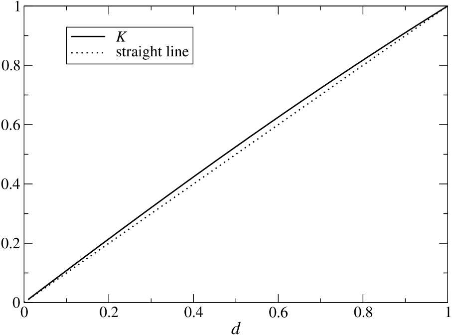
Figure 7: Expected gain $K$ of runner $R_{1}$ (the stronger one) as a function of the asymmetry parameter $d$. The dotted straight line is shown for comparison.

Figure 8 shows the coefficients (integrated values) $q_{1}$ and $q_{2}$ of the delta peaks in the strategies, as a function of the asymmetry parameter $d$. For $d\to 0$ the amplitudes of the delta functions vanish and the solution of the symmetric problem is recovered.

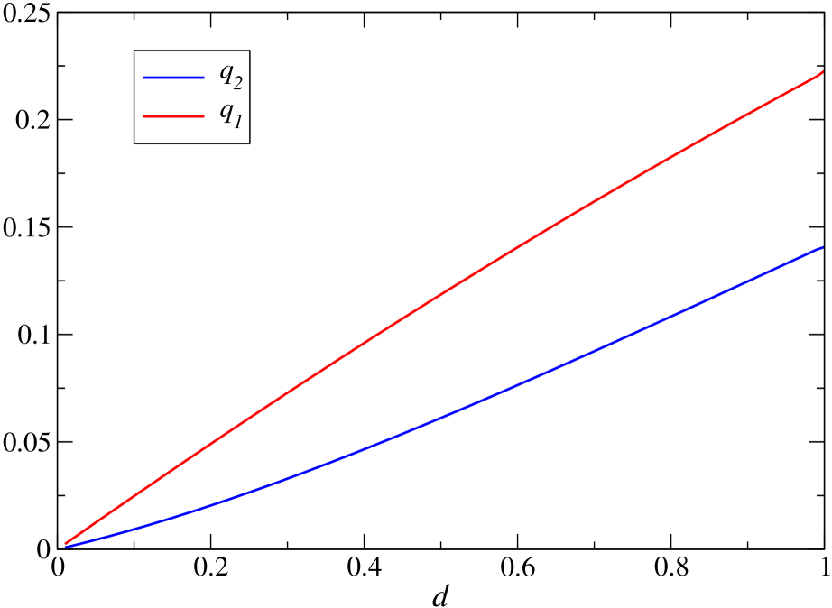
Figure 8: Coefficients $q_{1}$ and $q_{2}$ of the Dirac deltas in Eqs. (21) and (22) as functions of the asymmetry parameter $d$.

Figure 5 shows, for the special value $d=\frac{1}{3}$, the strategies $f(x)$ and $g(y)$ that are the main result of this report. We have plotted them as functions of the energies $\epsilon_{1}=x+d$ and $\epsilon_{2}=y$. Each strategy consists of a continuous part and a Dirac delta. The delta functions have been presented as vertical bars of height equal to 100 times their integrated value in the corresponding point, viz. $x=0$ for $f(x)$ and $y=-\frac{1}{3}$ for $g(y)$.

In summary, we found a pair of functions $f(x)$ and $g(y)$ given by Eqs. (21) and (22), (28)-(32) for $f_{\rm c}(x)$ and $g_{\rm c}(y)$, Eqs. (33)-(34) and (36)-(37) for the parameters $q_{2}$ and $q_{1}$, respectively, in which finally the interval length $a$ is fixed by Eqs. (42)-(43).

5.3 Completing the proof

In order to complete the proof that this pair is a Nash equilibrium, we have to show that neither player can improve his gain by choosing a strategy outside of the support of the functions ($f(x)$ for $R_{1}$ and $g(y)$ for $R_{2}$) obtained above. That is, we must show that

$$\overline{G}_{1}[x;g(y)]\leq\ \ K,\qquad x\notin\mbox{supp }f,$$ (44)

$$\overline{G}_{2}[y;f(x)]\leq-K,\qquad y\notin\mbox{supp }g,$$ (45)

which complement Eqs. (19)-(20). We will prove Eqs. (44)-(45) below.

Let us first consider runner $R_{1}$ and suppose that he chooses a strategy $x\in(a,1]$. Then his expected gain is

$$\overline{G}_{1}[x;g(y)] = q_{2}G_{1}(x,0)+(1-q_{2})\int_{d}^{a+d}\mbox{d}y\,G_{1}(x,y)g_{\rm c}(y)$$ (46)

$$= q_{2}(1-2x)+(1-q_{2})\int_{d}^{a+d}\mbox{d}y\,(1-2x+xy)g_{\rm c}(y),$$

where the expression for $G_{1}(x,y)$ is a consequence of the fact that here $x>a$ and $y\leq a+d$, whence $x+d>y$. Figure 4 is helpful to visualize these various inequalities. Expression (46) is clearly strictly decreasing with $x$ and therefore

$$\overline{G}_{1}[x;g(y)]<\overline{G}_{1}[a;g(y)]=K\qquad\mbox{ for }x\in(a,1],$$ (47)

which means that (44) is satisfied.

Let us next consider runner $R_{2}$. Three cases may occur.

Case 1. If $R_{2}$ chooses a strategy $y\in(a+d,1]$, his expected gain is

$$\overline{G}_{2}[y;f(x)] = -q_{1}G_{1}(0,y)-(1-q_{1})\int_{0}^{a}\mbox{d}x\,G_{1}(x,y)f_{\rm c}(x)$$ (48)

$$= q_{1}(1-2y)+(1-q_{1})\int_{0}^{a}\mbox{d}x\,(1-2y+xy)f_{\rm c}(x),$$

where the expression for $G_{1}(x,y)$ is a consequence of the fact that here $x\leq a$ and $y>a+d$, whence $x+d<y$. Expression (48) is clearly strictly decreasing with $y$ and therefore

$$\overline{G}_{2}[y;f(x)]<\overline{G}_{2}[a+d;f(x)]=-K\qquad\mbox{ for }y\in(a+d,1].$$ (49)

This means that (45) is satisfied for $y\in(a+d,1]$.

Case 2. If $R_{2}$ chooses a strategy $y\in(0,d)$, his expected gain is

$$\overline{G}_{2}[y;f(x)] = -q_{1}G_{1}(0,y)-(1-q_{1})\int_{0}^{a}\mbox{d}x\,G_{1}(x,y)f_{\rm c}(x)$$ (50)

$$= -q_{1}-(1-q_{1})\int_{0}^{a}\mbox{d}x\,(1-2x+xy)f_{\rm c}(x),$$

where the expression for $G_{1}(x,y)$ is a consequence of the fact that here $x\geq 0$ and $y<d$, whence $x+d>y$. Expression (50) is clearly strictly decreasing with $y$ and therefore

$$\overline{G}_{2}[y;f(x)]<\overline{G}_{2}[0;f(x)]=-K\qquad\mbox{ for }y\in(0,d),$$ (51)

and so (45) is also satisfied for $y\in(0,d)$.

Case 3. If $R_{2}$ chooses the strategy $y=d$, his expected gain is still given by the first line of (50), but now with $G_{1}(0,d)=\gamma(0)$ since $(0,d)$ is on the line of discontinuity. Hence

$$\overline{G}_{2}[d;f(x)]=-q_{1}(d+\gamma(0))-(1-q_{1})\int_{0}^{a}\mbox{d}x\,G_{1}(x,d)f_{\rm c}(x).$$ (52)

We now consider Eq. (26), which holds for $y>d$. When taking the limit $y\to d$ and using that $\lim_{y\to d}G(0,y)=-1+2d$, we obtain

$$\lim_{y\to d}\overline{G}_{2}[y;f(x)]=q_{1}(1-2d)-(1-q_{1})\int_{0}^{a}\mbox{d}x\,G_{1}(x,d)f_{\rm c}(x)=-K.$$ (53)

By comparing (52) and (53) we see that

$$\overline{G}_{2}[d;f(x)]=-K-(1-d+\gamma(0))q_{1}\leq-K,$$ (54)

where in the last step we used that $0\leq 1-d-\gamma(0)=(1+\gamma_{0})(1-d)$. So (45) is also satisfied for $y=d$.

Note that for $\gamma_{0}=-1$ the inequality in Eq. (53) holds with the equality sign and we may in that case include the boundary point $y=d$ in the support of $g_{\rm c}(y)$.

The combined results of these three cases demonstrate that neither player can improve his gain by employing a strategy that is outside the support that we found for him, and this means our solution is a Nash equilibrium.

5.4 Limits $d\to 0$ and $d\to 1$

We observed numerically in Figures 6, 7, and 8 that in the limit $d\to 0$, we recover the symmetric results. We shall now find analytically how this limit case is approached. In order to recover the Nash equilibrium of the symmetric case we have to let $d\to 0$ in Eq. (43). The small $d$ behavior of $w$ requires the expansion of the Lambert function about its branch point , which leads to

$$w=1+2d+\frac{4}{3}d^{2}+\frac{11}{9}d^{3}+{\cal O}(d^{4}).$$ (55)

When substituted in (43) we find that

$$a=\frac{2}{3}\Big{(}1-\frac{7}{9}d+{\cal O}(d^{2})\Big{)},$$ (56)

which for $d=0$ reproduces the value found in section 4. To find the corresponding small $d$ expansions of $q_{1}$ and $q_{2}$ , the most convenient way of doing is to first expand (30) and (31) for small $d$ at fixed $a$, which leads to a cancelation of the terms proportional to $d^{-1}$, and to then insert (56). The result is that

$$D^{-1}(a)=4\Big{(}1-\frac{4}{3}d+{\cal{O}}(d^{2})\Big{)},\qquad B^{-1}(a)=4\Big{(}1+\frac{5}{6}d+{\cal{O}}(d^{2})\Big{)}.$$ (57)

Upon combining this expansion of $D^{-1}(a)$ with (34) and (33), and the one of $B^{-1}(a)$ with (37) and (36) we find a small-asymmetry behavior of the delta peak strengths,

$$q_{2}=\frac{1}{12}d+{\cal O}(d^{2}),\qquad q_{1}=\frac{1}{4}d+{\cal O}(d^{2}).$$ (58)

When the expansions of $q_{2}$ and $D$ are substituted in (35), or, alternatively, those of $q_{1}$ and $B$ in (38), we find that in the small $d$ limit the expected gain $K$ of runner $R_{1}$ is given by

$$K=\frac{13}{12}d+{\cal O}(d^{2}),$$ (59)

which explains the very small deviation of $K$ from a straight line in Figure 7.

In the limit $d\to 1$ the interval $[0,1-d]$ tends to zero and so necessarily $a\to 0$. However, we find that the limit

$$\lim_{d\to 1}\frac{a}{1-d}=1+1/{{\cal W}_{-1}(-{\rm e}^{-3})}=0.778036$$ (60)

corresponds to a finite value, as can also be seen in Fig. 6. It is clear from this limit behavior that $a$ stays away from the end points of the interval $[0,1-d]$.

6 Conclusion

We have introduced a model which describes the competition between two athletes who have a difference of average strength described by a parameter $d$.

The athletes ($R_{1}$ and $R_{2}$) interact through their choice of a strategy ($x$ and $y$, respectively), which is essentially the amount of energy they invest in the competition. The choice of a strategy is based on their knowledge of each other’s average performance and their evaluation of the danger of exhaustion, which increases with the amount of invested energy.

We have formulated this problem as a zero-sum game. The symmetric version of the problem, $d=0$, is well-known in the game theory literature and has a Nash equilibrium in which both athletes optimize their chances for victory by adopting mixed strategies.

We have studied here the asymmetric game, $d>0$. Mathematically, this problem is in the class of “discontinuous games” and the existence of a Nash equilibrium is not guaranteed in advance. We have first shown that there is no Nash equilibrium in pure strategies. We have then demonstrated by explicit construction that the problem has a mixed strategy Nash equilibrium for arbitrary $0<d<1$. For each athlete the best mixed strategy appears to be the sum of a continuous distribution and a Dirac delta peak. It is remarkable that this problem is analytically tractable. We have not addressed the question of the uniqueness of the solution that we have found; but our numerical work leads us to believe that it is unique.

Our solution shows in particular that, in the case where the energy distributions have an overlap ($0<d<1$), the weaker athlete has a nonvanishing chance to win against the stronger one, as expected, and provides him with the best strategy. In particular, according to our results, the weaker athlete should sometimes choose a very cautious strategy (corresponding to the Dirac peak at $y=0$), so as to benefit of any misfortune (injuries, false start, etc) of the stronger runner. Real sport competitions [18] provide examples, albeit rare ones, of such events. In our model, this effect is overemphasized due to the sharp distinction between optimal running and exhaustion. In real competitions, there is a continuous transition between these two states, that could be included in further modeling.

In this paper, we have considered that both runners have the same knowledge about their own energy distribution and the one of their competitor. In practice, a runner has a better knowledge of his own. However, due to the fact that we have a sharp transition between exhaustion and optimal running, taking a narrower distribution for one’s own energy distribution would not deeply change the results.

In future work, several directions of research could be explored.

As we discussed in the paper, what we call energy is rather an aggregation of several parameters. These parameters could be explicitly considered. Then it would be possible for example that one athlete would be stronger in terms of anaerobic energy but weaker in terms of VO2 (in any case, we could still define the stronger athlete as the one having the shortest time when running alone). However, it will probably be quite difficult to handle analytically a model with more energy variables.

In the present model, once a runner has chosen his strategy through the choice of an energy on which he will count, he runs as if he were alone. An important step would be to consider a race time that itself depends on both athletes, allowing to include some interaction effect during the race.

As mentioned earlier, though we have presented our model in the framework of athletics’ running, other types of competitions could be considered. For some of them (for example shot put or long jumps), the time variable $T({E}_{i})$ should be replaced by a length. However this would not change the results that we have obtained in the very general framework proposed in this paper. The model should become more sport dependent when describing in a more refined way how $T$ depends on the different physiological characteristics of the athlete, or when considering interactions between the athletes during the competition itself.

Implicitly, in our choice for the expression of the payoff, we assume that each athlete wants to minimize the number of competitions that he loses. This may not necessarily be the case. For example, a runner could prefer to have a few brilliant victories (meaning that he would arrive much in advance compared to the other athletes), even if this means losing more races. Then the gain should be written in a way that reflects the goal that the athlete is trying to achieve.

Beyond these variants around our model, which are all static models, another perspective would be to consider a differential game [23], i.e., a game in which some time evolution is included, to describe how athletes adapt their strategy throughout the race. Though analytical solutions will then be out of reach, it could be very instructive to explore various types of strategies in this framework.

Appendix A    Proof of Eq. (8)

We wish to calculate $\sup_{x}\inf_{y}G_{1}(x,y)$ and $\inf_{y}\sup_{x}G_{1}(x,y)$. We consider here the latter. To calculate $\sup_{x}G_{1}(x,y)$ we distinguish two different $y$ intervals, namely $0\leq y<d$ and $d\leq y\leq 1$. For $0\leq y<d$ we have, using expression (3) for $G_{1}(x,y)$,

$$\sup_{x}G_{1}(x,y)=\sup_{x}(1-2x+xy)=1,\qquad 0\leq y<d,$$ (61)

there being a maximum for $x=x^{*}(y)=0$. For $d\leq y\leq 1$ we begin by calculating $\sup_{x}$ separately for $0\leq x<y-d$,  $x=y-d$, and $y-d<x\leq 1$, and then take the maximum of the three results. This yields, again with the aid of (3),

$$\sup_{x}G_{1}(x,y) = \max\left[\sup_{0\leq x<y-d}(-1+2y-xy),\,d+\gamma(y-d),\,\sup_{y-d<x\leq 1}(1-2x+xy)\right]$$ (62)

$$= \max[-1+2y,\,d+\gamma(y-d),\,1-(2-y)(y-d)],$$

$$\qquad\qquad d\leq y\leq 1.$$

We note that for $y=d$ the interval $0\leq x<y-d$ that appears above is empty and the corresponding argument of the maximum operator is absent. Of the three arguments of the maximum in the last line, the first one has been obtained for $x^{*}(y)=0$; the second and third ones both for $x^{*}(y)=y-d$, which corresponds to the line of discontinuity. The third argument does not exist as a maximum but is a supremum.

It may be verified with the aid of expression (4) that $d+\gamma(y-d)$ is never larger than either $-1+2y$ or $1-(2-y)(y-d)$. Of these, the former increases and the latter decreases with $y$ on $[d,1]$. Their point of intersection occurs at $y=y^{*}$ given by

$$y^{*}=\frac{1}{2}\left[\,4+d-\sqrt{8+d^{2}}\,\right].$$ (63)

Upon combining the results of the two $y$ intervals we therefore have

$$\sup_{x}G_{1}(x,y)=\left\{\begin{array}[]{ll}\phantom{-}1&0\leq y\leq d,\\[5.69054pt] \phantom{-}1-(2-y)(y-d)&d\leq y\leq y^{*},\\[5.69054pt] -1+2y&y^{*}\leq y\leq 1.\end{array}\right.$$ (64)

This shows that $\sup_{x}G_{1}(x,y)$ reaches its minimum as a function of $y$ for $y=y^{*}$. We therefore have

$$\inf_{\rule{0.0pt}{7.25545pt}y}\sup_{x}G_{1}(x,y) = -1+2y^{*}$$ (65)

$$= \,\,d+3-\sqrt{8+d^{2}},$$

the $\inf_{y}\sup_{x}$ being realized for $(x,y)=(x^{*}(y^{*}),y^{*})=(y^{*}-d,y^{*})$, which is a point on the line of discontinuity. By similar methods but that we will not detail here one derives the counterpart

$$\sup_{x}\inf_{\rule{0.0pt}{7.25545pt}y}G_{1}(x,y)=d-3+\sqrt{8+d^{2}}.$$ (66)

Eqs. (65) and (66) are the results stated in Eq. (8).

References

References

- [1] R. Chetrite, R. Diel, M. Lerasle, The number of potential winners in bradley-terry model in random environment, Annals of Applied Proba. 27 (2017) 1372–1394.
- [2] C. Sire, Universal statistical properties of poker tournaments, J. Stat. Mech. (2007) P08013.
- [3] R. S. Mendes, L. C. Malacarne, C. Anteneodo, Statistics of football dynamics, Eur. Phys. J. B – Cond. Matter 57 (2007) 357–363.
- [4] G. Fischer, Exercise in probability and statistics, or the probability of winning at tennis, American Journal of Physics 48 (1980) 14–19.
- [5] P. K. Newton, K. Aslam, Monte Carlo tennis, SIAM review 48 (2006) 722–742.
- [6] C. Sire, S. Redner, Understanding baseball team standings and streaks, Eur. Phys. J. B 67 (2009) 473–481.
- [7] E. Ben-Naim, N. W. Hengartner, S. Redner, F. Vazquez, Randomness in competitions, J. Stat. Phys. 151 (2013) 458–474.
- [8] S. Baek, S.-W. Son, H.-C. Jeong, Nash equilibrium and evolutionary dynamics in semifinalists’ dilemma, Phys. Rev. E 91 (2015) 042144.
- [9] S. Bouzat, M. N. Kuperman, Game theory in models of pedestrian room evacuation, Phys. Rev. E 89 (2014) 032806.
- [10] S. Heliövaara, H. Ehtamo, D. Helbing, T. Korhonen, Patient and impatient pedestrians in a spatial game for egress congestion, Phys. Rev. E 87 (2013) 012802.
- [11] R. Morton, The critical power and related whole-body bioenergetic models, Eur. J. Appl. Physiol. 96 (2006) 339–354.
- [12] J. B. Keller, Optimal velocity in a race, American Mathematical Monthly (1974) 474–480.
- [13] A. Aftalion, J. Bonnans, Optimization of running strategies based on anaerobic energy and variations of velocity, SIAM J. Appl. Math. 74 (2014) 1615–1636.
- [14] A. Aftalion, L.-H. Despaigne, A. Frentz, P. G. , A. Lajouanie, M.-A. Lorthiois, L. Roquette, C. Vernet, How to identify the physiological parameters and run the optimal race, MathS In Action 7 (2016) 1–10.
- [15] A. Aftalion, How to run 100 meters ?, SIAP 77 (2017) 1320–1334.
- [16] A. Pitcher, Optimal strategies for a two-runner model of middle-distance running, SIAM J. Appl. Math. 70 (2009) 1032–1046.
- [17] A. Aftalion and P. Martinon, Work in progress.
- [18] https://en.wikipedia.org/wiki/Eric_Moussambani.
- [19] P. Dasgupta, E. Maskin, The existence of equilibrium in discontinuous economic games, i: Theory, Rev. Econ. Stud. 53 (1986) 1–26.
- [20] M. Dresher, Games of Strategy - Theory and Applications, Prentice-Hall, Inc., 1961.
- [21] D. Avis, G. Rosenberg, R. Savani, B. von Stengel, Enumeration of Nash equilibria for two-player games, Economic Theory 42 (2010) 9–37, the online solver is available at http://banach.lse.ac.uk.
- [22] R. M. Corless, G. H. Gonnet, D. E. G. Hare, D. J. Jeffrey, D. E. Knuth, On the lambertW function, Advances in Computational Mathematics 5 (1996) 329–359.
- [23] A. Bressan, Noncooperative differential games, Milan Journal of Mathematics 79 (2011) 357–427.