Renormalization of Discrete-Time Quantum Walks with non-Grover Coins

Abstract

We present an in-depth analytic study of discrete-time quantum walks driven by a non-reflective coin. Specifically, we compare the properties of the widely-used Grover coin ${\cal C}_{G}$ that is unitary and reflective (${\cal C}_{G}^{2}=\mathbb{I}$) with those of a $3\times 3$ “rotational” coin ${\cal C}_{60}$ that is unitary but non-reflective (${\cal C}_{60}^{2}\not=\mathbb{I}$) and satisfies instead ${\cal C}_{60}^{6}=\mathbb{I}$, which corresponds to a rotation by $60^{\circ}$. While such a modification apparently changes the real-space renormalization group (RG) treatment, we show that nonetheless this non-reflective quantum walk remains in the same universality class as the Grover walk. We first demonstrate the procedure with ${\cal C}_{60}$ for a 3-state quantum walk on a one-dimensional (1d) line, where we can solve the RG-recursions in closed form, in the process providing exact solutions for some difficult non-linear recursions. Then, we apply the procedure to a quantum walk on a dual Sierpinski gasket (DSG), for which we reproduce ultimately the same results found for ${\cal C}_{G}$, further demonstrating the robustness of the universality class.

I Introduction

Recent studies of quantum walks Aharonov et al. (1993); Meyer (1996); Aharonov et al. (2001); Kempe (2003); Portugal (2013) using the real-space renormalization group (RG) Boettcher et al. (2017); Boettcher and Li (4692) have revealed the rich analytic structure of this quantum extension of classical random walks Shlesinger and West (1984); Weiss (1994); Hughes (1996); Metzler and Klafter (2004), in which the stochastic operator in the master equation describing the dynamics is replaced with a unitary operator. Profound, new insights can be obtained, for example, for the asymptotic behavior of quantum search algorithms Boettcher et al. (5339). For either type of walk, it is fundamental to determine the spreading behavior of the probability density function (PDF) $\rho\left(\vec{x},t\right)$, which predicts the likelihood to detect a walk at time $t$ at site of distance $x=\left|\vec{x}\right|$ after starting at the origin. Asymptotically, the PDF obeys the scaling collapse with the scaling variable $x/t^{1/d_{w}}$,

$$\rho\left(\vec{x},t\right)\sim t^{-\frac{d_{f}}{d_{w}}}f\left(x/t^{\frac{1}{d_{w}}}\right),$$ (1)

where $d_{w}$ is the walk-dimension and $d_{f}$ is the fractal dimension of the network Havlin and Ben-Avraham (1987). This scaling impacts many important observables such as the mean-square displacement, $\left\langle x^{2}\right\rangle_{t}\sim t^{2/d_{w}}$ Boettcher and Gonçalves (2008).

One purpose of the RG is the exploration of universality classes in the dynamics of physical systems Plischke and Bergersen (1994). It reveals how internal symmetries - and their breaking - may affect the large-scale behavior of the system. These methods have been adapted to explore the asymptotic scaling of random walks Havlin and Ben-Avraham (1987); Hughes (1996); Redner (2001) and quantum walks Boettcher et al. (2013, 2014). We have derived exact RG-flow equations for discrete-time ("coined") quantum walks on a number of complex networks Boettcher et al. (2014, 2015) and argued that the walk dimension $d_{w}$ in Eq. (1) for a quantum walk with a Grover coin ${\cal C}_{G}$ always is half of that for the corresponding random walk, $d_{w}^{Q}=\frac{1}{2}\,d_{w}^{R}$, first based on numerical evidence Boettcher et al. (2015) and later substantiated by analytic results Boettcher et al. (2017); Boettcher and Li (4692). Furthermore, this RG can be used to determine that the computational complexity of a Grover search algorithm Grover (1997) merely depends on the spectral dimension $d_{s}$ of the network that represents the database on which the quantum search is conducted Boettcher et al. (5339). It was not obvious, however, whether such a result would survive the breaking of certain symmetries such as the reflectivity of the Grover coin, ${\cal C}_{G}^{2}=\mathbb{I}$, that is a remnant of Grover’s original conception Grover (1997) of a quantum walk on a mean-field, all-to-all network. Here, we present a first exploration of the extent of the universality class by using a non-reflective coin ${\cal C}_{60}$ that is equally unitary but non-reflective (${\cal C}_{G}^{2}\not=\mathbb{I}$) and instead satisfies ${\cal C}_{G}^{6}=\mathbb{I}$, amounting to a $60^{\circ}$-degree rotation in the coin-space of the quantum walker. We discuss in detail the seemingly significant changes for the RG the new coin entails by studying the solvable case of a walk on the 1d-line before we extend those insights to the nontrivial case of a quantum walker on a dual Sierpinski gasket (DSG). Our findings, however, suggest that the scaling behavior is ultimately unaffected by the change in coin. Thus, the universality class of the Grover walk appears to be robust.

Along the way, we also address several technical issues regarding the RG. The RG for classical random walks is straightforward Redner (2001): The Laplace-poles for normalized hopping parameters as well as observables alike impinge on a fixed point at $z=1$ along the real $z$-axis to connect asymptotic scaling in space and time, as expressed by the walk dimension $d_{w}$ defined in Eq. (1). In the case of a quantum walk, poles accumulated in wedges, either along the unit-circle in the complex-$z$ plane for the hopping parameters, or constrained on the circle for the unitary observables, leading to a distinct interpretation Boettcher et al. (2017); Boettcher and Li (4692). While for the reflective Grover coins ${\cal C}_{G}$ these poles still impinge on either or both of $z=\pm 1$, the use of the non-reflective coin ${\cal C}_{60}$ affords us the opportunity to explore the interpretation of situations where such poles impinge on fixed points at non-trivial $z_{0}$ on the unit-circle in model problems that are exactly solvable, i.e., the 1d-line. We then test those interpretations for the DSG, where no such solution exists. We find that precise knowledge of $z_{0}$ is not required for the RG analysis, although isolated exceptional points seem to exist that must be avoided.

This paper is organized as follows: In Sec. II, we discuss the basic features of the RG, and compare the exact results for the quantum walk on the 1d-line for both coins. In Sec. III, we apply the same scheme to analyze the non-trivial case of quantum walks on DSG. In Sec. IV, we conclude with a summary and discussion of our results.

II Quantum Walk on the Line

The time evolution of a quantum walk is governed by the discrete-time master equation Portugal (2013)

$$\left|\Psi_{t+1}\right\rangle={\cal U}\left|\Psi_{t}\right\rangle$$ (2)

with unitary propagator ${\cal U}$. With $\psi_{x,t}=\left\langle x|\Psi_{t}\right\rangle$ in the discrete $N$-dimensional site-basis $\left|x\right\rangle$, the probability density function is given by $\rho\left(x,t\right)=\left|\psi_{x,t}^{2}\right|$. In this basis, the propagator can be represented as an $N\times N$ matrix ${\cal U}_{x,y}=\left\langle x\left|{\cal U}\right|y\right\rangle$ with operator-valued entries that describe the transitions between neighboring sites (“hopping matrices”). We can study the long-time asymptotics via a discrete Laplace transform,

$$\overline{\psi}_{x}\left(z\right)={\textstyle\sum_{t=0}^{\infty}}\psi_{x,t}z^{t},$$ (3)

as $\left|z\right|\to 1$ implies the limit $t\to\infty$, in a manner that we will have to specify. Then, Eq. (2) becomes

$$\overline{\psi}_{x}=z{\cal U}_{x,y}\overline{\psi}_{y}+\psi_{x,t=0}.$$ (4)

We review the time evolution of quantum walks on the 1d-line for which the propagator in Eq. (2) is

$${\cal U}={\textstyle\sum_{x}}\left\{A\left|x+1\right\rangle\left\langle x\right|+B\left|x-1\right\rangle\left\langle x\right|+M\left|x\right\rangle\left\langle x\right|\right\}$$ (5)

for nearest-neighbor transitions. The norm of $\rho$ for quantum walks demands unitary propagation, $\mathbb{I}={\cal U}^{\dagger}{\cal U}$, which then imposes the conditions $\mathbb{I}_{r}=A^{\dagger}A+B^{\dagger}B+M^{\dagger}M$ and $0=A^{\dagger}M+M^{\dagger}B=A^{\dagger}B$, consistent with $A+B+M$ being unitary. As there are no non-trivial choices for scalar solutions of the unitarity constraints, one extends Hilbert space to include an internal degree of freedom for the wave-function, the so-called coin-space, similar to giving the walker a spin. Often, one defines the propagator then as ${\cal U}={\cal S}\left(\mathbb{I}_{N}\otimes{\cal C}\right)$, with “coin” ${\cal C}$ and “shift” ${\cal S}$. The quantum walk entangles spatial and coin-degrees of freedom. First, the coin mixes all components of $\psi_{x,t}$, then the shift-matrices $S^{\left\{A,B,M\right\}}$ facilitate the subsequent transition to neighboring sites or the same site, respectively. We obtain thus the hopping matrices $A=S^{A}{\cal C}$, $B=S^{B}{\cal C}$, and $M=S^{M}{\cal C}$ with $S^{A}+S^{B}+S^{M}=\mathbb{I}$. Because the most general 2-dimensional unitary coin is always also reflective (aside from a trivial rotation) Boettcher et al. (2013), to allow for a non-reflective coin requires at least a 3-dimensional coin-space, for which it is convenient to choose

$$S^{A}=\left[\begin{array}[]{ccc}1&0&0\\ 0&0&0\\ 0&0&0\end{array}\right],\quad S^{B}=\left[\begin{array}[]{ccc}0&0&0\\ 0&1&0\\ 0&0&0\end{array}\right],\quad S^{M}=\left[\begin{array}[]{ccc}0&0&0\\ 0&0&0\\ 0&0&1\end{array}\right].$$ (6)

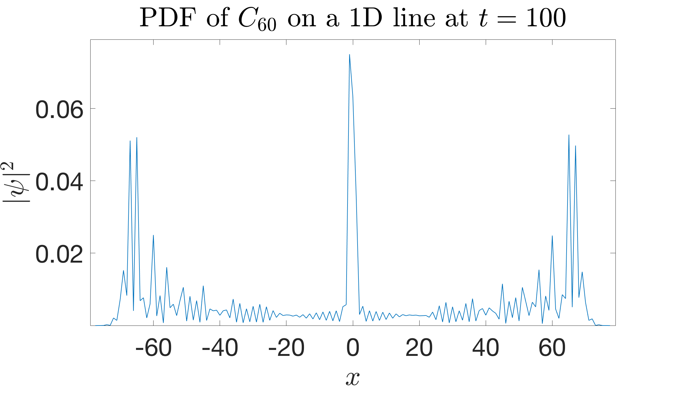
Figure 1: Snapshot of the probability density function $\rho\left(x,t\right)=\left|\psi_{x,t}^{2}\right|$ after $t=100$ updates using ${\cal C}_{60}$ in Eq. (8) for a quantum walk starting from the origin. As for the equivalent walk with the Grover coin in Eq. (7), see Refs. Inui et al. (2005); Falkner and Boettcher (2014), this walk exhibits a permanently localized component near its origin, while the remaining weight of the wave-function spreads ballistically in both directions along the lattice.

Such a 3-state quantum walk on the 1d-line has been investigated previously for a $3\times 3$ Grover coin Inui et al. (2005); Falkner and Boettcher (2014),

$${\cal C}_{G}=\frac{1}{3}{\textstyle\left[\begin{array}[]{rrr}-1&2&2\\ 2&-1&2\\ 2&2&-1\end{array}\right]}.$$ (7)

While the 3-dimensional coin attains the same asymptotic scaling as the more widely studied 2-dimensional case, it adds the interesting new aspect of localization to the dynamics Inui et al. (2005); Falkner and Boettcher (2014), where the walker becomes eternally confined near its starting site with a finite probability. In the following, we will investigate the effects of a non-reflective coin,

$${\cal C}_{60}=\frac{1}{3}{\textstyle\left[\begin{array}[]{rrr}2&2&-1\\ -1&2&2\\ 2&-1&2\end{array}\right]}.$$ (8)

As the geometry is simple, it is not too surprising that we find qualitatively the same phenomenology for both coins, as shown in Fig. 1. Thus, we will not bother with the canonical Fourier solution of the problem that can be found elsewhere Inui et al. (2005); Falkner and Boettcher (2014). Instead, we will immediately proceed to treat this problem as an exactly solvable example for the RG from which we can glean insights on how to treat more complicated non-Grover quantum walks with RG.

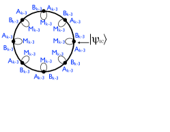
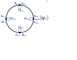
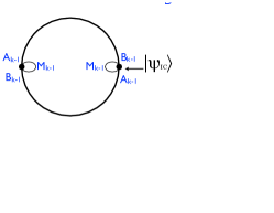
Figure 2: Depiction of the final three RG-steps for a simple 1d-line.

II.1 RG for the Quantum Walk on the Line

The transformed master equation (4) with ${\cal U}$ in Eq. (5) becomes $\overline{\psi}_{x}=zM\overline{\psi}_{x}+zA\overline{\psi}_{x-1}+zB\overline{\psi}_{x+1}$, which is the starting point for the RG. For simplicity, we consider the walk problem here with initial conditions (IC) localized at the origin, $\psi_{x,t=0}=\delta_{x,0}\psi_{IC}$. As depicted in Fig. 2, we recursively eliminate $\overline{\psi}_{x}$ for all sites for which $x$ is an odd number, then set $x\to x/2$ and repeat, step-by-step for $k=0,1,2,\ldots$. Starting at $k=0$ with the “raw” hopping coefficients $A_{0}=zA$, $B_{0}=zB$, and $M_{0}=zM$, after each step, the master equation becomes self-similar in form when redefining the renormalized hopping coefficients $A_{k}$, $B_{k}$, $M_{k}$. E.g., near any even site $x$ at step $k$ we have Boettcher et al. (2013):

$$\overline{\psi}_{x-1} = M_{k}\overline{\psi}_{x-1}+A_{k}\overline{\psi}_{x-2}+B_{k}\overline{\psi}_{x},$$

$$\overline{\psi}_{x} = M_{k}\overline{\psi}_{x}+A_{k}\overline{\psi}_{x-1}+B_{k}\overline{\psi}_{x+1}+\delta_{x,0}\psi_{IC},$$ (9)

$$\overline{\psi}_{x+1} = M_{k}\overline{\psi}_{x+1}+A_{k}\overline{\psi}_{x}+B_{k}\overline{\psi}_{x+2}.$$

Solving this linear system for site $x$ yields $\overline{\psi}_{x}=M_{k+1}\overline{\psi}_{x}+A_{k+1}\overline{\psi}_{x-2}+B_{k+1}\overline{\psi}_{x+2}$ with RG “flow”

$$A_{k+1} = A_{k}\left(\mathbb{I}-M_{k}\right)^{-1}A_{k},\qquad B_{k+1}=B_{k}\left(\mathbb{I}-M_{k}\right)^{-1}B_{k},$$ (10)

$$M_{k+1} = M_{k}+A_{k}\left(\mathbb{I}-M_{k}\right)^{-1}B_{k}+B_{k}\left(\mathbb{I}-M_{k}\right)^{-1}A_{k}.$$

II.2 RG-Analysis for the Grover Coin

For the quantum walk with the Grover coin ${\cal C}_{G}$ in Eq. (8), we evolve Eqs. (10) for a few iterations from its unrenormalized values Boettcher et al. (2013). Already after the first iteration, a recurring pattern emerges that suggest the Ansatz $A_{k}=a_{k}S^{A}{\cal C}_{G}$, $B_{k}=a_{k}S^{B}{\cal C}_{G}$, and

$$M_{k}=\left[\begin{array}[]{ccc}0&b_{k}&0\\ b_{k}&0&0\\ 0&0&z\end{array}\right]{\cal C}_{G},$$ (11)

where at $k=1$ the RG-flow gets initiated with

$$a_{k=1}=\frac{z^{2}\left(z-1\right)}{z+3}, b_{k=1}=\frac{2z^{2}\left(z+1\right)}{z+3}.$$ (12)

For this scalar parametrization with $a_{k}$ and $b_{k}$, the RG-flow (10) closes after each iteration for

$$a_{k+1} = \frac{a_{k}^{2}\left(z-1\right)}{\left(b_{k}-1\right)\left[\left(3z+1\right)b_{k}-z-3\right]},$$ (13)

$$b_{k+1} = b_{k}+\frac{a_{k}^{2}\left[\left(3z+1\right)b_{k}-2z-2\right]}{\left(b_{k}-1\right)\left[\left(3z+1\right)b_{k}-z-3\right]}$$

These recursions have a non-trivial fixed point at $\left(a_{\infty},b_{\infty}\right)=\left(\frac{1-z}{1+3z},\frac{2\left(1+z\right)}{1+3z}\right)$, yet, its Jacobian $J_{\infty}=\left.\frac{\partial\left(a_{k+1},b_{k+1}\right)}{\partial\left(a_{k},b_{k}\right)}\right|_{k\to\infty}$ is, in fact, $z$-independent and has a degenerate eigenvalue $\lambda_{1,2}=2$. Note that we never had to specify a choice for $z$ as the location of a fixed point to arrive at this result. However, numerical iteration of the RG-flow in Eq. (13) from the initial conditions in Eq. (12) clearly shows that fixed points are only attained for very specific choices of $z$. Those values of $z$ can be obtained by equating $\left(a_{\infty},b_{\infty}\right)=\left(a_{k},b_{k}\right)$, which provides an over-constraint condition on solving for $z$. For instance, the initial conditions in Eq. (12) merely yield $z=\pm 1$ as fixed points for $k=1$, $k=2$ adds $z=-\left(2\pm i\sqrt{5}\right)/3$, etc. We will return to this issue later.

Previously Boettcher et al. (2017), it was observed that is not sufficient to consider the hopping parameters $\left(a_{k},b_{k}\right)$ alone. To study the true scaling behavior, actual observables need to be examined; although observables are functionals of the hopping parameters, they are constrained to be unitary, unlike the hopping parameters. As in the classical analysis of a random walk Redner (2001), there is an intimate connection between fixed points and the poles in the complex-$z$ plane. The evolution under rescaling size ($k$) of those poles nearest to the fixed point yields the rescaling in time. While those poles move both radially as well as tangentially along the unit-circle for hopping parameters, they are constrained to moving only tangentially strictly on the circle for a unitary observable, leading to the walk dimension

$$d_{w}^{Q}=\log_{2}\sqrt{\lambda_{1}\lambda_{2}}.$$ (14)

Hence, with $\lambda_{1}=\lambda_{2}=2$, we obtain $d_{w}^{Q}=1$, as expected for a quantum walk on the 1d-line. We proceed to investigate such an observable more closely.

As shown in Fig. 2, the 1d-loop of $N=2^{k}$ sites after $k-1$ RG-steps reduces to merely two sites:

$$\overline{\psi}_{0} = M_{k-1}\overline{\psi}_{0}+\left(A_{k-1}+B_{k-1}\right)\overline{\psi}_{\frac{N}{2}}+\psi_{IC},$$

$$\overline{\psi}_{\frac{N}{2}} = M_{k-1}\overline{\psi}_{\frac{N}{2}}+\left(A_{k-1}+B_{k-1}\right)\overline{\psi}_{0}.$$ (15)

Eliminating also the site $\overline{\psi}_{\frac{N}{2}}$, and utilizing the RG-recursions in Eq. (10), we get the amplitude at the origin $x=0$ of a quantum walk, $\overline{\psi}_{0}=X_{k}\psi_{IC}$, for the 1d-line:

$$X_{k}=\left[\mathbb{I}-\left(A_{k}+B_{k}+M_{k}\right)\right]^{-1}.$$ (16)

It is now straightforward from the expressions near Eq. (11) to express the observable $X_{k}$ in terms of the hopping parameters $\left(a_{k},b_{k}\right)$:

$$X_{k}=\frac{\left[\begin{array}[]{ccc}\frac{-z-3+a_{k}\left(z-1\right)+2b_{k}\left(z+1\right)}{1+a_{k}-b_{k}}&\frac{-2a_{k}\left(z+1\right)-b_{k}\left(z-1\right)}{1+a_{k}-b_{k}}&-2a_{k}-2b_{k}\\ \frac{-2a_{k}\left(z+1\right)-b_{k}\left(z-1\right)}{1+a_{k}-b_{k}}&\frac{-z-3+a_{k}\left(z-1\right)+2b_{k}\left(z+1\right)}{1+a_{k}-b_{k}}&-2a_{k}-2b_{k}\\ -2z&-2z&a_{k}+b_{k}-3\end{array}\right]}{\left(a_{k}+b_{k}\right)\left(3z+1\right)-\left(z+3\right)}.$$ (17)

It is further fruitful to first solve the RG-flow in Eq. (13) in closed form. A simple rational Ansatz, amazingly, yields the exact solution

$$a_{k} = \frac{\left(u-1\right)\left(z-1\right)\left(3uz+u-z-3\right)\xi^{2^{k-1}}}{\left(z-1\right)^{2}-\left(3uz+u-2z-2\right)^{2}\xi^{2^{k}}},$$ (18)

$$b_{k} = \frac{u\left(z-1\right)^{2}-\left(3uz+u-2z-2\right)\left(2uz+2u-z-3\right)\xi^{2^{k}}}{\left(z-1\right)^{2}-\left(3uz+u-2z-2\right)^{2}\xi^{2^{k}}},$$

where the otherwise free constants $u$ and $\xi$ are fixed by the initial conditions at $k=1$ in Eq. (12):

$$\xi = 16+9\cos\left(2\omega\right)+24\cos\omega-\cos\frac{\omega}{2}\left(6\cos\omega+4\right)\sqrt{18\cos\omega+6},$$

$$u = e^{i\omega}\left[\frac{3}{2}\cos\omega-\frac{1}{2}+\frac{1}{2}\cos\frac{\omega}{2}\sqrt{18\cos\omega+6}\right],$$ (19)

using $z=e^{i\omega}$. Note that $\xi$ is complex (with $\left|\xi\right|=1$) only for $\omega=\arg z\in I$ on the interval $I=\left(\pi-\arctan 2\sqrt{2},\pi+\arctan 2\sqrt{2}\right)$. An infinity of solutions for $\omega$ of $\xi^{2^{j}}=1$ for any integer $j\geq 0$ form a (likely dense) set of fixed points of the RG-flow on $I$, because they leave Eq. (18) invariant for all $j\leq k\leq\infty$.

It is instructive to define $\xi=e^{i\nu}$ and $u=\left[2\left(z+1\right)+ie^{i\sigma}\left(z-1\right)\right]/\left(3z+1\right)$ to get

$$\cos\nu = 9\cos\left(2\omega\right)+24\cos\left(\omega\right)+16,$$

$$\sin\sigma = -\frac{9}{4}z^{2}-\frac{3}{2}z-\frac{5}{4}.$$ (20)

Then, the solution of the RG-flow given in Eq. (18) simplifies to

$$a_{k} = \frac{\left(1-z\right)\cos\sigma}{\left(3z+1\right)\cos\left(2^{k}\nu+\sigma\right)},$$ (21)

$$b_{k} = \frac{2\left(z+1\right)}{3z+1}+\frac{\left(z-1\right)\sin\left(2^{k}\nu\right)}{\left(3z+1\right)\cos\left(2^{k}\nu+\sigma\right)}.$$

From Eq. (17) we thus find

$$X_{k} = \frac{\chi}{\left(z-1\right)\sin\left(2^{k-1}\nu\right)},$$ (22)

with a regular numerator matrix $\chi$ that does not have any $k$-dependent poles.

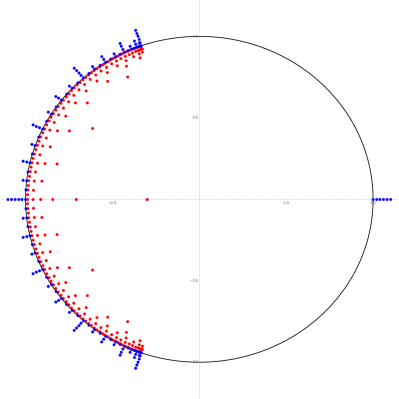
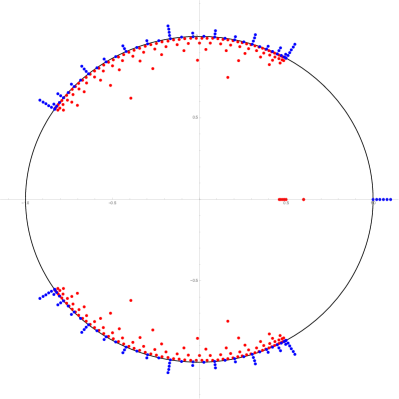
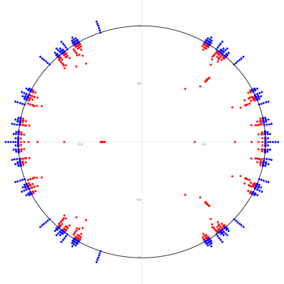
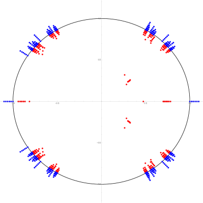
Figure 3: Plot of the poles of the Laplace transforms in the complex-$z$ plane for the hopping parameters $a_{k}$ and $b_{k}$ (red points), and for the amplitude to remain at the origin, $\overline{\psi}_{0}^{(k)}(z)=X_{k}\psi_{IC}$ (blue points). Shown are the poles for the first few consecutive RG-steps ($k=1,\ldots,6$) for a quantum walk on the 1$d$-line (top) and DSG (bottom). On the left, the quantum walk is driven by the Grover coin in Eq. (7), and on the right, the rotational coin in Eq. (8) was applied. Since both coins are real, poles are certain to occur in complex-conjugate pairs. As $X_{k}$ is unitary, all its poles are on the unit-circle (black line) in the complex-$z$ plane, however, for better visibility we have offset poles increasingly outward for smaller $k$. Since the poles of the hopping parameters are all strictly outside (but converging onto) the unit-circle, we have applied the same offset but also mapped the poles (by $z\to 1/z$) to the inside. Note that if a pole for the observable arises at some $k_{0}$, it remains to be a pole for all $k\geq k_{0}$; this is not true for the hopping parameters. Generally, the pattern by which poles evolve appears more complicated for DSG. For walks with the Grover coin ${\cal C}_{G}$, ever more poles progressively impinge on the real-$z$ axis, at either of $z=\pm 1$, or both. For the non-reflective coin ${\cal C}_{60}$, the accumulation points for poles generally reside at non-trivial locations , for example at $\arg z=\pi\pm\arctan\sqrt{35}$ for the 1$d$-line (top-right). Typically, the edges of the wedges within which poles accumulate represent fixed points that yield exponents for the classical random walk, such as at $\arg z=\pi\pm\arctan 2\sqrt{2}$ for the 1$d$-line with Grover coin (top-left), or at both, $\arg z=\pi\pm\arctan\frac{\sqrt{11}}{5}$ and $\arg z=\pm\frac{\pi}{3}$, for the 1$d$-line with the non-reflective coin (top-right). The domains in which poles appear to become dense seem to break up like fractal Kantor-sets for the DSG.

Note that the observable $X_{k}$ in Eq. (22) has poles for $z=1$ and for real $\nu_{n}^{(k)}=n\pi/2^{k-1}$, $0\leq n<2^{k}$. By Eq. (20), however, $\nu$ can be real only for real $\omega=\arg z\in I$, i.e., on the corresponding segment of the unit-circle in the complex-$z$ plane (where we furthermore have a uni-modular $\xi=e^{i\nu}$, $\left|\xi\right|=1$). The corresponding values for $\omega_{n}^{(k)}$ can be obtained from Eq. (20). Those Laplace-poles $\omega_{n}^{(k)}$ are shown in Fig. 3, obtained directly by iteration of the RG-flow for $k=1,\ldots,6$. The corresponding poles for the hopping parameters in Eq. (21) are at $\nu_{m}^{(k)}=(m\pi+1/2-\sigma)/2^{k-1}$, $0\leq m<2^{k}$, pushed slightly off the unit-circle by $\sigma$, as is generally the case Boettcher et al. (2017). There is clearly a connection between those poles and the aforementioned fixed points, as $2^{k}\nu_{n}^{(j)}$ for $k\geq j$ is always an integer multiple of $2\pi$, such that the corresponding $\omega_{n}^{(j)}$ is also always a fixed point in Eq. (21). Thus, expanding an observable like $X_{k}$ for large $k$ (i.e., for any fixed point $\omega_{n}^{(j)}$ it is assumed $k\gg j$) implies an expansion around such a pole, and one generically finds

$$X_{k} \sim\sum_{l=-1}^{\infty} {\cal M}_{l}\,\left(N\zeta\right)^{l},\qquad\left(\zeta=z-z_{{\rm FP}}\to 0\right),$$ (23)

where we set $z_{{\rm FP}}=e^{i\omega_{n}^{(j)}}$, and all ${\cal M}_{l}\left(z_{{\rm FP}}\right)$ are matrices that become constant after neglecting higher-order corrections in inverse size $N=2^{k}$ for each order in $\zeta$. Although those constants vary with the choice of $z_{{\rm FP}}$, they can not affect the sought-after scaling behavior. Clearly, $z_{{\rm FP}}=-1$ is the most convenient (and symmetric, see Fig. 3) choice. The classical choice $z_{{\rm FP}}=1$ would not work, even though $z=1$ is a pole of $X_{k}$. However, that pole is isolated, as Fig. 3 shows, and we observe from Eq. (21) that $\left(a_{k},b_{k}\right)=\left(0,1\right)$ is trivial and without $N$-dependence in its expansion.

Finally, we study how these choices affect the asymptotic analysis of the RG-flow in Eq. (13). After all, and as we will see below, we are typically not in possession of the exact location of poles. In some elementary case, like the 2-state quantum walk on a line Boettcher and Li (4692), the RG-flow does not have an explicit $z$-dependence and the expansion around some $z_{{\rm FP}}$ remains purely formal, without any need for specificity. Even if $z$ explicitly appears, such as in Eq. (13), we can replace $z=z_{{\rm FP}}+\left(z-z_{{\rm FP}}\right)\sim z_{{\rm FP}}$, since we are aiming to analyze an unstable fixed point with diverging corrections, which corrections in small $\left(z-z_{{\rm FP}}\right)$ can not provide. To wit, for a generic RG-flow $\vec{a}_{k+1}(z)={\cal RG}\left(\vec{a}_{k}(z);z\right)$, expanded around the fixed point $z_{{\rm FP}}$ in the limit of large system sizes, $k\to\infty$, we have to linear order:

$$\vec{\alpha}_{k+1}(z) \sim \left[\vec{\alpha}_{k}\circ\vec{\nabla}_{\vec{a}}+\left(z-z_{{\rm FP}}\right)\partial_{z}\right]{\cal RG}\left(\vec{a}_{\infty}(z_{{\rm FP}});z_{{\rm FP}}\right)+\ldots,$$ (24)

with $\vec{\alpha}_{k}(z)=\vec{a}_{k}(z)-\vec{a}_{\infty}(z_{{\rm FP}})$ with $\vec{a}_{\infty}(z_{{\rm FP}})={\cal RG}\left(\vec{a}_{\infty}(z_{{\rm FP}});z_{{\rm FP}}\right)$ defining the fixed point. It is then the divergent eigen-solutions $\left\{\lambda_{i},\vec{v}_{i}\right\}$ of the Jacobian $J_{\infty}=\vec{\nabla}_{\vec{a}}{\cal RG}\left(\vec{a}_{\infty}(z_{{\rm FP}});z_{{\rm FP}}\right)$, i.e., those with eigenvalues $\lambda_{i}>1$, that dominate the solution for $k\to\infty$, while the $k$-independent inhomogeneity $\left(z-z_{{\rm FP}}\right)\partial_{z}{\cal RG}\left(\vec{a}_{\infty}(z_{{\rm FP}});z_{{\rm FP}}\right)$ remains irrelevant, to this and also in higher orders:

$$\vec{\alpha}_{k}(z) \sim{\cal A}\lambda_{1}^{k}\vec{v}_{1}+{\cal B}\lambda_{2}^{k}\vec{v}_{2}+\ldots$$ . (25)

In the case at hand in Eq. (13), we find that the Jacobian is already diagonal such that the eigenvectors are elementary, $\vec{v}_{i}=\widehat{e}_{i}$, with divergent eigenvectors $\lambda_{1}^{k}=\lambda_{2}^{k}=2^{k}=N$, and we can insert:

$$a_{k}\left(z\right) \sim a_{\infty}+\zeta{\cal A}\lambda_{1}^{k}+\zeta^{2}\alpha_{k}^{(2)}+\zeta^{3}\alpha_{k}^{(3)}+\ldots,$$

$$b_{k}\left(z\right) \sim b_{\infty}+\zeta{\cal B}\lambda_{2}^{k}+\zeta^{2}\beta_{k}^{(2)}+\zeta^{3}\beta_{k}^{(3)}+\ldots,$$ (26)

while simply setting $z=z_{{\rm FP}}$. We then find as the most-divergent terms in each order:

$$\alpha_{k}^{(2)} \sim \frac{1+3z_{{\rm FP}}}{2\left(1-z_{{\rm FP}}\right)}\left[\left({\cal A}\lambda_{1}^{k}\right)^{2}+\left({\cal B}\lambda_{2}^{k}\right)^{2}\right]+\ldots,$$

$$\alpha_{k}^{(3)} \sim \frac{\left(1+3z_{{\rm FP}}\right)^{2}}{6\left(1-z_{{\rm FP}}\right)^{2}}\left[\left({\cal A}\lambda_{1}^{k}\right)^{3}+5\left({\cal A}\lambda_{1}^{k}\right)\left({\cal B}\lambda_{2}^{k}\right)^{2}\right]+\ldots,$$

$$\beta_{k}^{(2)} \sim \frac{1+3z_{{\rm FP}}}{2\left(1-z_{{\rm FP}}\right)}\left({\cal A}\lambda_{1}^{k}\right)\left({\cal B}\lambda_{2}^{k}\right)+\ldots,$$ (27)

$$\beta_{k}^{(3)} \sim \frac{\left(1+3z_{{\rm FP}}\right)^{2}}{3\left(1-z_{{\rm FP}}\right)^{2}}\left[2\left({\cal A}\lambda_{1}^{k}\right)^{2}\left({\cal B}\lambda_{2}^{k}\right)+\left({\cal B}\lambda_{2}^{k}\right)^{3}\right]+\ldots.$$

Inserted into $X_{k}$ in Eq. (17), we indeed faithfully reproduce the expansion in Eq. (23), up to unknown (and irrelevant) constants. Not surprisingly, we find that the choice of $z_{{\rm FP}}$ does not affect the scaling results, except that $z_{{\rm FP}}=1$ is excluded, consistent with the direct expansion of the exact solution.

II.3 RG-Analysis for the Non-reflective Coin

We apply the same strategy for the quantum walk with the non-reflective coin ${\cal C}_{60}$ in Eq. (7): evolving Eqs. (10) for a few iterations from its unrenormalized values Boettcher et al. (2013), a recurring pattern emerges that suggests again the Ansatz $A_{k}=a_{k}S^{A}{\cal C}_{60}$, $B_{k}=a_{k}S^{B}{\cal C}_{60}$, and

$$M_{k}=m_{k}\left[\begin{array}[]{ccc}0&\left(\frac{2-z}{2z-1}\right)b_{k}&0\\ b_{k}&0&0\\ 0&0&z\end{array}\right]{\cal C}_{60}.$$ (28)

Starting from

$$a_{k=1}=\frac{2z^{2}\left(z-1\right)}{2z-3},\qquad b_{k=1}=\frac{z^{2}\left(1-2z\right)}{2z-3},\\$$ (29)

the RG-flow now closes after each iteration for

$$a_{k+1} = \frac{2\left(z-1\right)\left(2z-1\right)a_{k}^{2}}{(2z-3)(2z-1)-2(z-2)(2z-1)b_{k}+(z-2)(3z-2)b_{k}^{2}},$$ (30)

$$b_{k+1} = b_{k}+\frac{2\left(2z-1\right)a_{k}^{2}\left[\left(3z-2\right)b_{k}-2z+1\right]}{(2z-3)(2z-1)-2(z-2)(2z-1)b_{k}+(z-2)(3z-2)b_{k}^{2}}.$$

Again, there is a close-form solution for the RG-flow:

$$a_{k} = \frac{2\left(z-1\right)\left[\left(z-2\right)\left(3z-2\right)u^{2}-2\left(z-2\right)\left(2z-1\right)u+4z^{2}-8z+3\right]\xi^{2^{k-1}}}{4\left(2z-1\right)\left(z-1\right)^{2}+\left(z-2\right)\left[\left(3z-2\right)u-2z+1\right]^{2}\xi^{2^{k}}},$$

$$b_{k} = \frac{2\left(z-1\right)\left\{4\left(z-1\right)^{2}u+\left[\left(z-2\right)u-2z+3\right]\left[\left(3z-2\right)u-2z+1\right]\xi^{2^{k}}\right\}}{4\left(2z-1\right)\left(z-1\right)^{2}+\left(z-2\right)\left[\left(3z-2\right)u-2z+1\right]^{2}\xi^{2^{k}}},$$ (31)

where from Eq. (29) at $k=1$ we get with $z=e^{i\omega}$:

$$\xi = \frac{11}{8}+\frac{3}{2}\cos\omega+\frac{9}{4}\cos 2\omega-\frac{\sqrt{3}}{8}\left(1+6\cos\omega\right)\sqrt{1+4\cos\omega+6\cos 2\omega},$$

$$u = e^{i\omega}\frac{2\cos\frac{\omega}{2}-3\cos\frac{3\omega}{2}-i\sqrt{3}\sin\frac{\omega}{2}\sqrt{1+4\cos\omega+6\cos 2\omega}}{4\cos\omega-5}.$$ (32)

In correspondence with Eq. (19), we note that $\xi$ here is complex (with $\left|\xi\right|=1$) for $\omega=\arg z\in I_{\pm}$ on the conjugate intervals $I_{\pm}=\left(\pm\frac{\pi}{3},\pi\mp\arctan\frac{\sqrt{11}}{5}\right)$, leading to an infinity of solutions for $\omega$ of $\xi^{2^{j}}=1$ for any integer $j\geq 0$ form a (likely dense) set of fixed points of the RG-flow on $I_{\pm}$, because they leave Eq. (31) invariant for all $j\leq k\leq\infty$. As in the previous case for a Grover coin, Laplace poles of observables will be found to cluster on these intervals of the unit-circle in the complex-$z$ plane, see Fig. 3. Most remarkable here is the fact that the real axes, i.e., $z=\pm 1$, are not inside those intervals. Extending this analysis to a new set of variables, $\xi=e^{i\nu}$ and $u=\frac{2\left(z-1\right)}{2-3z}\sqrt{\frac{2z-1}{z-2}}e^{i\sigma}+\frac{2z-1}{3z-2}$, we find in analogy to Eq. (20):

$$\cos\nu=\frac{11}{8}+\frac{3}{2}\cos\omega+\frac{9}{4}\cos 2\omega,\qquad\sin\sigma=\frac{9z^{3}-3z^{2}-z+2}{4\sqrt{\left(2z-1\right)\left(2-z\right)}}.$$ (33)

In terms of these variables, we can conveniently express the solutions in Eq. (30) as

$$a_{k} = \frac{2\left(z-1\right)\cos\sigma}{\left(3z-2\right)\cos\left(2^{k}\nu+\sigma\right)},$$ (34)

$$b_{k} = \frac{2z-1}{3z-2}+\frac{2\left(z-1\right)\sqrt{2z-1}\sin\left(2^{k}\nu\right)}{\left(3z-2\right)\sqrt{2-z}\cos\left(2^{k}\nu+\sigma\right)}.$$

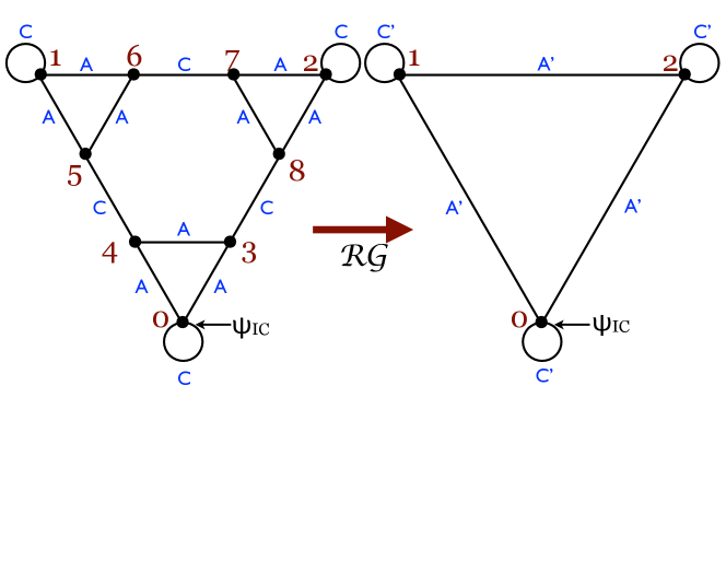
Figure 4: Depiction of the (final) RG-step in the analysis of DSG. The letters $\left\{A,C\right\}$ label transitions between sites (black dots on the vertices) of the quantum walk in the form of hopping matrices. (Only on the three outermost sites, the matrix $C$ refers back to the same site. For simplicity, we have omitted all such self-loops associated with hopping matrix $M$ at each site.) Recursively, the inner-6 sites (labeled $3,\ldots,8$) of each larger triangle (left) in DSG are decimated to obtain a reduced triangle (right) with renormalized hopping matrices (primed). To build a DSG of $N=3^{g}$ sites, this procedure is applied (in reverse) $g$ times to all triangles at each generation. Note that each generation the base-length $L$ increases by a factor of $b=2$, such that the fractal dimension is $d_{f}=\log_{b=2}3$.

Using Eq. (16), we obtain the observable $X_{k}$, which in terms of Eq. (34) takes on the same form as in Eq. (22) (with an equivalent but numerically different matrix $\chi$). All of $a_{k}$, $b_{k}$, and $X_{k}$ appear very similar to their counterparts derived from the Grover coin in Sec. II.2, with poles of $X_{k}$ for $z=1$ and for real $\nu_{n}^{(k)}=n\pi/2^{k-1}$, $0\leq n<2^{k}$. In terms of the location of the poles in the complex-$z$ plane these values are attained via $\cos\nu$ as given in Eqs. (20) and (33), respectively. Accordingly, the $\nu_{n}^{(k)}$ get mapped onto the unit-circle with $\omega=\arg z$ in the intervals $I$ and $I_{\pm}$, respectively, as shown in Fig. 3, knowledge of which would be essential to expand the exact $X_{k}$ around some pole within the respective intervals. In contrast, the expansion of the RG-flow around some putative fixed point $z_{{\rm FP}}$, for either the non-reflective coin just or for the Grover coin in Eq. (26), is oblivious to the choice of $z_{{\rm FP}}$ in so far as the sought-after scaling behavior is concerned [i.e., aside from any numerical factors dependent on $z_{{\rm FP}}$, as in Eq. (27)]. However, exceptional points may exist, such as the isolated pole at $z=1$ in both examples, that should be avoided.

Despite the similarities in the analysis in both cases, the shift in poles away from the real-$z$ axis could have signaled a change in universality classes for the quantum walk with these very distinct coins. Yet, in this simple example of a 1d-walk, we find that both RG-flows provide identical eigenvalues for their Jacobians, leaving the walk dimension $d_{w}^{Q}$ in Eq. (14) unchanged. In the following, we will apply these insights to the more involved (and not exactly solvable) RG-flow for a quantum walk on a dual Sierpinski gasket (DSG).

III Quantum Walk on the Dual Sierpinski Gasket

Basically, the same procedure as in Sec. II.1, although algebraically more laborious, can be applied to obtain closed RG-recursions for a number of fractal networks Boettcher et al. (2014, 2015). These have provided the first exact weak-limit results Grimmett et al. (2004); Konno (2005); Falkner and Boettcher (2014) for non-trivial networks beyond regular lattices.

Due to the self-similarity of fractal networks, we can decompose ${\cal U}_{x,y}$ in Eq. (4) into its smallest sub-structure, exemplified by Fig. 4. It shows the elementary graph-let of nine sites that is used to recursively build the dual Sierpinski gasket (DSG) of size $N=3^{g}$ after $g$ generations. The master equations pertaining to these sites are:

$$\overline{\psi}_{0} = \left(M+C\right)\overline{\psi}_{0}+A\left(\overline{\psi}_{3}+\overline{\psi}_{4}\right)+\psi_{IC},$$

$$\overline{\psi}_{\left\{1,2\right\}} = \left(M+C\right)\overline{\psi}_{\left\{1,2\right\}}+A\left(\overline{\psi}_{\left\{5,7\right\}}+\overline{\psi}_{\left\{6,8\right\}}\right),$$ (35)

$$\overline{\psi}_{\left\{3,4,5,6,7,8\right\}} = M\overline{\psi}_{\left\{3,4,5,6,7,8\right\}}+C\overline{\psi}_{\left\{8,5,4,7,6,3\right\}}+A\left(\overline{\psi}_{\left\{0,3,1,5,2,7\right\}}+\overline{\psi}_{\left\{4,0,6,1,8,2\right\}}\right).$$

The hopping matrices $A$ and $C$ describe transitions between neighboring sites, while $M$ permits the walker to remain on its site in a “lazy” walk. The inhomogeneous $\psi_{IC}$-term allows for an initial condition $\psi_{x,t=0}=\delta_{x,0}\psi_{IC}$ for a quantum walker to start at site $x=0$ in state $\psi_{IC}$.

III.1 Renormalization Group

To accomplish the decimation of the sites $\overline{\psi}_{\left\{3,\ldots,8\right\}}$, as indicated in Fig. 4, we need to solve the linear system in Eqs. (35) for $\overline{\psi}_{\left\{0,1,2\right\}}$. Thus, we expect that $\overline{\psi}_{\left\{3,\ldots,8\right\}}$ can be expressed as (symmetrized) linear combinations

$$\overline{\psi}_{\left\{3,4\right\}} = P\overline{\psi}_{0}+Q\overline{\psi}_{\left\{1,2\right\}}+R\overline{\psi}_{\left\{2,1\right\}},$$

$$\overline{\psi}_{\left\{5,8\right\}} = R\overline{\psi}_{0}+P\overline{\psi}_{\left\{1,2\right\}}+Q\overline{\psi}_{\left\{2,1\right\}},$$ (36)

$$\overline{\psi}_{\left\{6,7\right\}} = Q\overline{\psi}_{0}+P\overline{\psi}_{\left\{1,2\right\}}+R\overline{\psi}_{\left\{2,1\right\}}.$$

Inserting this Ansatz into Eqs. (35) and comparing coefficients provides consistently for the unknown matrices:

$$P = \left(M+A\right)P+A+CR,$$

$$Q = \left(M+C\right)Q+AR,$$ (37)

$$R = MR+AQ+CP.$$

Using the abbreviations $S=\left(\mathbb{I}-M-C\right)^{-1}A$ and $T=\left(\mathbb{I}-M-AS\right)^{-1}C$, Eqs. (37) have the solution:

$$P=\left(\mathbb{I}-M-A-CT\right)^{-1}A,\qquad R=TP,\qquad Q=SR.$$ (38)

Finally, after $\overline{\psi}_{\left\{3,\ldots,8\right\}}$ have been eliminated, we find

$$\overline{\psi}_{0} =\left(\left[M+2AP\right]+C\right)\overline{\psi}_{0}+A\left(Q+R\right)\left(\overline{\psi}_{1}+\overline{\psi}_{2}\right)+\psi_{IC},$$ (39)

$$\overline{\psi}_{\left\{1,2\right\}} =\left(\left[M+2AP\right]+C\right)\overline{\psi}_{\left\{1,2\right\}}+A\left(Q+R\right)\left(\overline{\psi}_{0}+\overline{\psi}_{\left\{2,1\right\}}\right).$$

By comparing coefficients between the renormalized expression in Eq. (39) and the corresponding, self-similar expression in the first line of Eqs. (35), we can identify the RG-recursions

$$M_{k+1} = M_{k}+2A_{k}P_{k},$$

$$A_{k+1} = A_{k}\left(Q_{k}+R_{k}\right),$$

$$C_{k+1} = C_{k},$$ (40)

where the subscripts refer to $k$- and $(k+1)$-renormalized forms of the hopping matrices. These recursions evolve from the un-renormalized ($k=0$) hopping matrices with $\left\{M,A,C\right\}_{k=0}=z\left\{M,A,C\right\}$. These RG-recursions are entirely generic and, in fact, would hold for any walk on DSG, classical or quantum. In the following, we now consider a specific form of a quantum walk with both, the Grover coin in Eq. (7) as well as the non-reflective coin in Eq. (8).

As an observable, we focus again on $\overline{\psi}_{0}(z)$, the amplitude at the origin of the quantum walk on DSG, here chosen on one of the corner-sites. According to Fig. 4 and Eq. (39), we have

$$\overline{\psi}_{0} = \left(M_{k}+C_{k}\right)\overline{\psi}_{0}+A_{k}\left(\overline{\psi}_{1}+\overline{\psi}_{2}\right)+\psi_{IC},$$ (41)

$$\overline{\psi}_{\left\{1,2\right\}} = \left(M_{k}+C_{k}\right)\overline{\psi}_{\left\{1,2\right\}}+A_{k}\left(\overline{\psi}_{0}+\overline{\psi}_{\left\{2,1\right\}}\right),$$

which has the solution $\overline{\psi}_{0}=X_{k}\psi_{IC}$ with

$$X_{k}=\left[\mathbb{I}-M_{k}-C_{k}-2A_{k}\left(\mathbb{I}-M_{k}-A_{k}-C_{k}\right)^{-1}A_{k}\right]^{-1}.$$ (42)

Preserving the norm of the quantum walk demands unitary propagation, i.e., $\mathbb{I}={\cal U}^{\dagger}{\cal U}$. In Ref. Boettcher et al. (5339), we have obtained generalized unitarity conditions for DSG as shown in Fig. 4:

$$\mathbb{I} = 2A^{\dagger}A+C^{\dagger}C+M^{\dagger}M,$$ (43)

$$0 = A^{\dagger}A+A^{\dagger}M+M^{\dagger}A=C^{\dagger}M+M^{\dagger}C=A^{\dagger}C.$$

III.2 RG-Analysis for the Quantum Walk with Grover Coin

In this section, we review the behavior of a coined quantum walk on the DSG with the Grover-coin ${\cal C}_{G}$ in Eq. (7), adapting the analysis from Ref. Boettcher and Li (4692). To study the scaling solution for the spreading quantum walk according to Eq. (1), as expressed by the walk dimension in Eq. (14), it is sufficient to investigate the properties of the RG-recursion in the previous section for $\left\{M,A,C\right\}$. In the unrenormalized (“raw”) description of the walk, these hopping matrices are chosen as

$$M=\left[\begin{array}[]{ccc}-\frac{1}{3}&0&0\\ 0&-\frac{1}{3}&0\\ 0&0&0\end{array}\right]{\cal C}_{G}, \quad A=\left[\begin{array}[]{ccc}\frac{2}{3}&0&0\\ 0&\frac{2}{3}&0\\ 0&0&0\end{array}\right]{\cal C}_{G},\quad C=\left[\begin{array}[]{ccc}0&0&0\\ 0&0&0\\ 0&0&1\end{array}\right]{\cal C}_{G}.$$ (53)

Here, we have to pay a small price for the fact that throughout, $A$ shifts weights symmetrically to two neighboring sites within their local triangle. To maintain the unitarity conditions in Eq. (43), the walk now must have a “lazy” component, i.e., some weight may remain at each site every update, so that $M\not=0$. The matrix $C$ shifts weight to the one neighbor outside those triangles, as illustrated in Fig. 4. These weights are the three complex components of the state vector at each site, $\psi_{x,t}$, which are all zero at $t=0$, except for $x=0$ where $\psi_{0,0}=\psi_{IC}$ is arbitrary but normalized, $\left|\psi_{IC}^{2}\right|=1$. These weights are mixed via ${\cal C}_{G}$ at each site before a shift entangles them within the network.

Iterating the RG-recursions in Eq. (40) for the matrices in Eq. (53) for only $k=2$ steps already reveals a simple recursive pattern that suggests the Ansatz

$$M_{k}=\left[\begin{array}[]{ccc}\frac{a_{k}-2b_{k}}{3}&\frac{a_{k}-2b_{k}}{3}+\frac{3z+1}{3/z+1}&0\\ \frac{a_{k}-2b_{k}}{3}+\frac{3z+1}{3/z+1}&\frac{a_{k}-2b_{k}}{3}&0\\ 0&0&0\end{array}\right]{\cal C}_{G},\quad A_{k}=\left[\begin{array}[]{ccc}\frac{a_{k}+b_{k}}{3}&\frac{a_{k}+b_{k}}{3}&0\\ \frac{a_{k}+b_{k}}{3}&\frac{a_{k}+b_{k}}{3}&0\\ 0&0&0\end{array}\right]{\cal C}_{G},$$ (60)

while $C_{k}=C_{0}=zC$ does not renormalize. Inserted into the RG-recursions in Sec. III.1, these matrices exactly reproduce themselves in form after one iteration, $k\to k+1$, when we identify for the scalar RG-flow:

$$a_{k+1} = \frac{\left(9z^{3}+5z^{2}-5z-9\right)\left(a_{k}-2b_{k}\right)-6\left(3z^{2}+10z+3\right)a_{k}b_{k}}{3\left(9z^{3}+5z^{2}-5z-9\right)+2\left(3z^{2}+10z+3\right)\left(2a_{k}-b_{k}\right)},$$

$$b_{k+1} = \frac{\begin{array}[]{l}4(3+z)\left(9-4z-14z^{2}+6z^{3}+27z^{4}\right)\left(2a_{k}-b_{k}\right)b_{k}-12(3+z)^{2}\left(9z^{2}-1\right)a_{k}b_{k}^{2}\\ \quad-\left(z^{2}-1\right)\left(9-10z+9z^{2}\right)\left(9+14z+9z^{2}\right)\left(a_{k}-2b_{k}\right)-24z(3+z)^{2}b_{k}^{2}\end{array}}{\begin{array}[]{l}4(3+z)\left(9-10z-16z^{2}+6z^{3}+27z^{4}\right)a_{k}+3\left(z^{2}-1\right)\left(9-10z+9z^{2}\right)\left(9+14z+9z^{2}\right)\\ \quad-8(3+z)\left(9+8z-10z^{2}+6z^{3}+27z^{4}\right)b_{k}-4(3+z)^{2}\left(9z^{2}-1\right)\left(2a_{k}-b_{k}\right)b_{k}\end{array}}.$$ (66)

This flow is initiated at $k=1$ with

$$a_{k=1}=\frac{z(z-1)\left(9+22z+9z^{2}\right)}{(3+z)\left(9+2z-3z^{2}\right)},\qquad b_{k=1}=\frac{z(1+z)\left(9+4z+6z^{2}+4z^{3}+9z^{4}\right)}{(3+z)\left(9+2z+4z^{2}-2z^{3}+3z^{4}\right)}.\\$$ (67)

Inserting Eq. (60) into Eq. (42), we then also have an expression for the observable $X_{k}$ in terms of the hopping parameters $a_{k}$ and $b_{k}$. Here, of course, we don’t have any closed-form solution of the RG-flow in Eq. (LABEL:eq:RGflowDSG). We can merely verify numerically with a few iterations of the RG-flow that the Laplace-poles of the hopping parameters as well as of the observable behave quite similarly as those for the Grover-coin walk on the 1d-line, see Fig. 3. Thus, in the case of the DSG, we only have the RG to rely on.

III.2.1 Fixed-Point Analysis

We now proceed to study the fixed-point properties of the RG-flow at $k\sim k+1\to\infty$. Eq. (LABEL:eq:RGflowDSG) has a non-trivial fixed point for $a_{\infty}\left(z\right)=\frac{\left(1-z\right)\left(9+14z+9z^{2}\right)}{2\left(z+3\right)\left(3z-1\right)}$ and $b_{\infty}(z)=\frac{\left(1+z\right)\left(9-10z+9z^{2}\right)}{2\left(z+3\right)\left(3z-1\right)}$. Due to the choice of $a_{k}$ and $b_{k}$ in Eq. (60), the Jacobian matrix $J_{\infty}=\left.\frac{\partial\left(a_{k+1},b_{k+1}\right)}{\partial\left(a_{k},b_{k}\right)}\right|_{k\to\infty}$ of the fixed point is already diagonal and $z$-independent, with two eigenvalues, $\lambda_{1}=3$ and $\lambda_{2}=\frac{5}{3}$, reproducing via Eq. (14) the already known result for the quantum walk dimension of the DSG with a Grover coin, $d_{w}^{Q}=\log_{2}\sqrt{5}$  Boettcher et al. (2015). Extending the expansion of Eq. (LABEL:eq:RGflowDSG) in powers of $\zeta=z-z_{{\rm FP}}$ for some unspecified fixed-point value $z_{{\rm FP}}$ for $k\to\infty$ to higher order, we obtain:

$$a_{k}\left(z\right) \sim a_{\infty}\left(z_{{\rm FP}}\right)+\zeta^{1}{\cal A}\lambda_{1}^{k}+\zeta^{2}\alpha_{k}^{(2)}+\zeta^{3}\alpha_{k}^{(3)}+\ldots,$$

$$b_{k}\left(z\right) \sim b_{\infty}\left(z_{{\rm FP}}\right)+\zeta^{1}{\cal B}\lambda_{2}^{k}+\ldots,$$ (68)

with unknown constants ${\cal A}$ and ${\cal B}$, and with

$$\alpha_{k}^{(2)} \sim c\left({\cal A}\lambda_{1}^{k}\right)^{2}+\ldots,$$ (69)

$$\alpha_{k}^{(3)} \sim c^{2}\left[\left({\cal A}\lambda_{1}^{k}\right)^{3}-\frac{1}{2}\left({\cal A}\lambda_{1}^{k}\right)^{2}\left({\cal B}\lambda_{2}^{k}\right)\right]+\ldots,$$

with $c=\left(9z_{{\rm FP}}^{2}-1\right)/\left(8z_{{\rm FP}}\right)$, where we have only kept leading-order terms in $k$ that contribute to leading order in large $k$. Note that $z_{{\rm FP}}$ has no effect on the scaling and merely contributes numerically for any choice of $z_{{\rm FP}}$ on the unit-circle, irrespective of the location of any poles. Inserting Eqs. (60) and (68) into $X_{k}$ in Eq. (42) and expanding (some generic component of $X_{k}$) in powers of $\zeta=z-z_{{\rm FP}}$ yields

$$\left[X_{k}\right]_{11} \sim -\zeta^{-1}\frac{z_{{\rm FP}}+3}{12\left(3z_{{\rm FP}}+1\right)\left({\cal A}\lambda_{1}^{k}\right)}-\zeta^{0}\left[\frac{\left(z_{{\rm FP}}+3\right)\left(3-25z_{{\rm FP}}-3z_{{\rm FP}}^{2}+9z_{{\rm FP}}^{3}\right)}{96z_{{\rm FP}}\left(z_{{\rm FP}}^{2}-1\right)}\right]$$

$$-\zeta^{1}\left[\frac{5\left(z_{{\rm FP}}+3\right)\left(3z_{{\rm FP}}-1\right)^{2}\left(3z_{{\rm FP}}+1\right)}{1536z_{{\rm FP}}^{2}}\left({\cal B}\lambda_{2}^{k}\right)\right]+\ldots,$$

$$\sim \zeta^{-1}O\left(\frac{1}{\lambda_{1}^{k}}\right)+\zeta^{0}O(1)+\zeta^{1}O\left(\lambda_{2}^{k}\right)+\ldots.$$

While this result reproduces those from Ref. Boettcher and Li (4692), it is remarkable that in this case we have to exclude the values $z_{{\rm FP}}=\pm 1$, although those seem to be squarely inside the domain of poles, see Fig. 3.

III.3 RG-Analysis for the Quantum Walk with a Non-Reflective Coin

Here, we follow the script from the previous section, except that the quantum walk in this case is driven by the non-reflective coin ${\cal C}_{60}$ in Eq. (8). In this way, we can scrutinize some of the analytic features we found in prior sections. However, it is also the first attempt to assess the impact the reflectivity of coins has on the evolution of a quantum walk in a non-trivial geometry. Does breaking of symmetry in such an internal degree of freedom affect the universality, as would be expressed in a change of the walk dimension $d_{w}^{Q}$ in Eq. (1), for example?

Again, we investigate the properties of the RG-recursion of Sec. III for $\left\{M,A,C\right\}$. In the unrenormalized (“raw”) description of the walk, these hopping matrices are

$$M=\left[\begin{array}[]{ccc}-\frac{1}{3}&0&0\\ 0&-\frac{1}{3}&0\\ 0&0&0\end{array}\right]{\cal C}_{60}, \quad A=\left[\begin{array}[]{ccc}\frac{2}{3}&0&0\\ 0&\frac{2}{3}&0\\ 0&0&0\end{array}\right]{\cal C}_{60},\quad C=\left[\begin{array}[]{ccc}0&0&0\\ 0&0&0\\ 0&0&1\end{array}\right]{\cal C}_{60},$$ (80)

the same matrices as in Eq. (53), except for the change of coin. We need to iterate the RG-recursions in Eq. (40) for the matrices in Eq. (80) for only $k=2$ steps to find a recursive pattern:

$$M_{k} =\left(\frac{a_{k}-2b_{k}}{3}\left[\begin{array}[]{ccc}1&\frac{3-2z}{z-6}&0\\ \frac{z-6}{3-2z}&1&0\\ 0&0&0\end{array}\right]+\left[\begin{array}[]{ccc}0&\frac{z\left(1-6z\right)}{z-6}&0\\ \frac{z\left(2-3z\right)}{2z-3}&0&0\\ 0&0&0\end{array}\right]\right){\cal C}_{60},\qquad A_{k} =\frac{a_{k}+b_{k}}{3}\left[\begin{array}[]{ccc}1&\frac{3-2z}{z-6}&0\\ \frac{z-6}{3-2z}&1&0\\ 0&0&0\end{array}\right]{\cal C}_{60},$$ (90)

and $C_{k}=C_{0}=zC$, as before. Inserted into the RG-recursions in Sec. III.1, these matrices again exactly reproduce themselves when we identify for the scalar RG-flow:

$$a_{k+1} = \frac{2\left(9z^{2}-z+9\right)\left(z^{2}-1\right)\left(a_{k}-2b_{k}\right)-3\left(12z^{3}-41z^{2}-23z+3\right)a_{k}b_{k}}{6\left(9z^{2}-z+9\right)\left(z^{2}-1\right)+\left(12z^{3}-41z^{2}-23z+3\right)\left(2a_{k}-b_{k}\right)},$$ (91)

$$b_{k+1} = \frac{\begin{array}[]{l}3\left(3+7z-49z^{2}+12z^{3}\right)\left(3-23z-41z^{2}+12z^{3}\right)a_{k}b_{k}^{2}+4\left(z^{2}-1\right)^{2}\left(9-7z+9z^{2}\right)\left(9-z+9z^{2}\right)\left(a_{k}-2b_{k}\right)\\ \quad+4\left(z^{2}-1\right)\left(27-48z-331z^{2}+208z^{3}-453z^{4}+108z^{5}\right)\left(b_{k}-2a_{k}\right)b_{k}-24z\left(z^{2}-1\right)\left(2z-3\right)\left(z-6\right)b_{k}^{2}\end{array}}{\begin{array}[]{l}\left(3-23z-41z^{2}+12z^{3}\right)\left(3+7z-49z^{2}+12z^{3}\right)\left(2a_{k}-b_{k}\right)b_{k}-12\left(z^{2}-1\right)^{2}\left(9-7z+9z^{2}\right)\left(9-z+9z^{2}\right)\\ \quad-4\left(z^{2}-1\right)\left(27-12z-361z^{2}+212z^{3}-453z^{4}+108z^{5}\right)\left(a_{k}-2b_{k}\right)-48z\left(z^{2}-1\right)\left(2z-3\right)\left(z-6\right)b_{k}\end{array}},$$ (96)

now initialized by

$$a_{k=1}=\frac{z(z-1)\left(9-17z+9z^{2}\right)}{27-30z+14z^{2}-3z^{3}},\qquad b_{k=1}=\frac{z(z^{2}-1)\left(9-8z-15z^{2}-8z^{3}+9z^{4}\right)}{-27-24z+16z^{2}+28z^{3}-8z^{5}+3z^{6}}.$$ (97)

For the observable $X_{k}$, defined in Eq. (42), we iterate the RG-recursions in Sec. III.1 symbolically as a function of $z$ up to $k=6$ and numerically determine the poles of the hopping parameters (all of which have a common denominator) and of $X_{k}$. These are again plotted in Fig. 3. These Laplace-poles share the clustering in fractalized domains already observed for the DSG with the Grover coin, however, these domains do not include the real-$z$ axis, similar to the case of using the same non-reflective coin ${\cal C}_{60}$ on a 1d-line. Drawing on both of these cases as reference, we need not worry about a specific choice of a fixed point $z_{{\rm FP}}$ and whether it is close to $z=\pm 1$. A generic fixed-point analysis should suffice to uniquely determine the universality class of this quantum walk.

III.3.1 Fixed-Point Analysis

Here, the fixed-point properties of the RG-flow in Eq. (LABEL:eq:RGflowDSG) has a non-trivial fixed point for $a_{\infty}\left(z\right)=\frac{2\left(1-z^{2}\right)\left(9-z+9z^{2}\right)}{3-23z-41z^{2}+12z^{3}}$ and $b_{\infty}(z)=\frac{2\left(z^{2}-1\right)\left(9-7z+9z^{2}\right)}{3+7z-49z^{2}+12z^{3}}$. As before, $a_{k}$ and $b_{k}$ in Eq. (60) were chosen so that the Jacobian matrix $J_{\infty}$ is diagonal, with the same two eigenvalues, $\lambda_{1}=3$ and $\lambda_{2}=\frac{5}{3}$, obtained for the Grover coin. Thus, breaking the coin’s reflectivity appears to leave the universality class of this quantum walk unaffected, as expressed by $d_{w}^{Q}$.

Extending the expansion of Eq. (LABEL:eq:RGflowDSG) in powers of $\zeta=z-z_{{\rm FP}}$ for some unspecified fixed-point value $z_{{\rm FP}}$ for $k\to\infty$ to higher order, we obtain again Eqs. (68-69) but with pre-factor

$$c = \frac{\left(3+7z_{{\rm FP}}-49z_{{\rm FP}}^{2}+12z_{{\rm FP}}^{3}\right)\left(3-23z_{{\rm FP}}-41z_{{\rm FP}}^{2}+12z_{{\rm FP}}^{3}\right)}{32z_{{\rm FP}}\left(1-z_{{\rm FP}}^{2}\right)\left(2z_{{\rm FP}}-3\right)\left(z_{{\rm FP}}-6\right)}.$$ (98)

However, here already the expansion around the fixed point excludes $z_{{\rm FP}}=\pm 1$, both being outside the domain of poles, see Fig. 3. Inserting these results into $X_{k}$ in Eq. (42) and expanding in powers of $\zeta=z-z_{{\rm FP}}$ yields for some generic component:

$$\left[X_{k}\right]_{11} \sim -\zeta^{-1}\frac{\left(z_{{\rm FP}}-6\right)\left(2z_{{\rm FP}}-3\right)\left(5-z_{{\rm FP}}-3z_{{\rm FP}}^{2}\right)\left(3+z_{{\rm FP}}-5z_{{\rm FP}}^{2}\right)}{3\left(3-23z_{{\rm FP}}-41z_{{\rm FP}}^{2}+12z_{{\rm FP}}^{3}\right)^{2}\left({\cal A}\lambda_{1}^{k}\right)}-\zeta^{0}\frac{\left(45+72z_{{\rm FP}}-107z_{{\rm FP}}^{2}-24z_{{\rm FP}}^{3}+45z_{{\rm FP}}^{4}\right)}{96z_{{\rm FP}}\left(z_{{\rm FP}}^{2}-1\right)}$$

$$\quad-\zeta^{1}\left[\frac{5\left(5-z_{{\rm FP}}-3z_{{\rm FP}}^{2}\right)\left(3+z_{{\rm FP}}-5z_{{\rm FP}}^{2}\right)\left(3+7z_{{\rm FP}}-49z_{{\rm FP}}^{2}+12z_{{\rm FP}}^{3}\right)^{2}}{6144z_{{\rm FP}}^{2}\left(z_{{\rm FP}}-6\right)\left(z_{{\rm FP}}^{2}-1\right)^{2}\left(2z_{{\rm FP}}-3\right)}\left({\cal B}\lambda_{2}^{k}\right)\right]+\ldots,$$

$$\sim \zeta^{-1}O\left(\frac{1}{\lambda_{1}^{k}}\right)+\zeta^{0}O(1)+\zeta^{1}O\left(\lambda_{2}^{k}\right)+\ldots.$$

As before, we have to exclude the values $z_{{\rm FP}}=\pm 1$. Thus, we obtain the same result for the scaling in $X_{k}$ as for the Grover coin in Eq. (III.2.1), further affirming that the universality class remains unchanged.

IV Conclusion

We have explored the properties of the RG applied to discrete-time (coined) quantum walks for an alternative coin that breaks the reflection symmetry of the conventional Grover coin. To that end, we have first explored its effect in the exactly solvable case of such walks on a 1d-line. There, we were able to show by explicit computation that the formal RG fixed-point analysis is generic and unaffected by the specific value of the Laplace parameter $z=z_{{\rm FP}}$ at which the analysis is conducted, as long as certain isolated values are excluded. (We note that also certain correlated limits of the scalar parameters $\vec{a}_{k}$ exist for which non-generic, specifically, classical random walk results are obtained, as already indicated in Ref. Boettcher et al. (2013). These occur also at isolated points in $z$ that we will discuss elsewhere and which do not contradict the generic picture we have presented here.) While the corresponding classical RG analysis is focused on Laplace poles near the real axis at $z\to z_{{\rm FP}}=1$, we have shown that it is necessary to consider fixed points $z_{{\rm FP}}$ anywhere on the complex unit-circle, as those poles cluster there in distinct domains. Especially in the case of a non-reflective coin, these domains may in fact exclude the real axis of the complex $z$-plane. Yet, despite of those variations in the RG-analysis between distinct coins, the universality classes of the quantum walks studied here remain unchanged and seem to depend only on the network that is studied. We have demonstrated these conclusions for the non-trivial case of the dual Sierpinski gasket (DSG).

References

- Aharonov et al. (1993) Y. Aharonov, L. Davidovich, and N. Zagury, Phys. Rev. A 48, 1687 (1993).
- Meyer (1996) D. A. Meyer, J. Stat. Phys. 85, 551 (1996).
- Aharonov et al. (2001) D. Aharonov, A. Ambainis, J. Kempe, and U. Vazirani, in Proc. 33rd Annual ACM Symp. on Theory of Computing (STOC 2001) (ACM, New York, NY, 2001) pp. 50–59.
- Kempe (2003) J. Kempe, Contemporary Physics 44, 307 (2003).
- Portugal (2013) R. Portugal, Quantum Walks and Search Algorithms (Springer, Berlin, 2013).
- Boettcher et al. (2017) S. Boettcher, S. Li, and R. Portugal, J. Phys. A 50, 125302 (2017).
- Boettcher and Li (4692) S. Boettcher and S. Li, (arXiv:1704.04692).
- Shlesinger and West (1984) M. F. Shlesinger and B. J. West, eds., Random walks and their applications in the physical and biological sciences (American Institute of Physics, New York, 1984).
- Weiss (1994) G. H. Weiss, Aspects and Applications of the Random Walk (North-Holland, Amsterdam, 1994).
- Hughes (1996) B. D. Hughes, Random Walks and Random Environments (Oxford University Press, Oxford, 1996).
- Metzler and Klafter (2004) R. Metzler and J. Klafter, J. Phys. A: Math. Gen. 37, R161 (2004).
- Boettcher et al. (5339) S. Boettcher, S. Li, T. D. Fernandes, and R. Portugal, (arXiv:1708.05339).
- Havlin and Ben-Avraham (1987) S. Havlin and D. Ben-Avraham, Adv. Phys. 36, 695 (1987).
- Boettcher and Gonçalves (2008) S. Boettcher and B. Gonçalves, Europhysics Letters 84, 30002 (2008).
- Plischke and Bergersen (1994) M. Plischke and B. Bergersen, Equilibrium Statistical Physics, 2nd edition (World Scientifc, Singapore, 1994).
- Redner (2001) S. Redner, A Guide to First-Passage Processes (Cambridge University Press, Cambridge, 2001).
- Boettcher et al. (2013) S. Boettcher, S. Falkner, and R. Portugal, Journal of Physics: Conference Series 473, 012018 (2013).
- Boettcher et al. (2014) S. Boettcher, S. Falkner, and R. Portugal, Phys. Rev. A 90, 032324 (2014).
- Boettcher et al. (2015) S. Boettcher, S. Falkner, and R. Portugal, Phys. Rev. A 91, 052330 (2015).
- Grover (1997) L. K. Grover, Phys. Rev. Lett. 79, 325 (1997).
- Inui et al. (2005) N. Inui, N. Konno, and E. Segawa, Phys. Rev. E 72, 056112 (2005).
- Falkner and Boettcher (2014) S. Falkner and S. Boettcher, Phys. Rev. A 90, 012307 (2014).
- Grimmett et al. (2004) G. Grimmett, S. Janson, and P. F. Scudo, Physical Review E 69, 026119+ (2004).
- Konno (2005) N. Konno, J. Math. Soc. Japan 57, 1179 (2005).