Distance Correlation: A New Tool for Detecting Association
and Measuring Correlation Between Data Sets

The difficulties of detecting association, measuring correlation, and establishing cause and effect have fascinated mankind since time immemorial. Democritus, the Greek philosopher, underscored well the importance and the difficulty of proving causality when he wrote, “I would rather discover one cause than gain the kingdom of Persia” [3, p. 104].

To address the difficulties of relating cause and effect, statisticians have developed many inferential techniques. Perhaps the most well-known method stems from Karl Pearson’s coefficient of correlation, which Pearson introduced in the late 19th century based on ideas of Francis Galton.

Let $X$ and $Y$ be non-trivial scalar random variables. Let $\mathbb{E}(X)$ the mean of $X$, $\hbox{Var}(X)=\mathbb{E}(X^{2})-[\mathbb{E}(X)]^{2}$ be the variance of $X$, and $\hbox{Cov}(X,Y)=\mathbb{E}(XY)-\mathbb{E}(X)\mathbb{E}(Y)$ be the covariance between $X$ and $Y$. The Pearson correlation coefficient between $X$ and $Y$ is defined to be

$$\frac{\hbox{Cov}(X,Y)}{\sqrt{\hbox{Var}(X)}\cdot\sqrt{\hbox{Var}(Y)}}.$$

If $X$ and $Y$ are mutually independent then $\hbox{Cov}(X,Y)=0$; however, the converse does not hold. If there is a plausibly close-to-linear relationship between $X$ and $Y$ then the Pearson coefficient measures the strength of that linear relationship.

On drawing from the joint distribution of $(X,Y)$ a random sample $(x_{1},y_{1}),\ldots,(x_{N},y_{N})$ the empirical Pearson correlation coefficient is

$$\frac{\sum_{i=1}^{N}(x_{i}-\bar{x})(y_{i}-\bar{y})}{\sqrt{\sum_{i=1}^{N}(x_{i}-\bar{x})^{2}}\cdot\sqrt{\sum_{i=1}^{N}(y_{i}-\bar{y})^{2}}}\,,$$

where $\bar{x}=N^{-1}\sum_{i=1}^{N}x_{i}$ and $\bar{y}=N^{-1}\sum_{i=1}^{N}y_{i}$ are the respective sample means. The classical Pearson correlation has the attractive features of invariance under shifting or dilations of $X$ or $Y$, and it also is well-known for its amenability to graphical methods of data analysis.

The Pearson coefficient applies only to scalar random variables, however, and it is inapplicable generally if an existing relationship between $X$ and $Y$ is highly non-linear; this has led to the amusing enumeration of correlations between many pairs of unrelated variables, e.g., “Median salaries of college faculty” and “Annual liquor sales in college towns.”

Let $p$ and $q$ be positive integers, and let $X=(X_{1},\ldots,X_{p})\in\mathbb{R}^{p}$ and $Y=(Y_{1},\ldots,Y_{q})\in\mathbb{R}^{q}$ be random vectors. For $s=(s_{1},\ldots,s_{p})\in\mathbb{R}^{p}$, the norm $\|s\|=(s_{1}^{2}+\cdots+s_{p}^{2})^{1/2}$ denotes the standard Euclidean norm on $\mathbb{R}^{p}$, and $\langle s,X\rangle=s_{1}X_{1}+\cdots+s_{p}X_{p}$ is the standard inner product between $s$ and $X$. Similarly, for $t\in\mathbb{R}^{q}$, we denote by $\|t\|$ and $\langle t,Y\rangle$ the corresponding Euclidean norm and inner product on $\mathbb{R}^{q}$.

Define for $(s,t)\in\mathbb{R}^{p}\times\mathbb{R}^{q}$ the joint characteristic function of $(X,Y)$,

$$\phi_{X,Y}(s,t)=\mathbb{E}\exp\left[{\mathrm{i}}\langle s,X\rangle+{\mathrm{i}}\langle t,Y\rangle\right],$$

${\mathrm{i}}=\sqrt{-1}$, and the marginal characteristic functions of $X$ and $Y$, $\phi_{X}(s)=\mathbb{E}\exp\left[{\mathrm{i}}\langle s,X\rangle\right]$ and $\phi_{Y}(t)=\mathbb{E}\exp\left[{\mathrm{i}}\langle t,Y\rangle\right],$ respectively. It is well-known that $X$ and $Y$ are mutually independent if and only if $\phi_{X,Y}(s,t)=\phi_{X}(s)\phi_{Y}(t)$ for all $(s,t)\in\mathbb{R}^{p}\times\mathbb{R}^{q}$. Székely, et al. [6, 7] (see also Feuerverger [2]) defined, for random vectors $X$ and $Y$ with finite first moment, the distance covariance,

$$\mathcal{V}(X,Y)=\left(\frac{1}{c_{p}c_{q}}\int\frac{|\phi_{X,Y}(s,t)-\phi_{X}(s)\phi_{Y}(t)|^{2}}{\|s\|^{p+1}\,\|t\|^{q+1}}\,\hbox{d}s\,\hbox{d}t\right)^{1/2},$$ (1)

where the integral is with respect to Lebesgue measure on ${\mathbb{R}^{p}\times\mathbb{R}^{q}}$ and

$$c_{p}=\frac{\pi^{(p+1)/2}}{\Gamma\big{(}(p+1)/2\big{)}}.$$ (2)

The distance correlation coefficient between $X$ and $Y$ is defined as

$$\mathcal{R}(X,Y)=\frac{\mathcal{V}(X,Y)}{\sqrt{\mathcal{V}(X,X)}\cdot\sqrt{\mathcal{V}(Y,Y)}}$$

if $\mathcal{V}(X,X),\mathcal{V}(Y,Y)>0$; otherwise, $\mathcal{R}(X,Y)$ is defined to be $0$. Thus, the distance correlation is defined for vectors $X$ and $Y$ of arbitrary dimension. Moreover, it follows from (1) that $X$ and $Y$ are mutually independent if and only if $\mathcal{R}(X,Y)=0$. These properties provide advantages of $\mathcal{R}(X,Y)$ over the Pearson coefficient and other classical measures of correlation.

For a given pair of jointly distributed random vectors $(X,Y)$, it is a non-trivial problem to calculate $\mathcal{V}(X,Y)$. We shall describe the recent results of Dueck, et al. [1], in which $\mathcal{V}(X,Y)$ have been calculated for the class of Lancaster probability distributions.

For a random sample $(X_{1},Y_{1}),\ldots,(X_{N},Y_{N})$ from the joint distribution of $(X,Y)$, set ${\boldsymbol{X}}=[X_{1},\ldots,X_{N}]$ and ${\boldsymbol{Y}}=[Y_{1},\ldots,Y_{N}]$ and define the joint empirical characteristic function,

$$\phi_{{\boldsymbol{X}},{\boldsymbol{Y}}}^{N}(s,t)=\frac{1}{N}\sum_{j=1}^{N}\exp\big{[}{\mathrm{i}}\langle s,X_{j}\rangle_{p}+{\mathrm{i}}\langle t,Y_{j}\rangle\big{]},$$

$(s,t)\in\mathbb{R}^{p}\times\mathbb{R}^{q}$. Writing $\phi^{N}_{\boldsymbol{X}}(s)=\phi_{{\boldsymbol{X}},{\boldsymbol{Y}}}^{N}(s,0)$ and $\phi^{N}_{\boldsymbol{Y}}(t)=\phi_{{\boldsymbol{X}},{\boldsymbol{Y}}}^{N}(0,t)$ for the corresponding marginal empirical characteristic functions, we define the empirical distance covariance by

$$\mathcal{V}_{N}({\boldsymbol{X}},{\boldsymbol{Y}})=\left(\frac{1}{c_{p}c_{q}}\int\frac{|\phi_{{\boldsymbol{X}},{\boldsymbol{Y}}}^{N}(s,t)-\phi_{\boldsymbol{X}}^{N}(s)\phi_{\boldsymbol{Y}}^{N}(t)|^{2}}{\|s\|^{p+1}\,\|t\|^{q+1}}\hbox{d}s\,\hbox{d}t\right)^{1/2},$$ (3)

where $c_{p}$ is given in (2). Székely, et al. [6, 7] (and also earlier, Feuerverger [2]), in a tour de force, proved that

$$[\mathcal{V}_{N}({\boldsymbol{X}},{\boldsymbol{Y}})]^{2}=\frac{1}{N^{2}}\sum_{k,l=1}^{N}A_{kl}B_{kl}$$ (4)

where, for $1\leq k,l\leq N$, $a_{kl}=\|X_{k}-X_{l}\|_{p}$,

$$\bar{a}_{k\boldsymbol{\cdot}}=\frac{1}{N}\sum_{l=1}^{N}a_{kl},\ \ \bar{a}_{\boldsymbol{\cdot}l}=\frac{1}{N}\sum_{k=1}^{N}a_{kl},\ \ \bar{a}_{\boldsymbol{\cdot}\boldsymbol{\cdot}}=\frac{1}{N^{2}}\sum_{k,l=1}^{N}a_{kl},$$

$$A_{kl}=a_{kl}-\bar{a}_{k\boldsymbol{\cdot}}-\bar{a}_{\boldsymbol{\cdot}l}+\bar{a}_{\boldsymbol{\cdot}\boldsymbol{\cdot}},$$

and similarly for $b_{kl}=\|Y_{k}-Y_{l}\|$, $\bar{b}_{k\boldsymbol{\cdot}}$, $\bar{b}_{\boldsymbol{\cdot}l}$, and $B_{kl}$. Hence, the empirical quantity, $\mathcal{V}_{N}({\boldsymbol{X}},{\boldsymbol{Y}})$, although defined by the formidable integral (3), can be calculated directly using (4).

The empirical distance correlation for the observed data $({\boldsymbol{X}},{\boldsymbol{Y}})$ is defined as

$$\mathcal{R}_{N}({\boldsymbol{X}},{\boldsymbol{Y}})=\frac{\mathcal{V}_{N}({\boldsymbol{X}},{\boldsymbol{Y}})}{\sqrt{\mathcal{V}_{N}({\boldsymbol{X}})}\cdot\sqrt{\mathcal{V}_{N}({\boldsymbol{Y}})}}$$

if $\mathcal{V}_{N}({\boldsymbol{X}}),\mathcal{V}_{N}({\boldsymbol{Y}})>0$; otherwise, $\mathcal{R}_{N}({\boldsymbol{X}},{\boldsymbol{Y}})$ is defined to be $0$.

The distance correlation coefficient has now been applied in many contexts and it has been found to exhibit higher statistical power (i.e., fewer false positives) than the Pearson coefficient, to find nonlinear associations that were undetected by the Pearson coefficient, and to locate smaller sets of variables that provide equivalent statistical information.

In the field of astrophysics, large amounts of data are collected and stored in publicly-available repositories. The COMBO-17 database [9], for instance, provides numerical measurements on many astrophysical variables for more than 63000 galaxies, stars, quasars, and unclassified objects in the Chandra Deep Field South region of the Sky, with brightness measurements over a wide range of redshifts. Current understanding of galaxy formation and evolution is sensitive to the relationships between astrophysical variables, so it is essential in astrophysics to be able to detect and verify associations between variables.

Mercedes Richards, et al. [4, 5] applied the distance correlation method to 33 variables measured on 15352 galaxies in the COMBO-17 database. For each of the $\binom{33}{2}=528$ pairs of variables, the Pearson and distance correlation coefficients were computed and graphed in Figure 1 for the subset of galaxies with redshift $z\in[0,0.5)$. It was determined that, for given values of the Pearson coefficient, the distance correlation exhibited a greater ability than other measures of correlation to resolve astrophysical data into highly concentrated horseshoe- or V-shapes. These results were observed over a range of redshifts beyond the Local Universe and for galaxies ranging in type from elliptical to spiral.

The greater ability of the distance correlation to resolve data into well-defined horseshoe- or V-shapes led in turn to more accurate classification of galaxies and identification of outlying pairs of variables. As seen in Figure 1, the Type 2 and Type 3 groups of spiral galaxies are likely to be contaminated substantially by Type 4 starburst galaxies, confirming earlier findings of other astrophysicists. Our study found further evidence of this contamination from the distribution of points in the V-shaped scatter plots for galaxies of Types 2 or 3.

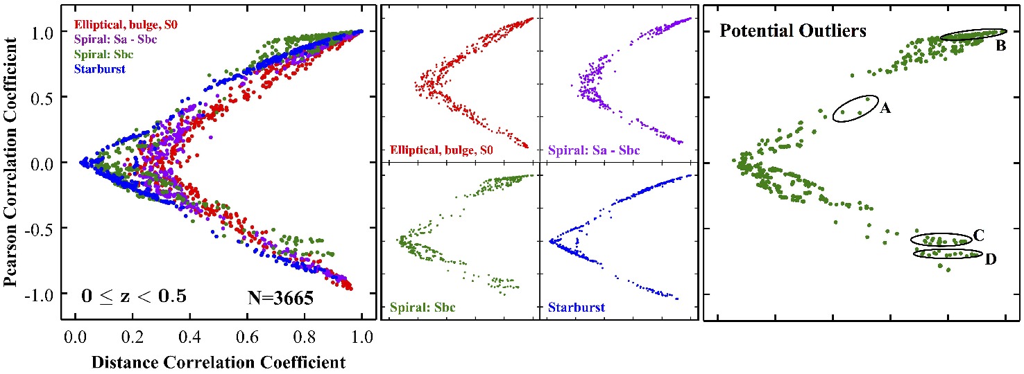
Figure 1: Pearson correlation coefficient vs. distance correlation coefficient for 528 pairs of variables, calculated for galaxies with redshift $0\leq z<0.5$. The subplots for each galaxy type are shown in four middle frames together with the superposition of the four subplots in the large left frame. The locations of potential outlier pairs in the scatter plot for Type 3 (Spiral: Sbc) galaxies is also shown in the large right frame.

I will also discuss data arising in the national discussion of the relationship between homicide rates and the strength of state gun laws. A Washington Post columnist has claimed that there is “Zero correlation between state homicide rate and state gun laws” [8]. Indeed, calculation of the corresponding empirical Pearson coefficient detects no statistically significant relationship between those variables. However, a distance correlation analysis of the data discovers overwhelming evidence that, when the states are partitioned by region or by median population density, there is a strong relationship between the two variables.

There is also the intriguing formula (4) for the empirical distance covariance. Behind that formula lies a remarkable singular integral: For $x\in\mathbb{R}^{p}$ and $\hbox{Re}(\alpha)\in(0,2)$,

$$\int_{\mathbb{R}^{p}}\frac{1-e^{{\mathrm{i}}\langle s,x\rangle}}{\|s\|^{p+\alpha}}\hbox{d}s=\frac{2\pi^{p/2}\Gamma\big{(}1-\tfrac{1}{2}\alpha\big{)}}{\alpha 2^{\alpha}\Gamma\big{(}\tfrac{1}{2}(p+\alpha)\big{)}}\|x\|^{\alpha},$$

with absolute convergence for all $x$. We shall describe generalizations of this singular integral arising from truncated Maclaurin expansions of the cosine function and in the theory of spherical functions on symmetric cones.

References

• [1] Dueck, J., Edelmann, D., and Richards, D. (2017). Distance correlation coefficients for Lancaster distributions. Journal of Multivariate Analysis, 154, 19–39.
• [2] Feuerverger, A. (1993). A consistent test for bivariate dependence. International Statistical Review, 61, 419–433.
• [3] Freeman, K. (1947). Ancilla to The pre-Socratic philosophers: a complete translation of the fragment in Diels Fragmente der Vorsokratiker. Sixth Impression. Blackwell. 1971.
• [4] MartΓ­nez-GΓ³mez,Β E., Richards,Β M.Β T., and Richards,Β D.Β St.Β P.Β (2014). Distance correlation methods for discovering associations in large astrophysical databases. Astrophysical Journal, 781, 39 (11 pp.).
• [5] Richards, M. T., Richards, D. St. P., and MartΓ­nez-GΓ³mez, E. (2014). Interpreting the distance correlation results for the COMBO-17 survey. Astrophysical Journal Letters, 784, L34 (5 pp.).
• [6] SzΓ©kely, G. J., Rizzo, M. L., and Bakirov, N. K. (2007). Measuring and testing independence by correlation of distances. Annals of Statistics, 35, 2769–2794.
• [7] SzΓ©kely, G. J., and Rizzo, M. (2009). Brownian distance covariance. Annals of Applied Statistics, 3, 1236–1265.
• [8] Volokh, E. (2015). Zero correlation between state homicide rate and state gun laws. The Washington Post, October 6, 2015.
• [9] Wolf, C., Meisenheimer, K., Rix, H.-W., Borch, A., Dye, S., and Kleinheinrich, M. (2003). The COMBO-17 survey: Evolution of the galaxy luminosity function from 25000 galaxies with $0.2<z<1.2$. Astronomy & Astrophysics, 401, 73–98.