On the nature of off-limb flare continuum sources detected by SDO/HMI

Abstract

The Helioseismic and Magnetic Imager onboard the Solar Dynamics Observatory has provided unique observations of off-limb flare emission. White-light (WL) continuum enhancements were detected in the ”continuum” channel of the Fe 6173 Å  line during the impulsive phase of the observed flares. In this paper we aim to determine which radiation mechanism is responsible for such an enhancement being seen above the limb, at chromospheric heights around or below 1000 km. Using a simple analytical approach, we compare two candidate mechanisms, the hydrogen recombination continuum (Paschen) and the Thomson continuum due to scattering of disk radiation on flare electrons. Both mechanisms depend on the electron density, which is typically enhanced during the impulsive phase of a flare as the result of collisional ionization (both thermal and also non-thermal due to electron beams). We conclude that for electron densities higher than $10^{12}$ cm^-3, the Paschen recombination continuum significantly dominates the Thomson scattering continuum and there is some contribution from the hydrogen free-free emission. This is further supported by detailed radiation-hydrodynamical (RHD) simulations of the flare chromosphere heated by the electron beams. We use the RHD code FLARIX to compute the temporal evolution of the flare heating in a semi-circular loop. The synthesized continuum structure above the limb resembles the off-limb flare structures detected by HMI, namely their height above the limb, as well as the radiation intensity. These results are consistent with recent findings related to hydrogen Balmer continuum enhancements, which were clearly detected in disk flares by the IRIS near-ultraviolet spectrometer.

1 Introduction

Off-limb observations of solar flares are rather rare but they can provide an important constraint on the height variation of different flare emissions. Occasionally, off-limb flares have been detected in the H$\alpha$ line and some other lines, but the so-called white-light flares (WLF) observed on the disk in the visible light have never been seen above the limb from the ground. Only recently has the full-disk monitoring of the Sun by SDO allowed such detections through the Helioseismic and Magnetic Imager (HMI) instrument, thanks to observing conditions in space. What we see above the limb at the outermost wavelength channels of the Fe I 6173 Å  line is believed to be continuum emission unaffected by the line itself. This channel is often used to detect the white-light (WL) continuum in disk flares and various such observations have been reported in the literature. However, above the limb, only a few cases have been analyzed (Martínez Oliveros et al. (2012), Krucker et al. (2015)) that challenge our understanding of the continuum formation in flares.

WL continuum enhancements seen on the disk inside the flare ribbons (e.g. Kuhar et al. (2016)) are normally interpreted as being due to either hydrogen recombination emission in the Paschen continuum (below the series limit at 8203 Å), or photospheric (i.e. H^-) continuum enhancement, or a combination of both. However, the continuum enhancement on the disk relative to the photospheric brightness itself (i.e. the contrast) is usually low in the visible range (typically below 10%) and this makes it very difficult to disentangle the two emission mechanisms (see, e.g. Kerr & Fletcher (2014)). Note that the Paschen recombination continuum intensity is related to the Balmer continuum intensity and the latter was recently detected by IRIS in its near-ultraviolet (NUV) channel (Heinzel & Kleint (2014), Kleint et al. (2016)). There is no suitable flare observation yet above the limb by IRIS that would show the Balmer continuum. However, contrary to disk observations (both ground-based and using HMI), the off-limb HMI WL continuum detection can reveal important height distributions of the emissivity and thus can help to disentangle the various possible mechanisms.

Another HMI off-limb observation of a WL emission comes from high-lying (33 Mm) flare loops seen during the gradual phase of a flare (Saint-Hilaire et al., 2014), where significant degree of linear polarization was also detected. This emission was then interpreted as being due to the Thomson scattering on free electrons inside the loops.

In this paper we investigate the nature of the off-limb emission at flare footpoints, using simple analytical relations for WL emissivities and using also using the results of radiation-hydrodynamical (RHD) simulations of flare heating by electron beams. For the latter we use the RHD code FLARIX. We compare the synthetic continuum intensity with that detected by HMI and discuss constraints set by HMI off-limb observations on flare-heating models.

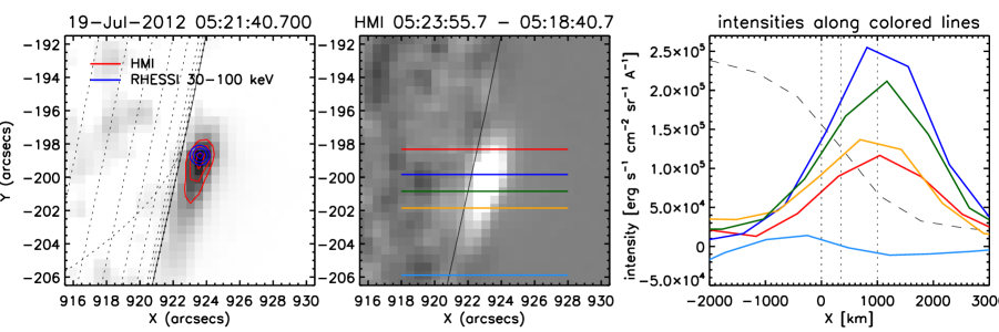
Figure 1: Co-spatial white-light and hard X-ray flare footpoints seen above the solar limb for the 20120719 flare. Note that all curves go to zero in the corona above the flare, due to the subtraction of the pre-flare emission. The intensity thus represents pure flare continuum emission. The three vertical dashed lines on the rightmost panel represent the zero height at $\tau_{5000}=1$, the photospheric limb at height 350 km, and chromospheric height at 1000 km, respectively.

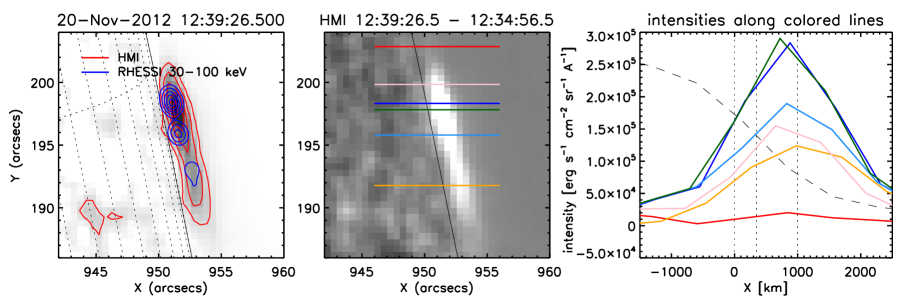
Figure 2: Same as a) but for the 20121120 limb flare

2 SDO/HMI Off-limb Flare Observations

To obtain the observed intensities of off-limb sources, we analyze hmi.Ic_45s SDO/HMI data. We investigate two limb flares: the M7.7 flare on 2012 July 19 and the M1.7 flare on 2012 November 20. Krucker et al. (2015) determined the heights of their WL emission above $\tau_{5000}=1$ to be 824 $\pm$ 70 km and 799 $\pm$ 70 km, respectively. The left panel of Fig. 1 is adapted from Krucker et al. (2015) and shows a negative difference image for the WL emission. The red contours trace the HMI emission and blue contours show hard X-ray emission at 30-100 keV, which is co-spatial to the continuum emission. The middle panel shows a difference image at the time of maximum enhancement. The limb is drawn by the SSW routine plot_map.pro and is based on a calculation. Intensity cuts along the five horizontal lines are shown in the right panel. We converted from DN/s to absolute units by taking the HMI disk-center intensity and setting it to the continuum value at 6173 Å  of 0.315 $\times$ 10⁷ erg s^-1 cm^-2 sr^-1 Å^-1 from Brault & Neckel’s atlas (Neckel, 1994). Here we determined the limb as the inflexion point of the pre-flare limb darkening intensity, which differs from the calculated limb of plot_map by about one pixel ($0.\!\arcsec 5$) and we assigned it the height 350 km (the $x$-axis in the right panel). The maximum observed enhancements are $3\ \times\ 10^{5}\ \mbox{erg s}^{-1}\ \mbox{cm}^{-2}\ \mbox{sr}^{-1}\ \AA^{-1}$, and the spatial and temporal variations are significant. Our height estimate of the peak emission from Figures 1 and 2 is in the range of 800 - 1100 km above the level of $\tau_{5000}=1$.

3 Mechanisms of the WL Continuum Emission

As stated in the introduction, the WL enhancement on the disk consists of the expected photospheric contribution due to H^- and the hydrogen recombination continuum, which is the Paschen continuum around the 6173 Å  HMI line. Above the limb at chromospheric heights, we expect that HMI observations should reveal only the Paschen component. However, some HMI off-limb observations have been interpreted in terms of Thomson scattering and we therefore devote this section to an analytical estimation of the relative importance of the Paschen vs. Thomson components. Moreover, we estimate the importance of the hydrogen free-free emission above the limb.

3.1 Paschen Continuum Emission Due to Hydrogen Recombination

Hydrogen in the flaring chromosphere is highly ionized due to a strong temperature increase (thermal collisional ionization), but also due to collisions of hydrogen with non-thermal electrons from the beam. Protons then capture free thermal electrons (note that the non-thermal ionization of hydrogen produces electrons that are finally thermalized) and create neutral hydrogen atoms, a process called hydrogen recombination. It has been demonstrated that the possible capture of non-thermal electrons from the beam is quite negligible.

The Paschen continuum emissivity is then expressed as (Hubeny & Mihalas, 2014)

$$\eta_{\nu}^{i}=n_{\rm e}n_{\rm p}F_{i}(\nu,T)\,,$$ (1)

where $i$=3 (Paschen continuum), $n_{\rm e}$ and $n_{\rm p}$ are the electron and proton densities, respectively, $\nu$ is the frequency of the observed emission, and $T$ is the kinetic temperature of the source. The function $F_{i}$ has the form

$$F_{i}(\nu,T) = 1.166\times 10^{14}g_{\rm{II}}(i,\nu)T^{-3/2}B_{\nu}(T)\times$$ (2)

$${\rm e}^{h\nu_{i}/kT}(1-{\rm e}^{-h\nu/kT})/(i\nu)^{3}\,.$$

Here, $\nu_{i}$ is the frequency at the continuum head, $g_{\rm II}$ is the Gaunt factor, $B_{\nu}(T)$ is the Planck function, and $h$ and $k$ are the Planck and Boltzmann constants, respectively. For optically thin plasma, we multiply this emissivity by the line-of-sight geometrical extension of the source to obtain the specific intensity of the continuum radiation $I(\nu)$.

3.2 Thomson Scattering

Here we compute the continuum intensity around the 6173 Å  line due to Thomson scattering on flare-loop electrons. The scattering is assumed to be coherent and isotropic. The emissivity is given by the standard formula (e.g. Hubeny & Mihalas (2014))

$$\eta_{\nu}=n_{\rm e}\sigma_{\rm{T}}J(\nu)\,,$$ (3)

where $\sigma_{\rm{T}}$ = 6.65 $\times$ 10^-25 cm² is the absorption cross section for Thomson scattering and $J(\nu)$ is the diluted photospheric WL radiation. The latter is obtained from the disk-center continuum intensity, multiplied by the dilution factor for chromospheric heights. A purely geometrical dilution factor would be around 0.5 for low heights, up to 1000 km. However, here we take into account the center-to-limb variations of the photospheric continuum intensity and thus the effective dilution factor is 0.354 at 6174 Å  (Jejčič & Heinzel (2009)). The disk-center continuum intensity at 6173 Å  is $3.96\ \times\ 10^{-5}\ \mbox{erg s}^{-1}\ \mbox{cm}^{-2}\ \mbox{sr}^{-1}\ \mbox{Hz}^{-1}$, as linearly interpolated from Allen’s tables (Cox, 2000). This, multiplied by $0.354$ gives a value of $J(\nu)=1.40\ \times\ 10^{-5}\ \mbox{erg s}^{-1}\ \mbox{cm}^{-2}\ \mbox{sr}^{-1}\ \mbox{Hz}^{-1}$, which is used in our modeling. In reality, the scattering is strictly coherent only in the electrons’ rest-frames, but due to their thermal motions the scattered photons are Doppler-shifted. In the case of scattering of the photospheric line radiation, this leads to a smearing of the scattered line profile, which is well known in the coronal WL spectra. In our case, the non-coherent scattering of the 6173 Å  line radiation could somewhat affect our results, but using the above formula we get an upper limit for the continuum intensity due to Thomson scattering. The assumption of isotropic scattering is standard in atmospheric modeling (Hubeny & Mihalas, 2014).

3.3 Relative Importance of the Paschen and Thomson Continuum above the Limb

From the above equations we see that the ratio of the intensities of the Paschen and Thomson continuum will be proportional to the electron density under the assumption that $n_{\rm e}=n_{\rm p}$, which is well satisfied in the chromosphere where the helium contribution to the electron density is small:

$$\frac{I^{\rm Pa}}{I^{\rm Th}}=n_{\rm e}\frac{F_{i}}{\sigma_{\rm T}J(\nu)}\,.$$ (4)

We show this ratio for a range of electron densities and for various plasma temperatures (Figure 3). While at lower electron densities, say, below 10¹² cm^-3, the Thomson continuum starts to dominate over the Paschen continuum, for the higher densities usually met in the flaring chromosphere, the Paschen continuum dominates. The ratio decreases with increasing kinetic temperature, which is due to the nature of the recombination process. Since the electron densities in stronger flares can reach 10${}^{13}-10^{14}\ \mbox{cm}^{-3}$ (e.g. Avrett et al., 1986), we immediately see that any off-limb emission must be quite dominated by the Paschen continuum. In the next section we will confirm this estimate using and RHD simulation of the electron-beam heated atmosphere.

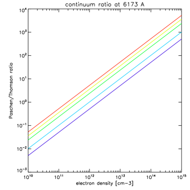
Figure 3: Theoretical ratio of the Paschen to Thomson continuum intensity at 6173 Å, as a function of the electron density. The colors correspond to different temperatures: red - 6000 K, yellow - 10,000 K, green - 15,000 K, blue - 30,000 K, magenta - 50,000 K.

3.4 Hydrogen Free-Free Continuum Emission

So far we have discussed the most explored mechanisms of the WL emission in solar flares. However, in the optical range and for longer wavelengths, hydrogen free-free continuum emission may also contribute, namely at higher temperatures. One can easily express the ratio between free-free and Paschen free–bound continuum intensity as

$$\frac{I^{\rm ff}}{I^{\rm Pa}}=8.55\times 10^{-5}T{\rm e}^{h\nu_{i}/kT}\,,$$ (5)

using the expressions for emissivities from Hubeny & Mihalas (2014) and assuming that the Gaunt factors are around unity. This immediately shows that such a ratio substantially increases with increasing temperature, being equal to 0.15 for $T=10,000$ K, 0.71 for 20,000 K, and 1.43 for 30,000 K. Therefore, between $T=20,000$ K and 30,000 K, the free-free continuum emission starts to dominate over the Paschen continuum.

4 RHD Simulation with the FLARIX Code

In this section we present our RHD simulation of the evolving flare chromosphere and use it to visualize the continuum source above the limb. The RHD code FLARIX (see, e.g. Varady et al., 2010; Heinzel et al., 2016) was run for a specific model of the electron-beam heating inside a semi-circular loop extending from the photosphere to coronal heights. The initial model was the VAL-C type atmosphere (Vernazza et al., 1981) with an enhanced pressure/density. The radiation losses of this starting atmosphere were balanced by a constant heating term to assure initial hydrostatic equilibrium. The electron beam has a triangular temporal variation of the energy flux lasting 10 s, with a peak flux of 0.75 $\times$ 10¹¹ erg s^-1 cm^-2 at time $t$=5 s. The spectral index of the beam was $\delta=4$. Optically thick radiation losses and hydrogen non-thermal collisional rates have been computed at chromospheric heights. To synthesize the off-limb continuum structure, we use a snapshot at time $t$=4 s from the whole FLARIX simulation. At this time, just before the peak of the energy deposit, the middle chromosphere is already highly ionized and thus a further increase of the flux practically does not affect our results. The peak flux derived from an analysis of RHESSI spectra of these flares is higher, but that seems to affect the atmospheric electron density only marginally. Moreover, electron-beam fluxes exceeding 10¹¹ erg s^-1 cm^-2 could produce a significant return current in the chromosphere and this is not yet properly treated in the available RHD codes. In Figures 4 and 5 we show the height variations of the kinetic temperature and electron density at this time, respectively.

Figure 4: Snapshot of the height variation of the kinetic temperature from the FLARIX simulation at time $t$=4 s. For comparison, we also show the temperature structure of a pre-flare VAL3C atmosphere with an enhanced plasma density (dashed line). The zero height (the limb) is located at 350 km above the level of $\tau_{5000}=1$, i.e. the height scale is shifted compared to Figures 1 and 2.

Figure 5: Snapshot of the height variations of the electron density from the FLARIX simulation at time $t$=4 s. For comparison, we also show the electron density of a pre-flare VAL3C atmosphere with an enhanced plasma density (dashed line). The zero height (the limb) is located at 350 km above the level of $\tau_{5000}=1$.

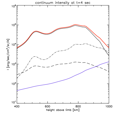
Figure 6: Vertical variations of the line-of-sight total continuum intensity for thickness 1000 km, from our FLARIX simulation at time $t$=4 s (red line). This is mostly dominated by the Paschen continuum (full black line), while the dotted-dashed line shows the hydrogen free-free contribution and the dashed line shows the Thomson scattering component. The blue line indicates the energy deposit rate due to the electron-beam precipitation. The zero height (the limb) is located at 350 km above the level of $\tau_{5000}=1$.

From Figure 5 we immediately see that the electron density in the middle chromosphere reaches values above 10¹³ cm^-3 which means that, according to our plot in Figure 3, the continuum emission above the limb is fully dominated by the Paschen continuum, while the Thomson scattering is quite negligible. Note that the Paschen-continuum is optically thin under these conditions, so the line-of-sight integration of the emissivity is straightforward and gives the synthetic intensity.

4.1 1.5D Visualization of the Off-limb Structure

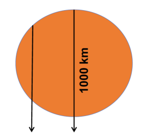
Figure 7: Horizontal cross section of the flare loop showing the two selected lines of sight along which we integrate the continuum emissivities. The loop diameter is 1000 km.

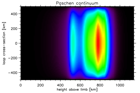
Figure 8: 1.5D visualization of the off-limb structure from FLARIX simulation at time $t$=4 s. The zero height (the limb) is located at 350 km above the level of $\tau_{5000}=1$.

Assuming that the flare loop thickness is 1000 km, we integrate the continuum emissivity along the off-limb line of sight at each atmospheric height above the limb from 0 to 1200 km. For a given height we assume a constant temperature and electron density along the line of sight, both given by the FLARIX simulation. The resulting height-dependent continuum intensity along the loop axis is shown in Figure 6. From this plot we already see that the off-limb structure extends from about 450 to 950 km above the limb, which is consistent with HMI observations. Note that the HMI brightness is displayed in Figures 1 and 2 on a scale where zero is at the level of $\tau_{5000}=1$ and thus it goes to larger heights compared to Figures 4-6, where zero (the limb) is at photospheric height 350 km. Also, the intensity, which reaches $10^{5}\ \mbox{erg s}^{-1}\ \mbox{cm}^{-2}\ \mbox{sr}^{-1}\ \AA^{-1}$ is consistent with that from HMI as shown in Figure 1, provided that the actual geometrical thickness of the off-limb structure is a factor up to 3 larger than our nominal value 1000 km. This is quite plausible because a direct inspection of the loop-system geometry from STEREO observations reveals larger line-of-sight volumes (see, e.g.  Krucker et al., 2015). Rather complex projection effects of the whole loop arcade could also be responsible also for the wider height distribution of the continuum emission (see the rightmost panels in Figures 1 and 2), compared to our single-loop simulation. In Figure 6 we also separately show the hydrogen free-free continuum intensity that starts to dominate the Paschen continuum at temperatures above 20,000 K and the Thomson continuum intensity that is about two orders of magnitude weaker compared to the Paschen continuum. For reference, we also add the curve of the energy deposit due to the electron-beam energy losses (in arbitrary units). In the low chromosphere, the energy deposit is small compared to that at higher layers, thus the atmosphere does not differ much from the initial state. Note that the limb in these plots is actually placed at a height of 350 km above the zero atmospheric height used in FLARIX, i.e. the photospheric height where $\tau_{5000}=1$ in the quiescent atmosphere. The value of 350 km comes from Table I of Lites (1983) and indicates the limb height at wavelength 6000 Å. This should correspond to the limb as detected by HMI.

As a next step we have performed a line-of-sight integration of the Paschen continuum emissivity along the rays crossing a circular loop with a nominal diameter of 1000 km (see the top view of such loop in Figure 7), assuming again that the temperature and electron density in the horizontal plane are constant and equal to values computed by FLARIX at a given atmospheric height. Since FLARIX represents a 1D modeling along the loop axis (in the vertical direction), while the formal transfer solution is made along rays crossing our circular loop horizontally, we call this kind of spectrum synthesis a 1.5D radiative-transfer visualization. The result is displayed in Figure 8, where the horizontal axis shows the height above the limb and the vertical axis gives the distance from the loop axis toward its surfaces at $\pm$ 500 km (the total thickness of the loop is 1000 km). Figure 8 shows the off-limb distribution of the Paschen-continuum brightness (the intensity values along the loop axis, i.e. for $y$=0, can be inferred from Figure 6). From Figure 8 we see that below 400 km the continuum emission is quite negligible and the same also applies for heights above 1000 km (where the free-free emission already dominates). The brightness variations along the $x$-axis are mainly due to the height variations of the electron density computed by FLARIX. Note that the intensity is roughly proportional to $n_{\rm e}^{2}$. The main peak is between 750 and 800 km above the limb, similar to HMI observations of selected structures (see Figure 1). The less bright secondary peak around the height 500 km, not seen in the HMI observations (note, however, that we did not perform any convolution with the HMI PSF), is the result of our particular simulation and different FLARIX models will likely lead to different height distributions of the continuum emission.

5 Discussion and Conclusions

Our results set quantitative constraints on the mechanisms of WL emission in solar flares, the issue frequently referred to as the “WLF mystery”. Contrary to more frequent disk observations where the WL enhancement is likely due to a mixture of Paschen-continuum emission and enhanced photospheric H^- continuum, the off-limb observations naturally eliminate the latter contribution. Our estimates, together with detailed numerical simulations, lead to the conclusion that the observed WL enhancement detected by SDO/HMI is dominated by the hydrogen Paschen continuum (Brackett continuum is about 5 time weaker), with a small contribution from the free-free mechanism. Thomson scattering on chromospheric electrons is also enhanced during the flare, compared to a pre-flare atmosphere, but because the ratio of Paschen/Thomson emissivity scales linearly with the electron density, the Paschen continuum significantly dominates, namely in stronger flares. However, in the case of the so-called ’post-flare’ loops observed by HMI in WL at high altitudes around 33 Mm, Saint-Hilaire et al. (2014) detected significant $Q$-polarization, as expected from pure Thomson scattering at such altitudes and wavelengths, for electron densities below 10¹¹ cm^-3. This is consistent with our estimates presented in Figure 3. Note that in solar prominences where the electron densities are even lower, the WL continuum is indeed dominated by the Thomson scattering (Jejčič & Heinzel, 2009). At lower altitudes around 15 Mm, Saint-Hilaire et al. (2014) found a dominant non-Thomson component (at densities around 10¹² cm^-3) and suggested their free-free and free-bound origin.

Our simulations, and namely 1.5D visualizations, are based on a circular loop-like model for which we took a diameter of 1000 km. Several such loops can be aligned along the line of sight, as STEREO observations of this flare do indicate. However, in reality these flare loops can reach diameters as small as 100 km, as recent high-resolution observations suggest (Jing et al. (2016)). The latter authors conclude that the whole flare loop system (they show cool ’post’ flare loops, but those result from previous hot loops considered here) has a very small filling factor compared to volumes visible at much lower spatial resolutions like those seen by HMI or RHESSI. This issue will set new constraints on future quantitative modeling, where also the assumed electron-beam fluxes may reach even higher values.

We have also investigated the surrounding chromospheric opacity of the bound-free Paschen continuum. Using the quiet-Sun model VAL-C we have integrated the opacity along the off-limb lines of sight at various chromospheric heights where the flare emission is detected. The corresponding optical thicknesses of the Paschen continuum at the HMI wavelength were found to be quite small, around 10^-3 just above the limb and decreasing upward to about 1.4 $\times 10^{-4}$ at heights around 800 km above the limb where our simulations give the maximum of the flare continuum emission. Therefore, we do not expect the surrounding chromosphere to have any effect on the flare continuum visibility. In this estimate, we neglected the possible influence of spicules seen above the limb; in actuality, any non-negligible continuum opacity would lead to an obscuration of the off-limb flare and also would produce a bright ring in the chromosphere surrounding the solar limb, which,for example, is observed in H$\alpha$, but not in WL.

Off-limb observations of flares with HMI could also provide us with information about the formation height of the iron line 6173 Å. It is well known that the cores of many metallic (iron) lines are enhanced during flares (see, e.g., the recent paper by Kleint et al., 2017) and it would be very interesting to see at which heights they are formed during the flare - these are normally photospheric lines when formed in an undisturbed atmosphere. However, it is assumed that the outermost wavelength channels of HMI do not contain line emission and are thus solely representative of the WL continuum emission. Our inspection of HMI off-limb spectra indicates that the intensity enhancement is about the same at all wavelengths. But the Thomson scattering of the 6173 Å  line radiation can result in a lowering of the WL intensity, compared to our model in which the pure continuum scattering is considered for simplicity.

Finally, it would be quite interesting to obtain limb observations of flares by IRIS, in order to detect an off-limb Balmer-continuum emission, similar to that found on the disk by Heinzel & Kleint (2014) and Kleint et al. (2016). This, together with the HMI observations discussed in this paper, could provide a unique constraint on the radiation mechanisms of white-light flares. Off-limb emission in the hydrogen Balmer continuum would observationally constrain the chromospheric losses in this continuum. Such losses have been shown to be dominant in the region of the electron-beam energy deposit and thus they play a crucial role in the energy balance (Heinzel et al., 2016). Based on the results of the existing HMI off-limb and IRIS on-disk observations of the continuum emission, the issue of WLFs becomes less “mysterious”, although the true mechanism behind the photospheric (on-disk) WL enhancement is still not well understood.

References

- Avrett et al. (1986) Avrett, E. H., Machado, M. E., & Kurucz, R. L. 1986, in The Lower Atmosphere of Solar Flares, ed. D. F. Neidig, Proc. NSO Wokshop, Sunspot, 216, 216–281
- Cox (2000) Cox, A. N. 2000, Allen’s astrophysical quantities (Springer)
- Heinzel et al. (2016) Heinzel, P., Kašparová, J., Varady, M., Karlický, M., & Moravec, Z. 2016, in IAU Symposium, Vol. 320, Solar and Stellar Flares and their Effects on Planets, ed. A. G. Kosovichev, S. L. Hawley, & P. Heinzel (Cambridge Univ. Press), 233–238
- Heinzel & Kleint (2014) Heinzel, P., & Kleint, L. 2014, ApJ, 794, L23
- Hubeny & Mihalas (2014) Hubeny, I., & Mihalas, D. 2014, Theory of Stellar Atmospheres (Princeton University Press)
- Jejčič & Heinzel (2009) Jejčič, S., & Heinzel, P. 2009, Sol. Phys., 254, 89
- Jing et al. (2016) Jing, J., Xu, Y., Cao, W., et al. 2016, Scientific Reports, 6, 24319
- Kerr & Fletcher (2014) Kerr, G. S., & Fletcher, L. 2014, ApJ, 783, 98
- Kleint et al. (2016) Kleint, L., Heinzel, P., Judge, P., & Krucker, S. 2016, ApJ, 816, 88
- Kleint et al. (2017) Kleint, L., Heinzel, P., & Krucker, S. 2017, ApJ, 837, 160
- Krucker et al. (2015) Krucker, S., Saint-Hilaire, P., Hudson, H. S., et al. 2015, ApJ, 802, 19
- Kuhar et al. (2016) Kuhar, M., Krucker, S., Martínez Oliveros, J. C., et al. 2016, ApJ, 816, 6
- Lites (1983) Lites, B. W. 1983, Sol. Phys., 85, 193
- Martínez Oliveros et al. (2012) Martínez Oliveros, J.-C., Hudson, H. S., Hurford, G. J., et al. 2012, ApJ, 753, L26
- Neckel (1994) Neckel, H. 1994, in Poster Proceedings from IAU Colloquium 143: The Sun as a Variable Star: Solar and Stellar Irradiance Variations, ed. J. M. Pap, C. Frohlich, H. S. Hudson, & S. K. Solanki (Cambridge Univ. Press), 37
- Saint-Hilaire et al. (2014) Saint-Hilaire, P., Schou, J., Martínez Oliveros, J.-C., et al. 2014, ApJ, 786, L19
- Varady et al. (2010) Varady, M., Kasparova, J., Moravec, Z., Heinzel, P., & Karlicky, M. 2010, IEEE Transactions on Plasma Science, 38, 2249
- Vernazza et al. (1981) Vernazza, J. E., Avrett, E. H., & Loeser, R. 1981, ApJS, 45, 635