Exact wave functions and entropies of the one dimensional Regularized Calogero model

Abstract

The divergence in the interaction term of the Calogero model can be prevented introducing a cutoff length parameter, this modification leads to a quasi-exactly solvable model whose eigenfunctions can be written in terms of Heun’s polynomials. It is shown both, analytical and numerically. that the reduced density matrix obtained tracing out one particle from the two-particle density operator can be obtained exactly as well as its entanglement spectrum. The number of non-zero eigenvalues in these cases is finite. Besides, it is shown that taking the limit in which the cutoff distance goes to zero, the reduced density matrix and finite entanglement spectrum of the Calogero model is retrieved. The entanglement Rényi entropy is also studied to characterize the physical traits of the model. It is found that the quasi-exactly solvable character of the model is put into evidence by the entanglement entropies when they are calculated numerically over the parameter space of the model.

I Introduction

The Calogero model Calogero1969 occupies a remarkable place in theoretical and mathematical physics. It has been linked, or is an integral part of advances made in quantum Hall effect Azuma1994 , random matrices Altshuler1993 , integrability Poly1993 , Yang-Mills theory Gorsky1994 , etc.

Remarkably, the Calogero model variants, the deformed Chalykh1998 ; Atai2017 , the different generalizations Polychronakos1999 ; Znojil2001 and the rectified ones Downing2017 , inherit many of its properties, a trend that was acknowledged from very early by Sutherland Sutherland1971 . More recently, it has been shown that the $p-$reduced density matrix (p-RDM) of a $N$-particle one-dimensional Calogero model can also be obtained exactly opos15 , as well as the entanglement spectrum, for a discrete set of the strength interaction parameter (let us remember that the p-RDM matrix is obtained when $(N-p)$ particles are traced out of the density matrix of an $N-$particle system). Besides, at these values the Rényi entanglement entropies show non-analytical behaviour Garagiola2016 in contradistinction with the von Neumann entropy.That the Calogero model admits exact reduced density matrices was also noted by Katsura and Hatsuda Katsura2007 .

The harmonic confinement potential, present in all the variants of the model, was included more as a mean to keep the particles bounded, since the interaction between them is mainly repulsive, rather than as a model for an implementable potential. Nevertheless, the advances made in cold confined gases and quantum dots make the model applicable to analyze actual experimental setups.

Quasi-exactly solvable models quasi1 , as the so called spherium Ezra1982 ; Ezra1983 ; Loos2009 , or other electron systems confined in boxes with different geometries, as square Alavi2000 ; Ghosh2005 , cylindrical Ryabinkin2010 and spherical Jung2004 are of interest because they are more amenable of analytical treatment than boundless ones. Besides its behaviour is quite different from the observed in extended systems, so they posed new challenges that allow to improve the DFT method Loos2014a ; Loos2014b . They are benchmarks where many numerical methods can be tested Loos2010 ; Jung2004 ; Jung2003 and model strongly confined electron systems. The condition of quasi-exactly solvable means that the spectrum and the eigenfunction are exactly known in a discrete set of the Hamiltonian parameters. Recently there has been a flurry of activity in this subject Loos2009 ; Downing2016 ; Tognetti2016 ; Downing2013 ; Downing2017 , while early examples, dealing with the same quasi-exactly solvable model, can be found in the works of Kais et. al. Kais1989 and Taut Taut1993 . The recent advances made in one- and two-particle quasi-exactly solvable models rely heavily on the properties of the polynomial solutions of the Heun differential equation Heun1 .

The broad application to many different problems in classical and quantum physics of the Heun’equations and its polynomial solutions has been made possible by the work of Fiziev Fiziev2010 , in particular to the dynamics of a rotor vibratory giroscope Motsepe2014 , the calculation of natural occupation numbers in two electron quantum-rings Tognetti2016 , the solution of the Schrödinger equation for a particle trapped in a hyperbolic double-well potential Downing2013 , the problem of two electrons confined on a hypersphere Loos2009 , one electron in crossed inhomogeneous magnetic and homogeneous electric fields Downing2016 , and in the study of normal modes in non-rotating black holes Fiziev2011 . The recent and salient role played by the Heun functions, and its foreseeable future, in natural sciences is depicted in the Introduction of Ref. Fiziev2012 .

Quite recently, Downing has reported the analytical solutions of a two-electron quantum model Downing2017 . In the model analyzed, the two particles interact via a regularized potential that decays as the inverse of the distance between the particles squared, i.e. the model is a regularized Calogero model. The regularization prevents the divergence of the potential when the distance between the particles goes to zero, introducing a short distance cutoff parameter $d$. Remarkably, the model is quasi-exactly solvable so, for a given value of $d$, the exact two-particle wave function can be obtained only for a discrete set of values of the interaction strength parameter $g$, as is usually denoted in the context of the Calogero model. At these values, the two-particle wave function is a polynomial function of the inter-particle distance. As has been shown in Ref. opos15 , when the wave function of a multi-particle Calogero model can be written as the product of a polynomial function depending on the inter-particles distances, times other functions that depend separately on the coordinates of each particle, then the $p$-RDM and the entanglement spectrum can be both obtained exactly. Since the Rényi entropy also shows a very particular behavior for these discrete set of values, it does beg the question of how many of these features are inherited by the regularized model. To this end, we study the exact solutions of the one-dimensional two particle regularized model, both their symmetric and anti-symmetric solutions under particle interchange and their reduced density matrices. Even though this is a quasi-exactly solvable model we calculate numerical solutions to study the whole Hamiltonian parameter space. A motivation to perform such exact calculations of entropies arises from the need of stringent benchmarks that assess the accuracy of numerical approximations when they are applied to confined electron systems Jiao2017 .

This paper is organized as follows: The regularized Calogero model is presented in Section II. In Section III the exact symmetric wave functions are thoroughly analyzed while the antisymmetric ones are the subject of Section IV. The Rényi and von Neumann entropies for the exact two-particle states, together with numerical approximations, are presented in Section V. Finally, a discussion of the results and some open questions are presented in Section VI.

II The model and its eigenfunctions

Recently, Downing Downing2017 showed that the three-dimensional two-particle regularized Calogero model is solvable for a discrete set of values of the interacting parameter. In this work, we address the one dimensional two-particle regularized Calogero Hamiltonian

$$H=h(1)\,+\,h(2)+\frac{g}{x_{12}^{2}+2\,d^{2}}\,,$$ (1)

where

$$h(i)=\frac{1}{2}\,p_{i}^{2}+\frac{1}{2}\,x_{i}^{2}\;\;\mbox{and}\;\;\,x_{12}\,=\,|x_{1}-x_{2}|\,.$$ (2)

In particular, we look for a discrete set of exact two-particle symmetric or antisymmetric wave functions. We do not assume particular values for the spin variable, so the symmetric and antisymmetric functions can be used to construct two-fermions or two-bosons solutions depending on the symmetry of the spinorial part of the quantum state.

With the coordinate transformation

$$X\,=\,\frac{1}{\sqrt{2}}(x_{1}+x_{2})\;\;\;;\;\;\;x\,=\,\frac{1}{\sqrt{2}}(x_{1}-x_{2})\,,$$ (3)

the Hamiltonian Eq. (1) takes the form $H=H_{X}+H_{x}$, where

$$H_{X}\,=\,-\frac{1}{2}\frac{d^{2}}{dX^{2}}+\frac{1}{2}X^{2}\;\;\;;$$ (4a)

$$H_{x}\,=\,-\frac{1}{2}\frac{d^{2}}{dx^{2}}+\frac{1}{2}x^{2}+\frac{g/2}{x^{2}+d^{2}}\,.$$ (4b)

The eigenfunctions will be the product of eigenfunctions of each Hamiltonian $\psi(x_{1},x_{2})=\Psi(X)\,\psi(x)$, and the eigen-energies the sum of the eigenvalues, $E=E_{X}+E_{x}$. For the center of mass Hamiltonian Eq.(4a) we will consider the ground state

$$E_{X}=\frac{1}{2}\;\;\;;\;\;\;\Psi(X)\,=\,\frac{1}{\pi^{1/4}}e^{X^{2}/2}\,.$$ (5)

This eigenfunction is symmetric, and the Hamiltonian Eq. (4b) is even in $x$, that means that the even (odd) eigenfunctions of the Hamiltonian Eq. (4b) correspond to totally symmetric (antisymmetric) eigenfunctions under particle interchange. The odd eigenfunctions of Hamiltonian Eq. (4b) are the three-dimensional solutions written by Downing in Ref. Downing2017 for zero angular momentum times $x$ (see Eq. (7)).

Following Downing2017 , in order to find the eigenfunctions of the relative Hamiltonian Eq. (4b), we perform the transformations

$$z=\left(\frac{x}{d}\right)^{2}\;\mbox{and}\;\psi(z)\,=\,e^{-d^{2}z/2}y(z)\rightarrow\;\xi=-z\;\mbox{and}\;y(\xi)\,=\,(1-\xi)f(\xi)$$ (6)

for the symmetric eigenfunctions and

$$z=\left(\frac{x}{d}\right)^{2}\;\mbox{and}\;\psi(z)\,=\,e^{-d^{2}z/2}x\,y(z)\rightarrow\;\xi=-z\;\mbox{and}\;y(\xi)\,=\,(1-\xi)f(\xi)$$ (7)

for the antisymmetric ones. The function $f(\xi)$ fulfills the standard form of the Heun equation Fiziev2010 ,

$$f^{\prime\prime}\,+\,\left(\alpha+\frac{\beta+1}{\xi}+\frac{\gamma+1}{\xi-1}\right)f^{\prime}\,+\,\left(\frac{\mu}{\xi}+\frac{\nu}{\xi-1}\right)f\,=\,0\,,$$ (8)

where the parameters are defined as

$$\alpha\,=\,d^{2}\;;\;\beta\,=\,\mp\frac{1}{2}\;;\;\gamma\,=\,1\;;\;\mu\,=\,\frac{1}{4}\left(d^{2}(1-k^{2})+g-2\right)\;;\;\nu\,=\,d^{2}-\frac{g-2}{4}\,.$$ (9)

and $k=2E_{x}$. The difference between one-dimensional symmetric or antisymmetric functions is given by the coefficient $\beta=-1/2$ and $\beta=1/2$, respectively.

As usual Fiziev2010 , we define the parameters

$$\eta\,=\,\frac{1}{2}(\alpha-\beta-\gamma+\alpha\beta-\beta\gamma)-\mu\,=\,\frac{1}{4}(d^{2}k^{2}-g+2)\;\;\;;\;\;\;\delta\,=\,\nu-\eta-\frac{1}{2}(\alpha+\beta+\gamma+\alpha\gamma+\beta\gamma)\,=\,-\frac{d^{2}k^{2}}{4}\,,$$ (10)

and the Heun function is written as

$$f(\xi)\,=\,\sum_{n=0}^{\infty}\,v_{n}(\alpha,\beta,\gamma,\delta,\eta)\,\xi^{n}\,,$$ (11)

where the coefficients are given by the recurrence relation

$$A_{n}v_{n}\,=\,B_{n}v_{n-1}\,+\,C_{n}v_{n-2}\;\;;\;\;v_{0}=1\;;\;v_{-1}=0\,$$ (12)

where

$$A_{n} = 1+\frac{\beta}{n}\;,$$ (13a)

$$B_{n} = 1+\frac{-\alpha+\beta+\gamma-1}{n}+\frac{\eta-(-\alpha+\beta+\gamma)/2-\alpha\beta/2+\beta\gamma/2}{n^{2}}\,,$$ (13b)

$$C_{n} = \frac{\alpha}{n^{2}}\left(\frac{\delta}{\alpha}+\frac{\beta+\gamma}{2}+n-1\right)\,.$$ (13c)

We note that the parameters $\alpha,\,\gamma,\,\delta$ and $\eta$ and the recurrence relations are those of the three dimensional bosonic case for zero angular moment Downing2017 .

The confluent Heun functions are not square-integrable Heun1 and the series must be truncated in order to obtain a polynomial of degree $N$ in Eq.(11), which implies, from Eq. (12), $v_{N+1}=v_{N+2}=0$. Therefore the condition for the eigen-energies is $C_{n=N+2}=0$ in (13c), which gives

$$k_{N}^{2}\,=\,2E_{x}\,=\,4N+6\mp 1\;\Rightarrow\;E_{N}=E_{x}+E_{X}\,=\,2N+\frac{7\mp 1}{2}\,,$$ (14)

where the upper (lower) sign describes symmetric (antisymmetric) states. It is important to note that $E_{N}$ does not depend on $g$ or $d$, then the regularized Calogero model is solvable over a discrete set of isoenergetic curves, that must reduce for $d=0$ to the polynomial solutions of the Calogero model, which are defined by an index $p$ opos15 , corresponding to the parametrization

$$g^{(N)}_{p}(d=0)\,=\,p(p-1)\;,p=2,3,4\ldots\;.$$ (15)

Note that $N$ and $p$ are not quantum numbers, so we will obtain ground- and excited-state functions for different values of $N$ and $p$.

On the other hand, we know that the complete spectrum of the Calogero model is $E_{n}=n+\sqrt{1+4g}/2+3/2$ Calogero1969 , where $n$ is the principal quantum number. Please note that, as the Calogero model is one-dimensional and the potential diverges for $x=0$, both symmetric and antisymmetric solutions have the same $n$, and hence the same energy $E_{n}$. However, polynomial solutions for symmetric (antisymmetric) states are only know for even (odd) $p\in\mathbb{N}$. That is, for the discrete set of polynomial solutions we obtain

$$E_{n;p}=n+p+1\;;\;n=0,2,\ldots\;;\;p=2,3,4\ldots\;,$$ (16)

and since $E_{n;p}$ and $E_{N}$ belong to the same isoenergetic curve, $n,p$ must satisfy the relation

$$E_{n;p}\,=\,E_{N}\Rightarrow n+p=2N+\frac{5\mp 1}{2}\,.$$ (17)

III Symmetric eigenfunctions with $N=0$ and $N=1$

The formal expression for the general solutions are quite involved, but it is useful, for better comprehension, to write down the analytical expressions for wave functions, reduced density matrices and entropies for the cases $N=0$ and $N=1$.

III.1 N=0

In this case, Eq.(13c) gives $k_{N}^{2}=5$, or $E_{N}=3$. The condition $v_{1}=0$ gives

$$g=2+4d^{2}\,,$$ (18)

which gives $g(d=0)=2$ and so $p=2$. Hence we recast $g$ in Eq. (18) as $g^{(0)}_{2}(d)$. From Eq. (17), we have $n=0$, that is, $N=0$ which corresponds to a ground state. The wave function for the reduced coordinate is given by

$$\psi_{0,2}^{(0)}(x)\,=\,\frac{2(d^{2}+x^{2})}{\pi^{1/4}\sqrt{3+4d^{2}+4d^{4}}}e^{-x^{2}/2}\,,$$ (19)

where the subscripts and superscripts are chosen according to the prescription $\psi_{n,p}^{(N)}(x)$. It is interesting to note that $\psi_{0,2}^{(0)}(0)$ is a minimum (maximum) for $d<(>)\sqrt{2}$. This phenomenon is shown in Fig. 1, where we plot the wave function in Eq. (19) for $d=0,d=1$ and $d=2$.

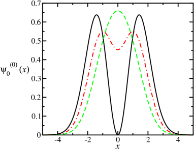
Figure 1: (Color online) Symmetric ground state wave function for $N=0$, $\psi_{0,2}^{(0)}(d)$, for three different values of the cutoff length $d=0,1,2$ (full black, dash-dotted red and dashed green lines correspondingly).

The 1-RDM takes the form

$$\rho_{0,2}^{(0)}(x,y)\,=\,\frac{e^{-(x^{2}+y^{2})/2}}{4\,\sqrt{\pi}\,(3+4d^{2}+4d^{4})}(3+8d^{2}+16d^{4}+2(1+4d^{2})(x^{2}+y^{2})+8xy+4x^{2}y^{2})\,.$$ (20)

Using the orthonormal Hermite functions

$$\psi_{k}(x)\,=\,\frac{e^{-\frac{1}{2}x^{2}}\,H_{k}(x)}{\sqrt{2^{k}k!\pi^{1/2}}}\,,$$ (21)

where $H_{k}(x)$ are the Hermite polynomials, the $1$-RDM can be written as

$$\rho^{(0)}_{0,2}({x};{y})\,=\,\sum_{i,j=0}^{2}\,\rho_{i,j}(d)\,\psi_{i}({x})\,\psi_{j}({y})\,.$$ (22)

The $1$-RDM above can be cast in matrix form

$$\left[\rho_{0,2}^{(0)}\right](d)\,=\,\left(\begin{array}[]{ccc}\frac{3/8+d^{2}+d^{4}}{3/4+d^{2}+d^{4}}&0&\frac{1+2d^{2}}{4\sqrt{2}(3/4+d^{2}+d^{4})}\\ 0&\frac{1}{4(3/4+d^{2}+d^{4})}&0\\ \frac{1+2d^{2}}{4\sqrt{2}(3/4+d^{2}+d^{4})}&0&\frac{1}{8(3/4+d^{2}+d^{4})}\end{array}\right)\,,$$ (23)

and its eigenvalues can be exactly calculated and are given by

$$\lambda_{\pm} = \frac{2+4d^{2}+4d^{4}\pm(1+2d^{2})\sqrt{3+4d^{2}+4d^{4}}}{2(3+4d^{2}+4d^{4})}$$

$$\lambda_{o} = \frac{1}{4(3/4+d^{2}+d^{4})}\,.$$ (24b)

These eigenvalues are showed in Fig. 2. In the important limit $d\rightarrow 0$ we obtain

$$\left[\rho_{0,2}^{(0)}\right](0)\,=\,\left(\begin{array}[]{ccc}\frac{1}{2}&0&\frac{1}{3\sqrt{2}}\\ 0&\frac{1}{3}&0\\ \frac{1}{3\sqrt{2}}&0&\frac{1}{6}\end{array}\right)\,,$$ (25)

whose eigenvalues are

$$\lambda_{\pm}\,=\,\frac{2\pm\sqrt{3}}{6}\;;\;\lambda_{o}\,=\,\frac{1}{3}\,,$$ (26)

as reported in Ref. opos15 . For $d\rightarrow\infty$, replacing $g_{2}^{(0)}(d)$ in Eq. (1), the interaction potential becomes a constant, and the 1-RDM correspond to two non-interacting harmonic particles in the ground state,

$$\lim_{d\rightarrow\infty}\left[\rho_{0,2}^{(0)}\right](d)\,=\,\left(\begin{array}[]{ccc}1&0&0\\ 0&0&0\\ 0&0&0\end{array}\right)\,.$$ (27)

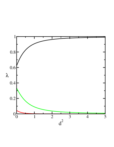
Figure 2: (Color online) Eigenvalues of the $N=0$ reduced density matrix for symmetric solutions, $\rho^{(0)}_{0,2}(d)$ (Eq. (20)), as a function of the squared cutoff length $d^{2}$.

III.2 N=1

In this case $k_{N}^{2}=9$, which implies $E_{N}=5$. The value for $v_{1}$ is

$$v_{1}(d,g)\,=\,1+4d^{2}-\frac{g}{2}\,,$$ (28)

and the condition $v_{2}=0$ gives

$$g_{\pm}\,=\,7+6d^{2}\pm\sqrt{25-12d^{2}+4d^{4}}\,.$$ (29)

Performing the same analysis for the functions $g_{\pm}(d)$ as was done previously for $g_{2}^{(0)}(d)$, we get that $g_{+}(d=0)=12\Rightarrow p=4\Rightarrow g_{+}(d)=g^{(1)}_{4}(d)$, and similarly $g_{-}(d)=g^{(1)}_{2}(d)$. Then, Eq. (17) gives two solutions for the energy, $E_{0,4}$, corresponding to the ground state for $g=12$, and $E_{2,2}$ corresponding to the second excited state for $g=2$. $g^{(1)}_{4}$ corresponds to the ground state, with the nodeless wave function

$$\psi_{0,4}^{(1)}(x)\,=\,\frac{2\sqrt{2}\left(2d^{4}+d^{2}(7-2d^{2}+D)x^{2}+(5-2d^{2}+D)x^{4}\right)e^{-x^{2}/2}}{\pi^{1/4}\sqrt{525(5+D)+2d^{2}\left(60+75D+2d^{2}\left(2d^{2}(8+6d^{2}-D)-3(8+D)\right)\right)}}\;.$$ (30)

where $D=\sqrt{25+4(d^{2}-3)d^{2}}$. The limit cases of this wave function for $d\rightarrow 0$ and $d\rightarrow\infty$ are

$$\left.\psi_{0,4}^{(1)}(x)\right|_{d=0}\,=\,\frac{4x^{4}e^{-x^{2}/2}}{\pi^{1/4}\sqrt{105}}\;\;\;;\;\;\;\left.\psi_{0,4}^{(1)}(x)\right|_{d\rightarrow\infty}\,=\,\frac{e^{-x^{2}/2}}{\pi^{1/4}}\;,$$ (31)

the first one correspond to the Calogero ground state for $g=12$, the second one to the ground state of two non interacting particles in an harmonic potential. The 1-RDM is a $5\times 5$ matrix.

Taking $g^{(1)}_{2}$ we obtain the second excited state, whose wave function is

$$\psi_{2,2}^{(1)}(x)\,=\,\frac{2\sqrt{2}\left(2d^{4}+d^{2}(-7+2d^{2}+D)x^{2}+(5-2d^{2}-D)x^{4}\right)e^{-x^{2}/2}}{\pi^{1/4}\sqrt{-525(-5+D)+2d^{2}\left(60-75D+2d^{2}\left(2d^{2}(8+6d^{2}+D)+3(-8+D)\right)\right)}}\;,$$ (32)

which has two nodes. The limit of this wave function for $d\rightarrow 0$ is

$$\left.\psi_{2,2}^{(1)}(x)\right|_{d=0}\,=\,\frac{\sqrt{2}}{\sqrt{15}\pi^{1/4}}x^{2}(2x^{2}-5)e^{-x^{2}/2}\,,$$ (33)

which corresponds to the second excited state for the Calogero model with $g=2$, and for the limit $d\rightarrow\infty$ is

$$\left.\psi_{2,2}^{(1)}(x)\right|_{d\rightarrow\infty}\,=\,\frac{H_{2}(x)e^{-x^{2}/2}}{2\sqrt{2}\pi^{1/4}}\;.$$ (34)

The complete wave function is given by

$$\left.\psi(x_{1},x_{2})\right|_{d\rightarrow\infty}\,=\,\Psi(X)\,\left.\psi_{2,2}^{(1)}(x)\right|_{d\rightarrow\infty}\,=\,\frac{1}{2}\left(\psi_{2}(x_{1})\,\psi_{0}(x_{2})+\psi_{0}(x_{1})\,\psi_{2}(x_{2})\right)-\frac{1}{\sqrt{2}}\psi_{1}(x_{1})\,\psi_{1}(x_{2})\;,$$ (35)

note that these three terms are the only products of Hermite functions that give the energy $E=5$ and they share equal probability amongst even and odd eigenfunctions.

IV Antisymmetric eigenfunctions with N=0

The energy in this case is $k_{N}^{2}=7$ or $E_{N}=4$, and the condition $v_{1}=0$ gives

$$g^{(0)}_{3}=6+4d^{2}\,,$$ (36)

then, from Eq.(17), it correspond to the antisymmetric ground state $E_{0,3}$ where the reduced density matrix of the Calogero model is exactly solved for fermions opos15 . The reduced wave function is

$$\psi_{0,3}^{(0)}(x)\,=\,\frac{2\sqrt{2}x(d^{2}+x^{2})}{\pi^{1/4}\sqrt{15+12d^{2}+4d^{4}}}e^{-x^{2}/2}\,.$$ (37)

The 1-RDM takes the form

$$\rho_{0,3}^{(0)}(x,y)\,=\,\frac{e^{-(x^{2}+y^{2})/2}}{\pi^{1/2}8\left(15+12d^{2}+4d^{4}\right)} \left(15+24d^{2}+16d^{4}+(54+48d^{2}+32d^{4})xy\right.$$ (38)

$$+ 6(3+4d^{2})(x^{2}+y^{2})+4(3+4d^{2})xy(x^{2}+y^{2})$$

$$+ \left.36x^{2}y^{2}+8x^{3}y^{3}\right)\,.$$

The complete matrix in the Hermite basis set, Eq. (21), is

$$\left[\rho^{(0)}_{0,3}\right](d)\,=\,\left(\begin{array}[]{cccc}\frac{21+24d^{2}+8d^{4}}{4(15+12d^{2}+4d^{4})}&0&\frac{3\sqrt{2}(3+2d^{2})}{4(15+12d^{2}+4d^{4})}&0\\ 0&\frac{27+24d^{2}+8d^{4}}{4(15+12d^{2}+4d^{4})}&0&\frac{\sqrt{6}(3+2d^{2})}{4(15+12d^{2}+4d^{4})}\\ \frac{3\sqrt{2}(3+2d^{2})}{4(15+12d^{2}+4d^{4})}&0&\frac{9}{4(15+12d^{2}+4d^{4})}&0\\ 0&\frac{\sqrt{6}(3+2d^{2})}{4(15+12d^{2}+4d^{4})}&0&\frac{3}{4(15+12d^{2}+4d^{4})}\end{array}\right)\,,$$ (39)

and its eigenvalues, shown in Fig. 3, are

$$\lambda_{\pm}\,=\,\frac{1}{4}\left[1\pm\frac{\sqrt{2(99+4d^{2}(3+d^{2})(15+2d^{2}(3+d^{2}))}}{(15+2d^{2}(3+d^{2}))}\right]\;,\\$$ (40)

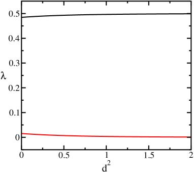
Figure 3: (Color online) Eigenvalues of the $N=0$ reduced density matrix for antisymmetric solutions, $\rho^{(0)}_{0,3}$ (Eq.(38)), as a function of the squared cutoff length $d^{2}$. Note that both eigenvalues are doubly degenerate.

both with multiplicity 2. In the limit $d\rightarrow 0$ we obtain the expressions reported for the two-fermion Calogero model opos15

$$\left[\rho^{(0)}_{0,3}\right](0)\,=\,\left(\begin{array}[]{cccc}\frac{7}{20}&0&\frac{3}{10\sqrt{2}}&0\\ 0&\frac{9}{20}&0&\frac{1}{10}\sqrt{\frac{3}{2}}\\ \frac{3}{10\sqrt{2}}&0&\frac{3}{20}&0\\ 0&\frac{1}{10}\sqrt{\frac{3}{2}}&0&\frac{1}{20}\end{array}\right)\,,$$ (41)

whose eigenvalues are

$$\lambda_{\pm}\,=\,\frac{5\pm\sqrt{22}}{20}\,.$$ (42)

For the limit $d\rightarrow\infty$ we get

$$\lim_{d\rightarrow\infty}\left[\rho^{(0)}_{0,3}\right](d)\,=\,\left(\begin{array}[]{cccc}\frac{1}{2}&0&0&0\\ 0&\frac{1}{2}&0&0\\ 0&0&0&0\\ 0&0&0&0\end{array}\right)\,,$$ (43)

V The Rényi and von Neumann entropies

So far, we have been involved with the quasi-exactly solvable aspect of the regularized Calogero model. This Section is devoted to analyze both the behavior of the entanglement entropies for the exact polynomial solutions and for arbitrary pairs of the pair $(g,d)$.

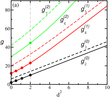
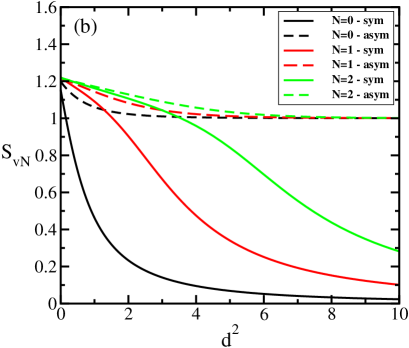
Figure 4: (Color online) (a) Isoenergetic curves $g^{(N)}_{p}(d)$ where an exact polynomial solution of the one-dimensional regularized Calogero model is known. From bottom to top the solid (dashed) lines correspond to symmetric (antisymmetric) ground-state wave functions for $N=0,1,2$. The brown dash-dotted line corresponds to $d^{2}=2$ used to compute the approximate eigenvalues of Fig. 5 (a) and the circles on this line are those shown at the bottom of the same figure and pinpoint the $g$ values for which a number of eigenvalues of the approximate $1$-RDM become null. Correspondingly, dots on the $g^{(0)}_{2}(d^{2})$ and $g^{(1)}_{4}(d^{2})$ symmetric curves correspond to those shown at the bottom of Fig. 6. (b) Exact von Neumann entropy of the ground-state wave functions obtained for the isoenergetic curves $g^{(N)}_{p}(d)$. The same color code is used in both panels.

For a given density matrix $\rho$ with an entanglement spectrum $\{\lambda_{i}\}$, its spectral decomposition is

$$\rho=\sum_{i}\lambda_{i}\left|{\phi_{i}}\right\rangle\left\langle\phi_{i}\right|,$$ (44)

where the $\left|{\phi_{i}}\right\rangle$’s are the eigenvectors or natural orbitals of $\rho$. The eigenvalues $\{\lambda_{i}\}$ are also known as natural occupation numbers.

The Rényi entropy of $\rho$ is defined as

$$S^{a}(\rho)=\frac{1}{1-a}\log_{2}\mbox{Tr}\rho^{a},$$ (45)

where $a>0$ is a constant (here we use $a$ instead of the more common $\alpha$ parameter to avoid possible conflicts with the parameter of Eq. (9)). Besides, it is well known that

$$\lim_{a\rightarrow 1}S^{a}(\rho)=S_{vN}(\rho)=-\mbox{Tr}(\rho\log_{2}\rho),$$ (46)

where $S_{vN}(\rho)$ is the von Neumann entropy. In some cases, the mono-parametric family of Rényi entropies shed more light over the peculiarities of the entanglement spectrum, i.e. the spectrum of the $\rho$ under study, because of its ability to weight differently the eigenvalues of $\rho$ by changing the value of $a$. This is made clear by looking at the expressions of both entropies, Eqs. (45) and (46), in terms of the eigenvalues of $\rho$

$$S^{a}(\rho)=\frac{1}{1-a}\log_{2}\left(\sum_{i}\lambda_{i}^{a}\right),\qquad S_{vN}=-\sum_{i}\lambda_{i}\log_{2}\lambda_{i}.$$ (47)

Let us start by inspecting the isoenergetic $g^{(N)}_{p}(d)$ curves in the $(g,d^{2})$ plane. Figure 4(b) show these curves for all the ground states $n=0$. Note that the curves hit the ordinate axis at the $g$ values where an exact polynomial solution of the Calogero model can be found opos15 . The von Neumann entropies (vNE) along each isoenergetic curve are presented in Fig. 4(a). The vNE for the symmetric case goes to zero for large values of the cutoff length parameter indicating a single natural orbital population. Conversely, in the antisymmetric case the vNE converges to a limiting value of one because the antisymmetrization prevents such single natural orbital population. Note that the vNE at $d=0$ is not the same for all curves and whether symmetric or antisymmetric configurations have larger vNE depends upon the particular $g^{(N)}_{p}(0)$ value as shown in opos15 for the Calogero model.

We turn now to the study of the $1$-RDM eigenvalues and vNE for arbitrary values of the parameters in the $(d^{2},g)$-plane. Figure 5(a) shows the typical behavior of the largest eigenvalues of the $1$-RDM for $d\neq 0$ as a function of $g$. The eigenvalues were calculated using a high precision variational method with a symmetrical Hermite-DVR basis set function Manthe2017 ; Beck2000 , so the eigenvalues corresponds to a symmetric problem. The method to obtain the eigenvalues of the 1-RDM from the approximate two-particle variational wave function has been discussed elsewhere Osenda2007 ; Osenda2008 ; Giesbertz2013 . There is a discrete set of $g$ values where a number of eigenvalues become null. From these points the eigenvalues are increasing functions of $g$, but only the two largest do not become null again. The rest reach some maximum and then become decreasing functions of $g$. After they go to zero, the two major eigenvalues do not become null again and so on.

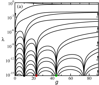
Figure 5: (Color online) (a) Approximate eigenvalues of the $1$-RDM as a function of $g$. The $1$-RDM was obtained from the variational wave function approximation to the symmetric ground state wave function for $d^{2}=2$. The coloured dots at the bottom indicate the $g$ values for which a number of eigenvalues become null, and are also indicated in Fig. 4(a). (b) Approximate von Neumann entropy corresponding to the eigenvalues shown in panel (a).

The values of $g$ where a number of eigenvalues become null for a given fixed value of $d$ can be plotted in the plane $(d^{2},g)$. Figure 4(a) shows these values for $d^{2}=2$ as filled dots and they match those shown at the bottom of Fig. 5(a). It is clear that the values of $g$ where a number of eigenvalues become null coincide with those found in the previous Sections, since the curves shown in Fig. 4(a) correspond to the analytical equations found for the lowest eigenvalues corresponding to symmetric and antisymmetric functions, see Eqs. (18),(29) y (36). Let us remember that the curves are isoenergetic, since the corresponding eigenvalue does not depend on $g$ or $d$ over the curve. Besides, the number of non-zero natural occupation numbers over each curve is always the same, and coincides with the number found in Sections III and IV. From bottom to top in Fig. 4(a) the number is equal to three, five, and so on, for the symmetric eigenvalues. The same can be said for the eigenvalues corresponding to the antisymmetric eigenfunctions.

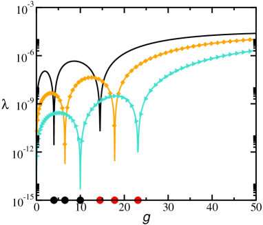
Figure 6: (Color online) 7th eigenvalue obtained from the $1$-RDM constructed from the variational approximation to the symmetric ground state wave function. The curves are for three values of the squared cutoff length $d^{2}=0.5,1.125,2$ (black, red and green correspondingly). The dots on the bottom indicate the interaction values $g$ for which the eigenvalue shows a behavior that resembles that of an almost vanishing eigenvalue. Those points are the same shown in Fig. 4(b) over the isoenergetic curves $g^{(0)}_{2}(d^{2})$ and $g^{(1)}_{4}(d^{2})$ for symmetric solutions.

Since the isoenergetic curves $g^{(N)}_{p}=g^{(N)}_{p}(d^{2})$ are increasing functions of $d^{2}$, it is clear that the values of $g$ where a number of eigenvalues become null are also increasing functions of $d$. This can be appreciated in Figure 6 where the seventh eigenvalue of the 1-RDM of the symmetric two-particle wave function is shown for several values of $d$. The sixth and seventh eigenvalues are the largest eigenvalues that have only two zeros. If $\lambda_{i}$ is the i-th eigenvalue of the 1-RDM, and $g_{n}^{i}$ is the $n$-th value of $g$ such that $\lambda_{i}(g_{n}^{i})=0$, then $g^{i}_{n}<g^{i}_{n+1}$ and $g^{i}_{n}(d_{1})<g^{i}_{n}(d_{2})$, $\forall\;d_{1}<d_{2}$.

The Rényi entropies also provide a way to identify models where the number of eigenvalues of the RDM that are different from zero alternates between infinity and a finite value. This is the case of the Calogero model for which it has been shown that the entanglement spectrum has a numerable infinite number of non-zero elements for open sets of the interaction parameter, besides these open sets are separated between them by a discrete set of values of the interaction parameter, $g_{n}$, where the number of non-zero eigenvalues of the entanglement spectrum is finite Garagiola2016 . As has been shown above, for the regularized Calogero model the set of values of the parameter where the entanglement spectrum is finite depends on the actual value of $d$, so $g_{n}=g_{n}(d)$.

The eigenvalues of the 1-RDM, at a fixed value of $d$, are analytical functions of $g$, and this can be exploited to assume a concrete analytical expression for the eigenvalues. As a consequence, explicit expressions for the Renyi entropies and its derivatives can be written. We develop here the case for symmetric two-particle wave function (the anti-symmetric case is similar), where the 1-RDM has only $2n+1$ non-zero eigenvalues at $g=g_{n}$, in the following the dependency with $d$ is dropped to keep the notation as simple as possible.

The following results will only rely on the analyticity of the eigenvalues around isolated points in the parameter space where the spectrum is finite. Assuming that

$$\lambda_{i}(g)\sim\left\{\begin{array}[]{lll}\lambda_{i}(g_{n})+\lambda_{i}^{(1)}(g-g_{n})&\mbox{ if }\;i\leq 2n+1\\ \mbox{}&\hskip 113.81102pt\mbox{ for }g\rightarrow g_{n}\\ \lambda_{i}^{(2)}(g-g_{n})^{2k_{i,n}}&\mbox{ if }i>2n+1\,,\end{array}\right.$$ (48)

where $\lambda_{i}^{(1)},\lambda_{i}^{(2)}$ are constants, and $k_{i,n}\geq 1$ is an integer. Eq. (47) can be written as

$$S^{a}(\nu) = \frac{1}{1-a}\,\log_{2}{\left(\sum_{i=1}^{2n+1}\lambda_{i}^{a}(g)+{\sum_{i=2n+2}^{\infty}\lambda_{i}^{a}(g)}\right)}$$

$$= \frac{1}{1-a}\,\left(\log_{2}{\left(\sum\limits_{i=1}^{2n+1}\lambda_{i}^{a}(g)\right)}+\log_{2}{\left(1+\frac{\sum\limits_{i=2n+2}^{\infty}\lambda_{i}^{a}(g)}{\sum\limits_{i=1}^{2n+1}\lambda_{i}^{a}(g)}\right)}\right)$$

$$\underset{g\rightarrow g_{n}}{\sim} \frac{1}{1-a}\,\left(\log_{2}{\left(\sum\limits_{i=1}^{2n+1}\lambda_{i}^{a}(g)\right)}+\frac{\sum\limits_{i=2n+2}^{\infty}\lambda_{i}^{a}(g)}{\ln{2}\,\sum\limits_{i=1}^{2n+1}\lambda_{i}^{a}(g)}\right)\,=\,S_{n}^{a}(g)+s_{n}^{a}(g)\,.$$

The last line of the equation above is the definition of the quantities $S_{n}^{a}(g)$ and $s_{n}^{a}(g)$. So, it is clear that $S_{n}^{a}(g_{n})=S^{a}(g_{n})$, and $s_{n}^{a}(g_{n})=0$. Then, the derivative of the Rényi entropy at $g=g_{n}$ can be obtained as

$$\left.\frac{\partial S^{a}(g)}{\partial g}\right|_{g=g_{n}} = \left.\frac{\partial S_{n}^{a}(g)}{\partial g}\right|_{g=g_{n}}+$$ (50)

$$\frac{a}{\ln{2}\,(1-a)}\,\left(\frac{\sum\limits_{i=2n+2}^{\infty}\lambda_{i}^{a-1}(g)\partial_{g}\lambda_{i}(g)}{\sum\limits_{i=1}^{2n+1}\lambda_{i}^{a}(g)}-\frac{\sum\limits_{i=2n+2}^{\infty}\lambda_{i}^{a}(g)\sum\limits_{i=1}^{2n+1}\lambda_{i}^{a-1}(g)\partial_{g}\lambda_{i}(g)}{\left(\sum\limits_{i=1}^{2n+1}\lambda_{i}^{a}(g)\right)^{2}}\right)_{g=g_{n}}\,.$$

The first term in Eq. (50) is a well-defined constant and the third one is zero. As a result of this, the derivative is dominated by the second term. Using the analytic expansion of the eigenvalues, Eq. (48), and assuming that $k_{m}$ is the minimum value of $k_{i,n}$, the leading asymptotic behavior of $s_{n}^{a}$ is

$$s_{n}^{a}(g)\underset{g\rightarrow g_{n}}{\sim}C_{n}\,((g-g_{n})^{2k_{m}})^{a}\,=\,C_{n}\,|g-g_{n}|^{\chi k_{m}}\,,$$ (51)

where $\chi=2a$, which implies that

$$\frac{\partial s_{n}^{a}(g)}{\partial g}\,\underset{g\rightarrow g_{n}}{\sim}\chi k_{m}C_{n}\,|g-g_{n}|^{\chi k_{m}-1}\,sign(g-g_{n})\,.$$ (52)

Collecting the results of the last few equations, the derivative of the Rényi entropy can be expressed as

$$\left.\frac{\partial S^{a}(g)}{\partial g}\right|_{g=g_{n}}\,=\,\left\{\begin{array}[]{lrl}\left.\begin{array}[]{lll}-sign(C_{n})\times\infty&\mbox{for }&g\rightarrow g_{n}^{-}\\ sign(C_{n})\times\infty&\mbox{for }&g\rightarrow g_{n}^{+}\end{array}\right\}&\mbox{if }\;\chi k_{m}<1\\ \left.\begin{array}[]{lrl}\partial_{g}S_{n}^{a}(g_{n})\,-C&\mbox{for }&g\rightarrow g_{n}^{-}\\ \partial_{g}S_{n}^{a}(g_{n})\,+C&\mbox{for }&g\rightarrow g_{n}^{+}\end{array}\right\}&\mbox{if }\;\chi k_{m}=1\\ \partial_{g}S_{n}^{a}(g_{n})&\mbox{if }\;\chi k_{m}\geq 1\,.\end{array}\right.$$ (53)

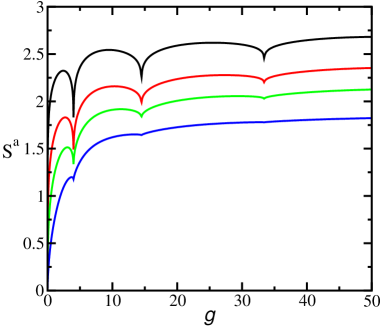
Figure 7: (Color online) Rényi entropies as a function of the interaction parameter $g$ for a cutoff length $d^{2}=0.5$. The parameter values $a=0.1,0.15,0.2,0.3$ (black, red, green and blue line correspondingly) were chosen. The kinks are located at $g$ values for which there is an exact polynomial expansion of the $1$-RDM, which renders a finite Hilbert space and hence many eigenvalues vanish. As shown in the text, the kinks are a consequence of the analyticity of the vanishing eigenvalues around those $g$ values.

Even tough the derivative of $S^{a}$ is continuous for $\chi\geq 1$, it is straightforward to see from the eigenvalue asymptotics, Eq. (48), that the second derivative diverges for $1<\chi k_{m}<2$, but it is analytical for $\chi k_{m}=2$, i.e the kink at $\chi k_{m}=1$ is smoothed until it disappears at $\chi k_{m}=2$.

Figure 7 shows the behavior of $S^{a}$ for different values of the parameter $a$, as a function of $g$, while $d=$ is kept fixed. The kinks at fixed values of $g$ can be easily appreciated, as well as their softening for increasing values of $a$ as predicted by Eq. (53), observe that the bottom curve corresponds to the largest value of $a$ depicted while the upper curve corresponds to the lower one. Keeping $d$ fixed assures that the points $g_{m}$ where only a number of eigenvalues are non-zero are also kept fixed and, as a consequence, the kinks in the curves calculated for different values of $a$ are located at the same abscissas.

VI discussion

Few particle models with exact and finite reduced density matrices are even more scarce than models with exact solutions, making them valuable examples to test numerical methods to obtain the spectrum of the Hamiltonian and the entanglement spectrum. Recently, there has been a number of works dealing with the properties of the entanglement spectrum, or natural occupation numbers, in particular the phenomenon of pinning. Much of the understanding has been obtained analyzing systems of coupled harmonic oscillators (or Moshinsky model), because they are amenable of a complete analytical treatment. It is feasible that the study of quasi-solvable models helps the efforts made to understand the pinning phenomenon and other related issues.

Quasi-exactly solvable models have wave functions that are polynomial functions on the inter-particle distance so, at least for those that do not depend on any angular variable but the ones on the inter-particle radius, they should also possess exact and finite reduced density matrices. This last problem is open for three dimensional problems with non-trivial angular momentum.

For the model analyzed in this work, the quasi-exactly solvable character is intertwined with the fact that the Calogero model has exact solutions that can be expressed as polynomials in the interparticle distance. So, when we take the limit $d\rightarrow 0$ over the isoenergetic lines we are able to recover all the quantities corresponding to the Calogero model. Then, it is natural to wonder if a given quasi-solvable model has always, in some limit, an unknown exactly solvable relative.

The Rényi entropy shows, again, that it is a capable tool to identify systems with exact and finite RDM. Nevertheless, to improve its usability it is necessary to determine if a set of very small eigenvalues are effectively zero or not. To accomplish this it is necessary to identify if, for example, performing a finite size analysis of the numerical eigenvalues at the parameter where the system has an exact and finite RDM the behaviour is (quite) different from the behavior where there is not such a RDM. It is clear that for models with wave functions with only a polynomial dependency on the inter-particle distance it is possible to choose a finite basis set that expands the Hilbert space where the wave function to be analyzed is contained exactly, resulting in an exact RDM. In this case, the RDM derived from the finite basis contains all the information required to produce a finite number of non-zero eigenvalues and a number of exactly zero ones. Conversely, when the finite basis set used to analyze a given wave function does not contain the exact wave function under consideration there will be a number of eigenvalues that should be zero in the limit of an infinite basis set, but for a finite basis they are not and a numerical criterion is in order. Work around these lines is in progress.

References

- (1) F. Calogero, J. Math. Phys. 10, 2191 (1969).
- (2) H. Azuma and S. Iso, Phys. Lett. B 331, 107 (1994).
- (3) B. D. Simons, P. A. Lee, and B. L. Altshuler, Phys. Rev. Lett. 70, 4122 (1993).
- (4) A. P. Polychronakos, Phys. Rev. Lett. 70, 2329 (1993).
- (5) A. Gorsky and N. Nekrasov, Nucl. Phys. B 414, 213 (1994).
- (6) O. Chalykh, M. Feigin, and A. Veselov, J. Math. Phys. 39, 695 (1998).
- (7) F. Atai and E. Langmann, J. Math. Phys. 58, 011902 (2017).
- (8) A. P. Polychronakos, Nucl. Phys. B 543, 485 (1999).
- (9) M. Znojil and M. Tater, J. Phys. A: Math.Gen. 34, 1793 (2001).
- (10) C.A. Downing, Phys. Rev. A 95, 022105 (2017).
- (11) B. Sutherland, J. Math. Phys. 12, 246 (1971).
- (12) O. Osenda, F. Pont, A. Okopińska, and P. Serra, J. Phys. A: Math. Gen. 48, 485301 (2015).
- (13) M. Garagiola, E. Cuestas, F. M. Pont, P. Serra, and O. Osenda, Phys. Rev. A 94, 042115 (2016).
- (14) H.Katsura and Y. Hatsuda, J. Phys. A: Math. Theor. 40, 13931 (2007).
- (15) A.G Ushveridze, Quasi-Exactly Solvable Models in Quantum Mechanics (Institute of Physics, Bristol, 1994).
- (16) G. S. Ezra and R. S. Berry, Phys. Rev. A 25, 1513 (1982).
- (17) G. S. Ezra and R. S. Berry, Phys. Rev. A 28, 1989 (1983).
- (18) P.-F. Loos and Peter M. W. Gill, Phys. Rev. Lett. 103, 123008 (2009).
- (19) A. Alavi, J. Chem. Phys. 113, 7735 (2000).
- (20) S. Ghosh and P. M. W. Gill, J. Chem. Phys. 122, 154108 (2005).
- (21) I. G. Ryabinkin and V. N. Staroverov, Phys. Rev. A 81, 032509 (2010).
- (22) J. Jung, P. Garcia-Gonzalez, J. E. Alvarellos, and R. W. Godby, Phys. Rev. A 69, 052501 (2004).
- (23) P.-F. Loos, C. J. Ball, and P. M.W. Gill, J. Chem. Phys. 140, 18A524 (2014).
- (24) P.-F. Loos, Phys. Rev. A 89, 052523 (2014).
- (25) J. Jung and J. E. Alvarellos, J. Chem. Phys. 118, 10825 (2003).
- (26) P.-F. Loos, Phys. Rev. A 81, 032510 (2010).
- (27) V. Tognetti, and P.-F. Loos, J. Chem. Phys. 144, 054108 (2016).
- (28) C. A. Downing, J. Math. Phys. 54, 072101 (2013).
- (29) C. A. Downing, and M. E. Portnoi, Phys. Rev. B 94, 045430 (2016).
- (30) S. Kais, D. R. Herschbach, and R. D. Levine, J. Chem. Phys. 91, 7791 (1989).
- (31) M. Taut, Phys. Rev. A 48, 3561 (1993).
- (32) A. Ronveaux, editor, Heun’s Differential Equations (Oxford University Press, Oxford, U.K., 1995).
- (33) P.P. Fiziev, J. Phys. A: Math. Gen. 43, 035203 (2010).
- (34) K.A. Motsepe, M.Y. Shatalov and S.V. Joubert, Appl. Math. Comput. 239, 47–55 (2014).
- (35) P. P. Fiziev and D. R. Staicova, Phys. Rev. D 84, 127502 (2011).
- (36) P. P. Fiziev, D. R. Staicova, arxiv:1201.0017.
- (37) L. G. Jiao, L. R. Zan, Y. Z. Zhang, and Y. K. Ho, Int. J. Quantum Chem. 117, e25375 (2017).
- (38) U. Manthe, J. of Phys.: Condens. Matt. 29, 253001 (2017).
- (39) M. H. Beck, A. Jäckle, G. A. Worth, and H.-D. Meyer, Phys. Rep. 324, 1 (2000).
- (40) O. Osenda and P. Serra, Phys. Rev. A 75, 042331 (2007).
- (41) O. Osenda, P. Serra and S. Kais, Int. J. Quantum Inf. 6, 303 (2008).
- (42) K. J. H. Giesbertz and R. van Leeuwen, J. Chem. Phys. 139, 104109 (2013).