Efficient approximation of functions of some large matrices by partial fraction expansions

Abstract

Some important applicative problems require the evaluation of functions $\Psi$ of large and sparse and/or localized matrices $A$. Popular and interesting techniques for computing $\Psi(A)$ and $\Psi(A)\mathbf{v}$, where $\mathbf{v}$ is a vector, are based on partial fraction expansions. However, some of these techniques require solving several linear systems whose matrices differ from $A$ by a complex multiple of the identity matrix $I$ for computing $\Psi(A)\mathbf{v}$ or require inverting sequences of matrices with the same characteristics for computing $\Psi(A)$. Here we study the use and the convergence of a recent technique for generating sequences of incomplete factorizations of matrices in order to face with both these issues. The solution of the sequences of linear systems and approximate matrix inversions above can be computed efficiently provided that $A^{-1}$ shows certain decay properties. These strategies have good parallel potentialities.

Our claims are confirmed by numerical tests.

65F60, 65F08, 15A23

1 Introduction

The numerical evaluation of a function $\Psi(A)\in{\mathbb{C}}^{n\times n}$ of a matrix $A\in{\mathbb{C}}^{n\times n}$ is ubiquitous in models for applied sciences. Functions of matrices are involved in the solution of ordinary, partial and fractional differential equations, systems of coupled differential equations, hybrid differential-algebraic problems, equilibrium problems, complex networks, in quantum theory, in statistical mechanics, queuing networks, and many others. Motivated by the variety of applications, important advances in the development of numerical algorithms for matrix function evaluations have been presented over the years and a rich literature is devoted to this subject; see, e.g., [39, 33, 24, 23] and references therein.

In this paper we focus mainly on functions of large and sparse and/or localized matrices $A$. A typical example of localized matrix generated by a PDE, say, is the one whose nonnegligible entries are concentrated in a small region within the computational domain showing a rapid decay away from this region. Localization often offers a way to perform (even full) matrix computations much more efficiently, possibly with a linear cost with respect to the degrees of freedom. For a very interesting treatment on this new point of view we suggest the review [5]. In the latter there are also several examples of localized matrices from physics, Markov chains, electronic structure computations, graph, network analysis, quantum information theory and many others.

For the computation of $\Psi(A)$ with $A$ as above, the available literature offers few efficient strategies. The existing numerical methods for computing matrix functions can be broadly divided into three classes: those employing approximations of $\Psi$, those based on similarity transformations of $A$ and matrix iterations. When the size $n$ of the matrix argument $A$ is very large, as for example when it stems from a fine grid discretization of a differential operator, similarity transformations and matrix iterations can sometimes be not feasible since their computational cost can be of the order of $n^{3}$ flops in general. To overcome these difficulties we consider an efficient computational framework for approximation algorithms based on partial fraction expansions. In particular, let us consider an approximation of $\Psi(A)$ of the form

$$f(A)=\sum_{j=1}^{N}c_{j}(\xi_{j}I-A)^{-1}$$ (1)

where scalars $c_{j}$ and $\xi_{j}$ can be complex and $I$ is the $n\times n$ identity matrix. The above approach has been proven to be effective for a wide set of functions $\Psi$.

In general, computing (1) requires inverting several complex valued matrices and, with the exception of lucky or trivial cases, if $n$ is large, this can be computationally expensive. We propose to overcome this issue by approximating directly each term $(\xi_{j}I-A)^{-1}$ with an efficient update of an inexact sparse factorization inspired by the complex valued preconditioners update proposed in [10] that there was defined for symmetric matrices $A$ only. Moreover, such strategy can be extended to the computation of the action of the matrix function on vectors, that is, to compute $\Psi(A)\mathbf{v}$ for a given vector $\mathbf{v}$. Vectors of this form often represent the solution of important problems. The simplest example is the vector $\exp(t_{1}A)\mathbf{y}_{0}$ which represents the solution at a time $t_{1}$ of the differential equation $\mathbf{y}^{\prime}(t)=A\mathbf{y}(t)$ subject to the initial condition $\mathbf{y}(t_{0})=\mathbf{y}_{0}$.

Note that if the interest is just on obtaining the vector $\Psi(A)\mathbf{v}$ and not $\Psi(A)$, then ad hoc strategies can be applied as, for example, well known Krylov subspace methods [39, 25] and [35, 42, 38, 1, 29, 36, 34, 22] and others.

The paper is organized as follows: in Section 2 we recall the basics of matrix functions, together with some results on approximation theory to ground the proposed approach. Section 3 recalls a recent updating strategy we propose to use in the algorithms to approximate matrix functions. In Section 4 the proposed approximation for matrix functions is analyzed by first recalling some recent results on our updating process for approximate inverse factorizations and then using the underlying results to build an a-priori bound for the error made. Section 5 is devoted to numerical tests showing the effectiveness of the approach in a variety of applications and comparisons. Section 6 discusses briefly some final issues.

2 Computing function of matrices by partial fraction expansions

Many different definitions have been proposed over the years for matrix functions. We refer to N. Higham [24] for an introduction and references.

In this work we make use of a definition based on the Cauchy integral: given a closed contour $\Gamma$ lying in the region of analiticity of $\Psi$ and enclosing the spectrum of $A$, $\Psi(A)$ is defined as

$$\Psi(A)=\frac{1}{2\pi i}\int_{\Gamma}\Psi(z)(zI-A)^{-1}dz.$$ (2)

Thus, any analytic function $\Psi$ admits an approximation of the form (1). Indeed, the application of any quadrature rule with $N$ points on the contour $\Gamma$, leads to an approximation as in (1).

In [23] authors address the choice of the conformal maps to deal with the contour $\Gamma$ for special functions like $A^{\alpha}$ and $\log(A)$ when $A$ is a real symmetric matrix whose eigenvalues lie in an interval $[a,b]\subset(0,\infty)$. The basic idea therein is to approximate the integral in (2) by means of the trapezoidal rule applied to a circle in the right half–plane surrounding $[a,b]$. Thus,

$$\Psi(A)\approx f(A)=\gamma A\operatorname{Im}\displaystyle\sum_{j=1}^{N}c_{j}(\xi_{j}I-A)^{-1}$$ (3)

where $\gamma$ depends on $a,b$ and a complete elliptic integral, while the $\xi_{j}$ and $c_{j}$ involve Jacobi elliptic functions evaluated in $N$ equally spaced quadrature nodes. We refer to [23] for the implementation details and we make use of their results for our numerical tests. In particular, an error analysis is presented there and we report here briefly only the main result; see [23].

Theorem 2.1.

Let $A$ be a real matrix with eigenvalues in $[a,b]\,,0<a<b$, let $\Psi$ be a function analytic in ${\mathbb{C}}\backslash(-\infty,0]$ and let $f(A)$ be the approximation in (3). Then

$$\|\Psi(A)-f(A)\|={\cal{O}}(e^{-{\pi}^{2}N/(\log(b/a)+3)}).$$

The analysis in [23] also applies to matrices with complex eigenvalues.

An approximation like (1) can also derive from a rational approximation $R_{N}$ to $\Psi$, given by the ratio of two polynomials of degree $N$, with the denominator having simple poles. A popular example is the Chebyshev rational approximation for the exponential function on the real line. This has been largely used over the years and it is still a widely used approach, since it guarantees an accurate result even for low degree $N$, say $N=16$. Its poles and residues are listed in [17] while in [16] the approximation error is analyzed and the following useful estimate is given

$$\sup_{x\geq 0}|\exp(-x)-R_{N}(x)|\approx 10^{-N}.$$

Another example is the diagonal Padé approximation to the logarithm, namely

$$\log(I+A)\approx f(A)=\displaystyle A\sum_{j=1}^{N}\alpha_{j}(I+\beta_{j}A)^{-1};$$ (4)

this is the core of the logm$\_$pade$\_$pf code in the package by Higham [24] and we will use it in our numerical tests in Section 5. Unfortunately, as for every Padé approximant, formula (4) works accurately only when $\|A\|$ is relatively small, otherwise scaling-and-squaring techniques or similar need to be applied. The error analysis for the matrix case reduces to the scalar one, according to the following result; see [28].

Theorem 2.2.

If $\|A\|<1$ and $f(A)$ is defined as (4) then

$$\|\log(I+A)-f(A)\|\leq|f(-\|A\|)-\log(1-\|A\|)|.$$

In some important application, the approximation of the matrix $\Psi(A)$ is not required and it is enough to get the vector $\Psi(A)\mathbf{v}$ for a given vector $\mathbf{v}$. In this case, by using (1), we formally get the approximation

$$f(A)\mathbf{v}=\sum_{j=1}^{N}c_{j}(\xi_{j}I-A)^{-1}\mathbf{v}$$ (5)

which requires to evaluate $(\xi_{j}I-A)^{-1}$ or $(\xi_{j}I-A)^{-1}\mathbf{v}$ for several values of $\xi_{j}$, $j=1,\ldots,N$. Usually, if $A$ is large and sparse or localized or even structured, the matrix inversions in (5) should be avoided since each term $\mathbf{w}_{j}\equiv(\xi_{j}I-A)^{-1}\mathbf{v}$ is mathematically (but fortunately not computationally) equivalent to the solution of the algebraic linear system

$$(\xi_{j}I-A)\ \mathbf{w}_{j}=\ \mathbf{v}.$$ (6)

3 Updating the approximate inverse factorizations

In the underlying case of interest, i.e., $A$ large and sparse and/or localized or structured, solving (6) by standard direct algorithms can be unfeasible and in general a preconditioned iterative framework is preferable. However, even using an iterative solver but computing $N$ preconditioners, one for each of the matrices $(A+\xi_{j}I)$, can be expensive. At the same time, keeping the same preconditioner for all the $N$ linear systems (see, e.g., [38]), even if chosen appropriately, may not account for all the possible issues. Indeed, very different order of magnitude of the complex valued parameters $\xi_{j}$ can cause potential risks for divergence of the iterative linear system solver. Our proposal is based on cheap updates for incomplete factorizations developed during the last decade started by the papers [6] and [10] essentially based on the inversion and sparsification of a reference approximation used to build updates. We stress that the updates in [6] and [10] were studied for symmetric matrices. In recent years these algorithms have been generalized towards either updates from any symmetric matrix to any other symmetric (see [14]) and nonsymmetric matrices (see [2, 3], and [11]) with applications to very different contexts, but still little attention has been spent on the update of incomplete factorizations for sequences of nonsymmetric linear systems with a complex shift.

Among the strategies that can provide a factorization for the inverse of $A$ we consider the approximate inverses or AINV by Benzi et al. (see [4] and references therein) and the inversion and sparsification proposed by van Duin [43], or INVT for short. Both the approaches are very interesting, and differ slightly in their computational cost (see [13] for some recent results), parallel potentialities and stability.

Several efforts have been done in the last decade in order to update the above mentioned incomplete factorizations in inverse form, usually as preconditioners; see [6, 10, 14, 3, 11].

Here, in order to build up an approximate factorization (or, better saying, to approximate an incomplete factorization) for each factor $(\xi I-A)^{-1}$, as $\xi$ varies, we assume that $A$ can be formally decomposed as $A=L\,\,D\,U^{H}$ with $L$, $U$ lower triangular matrices and that the factorization is well defined. Then, the inverse of $-A$ can be formally decomposed as

$$-A^{-1}=U^{-H}D^{-1}L^{-1}=ZD^{-1}W^{H},$$

where $W=L^{-H}$ and $Z=U^{-H}$ are upper triangular with all ones on the main diagonal and $D$ is a diagonal matrix, respectively. The process can be based also on different decompositions but here we focus on LDU-types only. In general, this is a not practical way to proceed because the factors $L$ and $U$ (and thus their inverses) are often dense. At this point we have two possibilities. The first is use AINV and its variants (again see [4]) that provides directly an approximate inverse in factored form for $A$ whose factors can be suitably sparse as well if $A$ is sparse or shows certain decay properties. The second is use an inversion and sparsification process as in [43], that, starting from a sparse incomplete factorization for $A$ such as ILU (see, e.g., [40]) $P=\tilde{L}\tilde{D}\tilde{U}^{H}$ approximating $A$, whose factors $\tilde{L}$, $\tilde{U}$ are sparse, produces an efficient inversion of $\tilde{L}$, $\tilde{U}$ and provides also a post-sparsification of the factors $Z$ and $W$ to get $\tilde{Z}$ and $\tilde{W}$. A popular post-sparsification strategy can be to zero all the entries smaller than a given value and/or outside a prescribed pattern. We call seed preconditioner, denoted $P_{0}$, the following approximate decomposition of $A^{-1}$:

$$P_{0}=\tilde{Z}\,\tilde{D}^{-1}\,\tilde{W}^{H}.$$ (7)

Similarly to what done above for $A^{-1}$, in the style of [10], given a complex pole $\xi$, a factorization for the inverse of the complex nonsymmetric matrices in (6) can be formally obtained by the identities

$$A_{\xi}^{-1} \equiv (-A+\xi\,I)^{-1}$$

$$= (W^{-H}\,D\,Z^{-1}+\xi\,W^{-H}(W^{H}\,Z)Z^{-1})^{-1}$$

$$= Z\,\left(D+\xi\,E\right)^{-1}W^{H},\quad E=W^{H}\,Z.$$

However, as recalled above, the factors $Z$ and $W$ are dense in general. Therefore, their computation and storage are sometimes possible for $n$ small to moderate but can be too expensive to be feasible for $n$ large. This issue can be faced by using the sparse approximations $\tilde{Z}$ and $\tilde{W}$ for $Z$ and $W$, respectively, produced by AINV, by inversion and sparsification or by another process generating a sparse factorization for $A^{-1}$. Indeed, supposing that the chosen algorithm generates a well defined factorization, we can provide an approximate factorization for the inverse of $A+\xi_{j}I$. In particular, we get a sequence of approximate factorization candidates using $P_{0}$ defined above as a reference and $\tilde{E}$, a sparsification of the nonsymmetric real valued matrix $E$, with the approximation of $A_{\xi}^{-1}$ given by $P_{\xi}$ defined as

$$P_{\xi}=\tilde{Z}\,\left(\tilde{D}+\xi\tilde{E}\right)^{-1}\tilde{W}^{H},$$ (9)

where, by using the formalism introduced in [3],

$$\tilde{E}=g(\tilde{W}^{H}\,\,\tilde{Z}).$$ (10)

The function $g$ serves to generate a sparse matrix from a full one such that the linear systems with matrix $\tilde{D}+\xi\tilde{E}$ can be solved with a low computational complexity, e.g., possibly linear in $n$. As an example, if the entries of $A^{-1}$ decay fast away from the main diagonal, we can consider the sparsifying function $g=g_{m}$,

$$g_{m}:\mathbb{C}^{n\times n}\rightarrow\mathbb{C}^{n\times n},$$

extracting $m$ upper and lower bands (with respect to the main diagonal, which is the $0$-diagonal) of its matrix argument generating an $(2m,2m)$–banded matrix. In general, a matrix $A$ is called $m$-banded if there is an index $l$ such that

$$a_{i,j}=0,\;\;\text{ if }j\notin[i-l,i-l+m].$$

It is said to be centered and $m$-banded if $m$ is even and the $l$ above can be chosen to be $m/2$. In this case the zero elements of the centered and $(m,m)$-banded are:

$$a_{i,j}=0,\;\;\text{ if }|i-j|>\frac{m}{2},$$

thus selfadjoint matrices are naturally centered, i.e., a tridiagonal selfadjoint matrix is centered and $2$-banded. This choice will be used in our numerical examples but of course different choices for $g$ can be more appropriate in different contexts. A substantial saving can be made by approximating

$$g_{m}(\tilde{W}^{H}\,\,\tilde{Z})\textrm{ with }g_{m}(\tilde{W}^{H})\,g_{m}(\,\tilde{Z}),\quad m>0$$

with a reasonable quality of the approximation, i.e., under suitable conditions and provided $m>0$, the relative error

$$\frac{||g_{m}(\tilde{W}^{H}\,\,\tilde{Z})-g_{m}(\tilde{W}^{H})\,g_{m}(\,\tilde{Z})||}{||\tilde{W}^{H}\,\,\tilde{Z}||}$$

can be moderate in a way that will be detailed in Theorem 4.3 discussed in the next section.

4 Analysis of the approximation processes

We use here the underlying approximate inverses in factored form (9) as a preconditioner for Krylov solvers to approximate $\Psi(A)\mathbf{v}$ and to approximate $f(A)$ by

$$\tilde{f}(A)= \displaystyle\sum_{j=1}^{N}c_{j}P_{\xi_{j}}$$ (11)

$$= \displaystyle\sum_{j=1}^{N}c_{j}\tilde{Z}\,\left(\tilde{D}+\xi_{j}\tilde{E}\right)^{-1}\tilde{W}^{H}.$$

In order to discuss an a-priori bound for the norm of the error $||\Psi(A)-\tilde{f}(A)||$ generated by the various approximation processes, supposing we are operating in exact arithmetic, we need some results on the update of the approximate inverse factorizations.

Let us recall a couple of results that can be derived as corollaries of Theorem 4.1 in [20]. In this context, we consider a general complex, separable, Hilbert space $H$, and denote with $\mathcal{B}(H)$ the Banach algebra of all linear operators on $H$ that are also bounded. If $A\in\mathcal{B}(H)$, then $A$ can be represented by matrix with respect to any complete orthonormal set thus $A$ can be regarded as an element of $B(l^{2}(S))$, a matrix representing a bounded operator in $\mathcal{B}(l^{2}(S))$, where $S=\{1,2,\ldots,N\}$.

Theorem 4.1.

Let $A\in\mathbb{C}^{n\times n}$ be a nonsingular $(2m,2m)$–banded matrix, with $A\in\mathcal{B}(l^{2}(S))$ and condition number $\kappa_{2}(A)\geq 2$. Then, by denoting with $b_{i,j}$ the ${i,j}-$entry of $A^{-1}$ and with

$$\beta=\left(\frac{\kappa_{2}(A)-1}{\kappa_{2}(A)+1}\right)^{\frac{1}{2m}},$$

for all $\tilde{\beta}>\beta$, $\tilde{\beta}<1$, there exists a constant $c>0$ such that

$$|b_{i,j}|\leq c\,\tilde{\beta}^{|i-j|},$$

with

$$\begin{split}c\leq&(2m+1)\frac{\kappa_{2}(A)+1}{\kappa_{2}(A)-1}\|A^{-1}\|\kappa_{2}(A)\\ \leq&3(2m+1)\|A^{-1}\|\kappa_{2}(A).\end{split}$$

For the proof and more details, see [12, Theorem 3.10].

We can note immediately that the results in Theorem 4.1, without suitable further assumptions, can be of very limited use because:

• the decay of the extradiagonal entries can be very slow, in principle arbitrarily slow;

• the constant $c$ in front of the bound depends on the condition number of $A$ and we are usually interested in approximations of $A^{-1}$ such that their condition numbers can range from moderate to high;

• the bound is far to be tight in general. A trivial example is given by a diagonal matrix with entries $a_{j,j}=j$, $j=1,\ldots,n$. We have that $b_{i,j}=0$, $i\neq j$ but of course $\kappa_{2}(A)=a_{n,n}/a_{1,1}=n$.

• If we take $m=n$ and $n$ is very large, then $\tilde{\beta}$ must be chosen very near $1$ and it is very likely that no decay can be perceptible with the bound in Theorem 4.1.

However, the issues presented here are more properly connected with the decay properties of the matrices $Z$, $W$ (and therefore $\tilde{Z}$, $\tilde{W}$). Using similar arguments as in Theorem 4.1 in [9], it is possible to state the following result.

Corollary 4.2.

Let $A\in\mathbb{C}^{n\times n}$ be invertible, $A\in\mathcal{B}(l^{2}(S))$, and with its symmetric part positive definite. Then for all $i$, $j$ with $j>i$, the entries $z_{i,j}$ in $Z=L^{-H}$ and $w_{i,j}$ in $W=U^{-1}$ satisfy the following upper bound:

$$|z_{i,j}|\leq c_{1}\,\tilde{\beta}_{1}^{j-i},\quad|w_{i,j}|\leq c_{2}\,\tilde{\beta}_{2}^{j-i},\quad j>i$$

(note that $z_{i,j}$, $w_{i,j}=0$ for $j\leq i$), where

$$0<\tilde{\beta}_{1},\ \tilde{\beta}_{2}\leq\tilde{\beta}<1$$

and $c_{1}$, $c_{2}$ are positive constants, $c_{1},c_{2}\leq c_{3}\cdot\kappa_{2}(A).$

Recently, this kind of decay bound for the inverses of matrices was intensely studied, and appears also with other structures. Consider, e.g., the case of nonsymmetric band matrices in [37], tridiagonal and block tridiagonal matrices in [32], triangular Toeplitz matrices coming from the discretization of integral equations [21], Kronecker sum of banded matrices [15], algebras with structured decay [27] and many others. Thus, the results we propose can be readily extended to the above mentioned cases.

If the seed matrix $A$ is, e.g., diagonally dominant, then the decay of the entries of $A^{-1}$ and therefore of $W$, $Z$ ($\tilde{W}$, $\tilde{Z}$) is faster and more evident. This can be very useful for at least two aspects:

• the factors $\tilde{W}$, $\tilde{Z}$ of the underlying approximate inverse in factored form can show a narrow band for drop tolerances even just slightly larger than zero;

• banded approximations can be used not only for post–sparsifying $\tilde{W}$, $\tilde{Z}$ in order to get more sparse factors, but also the update process can benefit from the fast decay.

Theorem 4.3.

Let $A\in\mathbb{C}^{n\times n}$ be invertible, $A\in\mathcal{B}(l^{2}(S))$, and with its symmetric part positive definite. Let $g_{m}=[\cdot]_{m}$ be a sparsifying function extracting the $m$ upper and lower bands of its argument. Then, given the matrices from Corollary 4.2, we have

$$[\tilde{W}^{H}\,\tilde{Z}]_{m}=[\tilde{W}^{H}]_{m}[\tilde{Z}]_{m}+R(A,m),$$

$$|(R(A,m))_{i,j}|\leq c_{4}\tilde{\beta}^{|i-j|},$$

where $c_{4}=c_{1}c_{2}$.

The above result can be proved by comparing the expressions of $\tilde{W}^{H}\tilde{Z}$ and $g_{m}(\tilde{W}^{H}\tilde{Z})$ and using Corollary 4.2 with an induction argument on $n$.

As a matter of fact, we see that a fast decay of entries of $A^{-1}$ guarantees that the essential component of the proposed update matrix, i.e., $\tilde{E}=\tilde{W}^{H}\tilde{Z}$, can be cheaply, easily and accurately approximated by the product $g_{m}(\tilde{W}^{H})\cdot g_{m}(\tilde{Z})$, without performing the time and memory consuming matrix-matrix product $\tilde{W}^{H}\tilde{Z}$.

On the other hand, if the decay of the entries of $A^{-1}$ is fast, even a simple diagonal approximation of $\tilde{W}^{H}\,\tilde{Z}$ can be accurate enough. In this case, there is no need to apply the approximation in Theorem 4.3. The update matrix $\tilde{E}$ can be produced explicitly by the exact expression of $\operatorname{diag}(\tilde{W}^{H}\,\tilde{Z})$ we give in the following corollary.

Corollary 4.4.

Let $A\in\mathbb{C}^{n\times n}$ be invertible, $A\in\mathcal{B}(l^{2}(S))$, and with its symmetric part $(2m,2m)$–banded and positive definite, $1\leq m\leq n$. Then, the diagonal approximation for $\tilde{E}$ generated by the main diagonal of $\tilde{W}^{H}\,\tilde{Z}$ is given by

$$\tilde{E}=\operatorname{diag}(\tilde{W}^{H}\,\tilde{Z})=(d_{i,i}),$$

where

$$d_{i,i}=1+\sum_{j=1,\ i-j\leq m}^{i-1}\tilde{w}_{j,i}\tilde{z}_{j,i},\quad 1\leq i\leq n,$$

where $\tilde{w}_{j,i}$ and $z_{j,i}$ are the entries of $\tilde{W}$ and $\tilde{Z}$, respectively.

All our numerical experiments use the approximations proposed in Theorem 4.3 and in Corollary 4.4 without perceptible loss of accuracy; see Section 5.

We use the properties stated by the previous results to get an a–priori estimates of the global error $\|\psi(A)-\tilde{f}(A)\|$ that is given below in exact arithmetics and for $A$ symmetric and definite positive in order to use the results in [23]. Note that, with the above hypotheses, we get $\tilde{Z}=\tilde{W}$ in (11) and therefore

$$\tilde{f}(A)=\sum_{j=1}^{N}c_{j}\tilde{Z}\,\left(\tilde{D}+\xi_{j}\tilde{E}\right)^{-1}\tilde{Z}^{H}.$$ (12)

Theorem 4.5.

Let $A$ be a real positive definite matrix with eigenvalues in $[a,b]$, $0<a<b$, $\Psi$ a function analytic in ${\mathbb{C}}\backslash(-\infty,0]$, $f(A)$ the approximation of $\psi(A)$ in (3) and $\tilde{f}(A)$ the approximation of $f(A)$ in (9) with $0<\tau<1$ drop tolerance used to produce $\tilde{Z}$. Moreover, let $\Delta_{Z}=\tilde{Z}-Z$. Then,

$$\|\psi(A)-\tilde{f}(A)\|\leq E_{1}(N)+E_{2}(\tau),$$

with

$$E_{2}(\tau)=c(\beta)\,\tau=O(||\Delta_{Z}||),$$

where $c=c(\beta)$ is a parameter that depends on the decay of the offdiagonal entries of $Z$, and

$$E_{1}(N)={\cal{O}}(e^{-{\pi}^{2}N/(\log(b/a)+3)}).$$

The above result follows by observing that

$$\|\psi(A)-\tilde{f}(A)\|= \|\psi(A)-f(A)+f(A)-\tilde{f}(A)\|$$ (13)

$$\leq \|\psi(A)-f(A)\|+\|f(A)-\tilde{f}(A)\|.$$

The upper bound for the quadrature error $E_{1}(N)=\|\psi(A)-f(A)\|$ for an analytic function $\Psi$ is obtained straightforwardly from Theorem 2.1. Recall that the bound is derived from the classical error estimate for the Trapezoidal/Midpoint rule [18, Section 4.6.5]. Similar bounds for functions that are less smooth can be provided as well, even if they show just a polynomial decay, see again [18, Section 2.9].

The upper bound for the errors generated by the approximation of the terms $(A+\xi I)^{-1}$ by the approximate inverse factorization updates, i.e., $E_{1}(N)=\|f(A)-\tilde{f}(A)\|$, is easily derived by working on the norm of the difference between (3) and (9) substituting to $\tilde{Z}$ the expression $\tilde{Z}=Z+\Delta_{Z}$ and to $(\tilde{D}+\xi\tilde{E})^{-1}$ the expression $(D+\xi E)^{-1}+\Delta_{D}$. The claim follows by observing that $||\Delta_{D}||$, $||\Delta_{Z}||$ can be bounded by $c(\beta)\,\tau$; see Theorem 4.1 and Corollary 4.2.

A generalization of Theorem 4.5 for nonsymmetric matrices $A$ can be given with similar arguments.

The main purpose of the a-priori upper bound in Theorem 4.5 should be intended as more qualitative than quantitative, for showing that the multiple approximation processes considered here for computing $\tilde{f}(A)$ converge, i.e., in exact arithmetic, under the hypotheses of Theorem 2.1, $\|\psi(A)-\tilde{f}(A)\|\rightarrow 0$ if $\tau\rightarrow 0$ and $N\rightarrow\infty$.

4.1 Cross-relations between the function $g$ and drop tolerance $\tau$

To clarify the role of the function $g$ introduced in (10) and the drop tolerance $\tau$ for AINV, we compare the results of our approach to compute $\exp(A)$ with the built–in Matlab function expm. We use the expression in (1) for the Chebyshev rational approximation of degree $N=16$ so that we can consider the approximation error negligible.

Consider the localized matrix $A=(A_{i,j})$ described in [8] with entries

$$A_{i,j}=\left\{\begin{array}[]{ll}e^{-\alpha(i-j)},&i\geq j,\\ e^{-\beta(j-i)}&i<j,\end{array}\right.\qquad\alpha,\beta>0.$$ (14)

This is typical example of a localized matrix, completely dense but with rapidly decaying entries. These matrices are usually replaced with banded matrices obtained by considering just few bands or by dropping entries which are smaller than a certain threshold. Here we sparsify it by keeping only $15$ off–diagonals on either side of its main diagonal. Let us take $\alpha=\beta=0.5$ and $\alpha=\beta=1.2$ for a small example, namely $50\times 50$, in order to show the application of Theorem 4.1. The approximation we refer to is (11), in which we let $\tau$ and $g$ change, with effects on the factors $\tilde{Z},\tilde{W}$ and $\tilde{E}$ in (10), respectively. The continuous curves in Figure 1 refer to the “exact” approach, that is, for $\tau=0$ leading to full factors $\tilde{W}$ and $\tilde{Z}$. In the abscissa we report the number of extra-diagonals selected by $g$. Notice that both $\tau$ and $g$ are important because even for $\tau=0$ more extra-diagonals are necessary to reach a high accuracy.

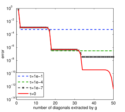
(a)

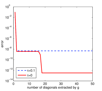
(b)

Figure 1: Behavior of the error for $\exp(A)$ as $\tau$ and $g$ vary. The $50\times 50$ matrix argument $A$ has the expression in (14) with $\alpha=\beta=0.5$ (left), $\alpha=\beta=1.2$ (right). The x-axis reports the number of diagonals the function $g$ selects while the y-axis reports the error with respect to the Matlab’s expm(A). AINV is used with the tolerance $\tau$ given in the figures’ caption.

From the plots in Figure 1, we note that the loss of information in discarding entries smaller than $\tau$ cannot be recovered even if $g$ extracts a full matrix. In the left plot, for a moderate decay in the off-diagonals entries, a conservative $\tau$ is necessary to keep the most important information. On the other hand, when the decay is more evident, as in the right plot, a large $\tau$ is enough, and $g$ keeping just two diagonals gives already a reasonable accuracy. We get similar results also for the logarithm, as well as for other input matrices.

4.2 Choosing the reference preconditioner(s)

To generate a viable update (9), we need to compute an appropriate seed preconditioner (7). Note that the poles $\xi_{j}$ in the partial fraction expansion (5) for the Chebyshev approximation of the exponential have a modulus that grows with the number of points; see, e.g., Figure 2.

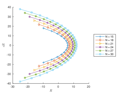
(a)

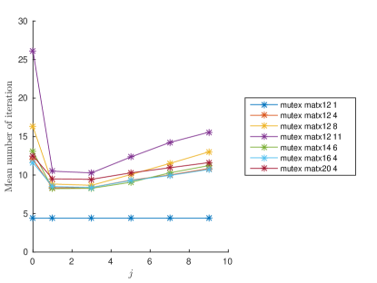
(b)

Figure 2: Position of the poles of Chebyshev approximation of $\exp$ (left) and a sample of mean number of iterations (right) for different choice of $P_{\text{seed}}$ for the mutual exclusion model from [41].

Therefore, we need to take into account the possibility that the resolvent matrices

$$(\xi_{j}I-A)^{-1},\quad j=1,\ldots,N$$

become diagonally dominant or very close to the identity matrix, up to a scalar factor, or, in general, with a spectrum that is far from the one of $-A$. Sometimes the matrices related to the resolvent above can be so well conditioned that the iterative solver does not need any preconditioner. In this case, any choice of the seed preconditioner as an approximate inverse of the matrix $-A$ is almost always a poor choice, and thus also the quality of the updates; see [6, 10]. Let us consider, e.g., the matrices from the mutual exclusion model from [41]. These are the transition matrices for a model of $M$ distinguishable process (or users) that share a resource, but only $M^{\prime}$, with $1\leq M^{\prime}\leq M$ that could use it at the same time. In Figure 2 (right) the underlying experiments are reported as “mutex matx$M$ $M^{\prime}$”. We report the mean iterations required when the $P_{\text{seed}}$ corresponding to $\xi_{j}$ is used for $j=1,\ldots,N$, while $j=0$ refers to the seed preconditioner for $-A$, all obtained with INVT for $\tau_{L}=1e-5$ and $\tau_{Z}=1e-2$. The plot clearly confirms that working with $-A$ is always the most expensive choice, while better results are obtained for whatever pole and sometimes the pole with the largest modulus slightly betters the others.

Observe also that in this way complex arithmetic should be used to build the approximate inverse of the matrix $(\xi_{1}I-A)$, because its main diagonal has complex valued entries.

5 Numerical tests

The codes are written in Matlab (R2016a). The machine used is a laptop running Linux with 8Gb memory and CPU Intel(R) Core(TM) i7-4710HQ CPU with clock 2.50GHz.

The sparse inversion algorithm chosen for each numerical test (those used here are described in Section 3) takes into account the choice made for the computation of the reference (or seed for short) preconditioners. If the matrix used to compute the seed preconditioner is real, we use the AINV. Otherwise, the inversion and sparsification of the ILUT Algorithm, or INVT for short, requiring a dual threshold strategy. See [13] for details and a revisitation of AINV and INVT techniques. In the following, the symbols $\tau$ denotes drop tolerance for AINV while $\tau_{L}$, $\tau_{Z}$ the threshold parameter for ILU decomposition and for post-sparsification of the inverted factors of INVT; respectively; see also the details discussed in Section 4.2. $\varepsilon_{\text{rel}}$ denotes the standard relative (to a reference solution) error.

Other details on the parameters and strategies used are given in the description of each experiment.

5.1 Approximating $\Psi(A)$

Let us focus on the approximation of $\exp(A)$ and $\log(A)$. In the following tables, the columns Update refers to the approximation (11). Columns Direct are based on the direct inversion of the matrices $(A+\xi_{j}I)^{-1}$ in (1).

The Fill–In for computing the incomplete factors approximating the underlying matrices is computed as

$$\text{Fill--In}\ =\frac{nnz(\tilde{Z})+nnz(\tilde{W})-n}{n^{2}},$$ (15)

where $n$ denotes the size and $nnz(\cdot)$ the number of the nonzero entries, as usual.

5.1.1 $\log(A)$ - Exponential Decay

We consider the evaluation of $\log(A)$ where the entries of $A$ are as in (14) with $\alpha=0.2$ and $\beta=0.5$ and $n$ varies from $500$ to $8000$. For this matrix we use a drop tolerance $\tau=0.1$ to get a sparse approximate inverse factorization of $A$ with AINV. The resulting factors $\tilde{Z}$ and $\tilde{W}$ are bidiagonal and thus we take $g(X)=X$. The inversion of the tridiagonal factors is the more demanding part of the Update technique. For this test, we compare the Update and Direct methods, based on the approximation (3), with the Matlab function logm and the logm$\_$pade$\_$pf code in the package by N. Higham [24].

Numerical tests on scalar problems show that the degree $N=5$ for the Padé approximation (4) and $N=7$ for the approximant in (3) allow to reach a similar accuracy with respect to the reference solution. Thus, we use these values for $N$ in our tests.

Table 1: Execution time in seconds for $\log(A)$ for $A$ as in (14) with $\alpha=0.2$ and $\beta=0.5$. AINV with $\tau=1e-1$ is used.

n	Update	Direct	logm	logm$\_$pade$\_$pf	Fill–In
500	1.53	1.33	13.05	0.67	6e-3
1000	4.90	4.69	44.40	3.31	3e-3
2000	12.23	13.86	407.28	38.67	1e-3
4000	37.04	56.23	6720.36	522.25	7e-4
8000	168.41	412.30	70244.41	6076.00	7e-4

Results in Table 1 show that, for small examples, the Update and the logm$\_$pade$\_$pf approaches require a similar execution time, while the efficiency of the former becomes more striking with respect to all the others as the problem dimension increases.

5.1.2 $\exp(A)$ - Exponential Decay

We now consider the error for the matrix exponential. The test matrix is symmetric as in (14) for three choices of the parameter $\alpha$. We analyze the error of the approximations provided by the Update and Direct methods, for the Chebychev rational approximation of degree $N=8$, with respect to the results obtained by the expm Matlab command. We consider $\alpha=\beta=1,\,\alpha=\beta=1.5,\,\alpha=\beta=6$. For the first two cases, the drop tolerance for the AINV is $\tau=0.1$ and $g=g_{1}(\cdot)$ extracts just the main diagonal and one superdiagonal. For the third case, AINV with $\tau=10^{-3}$ is used and $\tilde{Z},\,\tilde{W}$ are both diagonal. No matrix inversion is thus performed.

Table 2: Errors for the Update and Direct methods compared to the Matlab’s expm(A). The parameters are $\tau=0.1$, $\tilde{Z}$ and $\tilde{W}$ bidiagonal, for $\alpha=\beta=1$ (left) and $\alpha=\beta=1.5$ (center); $\alpha=\beta=6$. AINV is used with $\tau=10^{-3}$ and $\tilde{Z}$, $\tilde{W}$ are diagonal (right).

n	Update	Direct
500	1.1e-7	2.3e-8
1000	1.1e-7	2.3e-8
2000	1.1e-7	2.3e-8
4000	1.1e-7	2.3e-8

(a)

n	Update	Direct
500	2.3e-08	2.3e-08
1000	2.3e-08	2.3e-08
2000	2.3e-08	2.3e-08
4000	2.3e-08	2.3e-08

(b)

n	Update	Direct
500	4.5e-06	1.8e-08
1000	4.5e-06	1.8e-08
2000	4.5e-06	1.8e-08
4000	4.5e-06	1.8e-08

(c)

Results from Table 2 show the good accuracy the Update approach reaches. Indeed, although the presence of the sparsification errors (see the action of $\tau$ and $g$), the error is comparable with the one of the Direct method, which does not suffer from truncation. For the case $\alpha=\beta=6$, the difference between the two errors is more noticeable but it has to be balanced with great savings in timings. Indeed, in this case the decay of the off–diagonal entries of the inverse of $A$ is very fast and we exploit this feature by combining the effect of the small drop tolerance $\tau=10^{-3}$ and a function $g=g_{0}(\cdot)$ extracting just the main diagonal. Then, the computational cost is much smaller for the Update approach since no matrix inversion is explicitly performed and we experienced an overall linear cost in $n$, as in the other experiments. Thus, when a moderate accuracy is needed, the Update approach is preferable, since it is faster; see Table 3.

Table 3: Timings in seconds for $\exp(A)$ with $A$ as in (14) with $\alpha=\beta=6$. AINV with $\tau=10^{-3}$ is used and $g$ extracts just the main diagonal. The Fill–In column refers to the Fill–In occurred for computing the factors $\tilde{W}$ and $\tilde{Z}$ measured as in (15).

n	Update	Direct	expm	Fill–In
500	0.01	0.06	1.97	2.0e-3
1000	0.00	0.01	6.19	1.0e-3
2000	0.00	0.01	30.52	5.0e-4
4000	0.00	0.06	172.89	2.5e-4
8000	0.01	0.10	910.16	1.3e-4

5.1.3 $\exp(A)$ - Kronecker Structure

Now, let us test our approach in the context of the numerical solution of a 3D reaction–diffusion linear partial differential equation

$$\partial_{t}u=-k\nabla^{2}u+\gamma(x,y,z)u.$$ (16)

Discretizing (16) in the space variables with second order centered differences, the reference solution can be computed by means of the matrix $\exp(A)$. We take $k=1e-8$, and the action of $\gamma(x,y,z)$ is given by the matrix–vector product on the semidiscrete equation between $G=\operatorname{sparsify}(\operatorname{rand}(n^{3},n^{3}))$ where $n$ is the number of mesh points along one direction of the domain $\Omega=[0,1]^{3}$. Function $\operatorname{sparsify}$ gives a sparse version of $G$ with $0.1\%$ of fill–in and the Laplacian is discretized with the standard 7-points stencil with homogeneous Dirichlet conditions, i.e., the semidiscrete equation reads as

$$\mathbf{u}_{t}(t)=(A+G)\mathbf{u}(t).$$

The results of this experiment are reported in Table 4. The reference matrix is computed by using the incomplete inverse LDU factorization (INVT) that needs two drop tolerances, $\tau_{L}=1e-6$ and $\tau=\tau_{Z}=1e-8$. The former is the drop tolerance for the incomplete $LU$ (or $ILU$ for short) process and the latter for the post-sparsification of the inversion of $LU$ factors, respectively; see [13] for details on approximate inverse preconditioners with inversion of an $ILU$. A tridiagonal approximation of the correction matrix $\tilde{E}=\tilde{Z}^{T}\tilde{W}$ is used, i.e., $\tilde{E}=g_{1}(\tilde{Z}^{T}\tilde{W})$.

Table 4: Execution time in seconds for $\exp(A)$ and relative errors ($\varepsilon_{\text{rel}}$) with respect to expm(A) where $A$ is the discretization matrix of (16) (the time needed for building the reference matrix is not considered). INVT with $\tau_{L}=1e-6$ and $\tau=\tau_{Z}=1e-8$ is used.

	Direct		Update		expm$(A)$
$n^{3}$	T(s)	$\varepsilon_{\text{rel}}$	T(s)	$\varepsilon_{\text{rel}}$	T(s)	Fill-in
512	0.15	2.85e-07	0.07	2.82e-07	0.92	100.00 %
1000	0.83	2.85e-07	0.35	2.83e-07	8.19	100.00 %
1728	4.28	2.85e-07	0.94	2.83e-07	46.23	92.40 %
4096	118.39	2.85e-07	3.72	2.84e-07	669.39	51.77 %
8000	834.15	2.85e-07	9.69	2.82e-07	4943.73	28.84 %

5.2 Approximating $\Psi(A)\mathbf{v}$

5.2.1 $\exp(A)\mathbf{v}$ - Exponential Decay

To apply our approximation for $\Psi(A)\mathbf{v}$, where $A$ is large and/or localized and/or possibly structured, we use a Krylov iterative solver for the systems $(A+\xi_{j}I)\mathbf{x}=\mathbf{v}$ in (5) with and without preconditioning (the corresponding columns will be labeled as Prec and Not prec). The iterative solvers considered are BiCGSTAB and CG (the latter for symmetric matrices). The preconditioner is based on the matrix $\tilde{Z}(\tilde{D}+\xi_{j}\tilde{E})^{-1}\tilde{W}^{H}$ as in (9). The matrix $A$ has the entries as in (14) while $\mathbf{v}$ is the normalized unit vector.

Table 5: Iterates average and execution time in seconds for $\log(A)\mathbf{v}$ for $A$ as in (14) with $\alpha=0.2,\,\beta=0.5$. The linear systems are solved with the Matlab’s implementation of BiCGStab with and without preconditioning. INVT with $\tau=\tau_{L}=\tau_{Z}=1e-1$ is used.

	Prec		Not prec
n	iters	T(s)	iters	T(s)
500	2	0.05	21	0.11
1000	2	0.05	19	0.18
2000	2	0.08	18	0.33
4000	2	0.95	17	2.96

The average of the iterates in Table 5 is much smaller when the preconditioner is used. Moreover, preconditioned iterations are independent on the size of the problem.

In Table 6 we report the error, with respect to the Matlab’s expm(A)v, of the approximations given by the Prec and Not prec options. The entries in the test matrix have so a fast decay, since $\alpha=\beta=6$, that the term $\tilde{E}$ can be chosen diagonal. Interestingly, a good accuracy is reached with respect to the true solution. Moreover, the timings for the Prec approach is negligible with respect to that for the Not prec.

Table 6: Error for $\exp(A)\mathbf{v}$ for $A$ as in (14) with $\alpha=\beta=6$. Prec: our technique with $\tilde{E}$ diagonal. Not prec.: (5) when the linear systems are solved with the Matlab’s PCG used without preconditioning. INVT with $\tau=\tau_{L}=\tau_{Z}=1e-1$ is used.

n	Prec	Not prec
	$\varepsilon_{rel}$	$\varepsilon_{rel}$
500	4.5e-06	1.8e-08
1000	4.5e-06	1.8e-08
2000	4.5e-06	1.8e-08
4000	4.5e-06	1.8e-08

5.2.2 $\exp(A)\mathbf{v}$ - Transition Matrices

Let us consider a series of tests matrices of a different nature: the infinitesimal generators, i.e., transition rate matrices from the MARCA package by Stewart [41]. They are large non–symmetric ill–conditioned matrices whose condition number ranges from $10^{17}$ to $10^{21}$ and their eigenvalues are in the square in the complex plane given by $[-90,5.17e-15]\times i[-3.081,3.081]$. As a first example, we consider the NCD model. It consists of a set of terminals from which the same number of users issue commands to a system made by a central processing unit, a secondary memory device and a filling device. In Table 7 we report results for various $n$, obtained by changing the number of terminals/users. The matrices $A$ are used to compute $\exp(A)\mathbf{v}$, $\mathbf{v}=(1\ 2\ \ldots n)^{T}/n$. We compare the performance of BiCGSTAB for solving the linear systems in (5) without preconditioner and with our updating strategy, where $g$ extracts only the main diagonal, i.e., $g(\cdot)=g_{0}(\cdot)$. The INVT algorithm with $\tau_{Z}=1e-4$ and $\tau_{L}=1e-2$ is used to produce the approximate inverse factorization. The comparisons consider the time needed for solving each linear system, i.e., the global time needed to compute $\exp(A)\mathbf{v}$. Both methods are set to achieve a relative residual of $10^{-9}$ and the degree of the Chebyshev rational approximation is $N=9$. The column $\varepsilon_{\text{rel}}$ reports the relative error between our approximation and $\operatorname{expm}(A)\mathbf{v}$. For the case with the largest size $\operatorname{expm}$ gives “out of memory”error.

Table 7: Approximation of $\exp(A)v$, $A$ from NCD queuing network example. BiCGSTAB, $N=9$, tol$=1e-9$, INVT algorithm with $\tau_{Z}=1e-4$ and $\tau_{L}=1e-2$ is used. A $\dagger$ is reported on the $\varepsilon_{\text{rel}}$ when the $\operatorname{expm}$ gives out of memory error and no reference solution is available.

	Not prec		Update
n	iters	T (s)	iters	T (s)	$\varepsilon_{\text{rel}}$
286	7.50	7.62e-03	7.50	7.60e-03	8.73e-09
1771	17.60	2.95e-02	17.60	3.00e-02	3.46e-07
5456	29.00	1.15e-01	29.00	1.18e-01	5.23e-06
8436	34.50	2.44e-01	28.00	1.67e-01	1.50e-05
12341	43.10	3.39e-01	33.20	2.68e-01	3.87e-05
23426	64.30	9.66e-01	42.30	6.26e-01	$\dagger$

5.2.3 $\exp(A)\mathbf{v}$ - Network Adjacency Matrix

Let us compute $\exp(A)\mathbf{v}$ for the matrix TSOPF_FS_b9_c6 of dimension $14454$ coming from [19]. Results are reported in Table 8 and Figure 3. For this case we do not have a reference solution and then the error because MATLAB’s expm gives out of memory error. Instead, we consider the Euclidean norm of the difference of the solutions obtained for consecutive values of $N$ for $N=6,\ldots,30$. The other settings for the solver remain unchanged in order to evaluate the efficiency of the algorithm for the same level of accuracy, i.e., we are using again the INVT algorithm with $\tau_{Z}=1e-4$ and $\tau_{L}=1e-2$.

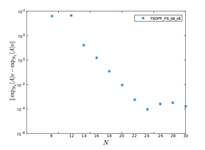
Figure 3: Accuracy for various values of $N$ for the TSOPF_FS_b9_c6 matrix

Table 8: Approximation of $\exp(A)v$ as the degree $N$ of the Chebyshev approximation varies. The matrix $A$ is TSOPF_FS_b9_c6 [19]. The INVT algorithm with $\tau_{Z}=1e-4$ and $\tau_{L}=1e-2$ is used.

Matrix TSOPF_FS_b9_c6
Size: 14454, $\kappa_{2}(A)=$3.1029e+12
Not prec		Prec
iters	T(s)	iters	T(s)	$N$
171.33	1.22e+00	15.00	2.62e-01	6
145.20	1.38e+00	36.50	1.05e+00	9
99.58	1.44e+00	8.75	2.33e-01	12
77.93	1.32e+00	7.64	2.29e-01	14
70.38	1.25e+00	7.06	2.44e-01	16
71.00	1.45e+00	6.61	2.65e-01	18
59.70	1.34e+00	6.15	2.80e-01	20
53.32	1.32e+00	5.95	2.93e-01	22
51.67	1.38e+00	5.75	3.14e-01	24
46.65	1.37e+00	5.58	3.30e-01	26
44.86	1.44e+00	5.39	3.49e-01	28
43.30	1.47e+00	5.20	3.66e-01	30

We observe two different effects for higher degree of approximations in Table 8. On one hand, from Figure 3, the relative error is reduced, as expected from the theoretical analysis, while, on the other, it makes the shifted linear system more well–conditioned. Note that the gain obtained using our preconditioning strategy is sensible even for large matrices.

5.2.4 $\log(A)\mathbf{v}$ - Polynomial Decay

Let us consider the matrix $A$ from [31] with entries given by

$$a_{i,j}=\frac{1}{2+(i-j)^{2}},\quad i,j=1,\ldots,n$$ (17)

in order to approximate $\log(A)\mathbf{v}$, $\mathbf{v}=(1,1,\ldots,1)^{T}$. $A$ is symmetric positive definite with a minimum eigenvalue of the order of $10^{-2}$ and its entries decay polynomially. We approximate $\log(A)\mathbf{v}$ with (5); BiCGSTAB is used with our preconditioner update strategy and without it (Not prec). The seed preconditioner is computed using INVT with $\tau_{Z}=1e-1$ and $\tau_{L}=1e-2$. We include the results with MATLAB’s $\operatorname{logm}(A)\mathbf{v}$. In particular, we use $N=30$ for the approximation of the logarithm function. Results are collected in Table 9.

Table 9: Computation of $\log(A)\mathbf{v}$ with $A$ as in equation (17). Note the moderate decay and a spectrum that ranges in the interval $[6e-2,3]$. For INVT $\tau_{Z}=1e-1$ and $\tau_{L}=1e-2$ are used.

BiCGSTAB	Not prec		Update			$\operatorname{logm}(A)\mathbf{v}$
n	iters	T(s)	iters	T(s)	Fill–In	T (s)	$\varepsilon_{\text{rel}}$
1000	11.88	2.4	5.07	1.25	3.16 %	0.169	1.91e-06
4000	11.05	34.2	4.73	16.8	0.80 %	14.7	1.54e-06
8000	10.58	133.78	4.53	65.7	0.40 %	116.9	1.66e-06
12000	10.32	296.9	4.38	145.7	0.27 %	428.2	1.74e-06

5.2.5 $\log(A)\mathbf{v}$ - Matrix Collection

Finally, we consider some matrices from The University of Florida Sparse Matrix Collection (see [19]), focusing on INVT with a seed preconditioner with $\tau_{Z}=1e-1$ and $\tau_{L}=1e-2$. The results are collected in Table 10, and confirm what we observed in the other tests.

Table 10: Approximation of $\log(A)\mathbf{v}$ with $A$ SPD from The University of Florida Sparse Matrix Collection. The real parts of the eigenvalues are all in the interval $[2.324e-14,1.273e+08]$. The updated preconditioners are computed using INVT with $\tau_{Z}=1e-1$ and $\tau_{L}=1e-2$.

BiCGSTAB		Not prec		Update			$\operatorname{logm}(A)\mathbf{v}$
Name	n	iters	T(s)	iters	T(s)	Fill–In	T(s)	$\varepsilon_{\text{rel}}$
1138_bus	1138	198.93	1.3	31.18	0.4	0.84 %	0.22	4.41e-07
Chem97ZtZ	2541	27.98	0.34	6.43	0.12	0.10 %	3.5	1.87e-07
bcsstk21	3600	157.85	4.8	76.4	3.1	1.36 %	10	3.10e-07
t2dal_e	4257	232.00	4.2	98.90	1.78	0.02 %	2.58	6.82e-04
crystm01	4875	23.35	1.03	11.48	0.56	0.17 %	25.3	3.16e-07

5.3 $\Psi(A)\mathbf{v}$ with updates and with Krylov subspace methods

A popular class of effective algorithms for approximating $\Psi(A)\mathbf{v}$ for a given large and sparse matrix $A$ relies on Krylov subspace methods. The basic idea is to project the problem into a smaller space and then to make its solution potentially cheaper. The favorable computational and approximation properties have made the Krylov subspace methods extensively used; see, e.g., [39, 30, 25, 34].

Over the years, some tricks have been added to these techniques to make them more effective, both in terms of computational cost and memory requirements, see, e.g., [35, 42, 38, 1, 29, 36]. In particular, as shown by Hochbruck and Lubich [25], the convergence depends on the spectrum of $A$. For our test matrices the spectrum has just a moderate extension in the complex plane. Thus, the underlying Krylov subspace techniques for approximating $\Psi(A)\mathbf{v}$ can be appropriate.

The approximation spaces for these techniques are defined as

$${\cal{K}}_{m}(A,\mathbf{v})={\textrm{span}}\{\mathbf{v},A\mathbf{v},\ldots,A^{m-1}\mathbf{v}\}.$$

Since the basis given by the vectors $\mathbf{v}=\mathbf{v}_{1},A\mathbf{v}=\mathbf{v}_{2},\ldots,A^{m-1}\mathbf{v}=\mathbf{v}_{m}$ can be very ill–conditioned, one usually applies the modified Gram-Schmidt method to get an orthonormal basis with starting vector $\mathbf{v}_{1}=\mathbf{v}/\|\mathbf{v}\|$. Thus, if these vectors $\mathbf{v}_{1},\ldots,\mathbf{v}_{m}$ are the columns of a matrix $V_{m}$ and the upper Hessenberg matrix $H_{m}$ collects the coefficients $h_{i,j}$ of the orthonormalization process, the following expression by Arnoldi holds

$$AV_{m}=V_{m}H_{m}+h_{m+1,m}\mathbf{v}_{m+1}\mathbf{e}_{m}^{T},$$

where $\mathbf{e}_{m}$ denotes the $m$th column of the identity matrix. An approximation to $\Psi(A)\mathbf{v}$ can be obtained as

$$y_{m}=\|\mathbf{v}\|V_{m}\Psi(H_{m})\mathbf{e}_{1}.$$

The procedure reduces to the three-term Lanczos recurrence when $A$ is symmetric, which results in a tridiagonal matrix $H_{m}$. One has still to face the issue of evaluating a matrix function, but, if $m\ll n$, for the matrix $H_{m}$, which is just $m\times m$. Several approaches can then be tried. For example, one can use the built–in function $\tt{funm}$ in Matlab, based on the Schur decomposition of the matrix argument, and the Schur-Parlett algorithm to evaluate the function of the triangular factor [24].

We consider the application of our strategy for the computation of $\exp(A)\mathbf{v}$, with a matrix $A$ generated from the discretization of the following 2D advection-diffusion problem

$$\left\{\begin{array}[]{rl}u_{t}=&\displaystyle\frac{\partial}{\partial x}\left(k_{1}\frac{\partial u}{\partial x}\right)+\frac{\partial}{\partial y}\left(k_{2}(y)\frac{\partial u}{\partial y}\right)\\ &\displaystyle+t_{1}(x)\frac{\partial u}{\partial x}+t_{2}(y)\frac{\partial u}{\partial y},\quad x\in[0,1]^{2}\\ u(x,y,t)=&0,\quad x\in\partial[0,1]^{2},\\ u(x,y,0)=&u_{0}(x,y)\end{array}\right.$$ (18)

where the coefficients are $k_{1}=10^{-2}$, $k_{2}(x)=2+10^{-5}\cos(5\pi x)$, $t_{1}(x)=1+0.15\sin(10\pi x)$ and $t_{2}(x)=1+0.45\sin(20\pi x)$. The second order centered differences and first order upwind are used to discretize the Laplacian and the convection terms, respectively. The purpose of this experiment, whose results are in Table 11, is comparing the performance of our updating approach, using INVT with $\tau_{L}=1e-5$ and $\tau_{Z}=1e-2$, with a Krylov subspace method. For the latter we use the classical stopping criterion based on monitoring

$$\gamma=h_{m+1,m}|\mathbf{e}_{m}^{T}\exp(H_{m})\mathbf{e}_{1}|.$$

We stop the iteration when $\gamma$ becomes smaller than $10^{-6}$. The threshold $\gamma$ was tuned to the accuracy expected by the Update approach.

Table 11: Errors and execution time for $\exp(A)\mathbf{v}$ for $A$ obtained as the finite difference discretization of (18). INVT with $\tau_{L}=1e-5$ and $\tau_{Z}=1e-2$ is used.

n	Update		Arnoldi
	$\varepsilon_{\text{rel}}$	T(s)	$\varepsilon_{\text{rel}}$	T(s)
100	2.64e-06	6.74e-02	3.51e-06	2.91e-02
196	3.81e-06	7.80e-02	1.20e-06	1.09e-01
484	1.22e-08	2.97e-01	1.60e-08	5.23e-01
961	7.68e-07	1.27e+00	1.68e-07	2.70e+00

From these experiences and other non reported here, we can conclude that our techniques, under appropriate hypotheses of sparsity or locality of the matrices, seem to have reasonably comparable performances with Krylov methods when computing $\Psi(A)\mathbf{v}$.

Moreover, we can expect even more interesting performances when simultaneous computations of vectors such as $\Psi(A)\mathbf{w}_{1},\Psi(A)\mathbf{w}_{2},\ldots,\Psi(A)\mathbf{w}_{K}$ are required. This will give us another level of parallelism beyond the one that can be exploited in the simultaneous computation of the terms in (5). In particular, this can be true when $K$ is large and each vector $\mathbf{w}_{j}$ does depend on the previous values $\mathbf{w}_{i}$ and $\Psi(A)\mathbf{w}_{i}$. In this setting we can construct the factors once in order to reduce the impact of the initial cost for computing the approximate inverse factors. A building cost that can be greatly reduced by using appropriate parallel algorithms and architectures; see [13] and references therein.

6 Conclusions

Consider the hypotheses used in this research:

• the function $\Psi$ should be smooth enough in the sense of [23];

• the off–diagonal entries of $A^{-1}$ should decay fast enough away from the main diagonal.

A natural question arises: which is the most relevant feature to make our Update approach effective? Several papers have been devoted to the analysis of the decay of the entries of $\Psi(A)$ when the behavior of the entries of $A$ is known [20, 7, 26, 8]. A unifying analysis has been proposed in [8], where the influence of $A$ and $\Psi$ is considered. One of their results shows that the entries in $\Psi(A)$ can be bounded by a constant and a term depending on the decay of the entries of $A^{-1}$, provided that $\Psi$ is analytic in a suitable region containing the spectrum of $A$.

As an example, let us recall a result concerning band matrices (see [8, Corollary 3.6]). If $A$ is a diagonalizable band matrix of dimension $n\times n$, then we have

$$|\Psi(A)_{i,j}|<c\,\kappa_{2}(X)\lambda^{|i-j|},\,\,i,j=1\ldots,n$$

where $X$ is the matrix of eigenvectors of $A$, $\kappa(\cdot)$ is the condition number in the Euclidean norm, $c$ is a positive constant and $0<\lambda<1$. We suppose that $\kappa_{2}(X)$ is moderate, otherwise the above bound is useless.

The latter bound seems to give a slightly greater importance to the matrix argument $A$ than to the function $\Psi$.

This discussion confirms our experience: the performances of the Update approach seem to depend more on $A$ (in particular, on the behavior of the entries of $A^{-1}$ away from the main diagonal) than on $\Psi$. Indeed, as can be observed in Table 2, if we approximate $\exp(A)$, for three different matrix arguments with different decays, the accuracy changes seem to be more influenced by the matrix argument. A similar comment can be done also for the plots in Figure 1.

Funding

This work was supported in part by INDAM-GNCS 2018 projects “Tecniche innovative per problemi di algebra lineare” and “Risoluzione numerica di equazioni di evoluzione integrali e differenziali con memoria”.

References

- [1] M. Afanasjew, M. Eiermann, O.G. Ernst, and S. Guettel, Implementation of a restarted Krylov subspace method for the evaluation of matrix functions., Linear Algebra Appl. 429 (2008), pp. 2293–2314.
- [2] S. Bellavia, D. Bertaccini, and B. Morini, Quasi Matrix Free Preconditioners in Optimization and Nonlinear Least-Squares, in Numerical analysis and applied mathematics, T. Simos, ed., Vol. 1281, Uppsala, July 2009. AIP, 2010, pp. 1036–1039.
- [3] S. Bellavia, D. Bertaccini, and B. Morini, Nonsymmetric preconditioner updates in Newton–Krylov methods for nonlinear systems, SIAM J. Sci. Comput. 33 (2011), pp. 2595–2619.
- [4] M. Benzi, Preconditioning techniques for large linear systems: A survey, Journal of Computational Physics 182 (2002), pp. 418–477.
- [5] M. Benzi, Localization in matrix computations: Theory and applications, in Exploiting Hidden Structure in Matrix Computations: Algorithms and Applications, Springer, 2016, pp. 211–317.
- [6] M. Benzi and D. Bertaccini, Approximate inverse preconditioning for shifted linear systems, BIT, Numerical Mathematics 43 (2003), pp. 231–244.
- [7] M. Benzi and G.H. Golub, Bounds for the entries of matrix functions with applications to preconditioning, BIT 39 (1999), pp. 417–438.
- [8] M. Benzi and N. Razouk, Decay bounds and algorithms for approximating functions of sparse matrices, Electron. Trans. Numer. Anal. 28 (2007), pp. 16–39.
- [9] M. Benzi and M. Tůma, Orderings for factorized sparse approximate inverse preconditioners, Siam J. Sci. Comput. 21 (2000), pp. 1851– 1868.
- [10] D. Bertaccini, Efficient preconditioning for sequences of parametric complex symmetric linear systems, Electron. Trans. Numer. Anal. 18 (2004), pp. 49–64.
- [11] D. Bertaccini and F. Durastante, Interpolating preconditioners for the solution of sequence of linear systems, Comput. Math. Appl. 72 (2016), pp. 1118 – 1130.
- [12] D. Bertaccini and F. Durastante, Iterative Methods and Preconditioning for Large and Sparse Linear Systems with Applications, Chapman & Hall/CRC Monographs and Research Notes in Mathematics, CRC Press, 2018.
- [13] D. Bertaccini and S. Filippone, Approximate inverse preconditioners on high performance GPU platforms, Comp. & Math. with Appl. 71 (2016), pp. 693–711.
- [14] D. Bertaccini and F. Sgallari, Updating preconditioners for nonlinear deblurring and denoising image restoration, Applied Numerical Mathematics 60 (2010), pp. 994–1006.
- [15] C. Canuto, V. Simoncini, and M. Verani, On the decay of the inverse of matrices that are sum of Kronecker products, Linear Algebra and its Applications 452 (2014), pp. 21–39.
- [16] A.J. Carpenter, A. Ruttan, and R.S. Varga, Extended numerical computations on the 1/9 conjecture in rational approximation theory, in Rational Approximation and Interpolation, P.R. Graves-Morris, E.B. Saff, and R.S. Varga, eds., Lecture Notes in Mathematics Vol. 1105, Springer-Verlag, Berlin, 1984, pp. 383–411.
- [17] W.J. Cody, G. Meinardus, and R. Varga, Chebyshev rational approximations to in and applications to heat-conduction problems, J. Approx. Theory 2 (March 1969), pp. 50–65.
- [18] P.J. Davis and P. Rabinowitz, Methods of numerical integration, Courier Corporation, 2007.
- [19] T.A. Davis and Y. Hu, The University of Florida sparse matrix collection, ACM Transactions on Mathematical Software (TOMS) 38 (2011), p. 1.
- [20] S. Demko, W.F. Moss, and P.W. Smith, Decay rates for inverses of band matrices, Mathematics of Computation 43 (1984), pp. 491–499.
- [21] N.J. Ford, D.V. Savostyanov, and N.L. Zamarashkin, On the decay of the elements of inverse triangular Toeplitz matrices, SIAM Journal on Matrix Analysis and Applications 35 (2014), pp. 1288–1302.
- [22] R. Garrappa and M. Popolizio, On the use of matrix functions for fractional partial differential equations, Math. Comput. Simulation 81 (2011), pp. 1045–1056.
- [23] N. Hale, N.J. Higham, and L.N. Trefethen, Computing , and related matrix functions by contour integrals, SIAM J. Numer. Anal. 46 (2008), pp. 2505–2523.
- [24] N.J. Higham, Functions of matrices. Theory and computation, SIAM, Philadelphia, PA, 2008.
- [25] M. Hochbruck and C. Lubich, On Krylov subspace approximations to the matrix exponential operator, SIAM J. Numer. Anal. 34 (1997), pp. 1911–1925.
- [26] A. Iserles, How large is the exponential of a banded matrix?, N. Z. J. Math. 29 (2000), pp. 177–192.
- [27] S. Jaffard, Propriétés des matrices bien localisées près de leur diagonale et quelques applications, in Annales de l’Institut Henri Poincare (C) Non Linear Analysis, Vol. 7. Elsevier, 1990, pp. 461–476.
- [28] C. Kenney and A.J. Laub, Padé error estimates for the logarithm of a matrix, Internat. J. Control 50 (1989), pp. 707–730.
- [29] L. Knizhnerman and V. Simoncini, A new investigation of the extended Krylov subspace method for matrix function evaluations, Numerical Linear Algebra with Applications 17 (2010), pp. 615–638.
- [30] L. Lopez and V. Simoncini, Analysis of projection methods for rational function approximation to the matrix exponential, SIAM J. Numer. Anal. 44 (2006), pp. 613–635 (electronic).
- [31] Y.Y. Lu, Computing the logarithm of a symmetric positive definite matrix, Applied numerical mathematics 26 (1998), pp. 483–496.
- [32] G. Meurant, A review on the inverse of symmetric tridiagonal and block tridiagonal matrices, SIAM Journal on Matrix Analysis and Applications 13 (1992), pp. 707–728.
- [33] C. Moler and V. C., Nineteen dubious ways to compute the exponential of a matrix, twenty-five years later, SIAM Review 45 (2003), pp. 3–49.
- [34] I. Moret, Rational Lanczos approximations to the matrix square root and related functions, Numerical Linear Algebra with Applications 16 (2009), pp. 431–445.
- [35] I. Moret and P. Novati, RD-rational approximations of the matrix exponential, BIT, Numerical Mathematics 44 (2004), pp. 595–615.
- [36] I. Moret and M. Popolizio, The restarted shift-and-invert Krylov method for matrix functions, Numerical Linear Algebra with Appl. 21 (2014), pp. 68–80.
- [37] R. Nabben, Decay rates of the inverse of nonsymmetric tridiagonal and band matrices, SIAM Journal on Matrix Analysis and Applications 20 (1999), pp. 820–837.
- [38] M. Popolizio and V. Simoncini, Acceleration techniques for approximating the matrix exponential, SIAM J. Matrix Analysis Appl. 30 (2008), pp. 657–683.
- [39] Y. Saad, Analysis of some Krylov subspace approximations to the matrix exponential operator, SIAM J. Numer. Anal. 29 (1992), pp. 209–228.
- [40] Y. Saad, Iterative Methods for Sparse Linear Systems, 2nd ed., Society for Industrial and Applied Mathematics, 2003.
- [41] W. Stewart, Marca: Markov chain analyzer, a software package for Markov modeling, Numerical Solution of Markov Chains 8 (1991), p. 37.
- [42] J. van den Eshof and M. Hochbruck, Preconditioning Lanczos approximations to the matrix exponential, SIAM J. Sci. Comput. 27 (2006), pp. 1438–1457.
- [43] A. van Duin, Scalable parallel preconditioning with the sparse approximate inverse of triangular systems, SIAM J. Matrix Anal. Appl. 20 (1999), pp. 987–1006.