Large deviations induced entanglement transitions

Abstract

The probability of large deviations of the smallest Schmidt eigenvalue for random pure states of bipartite systems, denoted as $A$ and $B$, is computed analytically using a Coulomb gas method. It is shown that this probability, for large $N$, goes as $\exp[-\beta N^{2}\Phi(\zeta)]$, where the parameter $\beta$ is the Dyson index of the ensemble, $\zeta$ is the large deviation parameter while the rate function $\Phi(\zeta)$ is calculated exactly. Corresponding equilibrium Coulomb charge density is derived for its large deviations. Effects of the large deviations of the extreme (largest and smallest) Schmidt eigenvalues on the bipartite entanglement are studied using the von Neumann entropy. Effect of these deviations are also studied on the entanglement between subsystems $1$ and $2$, obtained by further partitioning the subsystem $A$, using the properties of the density matrix’s partial transpose $\rho_{12}^{\Gamma}$. The density of states of $\rho_{12}^{\Gamma}$ is found to be close to the Wigner’s semicircle law with these large deviations. The entanglement properties are captured very well by a simple random matrix model for the partial transpose. The model predicts the entanglement transition across a critical large deviation parameter $\zeta$. Log negativity is used to quantify the entanglement between subsystems $1$ and $2$. Analytical formulas for it are derived using the simple model. Numerical simulations are in excellent agreement with the analytical results.

I Introduction

The large deviation is defined as the atypical behavior of a system from its average state. Its theory is an active field of research in probability and statistics Hollander . This theory has found applications in the field of random matrices Vivo07 ; Satyalarge ; Satyalarge1 ; Castillo2016 ; Castillo2010 ; Vivo07 ; SatyaIndex2009 , quantum entanglement Nadal10 ; Arul08 ; majumdar08 ; Nadal11 ; Uday12 ; Karol2017 ; Vivo2011 , economics Chavez2015 , geophysics, hydrology Sergio2006 , image processing wilksbook ; Fukunaga etc. This theory is tested in the context of coupled lasers and found to agree very well with the experiment Fridman12 . It has been successfully applied in the field of quantum information to study entanglement. Entanglement is a central property of quantum mechanics which is not there in classical physics. In fact recently it shown that any theory which has a classical limit must have entanglement as an inevitable feature Jonathan2017 . It is studied extensively since it is a critical resource for the quantum computation and information tasks Horodeckirpm , quantum teleportation bennett93 , dense coding Superdense , etc. Entanglement has been studied in various experiments using optics, superconductivity, etc Horodeckirpm . In this paper, we are interested in the applications of the large deviation theory to study the entanglement transitions.

Let us start by considering a standard bipartite system $A\otimes B$ which is composed of two smaller subsystems $A$ and $B$ having Hilbert spaces $\mathcal{H}{{}_{A}}{{}^{(N)}}$ and $\mathcal{H}{{}_{B}}{{}^{(M)}}$ having dimensions $N$ and $M$ respectively. Whereas the full system is described by the product Hilbert space $\mathcal{H}{{}_{AB}^{(MN)}}=\mathcal{H}{{}_{A}}{{}^{(N)}}\otimes\mathcal{H}{{}_{B}}{{}^{(M)}}$. Here, the simple case of $N=M$ is studied in detail but the results can be extended to the $N\neq M$ case. Consider $|\psi\rangle=\sum_{i=1}^{N}\sum_{\alpha=1}^{M}c_{i,\alpha}|i\rangle\otimes|\alpha\rangle$ a normalized pure state of the full system $A$ and $B$, where $|i\rangle\otimes|\alpha\rangle$ is the orthonormal basis of $\mathcal{H}{{}_{AB}}$. The density matrix is given as $\rho=|\psi\rangle\langle\psi|$ which satisfies Tr[$\rho$]=1 condition. The reduced density matrix of the subsystem $A$ is given by $\rho_{A}=\mbox{Tr}_{B}[\rho]=\sum_{\alpha=1}^{M}\langle\alpha|\rho|\alpha\rangle$. Similarly, the subsystem $B$ is described by $\rho_{B}=\mbox{Tr}_{A}[\rho]$. Using the singular value decomposition of the matrix $c_{i,\alpha}$ one obtains the Schmidt decomposition form:

$$|\psi\rangle=\sum_{i=1}^{N}\sqrt{\lambda_{i}}|u_{i}^{A}\rangle\otimes|v_{i}^{B}\rangle$$ (1)

where $|u_{i}^{A}\rangle$ and $|v_{i}^{B}\rangle$ are the eigenvectors of $\rho_{A}$ and $\rho_{B}$ respectively, with the same eigenvalues $\lambda_{i}$. The $\lambda_{i}\in[0,1]$ for all $i=1$ to $N$ such that $\sum_{i=1}^{N}\lambda_{i}=1$.

Given the Schmidt eigenvalues $\lambda_{i}$ ($i=1\ldots N$), entanglement between $A$ and $B$, measured using von Neumann entropy, is given by

$$S_{VN}=-\mbox{tr}(\rho_{A}\log\rho_{A})=-\sum_{i=1}^{N}\lambda_{i}\ln(\lambda_{i}).$$ (2)

It is a good measure of entanglement for a bipartite pure state Bennett96 ; Zyczkowski06 . It takes value between $0$ which corresponds to separable state and $\ln(N)$ which corresponds to maximally entangled state. Study of the two extreme eigenvalues, the largest $\lambda_{\mbox{max}}=\mbox{max}(\lambda_{1},\lambda_{2},...,\lambda_{N})$ and the smallest $\lambda_{\mbox{min}}=\mbox{min}(\lambda_{1},\lambda_{2},...,\lambda_{N})$, is important as they give useful information about the nature of entanglement between the subsystems $A$ and $B$ Demmel1988 ; Edelman1992 ; MarkoZ07 ; majumdar08 ; YangChen2010 ; Nadal10 ; Nadal11 ; Nadler2011 . It can be seen easily that the conditions $\sum_{i=1}^{N}\lambda_{i}=1$ and $\lambda_{i}\in[0,1]$ for $i=1\ldots N$ imply $0\leq\lambda_{\mbox{min}}\leq 1/N$ and $1/N\leq\lambda_{\mbox{max}}\leq 1$.

To understand the importance of the extreme eigenvalues, let us first consider the following limiting situations of the largest eigenvalue. Suppose that $\lambda_{\mbox{max}}$ takes the maximum allowed value $1$. Then due to the normalization constraints $\sum_{i=1}^{N}\lambda_{i}=1$ and $\lambda_{i}\in[0,1]$ for all $i$, it follows that all the rest $(N-1)$ eigenvalues must be identically equal to $0$. Thus, using Eq. (1) for this case implies that the state $|\psi\rangle$ is fully unentangled. On the other hand, if $\lambda_{\mbox{max}}$ takes its lowest allowed value $1/N$ then the constraint $\sum_{i=1}^{N}\lambda_{i}=1$ implies that $\lambda_{i}=1/N$ for all $i$. In this case, it can be shown that the state $|\psi\rangle$ is maximally entangled as it maximizes the von Neumann entropy $S_{VN}=\ln(N)$.

Now, consider the limiting situations of the minimum eigenvalue. Suppose, $\lambda_{\mbox{min}}$ takes the maximum allowed value $1/N$. Then, the constraint $\sum_{i=1}^{N}\lambda_{i}=1$ implies that $\lambda_{i}=1/N$ for all $i$. Thus, the state $|\psi\rangle$ is maximally entangled. When $\lambda_{\mbox{min}}$ takes the minimum allowed value $0$ then not much information on the entanglement in the state $|\psi\rangle$ is obtained. But, using the Schmidt decomposition one can see that the dimension of the effective Hilbert space of the subsystem $A$ is now reduced from $N$ to $N-1$. This also implies that the maximum von Neumann entropy it can take is reduced from $\ln(N)$ to $\ln(N-1)$.

The pure state $|\psi\rangle$ is called random when it is sampled uniformly from the unique Haar measure that is invariant under unitary transformations. As a result, the eigenvalues $\lambda_{i}$’s also become random variables. In that case, the distributions of the extreme eigenvalues of $\rho_{A}$ have been studied in detail for various cases of $N$ and $M$ Demmel1988 ; Edelman1992 ; MarkoZ07 ; majumdar08 ; YangChen2010 ; Nadal10 ; Nadal11 ; Nadler2011 . The distribution of the minimum eigenvalue for $\beta=1$, $2$ and finite $N=M$ was derived in Edelman1992 ; majumdar08 while $N\neq M$ case is addressed in YangChen2010 . Here, $\beta$ is the Dyson index and it takes values $1$, $2$ and $4$ for real, complex and symplectic case respectively. Similarly, the maximum eigenvalue distribution for large $N=M$ and for all $\beta$s is given in Nadal10 ; Nadal11 ; Vivo2011 , which include the small and large deviation laws. In fact, the distribution of all the Schmidt eigenvalues taken together for large $N$ and $M$ is known as the Marcenko-Pastur function Nadal11 ; Marcenko (see Eq. (4)). Probability distribution of the Renyi entropies, a measure of entanglement, for a random pure state of a large bipartite quantum system has been derived analytically Nadal10 ; Nadal11 ; Borot2012 .

If the constraint of eigenvalues summing to one is removed and $c_{i,\alpha}$ are independent and identically distributed (i.i.d.) Gaussian random variables, real or complex, drawn from a Gaussian distribution, then $\rho_{A}$ belongs to the Wishart ensemble. These matrices have found applications in various fields like finance Bouchaud , nuclear physics Fyodorov1997 ; Fyodorov1999 , quantum chromodynamics Shuryak93 ; Verbaarschot94 , knowledge networks Maslov2001 , etc. For these ensembles it is shown that the probability distribution of the typical and small fluctuations of the extreme eigenvalues is given by Tracy-Widom distribution Tracy1 ; Tracy2 ; Satyalargeright , while the atypical and large fluctuations obey a different distribution having limiting form of the Tracy-Widom in the limit of small fluctuations Vivo07 ; Castillo2010 .

Turning our attention to $\rho_{A}$, whose eigenvalues are non-negative and sum to one, the large deviation function for the maximum eigenvalue and the corresponding equilibrium charge density is derived in Ref.Nadal11 using the Coulomb gas method. To be specific, the probability distribution function $P(N\lambda_{\mbox{max}}=a)$ where $a>1$ is derived. It is also shown that its typical fluctuations around the average $4/N$ follow the Tracy-Widom Distribution. In this paper the large deviation function for the minimum eigenvalue and the associated equilibrium charge density is derived. Thus, a generalized Macenko-Pastur function is derived when there are large deviations in the minimum eigenvalue. For these derivations, the improved version of the coulomb gas technique from Ref.Satyalarge ; Satyalarge1 is used. The same technique has been used successfully earlier in the field of random matrices Dyson621 ; Dyson622 ; Dyson623 ; Borot2012 ; Nadal11 ; Nadal11Tracy ; Nadal10 ; Vivo07 ; Satyalargeright ; Cunden2016 ; Marino2014 .

The structure of the paper is as follows: In Sec. II some known and relevant results of the reduced density matrix are presented. In Sec. III the large deviation function for the minimum eigenvalue and the associated equilibrium density of states of the reduced density matrix is derived. In Sec. IV a short review on the earlier and relevant results of the maximum eigenvalue is given. These results will be used in the subsequent sections. In Sec. V the effect of large deviations of the extreme eigenvalues on the entanglement between the subsystems $A$ and $B$ is studied in detail. Then, the subsystem $A$ is divided into two equal parts $1$ and $2$ of dimension $N_{1}$ each such that $N=N_{1}^{2}$. In Sec. VI the effect of these large deviations are studied on the entanglement between subsystems $1$ and $2$.

II STATISTICAL PROPERTIES OF THE REDUCED DENSITY MATRIX

Consider the state $|\psi\rangle$ of quantum system of $A$ and $B$ drawn from the ensemble of random pure states. The joint probability density function (jpdf) of the eigenvalues of the reduced density matrix $\rho_{A}$ is then given as follows llyod ; Sommers :

$$\begin{split}P[\{\lambda_{i}\}]=&K_{M,N}\;\delta\bigg{(}\sum_{i=1}^{N}\lambda_{i}-1\bigg{)}\prod_{i=1}^{N}\lambda_{i}^{\frac{\beta}{2}(M-N+1)-1}\\ &\times\prod_{i<j}|\lambda_{i}-\lambda_{j}|^{\beta},\end{split}$$ (3)

For the $N=M$ case the jpdf corresponds to Hilbert–Schmidt measure whose statistical properties are well studied Sommers04 . The normalization constant $K_{M,N}$ is calculated using the Selberg’s integral Sommers . For large $N$ and $M$, the density of the eigenvalues is given by an appropriately scaled Marcenko-Pastur (MP) function Nadal11 ; Marcenko ,

$$\begin{split}f(\lambda)&=\frac{NQ}{2\pi}\frac{\sqrt{(\lambda_{+}-\lambda)(\lambda-\lambda_{-})}}{\lambda}\\ \lambda_{\pm}&=\frac{1}{N}\bigg{(}1+\frac{1}{Q}\pm\frac{2}{\sqrt{Q}}\bigg{)},\end{split}$$ (4)

where $\lambda\in[\lambda_{-},\lambda_{+}]$, $Q=M/N$ and $Nf(\lambda)d\lambda$ is the number of eigenvalues in the range $\lambda$ to $\lambda+d\lambda$. For $Q=1$ ($N=M$) the distribution has a divergence at the origin and it vanishes at $4/N$. Whereas for $Q>1$ the eigenvalues are bounded away from zero.

The purity of the subsystem, defined as tr$[(\rho_{A})^{2}]$, lies between $1/N$ and $1$. For the minimum value, $\rho_{A}$ is maximally mixed and is equal to $I/N$ where $I$ is the identity matrix of dimension $N$. While for the maximum value the two subsystems are unentangled. The average purity of the subsystem $A$ for the random state $|\psi\rangle$ is given by

$$\left\langle\mbox{tr}\big{[}(\rho_{A})^{2}\big{]}\right\rangle=\frac{N+M}{NM+1}\approx\frac{1}{N}+\frac{1}{M},$$ (5)

where the last approximation is valid for $N,M\gg 1$ Lubkin . An exact formula for the average of the von Neumann entropy is evaluated over the probability density in Eq. (3). It is given as follows Page ; Sen ; Jorge :

$$\begin{split}\left\langle S_{VN}\right\rangle\,&=\,\sum_{m=M+1}^{NM}\frac{1}{m}-\frac{N-1}{2M}\\ &\approx\log(N)-\frac{N}{2M}\;\;\mbox{for}\;\;1\ll N\leq M.\end{split}$$ (6)

This implies that, practically there is very little information about the full pure state in a subsystem. More precisely, in a random pure state there is less than one-half unit of information on an average in the smaller subsystem of the total system.

III Large deviation function for the minimum eigenvalue

In this case all the rescaled eigenvalues $N\lambda$ are constrained to lie on the right side of a wall at $\zeta$. This condition is satisfied when $N\lambda_{\mbox{min}}\geq\zeta$. Since, $\lambda_{\mbox{min}}$ satisfies the condition $0\leq\lambda_{\mbox{min}}\leq 1/N$ which implies $0\leq\zeta\leq 1$. First, the results for this case will be summarized which then will be proved in Sec. III.1. In this case the density of states of the rescaled eigenvalues for large $N$ is found as follows:

$$\rho({\lambda^{\prime}})=\frac{1}{2\pi(1-\zeta)}\sqrt{\frac{4-3\zeta-\lambda^{\prime}}{\lambda^{\prime}-\zeta}},\;\;\zeta\leq\lambda^{\prime}\leq 4-3\zeta,$$ (7)

where $\lambda^{\prime}=N\lambda$ and $0\leq\zeta\leq 1$. It has a divergence at $\zeta$ and vanishes at $4-3\zeta$. An example for this case is demonstrated in Fig. 1 for the case of $\zeta=0.5$. For this case one obtains the following distribution:

$$\rho({\lambda^{\prime}})=\frac{1}{\pi}\sqrt{\frac{5-2\lambda^{\prime}}{2\lambda^{\prime}-1}},\;\;\frac{1}{2}\leq\lambda^{\prime}\leq\frac{5}{2}.$$ (8)

In the Fig. 1 the Monte Carlo simulations of $N=100$ is shown. It shows a good agreement between theory and the numerical simulations.

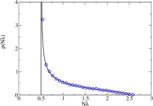
Figure 1: (Color online) Equilibrium density of the Coulomb fluid (Eq. (8)) when all the charges are constrained to the right of $\zeta=0.5$ (black solid line) together with the Monte Carlo simulations (blue circles) for the case $N=M=100$.

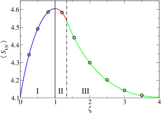
Figure 2: (Color online) Rate functions (top) and the average von Neumann entropy (bottom) as a function of the barrier position. Region I corresponds to $0\leq\zeta\leq 1$ when all the charges are on the right side of the barrier. Regions II and III corresponds to $1\leq\zeta\leq 4/3$ and $4/3\leq\zeta\leq 4$ respectively when all the charges are on the left side of the barrier. Monte Carlo simulations are shown in both the figures using black circles for $M=N=100$.

III.1 Evaluation of the density of states in Eq. (7) using the Coulomb gas method

The method of mapping the eigenvalues of a random matrix to a Coulomb gas problem goes back to Dyson Dyson621 ; Dyson622 ; Dyson623 ; Forresterbook . But a major development came when the Tricomi’s solution TricomiBook was used first in Satyalarge ; Satyalarge1 to compute the optimal charge densities and the associated rate functions of the extreme eigenvalues of the Gaussian ensembles. This ‘modified Coulomb gas’ has led to a lot of developments in the field of random matrix theory and its applications MajumdarNumber2012 ; Borot2012 ; SatyaMajumdar2011 ; Castillo2010 ; Pierpaolo2008 ; SatyaIndex2009 ; Marino2014 ; Damle2011 ; Grabsch2017 ; SNMajumdar2014 ; Texier2013 ; Satyalarge1 ; Grabsch2016 . For example, problems which include finding the distribution of the extreme eigenvalues of the Gaussian and Wishart matrices Satyalarge ; Satyalarge1 ; Vivo07 ; Satyalargeright ; Castillo2010 , quantum transport in chaotic cavities Pierpaolo2008 ; PierpaoloVivo2010 , the index distribution for the Gaussian random fields Alan2007 and the Gaussian ensemble SatyaIndex2009 ; SatyaMajumdar2011 . This method will be used extensively in this paper. The definition of the rate function will be given in the subsequent part of this subsection. The results obtained here will then be compared with the previously know in the last part of this subsection.

The unit trace constraint $\sum_{i=1}^{N}\lambda_{i}=1$ implies that the typical amplitude of the eigenvalues is $\lambda_{typ}\sim 1/N$. Whereas in the case of the Wishart ensemble $\lambda_{typ}^{W}\sim N$. This implies that the scaling with $N$, for large $N$, differs in both the cases. But it should be noted that the effect of the trace constraint does not imply the rescaling of the Wishart results by a factor of $1/N^{2}$. This effect of the trace constraint leads to a different and new behavior which includes a condensation transition, which is absent in the Wishart ensembles Nadal10 ; Nadal11 ; Borot2012 .

The density of states in Eq. (7) corresponds to the following probability:

$$\begin{split}P(N\lambda_{\mbox{min}}>\zeta)&=P(N\lambda_{1}>\zeta,N\lambda_{2}>\zeta,\ldots,N\lambda_{N}>\zeta)\\ &=\frac{\int_{\zeta}^{\infty}\ldots\int_{\zeta}^{\infty}P[\{\lambda_{i}\}]\prod_{i=1}^{N}d\lambda_{i}}{\int_{0}^{\infty}\ldots\int_{0}^{\infty}P[\{\lambda_{i}\}]\prod_{i=1}^{N}d\lambda_{i}},\end{split}$$ (9)

when all the eigenvalues are constrained to be larger than a fixed constant $\zeta$. The joint pdf of the eigenvalues $P[\{\lambda_{i}\}]$ given in Eq. (3) can be seen as a Boltzmann weight at inverse temperature $\beta$:

$$P[\{\lambda_{i}\}]\propto\exp\{-\beta E[\{\lambda_{i}\}]\},$$ (10)

where the energy $E[\{\lambda_{i}\}]=-\gamma\sum_{i=1}^{N}\ln\lambda_{i}-\sum_{i<j}\ln|\lambda_{i}-\lambda_{j}|$ and $\gamma=1/2-1/\beta$ (for $N=M$ case). This energy is the effective energy of a 2D Coulomb gas of charges where the charges repel each other electrostatically via logarithmic interaction in 2D. For large $N$, the presence of the logarithmic interaction potential term results in the effective energy to be of the order $E\sim O(N^{2})$. Thus, to compute the multiple integral in Eq. (9) the method of steepest descent is used. In this method, for large $N$, the configuration of $\{\lambda_{i}\}$ which dominates the integral is the one that minimizes the effective energy. For large $N$, it can be expected that the eigenvalues are close to each other. In that case the saddle point will be highly peaked, i.e. the most probable value and the mean will coincide. Thus, labeling the $\lambda_{i}$ by a continuous average density of states $\rho\left(\lambda,N\right)=N^{-1}\sum_{i}\langle\delta(\lambda-\lambda_{i})\rangle=N\,\rho(x)$ where

$$\rho(x)=N^{-1}\sum_{i}\langle\delta(x-\lambda_{i}N)\rangle$$ (11)

and $x=\lambda N$. Thus, the probability of $N\lambda_{\mbox{min}}$ greater than $\zeta$ can be written as

$$P(N\lambda_{\mbox{min}}>\zeta)\propto\int\mathcal{D}\left[\rho\right]\>\exp\left\{-\beta N^{2}\,E_{\zeta}\left[\rho\right]\right\}\,,$$ (12)

where the effective energy $E_{\zeta}\left[\rho\right]$ is given by

$$E_{\zeta}\left[\rho\right]=-\frac{1}{2}\int_{\zeta}^{\infty}\int_{\zeta}^{\infty}dx\,dx^{\prime}\>\rho(x)\rho(x^{\prime})\,\ln\left|x-x^{\prime}\right|$$

$$+\mu_{0}\left(\int_{\zeta}^{\infty}dx\>\rho(x)-1\right)+\mu_{1}\left(\int_{\zeta}^{\infty}dx\>x\>\rho(x)-1\right)\,.$$ (13)

The Lagrange multipliers $\mu_{0}$ and $\mu_{1}$ enforce the constraints $\int\rho(x)dx=1$ (the normalization of the density) and $\sum_{i}\lambda_{i}=1$ (the unit trace) respectively. For large $N$, the method of steepest descent gives the following:

$$P\left(N\lambda_{\mbox{min}}>\zeta\right)\propto\exp\left\{-\beta N^{2}E_{\zeta}\left[\rho_{\zeta}\right]\right\}\,,$$ (14)

where $\rho_{\zeta}$ minimizes the energy (the saddle point):

$$\frac{\delta E_{\zeta}}{\delta\rho}\Big{|}_{\rho=\rho_{\zeta}}=0\,.$$ (15)

This saddle point equation gives:

$$\int_{\zeta}^{\infty}dx^{\prime}\,\rho_{\zeta}(x^{\prime})\ln\left|x-x^{\prime}\right|=\mu_{0}+\mu_{1}x\,.$$ (16)

Differentiating with respect to $x$ gives:

$$\mathcal{P}\int_{\zeta}^{\infty}dx^{\prime}\,\frac{\rho_{\zeta}(x^{\prime})}{x-x^{\prime}}=\mu_{1}\,,$$ (17)

where $\mathcal{P}$ denotes the Cauchy principal value.

This singular integral equation can be solved by using the Tricomi’s theorem TricomiBook which states that if the solution $\rho^{*}$ has the finite support $[L_{1},L_{2}]$, then the finite Hilbert transform which is defined by the following equation

$$F(x)=\mathcal{P}\int_{L_{1}}^{L_{2}}dx^{\prime}\>\frac{\rho^{*}(x^{\prime})}{x-x^{\prime}}$$ (18)

can be inverted as

$$\begin{split}\rho^{*}(x)&=\frac{-1}{\pi^{2}\sqrt{x-L_{1}}\sqrt{L_{2}-x}}\bigg{[}C+\\ &\mathcal{P}\int_{L_{1}}^{L_{2}}dx^{\prime}\frac{\sqrt{x^{\prime}-L_{1}}\sqrt{L_{2}-x^{\prime}}}{x-x^{\prime}}\,F(x^{\prime})\bigg{]}\,,\end{split}$$ (19)

where $C=-\pi\int_{L_{1}}^{L_{2}}dx\,\rho^{*}(x)$. Here, $L_{1}=\zeta$ and $F(x)=\mu_{1}$. This solution was first used successfully in Ref.Satyalarge ; Satyalarge1 to study the large deviations of the extreme eigenvalues of Gaussian ensemble as mentioned in the beginning of this subsection.

The integral in Eq. (19) can be evaluated explicitly to obtain:

$$\begin{split}\rho^{*}(x)&=\frac{1}{\pi\sqrt{x-\zeta}\sqrt{L_{2}-x}}\\ &\bigg{[}1+\frac{(2\left(\zeta+L_{2})-4\right)(\zeta+L_{2}-2x)}{(\zeta-L_{2})^{2}}\bigg{]},\\ &\mbox{where}\;\;\zeta\leq x\leq L_{2}.\end{split}$$ (20)

Here, the normalization condition $\int_{\zeta}^{L_{2}}dx\,\rho^{*}(x)=1$ is used to set the constant $C=-\pi$. Whereas $\mu_{1}=4(\zeta+L_{2}-2)/(\zeta-L_{2})^{2}$ is obtained using the constraint $\int_{\zeta}^{L_{2}}dx\,x\,\rho^{*}(x)=1$. There is one more unknown $L_{2}$ which needs to be fixed. At the two end points $\zeta$ and $L_{2}$, the solution $\rho^{*}(x)$ either vanishes or has an inverse square root divergence (which is integrable). When there is no constraint the density has an inverse square root divergence at the origin and it vanishes at $4$. But when the minimum eigenvalue has to satisfy the constraint of being greater than $\zeta$ then intuitively it seems that the new density must have same nature at the boundary points as that of when there is no constraint. This is verified numerically for various values of $\zeta$ between zero and one. One such illustration is shown in Fig. 1. Thus, the condition $\rho(L_{2})=0$ gives $L_{2}=4-3\,\zeta$. Thus, the final density as a function of $\zeta$ is given as follows:

$$\rho(x)=\frac{1}{2\pi(1-\zeta)}\sqrt{\frac{4-3\zeta-x}{x-\zeta}},\;\;\zeta\leq x\leq 4-3\zeta.$$ (21)

Using $~{}L_{2}=4-3\zeta~{}$ the  constant $~{}\mu_{1}~{}$ simplifies to $1/(2(1-\zeta))$. The constant $\mu_{0}$ is found using Eq. (16) and  putting $~{}x=\zeta$. This gives $~{}\mu_{0}=\ln(1-\zeta)+(3\zeta-2)/(2(1-\zeta))$. Finally, the saddle point energy is calculated. First, the saddle point Eq. (16) is multiplied by $\rho(x)$ then the integration is carried out. Then using Eq. (III.1) one obtains

$$E_{\zeta}\left[\rho_{\zeta}\right]=3/4-\ln(1-\zeta)/2.$$ (22)

Now, the rate function for the large fluctuations will be calculated. It is defined as follows. For large $N$ the probability $P\left(N\lambda_{\mbox{min}}>\zeta\right)\approx\exp\{-\beta N^{2}\Phi(\zeta)\}$ where $\Phi(\zeta)$ is the rate function. The normalized probability is given as follows:

$$P\left(N\lambda_{\mbox{min}}>\zeta\right)\approx\frac{\int\mathcal{D}\left[\rho\right]\>\exp\left\{-\beta N^{2}\,E_{\zeta}\left[\rho\right]\right\}}{\int\mathcal{D}\left[\rho\right]\>\exp\left\{-\beta N^{2}\,E\left[\rho\right]\right\}}\,,$$ (23)

where $E_{\zeta}\left[\rho\right]$ is given in Eq. (22) and $E\left[\rho\right]$ is the effective energy associated to the joint distribution of the eigenvalues without any constraints obtained by putting $\zeta=0$ in the Eq. (22). Using the steepest descent method for both the numerator and the denominator one obtains the following:

$$\begin{split}P\left(N\lambda_{\mbox{min}}>\zeta\right)&\approx\frac{\exp\{-\beta N^{2}E_{\zeta}[\rho_{\zeta}]\}}{\exp\{-\beta N^{2}E[\rho^{*}]\}}\\ &\approx\exp\{-\beta N^{2}\Phi(\zeta)\},\end{split}$$ (24)

with $\Phi(\zeta)=E_{\zeta}\left[\rho_{\zeta}\right]-E\left[\rho^{*}\right]$ and where $\rho^{*}$ (resp. $\rho_{\zeta}$) is the density that minimizes the energy $E\left[\rho\right]$ (resp. $E_{\zeta}\left[\rho\right]$). The density $\rho^{*}(x)$ is thus simply the rescaled average density of states given in Eq. (4) (for $Q=1$) which corresponds to $\zeta=0$ case in Eq. (22). Finally, the rate function is given as follows:

$$\Phi(\zeta)_{I}=E_{\zeta}\left[\rho_{\zeta}\right]-E\left[\rho^{*}\right]_{\zeta=0}=-\frac{\ln(1-\zeta)}{2}\,$$ (25)

and is plotted in Fig. 2 (region I of top figure). It shows a divergence as $\zeta\rightarrow 1^{-}$. Whereas it vanishes at $\zeta=0$ which is consistent with the no constraint condition. The theoretically obtained curve is compared the numerically obtained rate function using the Monte Carlo simulations and both of them agrees very well with each other. The large deviations for the minimum eigenvalue of the Wishart ensemble (where there is no trace constraint) is studied earlier in Ref.Castillo2010 . Our results, namely the rate function in the Eq. (25) and the density of states of the Coulomb charges differ from that of Ref.Castillo2010 . These differences can be attributed to the trace constraint on the reduced density matrices.

Now, the connection of our results to the previously known ones is given. The full distribution, for all $N=M$, of the minimum Schmidt eigenvalue and the minimum eigenvalue of Wishart ensemble is known RMTBook . An exact relation between the two is also known RMTBook . These results have been evaluated for the three cases of $\beta=1$, $2$ and $4$. From these earlier results it can be seen easily that the large deviation tail is $(1-\zeta)^{(\beta N^{2}/2)}$ which gives the rate function as $-(1/2)\ln(1-\zeta)$. This expression agrees with our expression for $\Phi(\zeta)_{I}$. But our calculations, using the Coulomb gas method from Satyalarge ; Satyalarge1 , shows that this expression for the rate function holds for all the values of $\beta$ and not just for these three values. The connections of the rate function $\Phi(\zeta)_{I}$ and the corresponding equilibrium density in Eq. (21) to those of maximum eigenvalue will be given in the next section.

IV Review of results of the maximum eigenvalue

In this section, a short review on the relevant results of the maximum eigenvalue will be given. These results will be used in the subsequent parts of this paper. The question addressing the constraint on all the eigenvalues being less than a fixed constant $\zeta$ is studied in detail earlier in Nadal11 using the modified Coulomb gas method from Ref.Satyalarge ; Satyalarge1 . This constraint is equivalent to the condition that $\lambda_{\mbox{max}}\leq\zeta$. For equal dimensionality $N=M$ case i.e. $Q=1$ the rescaled eigenvalues lie in the interval $(0,4]$ (refer Eq. (4)). Thus, the barrier position $\zeta$ is effective only when $\zeta\leq 4$. Since, $\lambda_{\mbox{max}}$ satisfies the condition $1/N\leq\lambda{\mbox{max}}\leq 1$ which implies $1\leq\zeta\leq 4$. Throughout this paper, whenever $\zeta$ lies between zero (one) and one (four) it refers to the fact $N\lambda_{\mbox{min}}\geq\zeta$ ($N\lambda_{\mbox{max}}\leq\zeta$).

In Ref.Nadal11 it was shown that there are two regions depending on the nature of the density which shows a transition at $\zeta=4/3$. Thus, there are two sub cases. Case one ($4/3\leq\zeta\leq 4$): the density has a support on $[0,\zeta]$ and has a divergence at both the boundaries except at $\zeta=4/3$ where the density vanishes at the origin. Case two ($1\leq\zeta\leq 4/3$): the density has a support on $[4-3\zeta,\zeta]$. In this case it vanishes at $4-3\zeta$ and has a divergence at $\zeta$. The density in the first case is given as

$$\rho(x)=\frac{2\zeta^{2}+4(\zeta-2)(\zeta-2x)}{2\pi\zeta^{2}\sqrt{x(\zeta-x)}},\;\;0\leq x\leq\zeta;$$ (26)

whereas in the second case it is given as

$$\rho(x)=\frac{1}{2\pi(\zeta-1)}\sqrt{\frac{3\zeta-4+x}{\zeta-x}},\;\;4-3\zeta\leq x\leq\zeta.\\$$ (27)

The rate functions were also derived in Nadal11 . For the first case it is given as

$$\Phi(\zeta)_{III}=\dfrac{3}{4}-4\dfrac{\zeta-1}{\zeta^{2}}-\dfrac{1}{2}\ln\left(\dfrac{\zeta}{4}\right)$$ (28)

and is plotted in Fig. 2 (region III of the top figure). It vanishes at $\zeta=4$ which is consistent with the no constraint condition. Whereas for the second case it is given as

$$\Phi(\zeta)_{II}=-\dfrac{\ln(\zeta-1)}{2}$$ (29)

and is plotted in Fig. 2 (region II of top figure). It can be seen from Eq. (25) that the rate functions $\Phi(\zeta)_{I}$ (derived in Sec. III of this paper) and $\Phi(\zeta)_{II}$ are reflections of each other around $\zeta=1$, in fact it can be seen from the densities in Eqs. (27) and (7) that both are reflections of each other around $\zeta=1$ provided $2/3\leq\zeta\leq 1$ is used for the deviations of the minimum eigenvalue.

The large deviations for the maximum eigenvalue of the Wishart ensemble (where there is no trace constraint) is studied in Ref.Vivo07 . But, no transition in the density as well as the rate function is observed there, which can be attributed to the absence of the trace constraint on the matrices. For the $N=M$ case in Ref.Vivo07 the density shows divergence at both the ends of its eigenvalue support whenever $\lambda_{\mbox{max}}<4$.

V Bipartite entanglement

In the earlier works in Ref.Nadal10 ; Nadal11 , using the Coulomb gas method the full probability distribution of the Renyi entropy, a measure of bipartite entanglement of which von Neumann entropy is a special case, is derived. There, two critical points are found for which the charge density shows a transition as the value of Renyi entropy is varied. In the first transition, the integrable singularity at the origin disappears while in the second, the largest eigenvalue gets detached from the continuum sea of all the other eigenvalues. As explained in Sec.IV the density shows a transition when there are large deviations in the maximum eigenvalue while no such transition is observed for the same in the minimum eigenvalue.

In the introduction of this paper importance of the extreme eigenvalues from the perspective of entanglement between subsystems $A$ and $B$ is given. But, what is the actual entanglement measured using the von Neumann entropy for given constraints (case of large deviations here) on these extreme eigenvalues is unanswered. Thus, in this section our aim is to quantify the bipartite entanglement between subsystems $A$ and $B$ when there are large deviations in the extreme eigenvalues from their average values. We would also like to investigate that does the signature of presence or absence of transition in the densities are reflected in the entropies or not. Here, the von Neumann entropy is used as a measure of entanglement Bennett96 ; Zyczkowski06 . For this study the optimal Coulomb charge densities obtained in Sec.III and the ones from earlier studies reviewed in Sec.IV will be used. It should be noted that when there no large deviations in the extreme eigenvalues the average von Neumann entropy is known as Page’s formula Page and is given in Eq.(6). Thus, with this conditional average generalization of this formula will also be addressed. Results obtained in this section and those on tripartite entanglement in the next section are compared qualitatively from the perspective of monogamous nature of entanglement at the end of next section.

As a first case, the large deviations in the case of maximum eigenvalue is considered. As pointed out in the earlier parts of this paper, there are two sub cases depending on the position of the barrier. Using Eq. (2) and labeling the eigenvalues of $\rho_{A}$ by a continuous average density of states as done in Sec. III.1 the average von Neumann entropy is given as

$$\langle S_{VN}\rangle=-N\int x\ln(x)\rho(x)dx$$ (30)

where the form of $\rho(x)$ is given in Eq. (11). One needs to use the appropriate expression of the charge density $\rho(x)$ depending on the value of $\zeta$ for calculating the average entropy. For the case when $4/3\leq\zeta\leq 4$ the density given in the Eq. (26) is used in Eq. (30) to calculate the average entropy. Then using Mathematica 9 it is found to be

$$\ln\left(\frac{4N}{\zeta}\right)+\frac{\zeta}{4}-\frac{3}{2}.$$ (31)

It is plotted in Fig. 2 for the case $N=100$ (region III of the bottom figure). For the special case of $\zeta=4$ which corresponds to no constraint on the maximum eigenvalue, the average von Neumann entropy turns out to be $\ln(N)-1/2$ Page . This value agrees very well with that derived in Ref.Page where there are no additional constraints on the eigenvalues of $\rho_{A}$.

For the second case when $1\leq\zeta\leq 4/3$ the density given in the Eq. (27) is used in Eq. (30) to obtain the average von Neumann entropy. Again using Mathematica 9 it turns as follows:

$$\ln(N)-\frac{1}{\zeta(4-3\zeta)}\bigg{(}(\zeta-a)^{2}(3\zeta-4)\times$$

$${}_{p}F_{q}\left[\{1,1,3/2\},\{3,4\},\frac{4(\zeta-1)}{3\zeta-4}\right]+$$

$$2(\zeta-1)^{2}(9\zeta-10)_{p}F_{q}\left[\{1,1,5/2\},\{3,4\},\frac{4(\zeta-1)}{3\zeta-4}\right]$$

$$-(3\zeta-4)\left(8-19\zeta+11\zeta^{2}+\zeta\ln\left(4-3\zeta\right)\right)\bigg{)}$$ (32)

where ${}_{p}F_{q}\left[a,b,z\right]$ is the generalized hypergeometric function. It is plotted in Fig. 2 for $N=100$ (region II of the bottom figure). The special case when $\zeta=1$ is now considered. In that case the maximum eigenvalue is equal to $1/N$ which implies the von Neumann entropy is $\ln(N)$ which is also the maximum value it can take as explained in the introduction of the paper. It can also be evaluated using the Eq. (V). The entropy for $N=100$ indeed equals $\ln(100)\approx 4.605$. The Eqs. (31) and (V) are compared with the Monte Carlo simulations as shown in bottom figure of Fig. 2. It can be seen that the numerical simulations agrees very well with the analytical results.

At $\zeta=4/3$ (the transition between regimes II and III), the average von Neumann entropy $\langle S_{VN}\rangle$ has a nonanalyticity. It is continuous with $\langle S_{VN}\rangle(4/3)=\ln(3N)-7/6$ and once differentiable with $\frac{d\langle S_{VN}\rangle}{d\zeta}\big{|}_{\zeta=4/3}=-1$. However, the second derivative is discontinuous: $\frac{d^{2}\langle S_{VN}\rangle}{d\zeta^{2}}\big{|}_{\zeta=4/3^{-}}=-9/2$ but $\frac{d^{2}\langle S_{VN}\rangle}{d\zeta^{2}}\big{|}_{\zeta=4/3^{+}}=9/16$. Thus, similar to rate function the von Neumann entropy shows a discontinuity but in its second derivative at $\zeta=4/3$. Thus, the signature of the transition in the density of states can be observed in the von Neumann entropy.

Now, the case of the large deviations of the minimum eigenvalue is considered. The barrier position $\zeta$ satisfies $0\leq\zeta\leq 1$. Computing analytical expression for the entropy is difficult. Thus, it is evaluated numerically using the density in Eq. (21) and Eq. (30) for the case of $N=100$. It is plotted in Fig. 2 (region I of the bottom figure) along with the Monte Carlo simulations. It can be seen that both agree with each other very well. It can be seen easily from the figure the entropy is continuous and infinitely differentiable in the region I since it is concave downward. This can be attributed to the fact that density don’t show any transition in this case.

VI Entanglement within subsystems

In this section, the subsystem $A$ is further divided into two parts denoted as $1$ and $2$ having Hilbert space dimension $N_{1}$ and $N_{2}$ respectively such that $N=N_{1}N_{2}$. Then the effect of the large deviations of the extreme eigenvalues of $\rho_{A}$ are studied on the entanglement between the subsystems $1$ and $2$. Now, we have a tripartite pure state having dimensions $N_{1}$, $N_{2}$ and $M$. The entanglement in such a tripartite pure system when its state is chosen randomly, has been studied previously in Ref.Uday12 ; Aubrun12 ; Aubrun2014 . There it is shown that the entanglement between subsystems $1$ and $2$ shows a transition at $M=4N_{1}N_{2}$ for sufficiently large subsystem dimensions.

The entanglement between subsystems $1$ and $2$ is studied using the log negativity measure vidal . It is defined as $E_{LN}(\rho_{12})=\log(||\rho_{12}^{\Gamma}||)$, where $||\rho^{\Gamma}||$ is the trace norm of the partial transpose (PT) matrix $\rho^{\Gamma}$ peres96 . When the log negativity is greater than zero, the state is said to have the negative partial transpose (NPT). Then the state is entangled. When the log negativity is zero, the state is said to have the positive partial transpose (PPT). Then the state is either separable or bound entangled mhorodeckibound .

Now, the numerical procedure to generate random states $\rho_{12}$ having large deviations in their extreme eigenvalues is given. Every density matrix, which is Hermitian, can be diagonalized by an unitary rotation $U$. It is thus natural that the distribution of eigenvalues and that of eigenvectors of $\rho_{12}$ are independent. Thus, the probability measure of $\rho_{12}$ factorizes in a product form Sommers ; Hall1998 , $\mbox{d}\mu_{x}=\mbox{d}\nu_{x}(\lambda_{1},\lambda_{2},\ldots,\lambda_{N})\times\mbox{d}h$. Here, $\lambda_{1},\lambda_{2},\ldots,\lambda_{N}$ are the eigenvalues of $\rho_{12}$ and the factor $\mbox{d}h$ determines the distribution of its eigenvectors. The probability measure used for the eigenvalues is given in Eq. (3) along with the constraint on the extreme eigenvalues. For the measure $\mbox{d}h$ the unique Haar measure on $U(N)$ is taken which determines the statistical properties of the eigenvectors forming $U$. Thus, this gives $\rho_{12}=Ud\,U^{\dagger}$ where $d$ is a diagonal matrix $[\lambda_{1},\lambda_{2},\ldots,\lambda_{N}]$. The eigenvalues are generated numerically using the Monte Carlo method. Whereas the matrix $U$ is generated using the algorithm given in Ref.Mezzadri2007 .

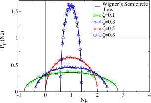
Figure 3: (Color online) Density of states of $\rho_{12}^{\Gamma}$ for various values of barrier positions $\zeta$ between zero and one. All the eigenvalues of randomly chosen $\rho_{12}$ are greater than the barrier position. One thousand such matrices are used for each $\zeta$. It corresponds to the large deviations of the minimum eigenvalue $(0\leq\zeta\leq 1)$. A vertical line at the origin has been shown to draw attention to the negative part of the spectrum. Here, $N_{1}=N_{2}=10$ and $M=100$.

Earlier works have studied the effect of PT on $\rho_{12}$ in tripartite random pure states Uday12 ; Aubrun12 ; Aubrun2014 . It is shown that the density of $\rho_{12}$ after PT is very close to the Wigner’s semicircle law when the dimensions of both the subsystems are not too small and are of the same order. In fact, the Wigner’s semicircle law is also obtained in a bipartite mixed state $\rho_{12}$ after PT which is obtained by uniformly mixing sufficiently large number of random bipartite pure states Marko . But in this paper our focus is on the bipartite and tripartite random pure system. In these works the extreme eigenvalues fluctuates around their average values. In Ref.Uday12 the minimum eigenvalue of $\rho_{12}^{\Gamma}$ is shown to follow the Tracy-Widom distribution. Using this the fraction of entangled states at criticality ($M=4N_{1}N_{2}$) was given. This suggests to investigate the effects of the large deviations of the extreme eigenvalues of $\rho_{12}$ on the density of $\rho_{12}^{\Gamma}$ as well as on the entanglement between subsystems $1$ and $2$. The results are plotted in Figs. 3, 4 and 5 for the case $N_{1}=N_{2}=10$ and $M=100$. It can be seen that the eigenvalue densities of $\rho_{12}^{\Gamma}$ is very close to the Wigner semicircle law. As the barrier position is changed an entanglement transition takes place from dominantly NPT states to dominantly PPT.

It should be mentioned here that the case $N_{1}\neq N_{2}$ without any large deviations in the extreme eigenvalues has been studied in Uday12 . There it was shown that the density of states of $\rho_{12}^{\Gamma}$ had a skewness which was calculated analytically. It is also observed in our work that the density has a skewness (not presented here) but calculating it analytically seems to be mathematically challenging. Thus, it is not addressed in this paper.

VI.1 Model for shifted semicircles

In the earlier work in Ref.Uday12 the semicircular density of $\rho_{12}^{\Gamma}$ was well studied using a simple model. It was suggested by using the fact that the first two moments remains unchanged under the PT operation. The semicircular density depends only on two moments, the mean and the variance. Thus, it was proposed to shift and scale the semicircle of the Gaussian ensembles such that the first two moments of $\rho_{12}$ are matched. To explain the semicircular density obtained in this paper the same model from Ref.Uday12 is used. The model has been used to accurately predict the transition from the dominantly NPT states to the dominantly PPT states.

Now, the model for the shifted semicircles is given. Here, it is assumed that these random matrices are sampled from the Gaussian unitary ensemble (GUE). Thus, consider

$$Y=X+\dfrac{I_{N}}{N}$$ (33)

where $X$ is a $N\times N$ random matrix from the GUE ensemble with the necessary matrix element variance such that it matches with that of $\rho_{12}$, and $I_{N}$ is the identity matrix of dimension $N$. It can be seen that $\langle\mbox{tr}(Y)\rangle=1$ since $\langle\mbox{tr}(X)\rangle=0$, where the angular brackets indicates the ensemble average. Here, the case of large matrix dimension is considered. Thus, it can be expected that the influence of the fact that the $\mbox{tr}(Y)$ is not exactly equal to one for each and every member of the ensemble will not be observed except in the case of very small dimensional cases.

It can be seen that the eigenvalues of $Y$ are all those of $X$ shifted by $1/N$. Thus, considering the spectrum of $X$ alone will be sufficient. Under the assumption that $X$ is sampled from the GUE it follows that the density of eigenvalues of $Y$ for large $N$ is given as follows:

$$P(\mu)=\frac{2}{\pi R^{2}}\sqrt{R^{2}-\bigg{(}\mu-\frac{1}{N}\bigg{)}^{2}},\;-R+\frac{1}{N}<\mu<R+\frac{1}{N},$$ (34)

where

$$R=2\sqrt{\dfrac{1}{N}\langle\mbox{tr}(X^{2})\rangle}=2\sqrt{\frac{1}{N}\langle\mbox{tr}(\rho_{12}^{2})\rangle\,-\,\frac{1}{N^{2}}}.$$ (35)

Now, the scaled variable $x=\mu N$ is used. This results into the semicircular probability density having a shift of $1$ and a rescaled “radius” $\tilde{R}=NR$. Explicitly:

$$P_{\Gamma}(x)=\frac{2}{\pi\tilde{R}^{2}}\sqrt{\tilde{R}^{2}-(x-1)^{2}},\;\;1-\tilde{R}<x<1+\tilde{R}.$$ (36)

This is the the Wigner semicircle law that has been observed in Figs. (3) and (4). Now, $\tilde{R}$ is calculated when there are large deviations in the extreme eigenvalues. This requires to find the average purity of $\rho_{12}$. First, the case of large deviations of the minimum eigenvalue is considered. Using the density of states in Eq. (7) in Mathematica 9, the purity turns out to be $\langle\mbox{tr}(\rho_{12}^{2})\rangle=P_{1}/N=(2-2\zeta+\zeta^{2})/N$. This gives the rescaled radius $\tilde{R}=2(1-\zeta)$ where $0\leq\zeta\leq 1$. Similarly, for the case of the large deviations of the maximum eigenvalue, the density of states in Eqs. (27) and (26) is used. The purity is found to be $P_{2}/N=(2-2\zeta+\zeta^{2})/N$ and $P_{3}/N=-\zeta(\zeta-8)/(8N)$ for $1\leq\zeta\leq 4/3$ and $4/3\leq\zeta\leq 4$ respectively. Here, $P_{1}$, $P_{2}$ and $P_{3}$ are the rescaled purities. Using these purities $\tilde{R}$ equals $2(\zeta-1)$ and $2\sqrt{(-\zeta^{2}+8\zeta-8)/8}$ for $1\leq\zeta\leq 4/3$ and $4/3\leq\zeta\leq 4$ respectively. It can be seen that these analytical expressions for the rescaled radii agrees very well with those from Figs. (3) and (4).

This model gives the NPT-PPT transition very well. It can be seen that the condition for this transition is $\tilde{R}=1$. Using this condition one obtains $\zeta=1/2$ and $4-\sqrt{6}$ as the transition points for the large deviations of the minimum and maximum eigenvalue respectively. For any $\zeta>1/2$ in the case of minimum eigenvalue and $\zeta<4-\sqrt{6}$ in the case of maximum eigenvalue the radius is smaller than one and there are predominantly PPT states. Whereas in the opposite cases the lower bounds are such that there are predominantly NPT states. Thus, this simple model from Ref.Uday12 of a shifted random matrix of the GUE kind for the partial transpose gives the transition very well. These critical values of the barrier positions can be observed in Figs. (3) and (4).

In Ref.Uday12 it was shown analytically that before and after the PT the range of the eigenvalues is the same. Extreme deviations from this result were shown to occur when the state $\rho_{12}$ is pure or nearly pure. For the large deviation of the minimum eigenvalue the density before PT has a support on $[\zeta,4-3\zeta]$ and after PT it becomes $[1-\tilde{R},1+\tilde{R}]$ where $\tilde{R}=2(1-\zeta)$ where $0\leq\zeta\leq 1$. Thus, the range of the eigenvalues before and after the PT are both equal to $4(1-\zeta)$.

Similarly, for the large deviations of the maximum eigenvalue the density before PT has a support on $[4-3\zeta,\zeta]$ and $[0,\zeta]$ for $1\leq\zeta\leq 4/3$ and $4/3\leq\zeta\leq 4$ respectively. After PT the support is again $[1-\tilde{R},1+\tilde{R}]$ but with $\tilde{R}=2(\zeta-1)$ and $2\sqrt{(-\zeta^{2}+8\zeta-8)/8}$ for $1\leq\zeta\leq 4/3$ and $4/3\leq\zeta\leq 4$ respectively. Thus, it can be seen that only for $1\leq\zeta\leq 4/3$ the range of the eigenvalues before and after PT equals $4(\zeta-1)$. This range is reflection symmetry of that corresponding to the large deviations of the minimum eigenvalue around $\zeta=1$. While for $4/3\leq\zeta\leq 4$ the range of the eigenvalues after PT is larger than that of before PT except at $\zeta=4/3$ and $4$ where both the ranges are equal. It should be mentioned that these results are valid for the case $N_{1}\neq N_{2}$ since they depend only on $N=N_{1}N_{2}$ and $M$. But when $N_{1}$ and $N_{2}$ differ significantly the density of states of $\rho_{12}^{\Gamma}$ has a skewness whereas the model predicts zero skewness.

VI.2 Logarithmic negativity

The average log negativity between two subsystems 1 and 2 is now studied. The formalism from Ref.Uday12 is used again where the fact that the density of states after PT is Wigner’s semicircle was used. There it is shown analytically that

$$\langle E_{LN}\rangle_{M}=\log\Bigg{[}\frac{2}{\pi}\sin^{-1}\Big{(}\frac{1}{\tilde{R}}\Big{)}+\frac{2}{3\pi\tilde{R}}\sqrt{1-\frac{1}{\tilde{R}^{2}}}\left(1+2\tilde{R}^{2}\right)\Bigg{]}.$$ (37)

Here, $\langle E_{LN}\rangle_{M}$ denotes the log negativity obtained using the simple model. This formula is valid only for $\tilde{R}\geq 1$ otherwise $\langle E_{LN}\rangle_{M}$ is zero. For our case, $\tilde{R}=NR=2(1-\zeta)$ $(0\leq\zeta\leq 1)$ for the large deviations of the minimum eigenvalue. Whereas, $\tilde{R}$ is $2(\zeta-1)$ and $2\sqrt{(-\zeta^{2}+8\zeta-8)/8}$ for $1\leq\zeta\leq 4/3$ and $4/3\leq\zeta\leq 4$ respectively for the large deviations of the maximum eigenvalue. For the critical case $\tilde{R}=1$ this formula gives zero for the average log negativity. When $\tilde{R}<1$, the states obtained are predominantly PPT. In that case $\langle E_{LN}\rangle=0$. Thus, it can be seen that $\langle E_{LN}\rangle=0$ for $1/2\leq\zeta\leq 4-\sqrt{6}$ since $\tilde{R}\leq 1$ for this range of $\zeta$ as shown in the previous subsection. The Eq. (37) is plotted in Fig. 5 along with numerical results for various values of $\zeta$ for $N_{1}=N_{2}=10$ and $M=100$. It can be seen that Eq. (37) works very well. Consider the situations in which there are no constraints on either of the extreme eigenvalues. It implies $\zeta=0$ ($\zeta=4$) for the minimum (maximum) eigenvalue. This gives $\tilde{R}=2$ for both of them. In that case the Eq. (37) gives $\langle E_{LN}\rangle\approx 0.148702$. This value can be observed in Fig. 5 at $\zeta=0$ and $\zeta=4$.

Another interesting features that is observed in Fig. 5 is that there are two different values of $\zeta$’s ($\zeta_{1}$ and $\zeta_{2}$, say) corresponding to the large deviations of the extremes for which entanglement between subsystems $1$ and $2$ is same. Here, $\zeta_{1}$ ($\zeta_{2}$) corresponds to the large deviation of the minimum (maximum) eigenvalue. Thus, this implies $0\leq\zeta_{1}\leq 1$ and $1\leq\zeta_{2}\leq 4$. It can be seen that from Eq. (37) for the log negativity, derived using the simple random matrix model, that two different $\zeta$’s will result in the same log negativity provided $\tilde{R}$ is same for both of them. Whereas in Eq. (35) it is shown that $\tilde{R}$ depends only on the purity of $\rho_{12}$. Thus, this implies that large deviations of the extremes will have the same log negativity if the corresponding purities (so does the rescaled purities) are same.

Using the simple model it is shown that log negativity is non-zero when $\zeta<1/2$ ($\zeta>4-\sqrt{6}$) for the large deviation of the minimum (maximum) eigenvalue. Thus, it is sufficient to consider the rescaled purities $P_{1}$ and $P_{3}$ to find the desired relation between $\zeta_{1}$ and $\zeta_{2}$. For given $\zeta_{1}$ the rescaled purity is $P_{1}=2-2\zeta_{1}+\zeta_{1}^{2}$. The parameter $\zeta_{2}$ for which the rescaled purity is $P_{1}$ one needs to solve for $P_{1}=P_{3}=(8\zeta_{2}-\zeta_{2}^{2})/8$. Solving this quadratic equation one obtains $\zeta_{2}=4\pm 2\sqrt{2(2-P_{1})}=4\pm 2\sqrt{2\zeta_{1}-\zeta_{1}^{2}}$. Of these two solutions only $\zeta_{2}=4-2\sqrt{2(2\zeta_{1}-\zeta_{1}^{2})}$ is valid while the other solution is invalid since it exceeds its upper limit which is four. For the special value of $\zeta_{1}=1/8$ the corresponding value of $\zeta_{2}$ for which the log negativity is same is approximately equal to $2.6307$. Using Eq. (37) the log negativity is approximately equal to $0.0919$. These results can be observed in Fig. 5. It should be mentioned that these results are valid for the case $N_{1}\neq N_{2}$ since they depend only on $N=N_{1}N_{2}$ and $M$.

It is important to compare the results obtained in Secs.V and VI using the Fig. (5) and the bottom one in Fig. (2). In can be seen that at $\zeta=1$ the von Neumann entropy is maximum while the log negativity is zero. As $\zeta$ goes away from $1$ the von Neumann entropy reduces while the log negativity increases outside the range $[1/2,4-\sqrt{6}]$. This behavior can be understood using the monogamous nature of the entanglement Coffman . It says that if two subsystems (here subsystems $1$ and $2$) have maximum quantum corrections then they (either $1$ or $2$) cannot be correlated at all with a third system (here subsystem $B$). This also implies that the joint system of $1$ and $2$ together also cannot be correlated at all with the third system. Monogamy of entanglement holds for each and every quantum state which implies it will also hold on an average. This is what is observed from these figures. It should be noted that this is a qualitative observation and a quantitative understanding demands thorough investigation.

Figure 4: (Color online) Density of states of $\rho_{12}^{\Gamma}$ for various values of barrier positions $\zeta$ between one and four. All the eigenvalues of randomly chosen $\rho_{12}$ are smaller than the barrier position. One thousand such matrices are used for each $\zeta$. It corresponds to the large deviations of the maximum eigenvalue $(1\leq\zeta\leq 4)$. A vertical line at the origin has been shown to draw attention to the negative part of the spectrum. Here, $N_{1}=N_{2}=10$ and $M=100$.

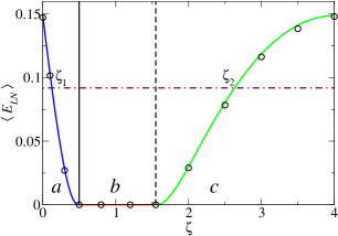
Figure 5: (Color online) Average entanglement in random states $\rho_{12}$ as measured by the log negativity between subsystems $1$ and $2$ for various barrier positions. This is compared with the analytical result in Eq. (37) based on the simple model. Black solid vertical line (dotted line) corresponds to $\zeta=1/2$ ($\zeta=4-\sqrt{6}$) showing the entanglement transition due to large deviations of the minimum (maximum) eigenvalue. Horizontal dash-dotted line is drawn such that $\zeta$ between $0$ and $1$ corresponding to its intersection with the log negativity is $1/8$. Regions $a$, $b$ and $c$ corresponds to $0\leq\zeta\leq 1/2$, $1/2\leq\zeta\leq 4-\sqrt{6}$ and $4-\sqrt{6}\leq\zeta\leq 4$ respectively. Here, $N_{1}=N_{2}=10$ and $M=100$.

VII SUMMARY AND CONCLUSIONS

This paper has studied the large deviations of the minimum Schmidt eigenvalue in a large bipartite system, denoted as $A$ and $B$. The state of the system is pure and chosen randomly from the uniform Haar measure. This eigenvalue play an important role in the study of entanglement between the two subsystems. Using the Coulomb gas method, the large deviation function for the minimum eigenvalue and the associated equilibrium charge density is derived. Our results hold for all the values of the Dyson index. These analytical expressions are found to agree very well with the Monte Carlo simulations. Thus, with this density the generalization of the Marcenko-Pastur function is given when there are large deviations in the minimum Schmidt eigenvalue. In this paper the case of equal dimensions ($N=M$) of subsystems $A$ and $B$ is studied.

The effect of the large deviations of both maximum and minimum eigenvalue is studied on the entanglement between $A$ and $B$ by using the von Neumann entropy. For this the equilibrium Coulomb charge density obtained for the large deviations of the minimum eigenvalue in this paper and the corresponding result for the maximum eigenvalue from earlier work in Ref.Nadal11 is used. In the case of large deviations of the maximum eigenvalue analytical expression for the entropy is derived using Mathematica 9, while the same for the minimum eigenvalue remains an open question. The entropy in the later case is obtained by numerical integration. These entropies are found to agree very well with the Monte Carlo simulations. The entropy corresponding to the large deviations of the maximum eigenvalue is continuous and once differentiable, but the second derivative is discontinuous at $\zeta=4/3$. This is due to the transition in the density of states occurring at same $\zeta$ because of the large deviations in the maximum eigenvalue Nadal11 .

One of the subsystem is further divided into two parts, denoted as $1$ and $2$. The effect of the large deviations is also studied on the entanglement, measured using the log negativity, between $1$ and $2$. It is found that the state of the subsystem undergoes a NPT-PPT transition. The transition takes place at $\zeta=0.5$ ($\zeta=4-\sqrt{6}$) for the large deviations of the minimum (maximum) eigenvalue. To be precise, when $\zeta>1/2$ ($\zeta<4-\sqrt{6}$) for the large deviations of the minimum (maximum) eigenvalue the states are dominantly PPT, the critical barrier position being $\zeta=1/2$ ($\zeta=4-\sqrt{6}$).

It is found numerically that the density of states of the reduced density matrix of subsystems after PT is close to the Wigner semicircle law when there are large deviations in the extreme Schmidt eigenvalues. The skewness of the semicircle is minimum for the symmetric case $N_{1}=N_{2}$. Earlier work in Ref.Uday12 has shown the same when there are no such large deviations. Thus, our work shows the robustness of the Wigner semicircle law after PT even in the presence of large deviations in the extreme eigenvalues before PT. A simple random matrix model from the same work in Ref.Uday12 is used successfully to capture the NPT-PPT transition as well as the density of states after PT. One to one relationship between barrier positions $\zeta_{1}$ and $\zeta_{2}$, which corresponds to large deviations of minimum and maximum eigenvalues respectively, is found such that the entanglement between subsystems $1$ and $2$ is same for both the positions. Results of bipartite and tripartite entanglement are interpreted qualitatively from the perspective of monogamous nature of the entanglement.

VIII Acknowledgments

Author is very grateful to acknowledge many discussions with Arul Lakshminarayan and Karol Życzkowski. Author is happy to acknowledge many discussions with M. S. Santhanam and T. S. Mahesh. The author thanks C. S. Sudheer Kumar, G. Khairnar, H. Tekur, and S. Paul for carefully reading the manuscript. The author acknowledges the funding received from Department of Science and Technology, India under the scheme Science and Engineering Research Board (SERB) National Post Doctoral Fellowship (NPDF) file Number PDF/2015/00050.

References

- (1) F. D. Hollander, Large Deviations (American Mathematical Society, 2000)
- (2) P. Vivo, S. N. Majumdar, and O. Bohigas, J. Phys. A: Math. Theor. 40, 4317 (2007)
- (3) D. S. Dean and S. N. Majumdar, Phys. Rev. Lett. 97, 160201 (2006)
- (4) D. S. Dean and S. N. Majumdar, Phys. Rev. E 77, 041108 (2008)
- (5) F. L. Metz and I. Pérez Castillo, Phys. Rev. Lett. 117, 104101 (2016)
- (6) E. Katzav and I. Pérez Castillo, Phys. Rev. E 82, 040104 (2010)
- (7) S. N. Majumdar, C. Nadal, A. Scardicchio, and P. Vivo, Phys. Rev. Lett. 103, 220603 (2009)
- (8) C. Nadal, S. N. Majumdar, and M. Vergassola, Phys. Rev. Lett. 104, 110501 (2010)
- (9) A. Lakshminarayan, S. Tomsovic, O. Bohigas, and S. N. Majumdar, Phys. Rev. Lett. 100, 044103 (2008)
- (10) S. N. Majumdar, O. Bohigas, and A. Lakshminarayan, J. Stat. Phys. 131, 33 (2008)
- (11) C. Nadal, S. N. Majumdar, and M. Vergassola, J. Stat. Phys. 142, 403 (2011)
- (12) U. T. Bhosale, S. Tomsovic, and A. Lakshminarayan, Phys. Rev. A 85, 062331 (2012)
- (13) K. Szymański, B. Collins, T. Szarek, and K. Życzkowski, Journal of Physics A: Mathematical and Theoretical 50, 255206 (2017)
- (14) P. Vivo, J. Phys. A: Math. Theor., P01022(2011)
- (15) M. Chavez, M. Ghil, and J. Urrutia-Fucugauchi, Extreme Events: Observations, Modeling, and Economics (Wiley, 2015)
- (16) S. Albeverio, V. Jentsch, and H. Kantz, Extreme Events in Nature and Society (Springer-Verlag Berlin Heidelberg, 2006)
- (17) S. S. Wilks, Mathematical Statistics (Princeton University Press, New Jersey, 1947)
- (18) K. Fukunaga, Introduction to Statistical Pattern Recognition (Elsevier, New York, 1990)
- (19) M. Fridman, R. Pugatch, M. Nixon, A. A. Friesem, and N. Davidson, Phys. Rev. E 85, 020101 (2012)
- (20) J. G. Richens, J. H. Selby, and S. W. Al-Safi, Phys. Rev. Lett. 119, 080503 (2017)
- (21) R. Horodecki, P. Horodecki, M. Horodecki, and K. Horodecki, Rev. Mod. Phys. 81, 865 (2009)
- (22) C. H. Bennett, G. Brassard, C. Crépeau, R. Jozsa, A. Peres, and W. K. Wootters, Phys. Rev. Lett. 70, 1895 (1993)
- (23) C. H. Bennett and S. J. Wiesner, Phys. Rev. Lett. 69, 2881 (1992)
- (24) C. H. Bennett, H. J. Bernstein, S. Popescu, and B. Schumacher, Phys. Rev. A 53, 2046 (1996)
- (25) I. Bengtsson and K. Zyczkowski, Geometry of Quantum States: An Introduction to Quantum Entanglement (Cambridge University Press, Cambridge, 2006)
- (26) J. W. Demmel, Math. Comput. 50, 449 (1988)
- (27) A. Edelman, Math. Comput. 58, 185 (1992)
- (28) M. Znidaric, J. Phys. A: Math. Theor. 40, F105 (2007)
- (29) Y. Chen, D.-Z. Liu, and D.-S. Zhou, J. Phys. A: Math. Theor. 43, 315303 (2010)
- (30) B. Nadler, J. Multivariate Anal. 102, 363 (2011)
- (31) V. A. Marcenko and L. A. Pastur, Math. USSR-Sb 1, 457 (1967)
- (32) G. Borot and C. Nadal, J. Phys. A: Math. Theor. 45, 075209 (1997)
- (33) B. J-P and P. M, Theory of Financial Risks (Cambridge: Cambridge University Press, 2001)
- (34) Y. V. Fyodorov and H.-J. Sommers, J. Math. Phys. 38, 1918 (1997)
- (35) Y. V. Fyodorov and B. A. Khoruzhenko, Phys. Rev. Lett. 83, 65 (1999)
- (36) E. Shuryak and J. Verbaarschot, Nucl. Phys. A 560, 306 (1993)
- (37) J. Verbaarschot, Phys. Rev. Lett. 72, 2531 (1994)
- (38) S. Maslov and Y.-C. Zhang, Phys. Rev. Lett. 87, 248701 (2001)
- (39) C. Tracy and H. Widom, Commun. Math. Phys. 159, 151 (1994)
- (40) C. Tracy and H. Widom, Commun. Math. Phys. 177, 727 (1996)
- (41) S. N. Majumdar and M. Vergassola, Phys. Rev. Lett. 102, 060601 (2009)
- (42) F. J. Dyson, J. Math. Phys. 3, 140 (1962)
- (43) F. J. Dyson, J. Math. Phys. 3, 157 (1962)
- (44) F. J. Dyson, J. Math. Phys. 3, 166 (1962)
- (45) C. Nadal and S. N. Majumdar, J. Stat. Mech. 2011, P04001 (2011)
- (46) F. D. Cunden, P. Facchi, and P. Vivo, J. Phys. A: Math. Theor. 49, 135202 (2016)
- (47) R. Marino, S. N. Majumdar, G. Schehr, and P. Vivo, J. Phys. A: Math. Theor. 47, 055001 (2014)
- (48) S. Lloyd and H. Pagels, Ann. Phys. 188, 186 (1988)
- (49) K. Zyczkowski and H.-J. Sommers, J. Phys. A: Math. Gen. 34, 7111 (2001)
- (50) H.-J. Sommers and K. Zyczkowski, J. Phys. A: Math. Gen. 37, 8457 (2004)
- (51) E. Lubkin, J. Math. Phys. 19, 1028 (1978)
- (52) D. Page, Phys. Rev. Lett. 71, 9 (1993)
- (53) S. Sen, Phys. Rev. Lett. 77, 1 (1996)
- (54) J. Sanchez-Ruiz, Phys. Rev. E 52, 5653 (1995)
- (55) P. J. Forrester, Log-Gases and Random Matrices (Princeton University Press, Princeton and Oxford, 2010)
- (56) F. G. Tricomi, Integral Equations. Pure Appl. Math., vol. V. (Interscience, London, 1957)
- (57) S. N. Majumdar and P. Vivo, Phys. Rev. Lett. 108, 200601 (2012)
- (58) S. N. Majumdar, C. Nadal, A. Scardicchio, and P. Vivo, Phys. Rev. E 83, 041105 (2011)
- (59) P. Vivo, S. N. Majumdar, and O. Bohigas, Phys. Rev. Lett. 101, 216809 (2008)
- (60) K. Damle, S. N. Majumdar, V. Tripathi, and P. Vivo, Phys. Rev. Lett. 107, 177206 (2011)
- (61) A. Grabsch, S. N. Majumdar, and C. Texier, J Stat Phys 167, 234 (2017)
- (62) S. N. Majumdar and G. Schehr, J. Stat. Mech. 2014, P01012 (2014)
- (63) C. Texier and S. N. Majumdar, Phys. Rev. Lett. 110, 250602 (2013)
- (64) A. Grabsch and C. Texier, J. Phys. A: Math. Theor. 49, 465002 (2016)
- (65) P. Vivo, S. N. Majumdar, and O. Bohigas, Phys. Rev. B 81, 104202 (2010)
- (66) A. J. Bray and D. S. Dean, Phys. Rev. Lett. 98, 150201 (2007)
- (67) S. N. Majumdar, Extreme eigenvalues of Wishart matrices: application to entangled bipartite system (Akemann, G., Baik, J., Di Francesco P. (eds.) Handbook of Random Matrix Theory. Oxford University Press, London, 2010)
- (68) G. Aubrun, S. J. Szarek, and D. Ye, Phys. Rev. A 85, 030302(R) (2012)
- (69) G. Aubrun, S. J. Szarek, and D. Ye, Comm. Pure Appl. Math. 67, 129 (2014)
- (70) G. Vidal and R. F. Werner, Phys. Rev. A 65, 032314 (2002)
- (71) A. Peres, Phys. Rev. Lett. 77, 1413 (1996)
- (72) M. Horodecki, P. Horodecki, and R. Horodecki, Phys. Rev. Lett. 80, 5239 (1998)
- (73) M. J. Hall, Phys. Lett. A 242, 123 (1998)
- (74) F. Mezzadri, Notices AMS 54, 592 (2007)
- (75) M. Znidaric, T. Prosen, G. Benenti, and G. Casati, J. Phys. A: Math. Theor. 40, 13787 (2007)
- (76) V. Coffman, J. Kundu, and W. K. Wootters, Phys. Rev. A 61, 052306 (2000)