Chromatic polynomials of random graphs

Abstract

Chromatic polynomials and related graph invariants are central objects in both graph theory and statistical physics. Computational difficulties, however, have so far restricted studies of such polynomials to graphs that were either very small, very sparse, or highly structured. Recent algorithmic advances (New J. Phys. 11:023001, 2009) now make it possible to compute chromatic polynomials for moderately sized graphs of arbitrary structure and number of edges. Here we present chromatic polynomials of ensembles of random graphs with up to 30 vertices, over the entire range of edge density. We specifically focus on the locations of the zeros of the polynomial in the complex plane. The results indicate that the chromatic zeros of random graphs have a very consistent layout. In particular, the crossing point, the point at which the chromatic zeros with non-zero imaginary part approach the real axis, scales linearly with the average degree over most of the density range. While the scaling laws obtained are purely empirical, if they continue to hold in general there are significant implications: the crossing points of chromatic zeros in the thermodynamic limit separate systems with zero ground state entropy from systems with positive ground state entropy, the latter an exception to the third law of thermodynamics.

1 Background

The chromatic polynomial was introduced by Birkhoff in 1912 [3] as a way to bring complex analysis to bear on what was then still the 4-colour conjecture. It is closely related to the Tutte polynomial and valuations of these polynomials provide information about many important graph invariants [18]. In recent decades chromatic polynomials, and in particular their zero sets (an equivalent representation), have become the focus of attention from physicists due to their connection to the Potts model in statistical physics [22]. For specific lattices this has given us very detailed information about chromatic zeros [5, 14, 15]; however, there has been little progress towards understanding their location for general graphs. This is in large part due to limited computational accessibility; for all but the smallest, sparsest, or most highly structured graphs calculating the chromatic polynomial is extremely difficult because generally, the computation time increases exponentially in the number of edges [21]. Since we lack instances of chromatic polynomials for ‘ordinary’ graphs from which to build intuition, we currently have little idea what to expect for moderately sized graphs that are not extremely sparse or highly structured. Hence we possess no basic background for comparison of the few non-minimal instances known so far, cf. e.g. [13, 14].

Random graphs constitute a natural first candidate towards building such an intuition. Since random graphs serve as initial approximations or null models of systems with unknown structure, they are ubiquitous in scientific and mathematical research and commonly used as testbeds for theories, algorithms, and analytic tools. Random graph theory starts with the work of Erdös and Rényi in the late 1950’s, and the standard random graph (where each edge is present independently with the same fixed probability) is therefore usually named an Erdös-Rényi (ER) random graph. ER random graphs have been shown to have some remarkably robust properties and precise invariants [9]. This applies to several problems related to chromatic polynomials, such as the value of the chromatic number of a random graph,

$$\left(\frac{1}{2}+o(1)\right)\log{\left(\frac{1}{1-p}\right)}\frac{N}{\log{N}},$$ (1)

where $N\gg 1$ is the number of vertices and $p$ is the edge probability [4]. However, to the best of our knowledge, the chromatic polynomial itself has not to date been subject of such investigation. Given the overlapping interests of random graph theory and statistical physics this might seem somewhat surprising, but computational accessibility has so far been highly limited.

In this Communication, we start to fill this gap using a promising vertex based, symbolic pattern matching method developed recently [17] to compute chromatic polynomials of moderately sized graphs. Like other techniques developed for physics applications (cf. [7]) it is capable of fast computations on graphs consisting of periodically repeating subgraphs; however, one of the new method’s important features is that it also works on arbitrary graphs, for example on samples of various random-bond-diluted lattices [17]. It performs significantly better than standard general purpose methods, allowing access to larger graphs with an arbitrary number of edges than have previously been considered, such as three dimensional cubic lattices.

Here we compute and analyze chromatic polynomials for moderately sized ER random graphs across the entire range of edge densities for selected $N$. Our aim is to obtain general estimates for chromatic zero locations with respect to both mean value and variability, which can then be compared to what is known for specific lattices and other graphs. Since for decent statistics chromatic polynomials of many graphs for each given set of parameters need to be computed, the maximum value we consider here is $N=30$; chromatic polynomials for individual graphs with higher $N$ are possible to compute, but resource constraints make computing a large number of realizations problematic.

As indicated in the following, the chromatic zeros of random graphs are laid out in a very regular way by density. While unanticipated, this feature is in fact entirely consistent with previous random graph results; until now, however, not enough was known for informed speculation on the subject. Based on our data we provide a scaling law for the point at which the complex zeros approach the real line, as well as estimates for various other quantities of interest.

2 Chromatic Polynomials, Partition Functions, and their zeros

We begin with some notation: given a graph $G$ with vertex set $V=\{v_{1},v_{2},\dots,v_{N}\}$ and edge set $E=\{e_{1},e_{2},\dots,e_{M}\}$, and a set of colours $C=\{1,2,\dots,q\}$, we say that a proper $q$ colouring of $G$ is an assignment of values from $C$ to the $v_{i}\in V$ such that no two vertices connected by an edge share the same value. $G$ is $q$-colourable if there is a proper colouring of $G$ using $q$ or fewer colours; the chromatic number of $G$ is then the minimum $q$ such that $G$ is $q$-colourable. The chromatic polynomial $P(G,q)$ is the associated counting function for proper $q$-colourings of $G$; that is, it tells us how many ways we can colour $G$ with at most $q$ colours.

The representation

$$P(G,q)=\sum_{\sigma_{N}=1}^{q}\cdots\sum_{\sigma_{1}=1}^{q}\,\prod_{(i,j)\in E}(1-\delta_{\sigma_{i}\sigma_{j}})$$ (2)

of the chromatic polynomial in terms of sums over polynomials in Kronecker deltas $\delta_{\sigma_{i}\sigma_{j}}$ seems particularly suited for computations [17] and also directly shows a link to Potts partition functions in statistical physics (see below). Here every $\boldsymbol{\sigma}=(\sigma_{1},\dots,\sigma_{N})$ is an assignment of values (colors) from $\{1,2,...,q\}$ to the $N$ vertices of $G$ and the product runs over all edges $e=(i,j)$ of $G$. For a given colouring $\boldsymbol{\sigma}$ the product equals one if no two adjacent vertices have the same colour, and zero otherwise; it functions as an indicator that the assignment is a proper colouring of $G$. Equivalently, $\boldsymbol{\sigma}$ can be regarded as a global microscopic state of an antiferromagnetic Potts model with the individual $\sigma_{i}$’s being local states or spin values. From this viewpoint (2) counts the number of energy minimizing global states.

The connection to statistical physics arises from the fact that the chromatic polynomial equals the antiferromagnetic Potts partition function $Z(G,q,T)$ in the zero temperature limit, since $Z(G,q,T)$ counts the number of spin configurations where all neighboring spins disalign [22]. Let us be more specific: The standard $q$-state Potts model was introduced in 1952 as a generalization of Ising’s 2-state model for interactions on a crystal lattice [1, 12, 11, 22]. It describes systems in which site variables (magnetic moments, spins or other kinds of local states) can take one of $q$ different values, and interactions occur only between neighbouring sites on a lattice that are in the same state. The total energy in the global state $\boldsymbol{\sigma}$ is given by the Hamiltonian

$$H(\boldsymbol{\sigma})=-J\sum_{(i,j)\in E}\delta_{\sigma_{i}\sigma_{j}}$$ (3)

where $J$ is the interaction strength, and $E$ is the edge set of the underlying graph $G$. The partition function for this system at positive temperature $T=(k_{B}\beta)^{-1}$ is

$$Z(G,q,T)=\sum_{\boldsymbol{\sigma}}e^{-\beta H({\boldsymbol{\sigma}})}=\sum_{\boldsymbol{\sigma}}\prod_{(i,j)\in E}(1+(e^{\beta J}-1)\delta_{\sigma_{i}\sigma_{j}})$$ (4)

where $k_{B}$ is the Boltzmann constant. If $J<0$ (antiferromagnet) the $T\rightarrow 0$ limit $e^{\beta J}\rightarrow 0$ yields a partition function that equals (2).

Because of this equivalence statistical physicists have shown increasing interest in the chromatic polynomial, and in particular its zeros in the complex plane. The original Lee-Yang theorem [10] established the conditions on features of ferromagnetic systems that ensure that all zeros of the partition function have non-zero imaginary part, thereby bounding certain critical values [14]. This kind of reasoning has been extended to antiferromagnetic systems by what some authors refer to as Lee-Yang theorems, plural [16]. If in the $N\rightarrow\infty$ limit the complex zeros of the partition function converge to pinch the real axis this indicates the existence of singularities in the system at these real values and so possible phase transitions or critical points. For instance, the q-state Potts antiferromagnet may exhibit a critical real $q_{c}>0$ above which the zero-temperature partition function is analytic in the thermodynamic limit. Thus for $q<q_{c}$ the zero-temperature phase is ordered, whereas the high-temperature phase ($T\rightarrow\infty$) is generically disordered, indicating a phase transition in temperature $T$ between ordered and disordered states. For $q>q_{c}$ the system exhibits ground state disorder at $T\rightarrow 0$, an exception to the third law of thermodynamics [8].

For computational reasons, the bulk of statistical physics research on the chromatic polynomial has been conducted on strip lattices [5, 13, 14, 15]: these are both sparse and have a repeating structure, and so are the most computationally tractable graphs also for moderate sizes. This structure lends itself to the use of specialized techniques, so lattices are to date the largest graphs chromatic polynomial have been computed for; in fact, for such strip graphs it is sometimes possible to calculate $N\rightarrow\infty$ limit sets of chromatic zeros analytically [5, 14]. Such lattice data represent probably our most detailed knowledge of how the entire zero sets of chromatic polynomials are laid out, and there are in fact certain qualitative consistencies in these findings; figure 1 gives an example of how the chromatic zero sets of strip lattices are laid out. Most noticeable is that, for many lattice strips, zero sets invariably trace out a somewhat elongated backwards ‘C’ curling around the point $1+0i$. Gaps and small horns are common features, showing up in characteristic locations.

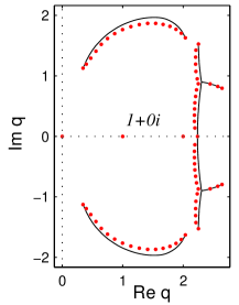
Figure 1: Chromatic roots for strip lattices. Red points: roots for a $4\times 18$ square lattice, free boundary conditions. Solid black line: limiting curve for a $4\times\infty$ lattice (again FBC).

3 Exploring the chromatic zeros of random graphs

To gain first insights toward chromatic zeros of random graphs, we consider the two models of the ER random graph [9]:

• $G(N,p)$: the graph has $N$ vertices, between every pair of vertices an edge exists with uniform probability $p$. The edge density $P$ of any individual instance will then vary normally around $p$.

• $G(N,M)$: the graph is chosen uniformly from all graphs with $N$ vertices and $M$ edges. The density $P$ then has the fixed value $M/\binom{N}{2}$.

In the $N\rightarrow\infty$ limit the two models are largely equivalent; for finite $N$ they can give different results, but the main reasons to use one or the other are practical. From the outset we had no clear idea of what to expect, so we began with a preliminary investigation of $G(N,p)$ graphs restricted to $N=20$. For each of the parameter values $p\in\{0.1,0.2,\dots,0.9\}$ we generated 20 sample graphs; we then calculated the chromatic polynomials with a Form [19] implementation of the new algorithm [17] and solved for the zeros of each polynomial numerically using MPSolve [2]. Complex zeros of all graphs plotted together are shown in figure 2(a). When first viewing these results we were struck by the distinct banding in both the horizontal and vertical directions, which implied that the complex zero sets could have a very predictable layout depending on the basic graph parameters. After confirming that similar patterns did not arise from zero sets of random polynomials with similar coefficients we proceeded to the second phase of our investigation, which was designed to measure the simultaneous effect of both edge-density and the number of vertices on the zero locations in a more systematic way.

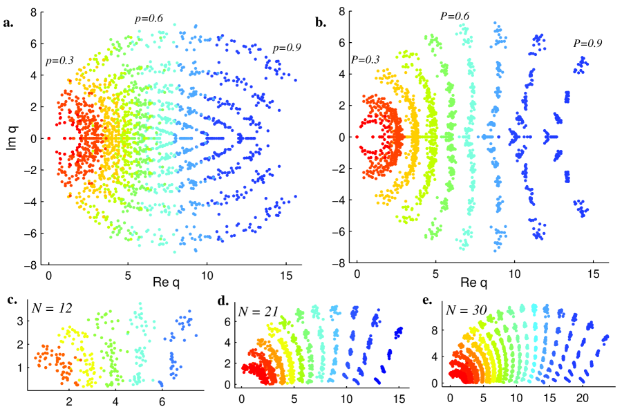
Figure 2: Complex zeros of chromatic polynomials of random graphs. (a) zeros for $G(20,p)$ with selection probability $p\in\{0.1,0.2,\dots,0.9\}$; (b) zeros for $G(20,M)$ graphs with $M$ determined by fixed edge density $P\in\{0.1,0.2,\dots,0.9\}$. (c), (d), and (e) zeros with positive real part for $G(N,M)$ graphs for selected $N$, $M=\left[KN/2\right]$ determined by the average degree $K\in\{3,4.5,6,\dots\}$. In all figures chromatic zeros for 20 sample graphs per parameter set are plotted together. Density is indicated by colour, running from red (low density) to blue (high density).

3.1 Parameters and constraints

In these more extensive investigations we consider the $G(N,M)$ instead of the $G(N,p)$ model. A cursory examination of the $G(20,p)$ data showed that the positions of chromatic zeros with non-zero imaginary part are very sensitive to the exact value of $P$, For example, within each $p$ group we found the correlation between the mean real value of these complex zeros and the exact $P$ value (as measured from counting the edges in the generated graphs) was between 0.982 and 0.994. Since we were interested in the effect of density on zero location we then decided to directly control for $P$. Figure 2(b) shows zero sets for fixed-density $G(N,M)$ graphs.

As well, we parameterized density by average degree $K=2M/N$ rather than directly by $P$, or by $M$. For a single value of $N$ it would not matter which of these was used, since they can be simply converted one to another, but over different $N$ the choice of metric affects the amount of data generated and the ways one can aggregate it. A deciding factor was that $K$ arises naturally in the study of physical systems which feature a bounded number of interactions.

Finally, we added the constraint that graphs were to be 2-connected: that is, every pair of vertices in the graph belong to at least one cycle. ER random graphs experience a sharp connectivity transition as density is increased [9]. Though the theoretical result is in the large $N$ limit, the effect is manifest even for $N$ in the range of the random graphs we used; none of our $G(20,0.1)$ graphs were even 1-connected, while all of the $G(20,p)$ graphs for $p\geq 0.3$ were at least 2-connected. Since the chromatic polynomial of an unconnected graph can be factorized into the chromatic polynomials of its connected components, aggregating data from graphs without controlling connectivity would have had the annoying effect of confounding the low-density data for runs with different values of $N$, without otherwise telling us anything we do not already know.

We used $N\in\{12,15,18,21,24,27,30\}$ and $K\in\{3,4.5,6,7.5,\dots,d\}$, where $d$ is highest value divisible by 1.5 that is less than $N-2$. For each of the 77 $(N,K)$ pairs 20 instances of $G(N,M)$ graphs were generated using the integer $M$ that was closest to $KN/2$. As above, chromatic polynomials were then calculated with the new algorithm and zeros extracted using MPSolve. Figure 2 (c), (d), and (e) show all chromatic zeros in the upper half complex plane for some $N$. Note that the upper value and spacing of the $N$ values chosen were primarily determined by computational concerns; for low $N$ chromatic polynomials for all graphs could be calculated in a matter of seconds, but in the high range a single graph could require two or more days. In total 1540 random graphs were generated, resulting in 35,700 individual data points (chromatic zeros).

3.2 Analysis of specific features of chromatic zeros

From the combined data we extracted various graph invariants directly, such as the chromatic number, number of real and integer zeros, zero multiplicities, the maximum modulus, maximum real zero, and maximum real and imaginary parts of zeros. Of particular interest to us were the shape traced out by the complex chromatic zero set (i.e. zeros with non-zero imaginary part) in the complex plane, and the point at which this set approaches closest to the real axis. The second of these we will denote as the crossing point $X_{N,r}$ for the parameter $r$ (which can be average degree $K$ or density $P$ as required).

The crossing point is a finite analogue to the critical value $q_{c}$ discussed by previous authors [15, 13, 5], which properly speaking can arise only in the $N\rightarrow\infty$ limit when critical phenomena arise, and the zero-set becomes continuous such that its intersection with the real axis can be solved explicitly. Since our graphs (and hence their chromatic zero sets) are finite the crossing points $X_{N,r}$ were instead estimated in the following way:

• For each parameter pair $(N,K)$ we collected the chromatic zeros with positive imaginary value for all 20 graphs into one set (zeros with negative imaginary value are their complex conjugates, and can thus be neglected);

• We fit an arc segment to each collected zero set in the complex plane; moreover, we did a linear fit to determine orientation (left or right leaning). All fits used least squares Euclidean distance from each zero to the nearest point on the arc (or line) as a metric. It should be noted here that centres and radii of arcs were not constrained in any way (for example, to lie on the real axis).

• The crossing point $X_{N,K}$ is then given by the positive intersection of the arc and the real axis. As well, the curvatures of the zero sets are obtained from the arc radii, and their orientations from the slopes of the linear fits.

4 Scaling of chromatic zeros

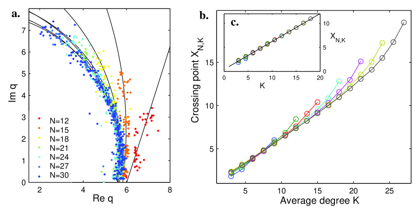
Figure 3: Crossing points for chromatic zero sets. (a) Complex chromatic zeros in upper half plane plus arc fits for average degree $K=9$, various $N$. (b) Crossing point $X_{N,K}$ vs. $K$ for each $N,K$. (c) (inset) Crossing points vs. average degree restricted to graphs with density $P<.65$ with fit line $X_{N,K}=0.58K+0.41$

Preliminary visual inspection of the complex chromatic zeros as shown in figure 2 revealed several consistent features. For all $N$ tested, the zero sets at low densities are close to the origin and laid out almost circularly around the point $1+0i$; as the density is increased they gradually move away from the origin and uncurl until they are almost vertical, after which the half-sets in the lower and upper complex plane remained relatively straight, but become shorter and angled, now away from the origin.

Perhaps most surprising is the way that zero sets for graphs with the same average degree $K$ almost always fell into roughly the same location regardless of the $N$ value. Figure 3(a) shows complex zeros for $K=9$. We note that the curvatures of these zero sets do vary, and that those of the smallest (hence densest) graphs pull to the right somewhat. Thus it would seem that while location and therefore crossing point is largely determined by average degree, features like the shape and height of the sets will depend on $P$ and $N$ in a more complex way.

The zero locations (see figure 3(b)) suggest that for random graphs with edge-density below a certain cutoff $P_{c}$ the crossing point $X_{N,K}$ scales linearly with $K$ but is otherwise insensitive to changes of $N$. As we will show below, it also turns out that $X_{N,K}$ has a predictable location for densities above $P_{c}$; in this range, however, it is no longer a linear function of $K$ but a still relatively simple function of $N$ and $P$. We remark that for low $K$ there is somewhat more variability in the data than elsewhere.

4.1 Determining cutoff density

By most measures the cutoff density $P_{c}$ is somewhere between 0.6 and 0.7. Though by no means conclusive, the best empirical metrics we have point to a value of $P_{c}\approx 0.65$. The most dispositive evidence involves the shape and orientation of the zero set. As we have noted, for a given $N$, as $K$ (or $P$) increases the shape of the zero set consistently goes from an arc curving around the origin to a pair of roughly straight lines leaning away from the origin. Our working assumption is thus that the cutoff should occur at the value of $K$ (or $P$) where the zero set is most vertical, simultaneously consistent with either a very large arc curling left or a straight line leaning imperceptibly right. This can be made more precise by considering the slopes of linear fits to the complex chromatic zero sets. For our data the slopes are negative for all zero sets with $P\leq 0.648$, and positive for all zero sets with $P\geq 0.652$ (no zero sets were associated with a density between these values).

4.2 Crossing point for $P<P_{c}$

Crossing points for $P<P_{c}$ exhibit a close to linear scaling with the average degree, cf. figure 3(c). Fitting $X_{N,K}$ against $K$ below the cutoff gives the relation as

$$X_{N,K}=0.582K+0.406.$$ (5)

Goodness of fit tests confirm that regardless of possible higher order terms the data points are aligned very closely to the fit line. The reduced chi-squared $\chi_{\textrm{r}}^{2}$ for the fit is a quite low 0.295 ($\chi_{\textrm{r}}^{2}$ is the standard $\chi^{2}$ normalized by the degrees of freedom; a value of one or less indicates that the model accounts for the data adequately or better, while values significantly greater than one mean the fit is of poor quality).

We note that the variability in measured data is greater for low $K$ values than for high. This is in part due to the fact that we have more low $K$ data points than high ones, and that variability of zero location is definitely greater at low densities (noticeable from simple visual inspection of zero plots). But there seems to be another factor at work as well. For individual $N$ values the differences between the calculated $X_{N,K}$ values and the fit are not scattered about the line, but instead are larger (and consistently positive) towards both ends of the applicable density range. As well, the crossing point for $K=2$ (a cycle) should be at $Re(q)=2$, while the fit line predicts a too-low value of 1.57. This may imply that actual curves are either very gently rounded, or that there is a separate low density regime where a different slope applies. We do not currently have any good criterion for distinguishing a second cutoff, however. Moreover, the magnitude of these differences is small, and does not seem to increase with larger $N$.

4.3 Crossing point for $P>P_{c}$

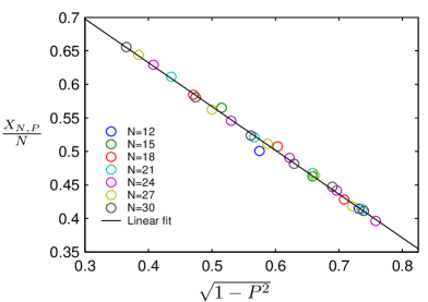
Figure 4: Rescaled crossing points $X_{N,P}/N$ vs. $\sqrt{1-P^{2}}$, $P>P_{c}$

The crossing points above the cutoff density do not scale directly with $K$; in fact, it is not clear from visual inspection that they conform to any simple function of $K$ or $P$. Hence it is something of a surprise to find out that for $P>P_{c}$ the crossing points are rather well described by

$$X_{N,P}=N\left(a-b\sqrt{1-P^{2}}\right),$$ (6)

where $a\approx 0.9$ and $b\approx 0.65\approx P_{c}$, as shown in figure 4. This relation was obtained by considering a rescaling of the crossing point values to correct for the fact that the distance from the cutoff crossing point $X_{N,P_{c}}$ to $N$ increases as roughly $0.4N$ with $N$. It turned out that when rescaled this way the $X_{N,P}$ values for different $N$ fell close to the same arc segment when plotted against $P$; hence the $\sqrt{1-P^{2}}$ term in the relation above. The exact linear fit has a $\chi_{\textrm{r}}^{2}$ of 0.2868.

4.4 Further quantities of interest

As mentioned above, we have considered a large number of other quantities of interest. Each of these quantities requires a thorough scaling analysis on its own, such that we here give only a brief summary of the most important results and refer the reader to an extensive presentation in a future publication. The maximum zero modulus $|z_{max}|$ and the maximum imaginary value $\max(Im(z))$ both as well turn out to have simpler scalings than were anticipated. The maximum modulus is well approximated across all densities by the linear relation

$$|z_{max}|=0.91K-0.79$$ (7)

though the exact relation again is probably non-linear at least in the high and low density range; while all points are close to the fit line the errors are not scattered normally but definitely pull up at both ends (cf. figure 5). The maximum imaginary value does not grow linearly with $K$, but a linear relation can be obtained by rescaling:

$$\max(Im(z))=1.15K\sqrt{1-P}-1.67.$$ (8)

A $\chi_{\textrm{r}}^{2}$ value of 0.296 again confirms a high quality fit. Since $K=P(N-1)$, for fixed $P$ this relation does give a linear scaling, this time in $N$. We note that $P\sqrt{1-P}$ achieves its maximum at $P=\frac{2}{3}$; hence this result dovetails with our finding of the density cutoff for the crossing point scaling at $P_{c}\approx 0.65$, based on the most vertical layout of the chromatic zero set.

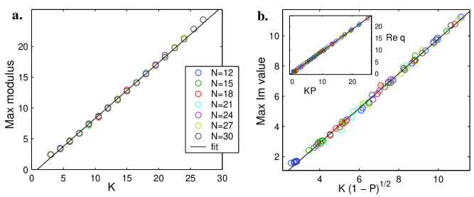
Figure 5: (a) Maximum modulus (mean over each $N,K$ parameter set) vs. average degree $K$. (b) Maximum imaginary value (mean over each $N,K$ parameter set) vs. $K\sqrt{1-P}$. Inset shows associated real values vs. $KP$.

5 Conclusions

Applying the recently suggested vertex-based computational method [17] yielded some corner-stone insights into the features of chromatic polynomials of random graphs: the complex zeros of chromatic polynomials of moderately sized random graphs systematically change with the number of vertices $N$, the density $P$ and the average degree $K$. For fixed $N$ the shapes of the complex zero sets evolve as $P$ increases, from tracing an arc around the point $1+0i$ at low $P$, to being almost vertically aligned at the cutoff density $P_{c}\approx 0.65$, to sitting along pairs of straight lines leaning away from the origin at higher $P$. The crossing point $X_{N,K}$ of the complex zeros scales linearly with the average degree $K$ for $P<P_{c}$; above this cutoff the crossing point appears to be a simple function of $N$ and $\sqrt{1-P^{2}}$. If these results continue to hold for larger $N$, the implications are straightforward. Fixing the average degree $K$, we have $P\rightarrow 0$ as $N\rightarrow\infty$; this suggests that for an infinite random graph with bounded degree the chromatic zero set converges to an arc around $1+0i$ that crosses the real axis at a finite position. On the other hand, if $P$ is fixed or converges to a positive value then $K\rightarrow\infty$ and the crossing point and in fact all chromatic zeros with non-zero imaginary value diverge to (complex) infinity. The former is most relevant for statistical physics: if $G$ is an infinite disordered system with bounded connectivity then in the zero-temperature limit the zeros of antiferromagnetic Potts partition function meet the real axis at a finite, predictable location that depends on the system’s coordination number.

Besides extending our studies to related polynomials such as Tutte or reliability polynomials [6, 18], the chromatic polynomial itself requires several future studies. In particular, there is of course much that still needs to be done with respect to Erdös-Rényi random graphs. Ideally we would like to obtain results for larger $N$ for additional verification. However, while the new method [17] does achieve a significant speedup, the problem of computing the chromatic polynomial remains difficult and so there is a limit to feasible $N,P$ values.

Nevertheless, even for accessible classes of graphs, several features of their chromatic polynomials are not yet settled: While our results indicate that for ER random graphs the location of chromatic zeros may be quite predictable, there are many related graphs of interest with as yet unknown features. Preliminary studies on two other classes of graphs, regular random graphs and random bipartite graphs, suggest how far and in what direction our current results might extend. As one might expect, with respect to regular random graphs the main effect is to reduce the variation in zero location across instances. The layout of the chromatic zero sets for random bipartite graphs, on the other hand, is markedly different than what we see for general ER random graphs, particularly at higher densities. Since many lattices are as well bipartite this bears closer study.

Two further ‘standard’ classes of networks and graphs include:
—Small-world graphs. There is a possibility that our scalings may depend on properties that will almost always hold for small enough random graphs yet almost never hold for large enough ones. One such property relates to the presence of triangles and other small cycles. None of our graphs with average degree more than three were triangle free, though for densities $P<1$ large enough random graphs will usually be triangle free, and infinite random graphs are locally indistinguishable from trees. Small-world graphs [20], which maintain their neighborhood properties as they grow larger, are hence natural candidates for study.
—Scale-free networks. Some previous work on chromatic polynomials has brought up the possibility that the presence of high degree vertices may have a large influence on the location of some of the graph’s chromatic zeros [16]. We have not detected a pronounced effect coming from the maximum degree itself but this might be due to the strongly central, unimodal distribution of the degrees for the random graphs we considered. Hence it is entirely possible that the non-effect we noticed is due to our maximum degrees not being large enough compared to the average degrees to exert an independent influence. To test this supposition, a natural option would be to compute chromatic zeros of graphs with scale-free degree distributions. The vertex-based symbolic method we used [17] would need to be adapted to compute reasonable size instances.

References

- [1] R. Baxter, Exactly solved models in statistical mechanics. London: Academic Press Inc. (1982)
- [2] D. Bini and G. Fiorentino, Design, Analysis, and Implementation of a Multiprecision Polynomial Rootfinder, Numerical Algorithms 23 127–173 (2000)
- [3] G. Birkhoff, A Determinant Formula for the Number of Ways of Coloring a Map, Ann. Math. 14 42–46 (1912)
- [4] B. Bollobás, The Chromatic Number of Random Graphs, Combinatorica 8 49–55 (1988)
- [5] S.-C. Chang and R. Shrock, Ground State Entropy of the Potts Antiferromagnet on Strips of the Square Lattice, Physica A 290 402–430 (2001)
- [6] S.-C. Chang and R. Shrock, Reliability Polynomials and Their Asymptotic Limits for Families of Graphs, J. Stat. Phys. 112 1019–1077 (2003)
- [7] A. Hartmann and M. Weigt, Phase Transitions in Combinatorial Optimization Problems. New York: Wiley-VCH (2005)
- [8] K. Huang, Statistical Mechanics. New York: John Wiley & Sons (1987)
- [9] S. Janson, T. Łuczak and A. Rucinski, Random Graphs. New York: John Wiley & Sons (2000)
- [10] T. Lee and C. Yang, Statistical Theory of Equations of State and Phase Transitions. II. Lattice Gas and Ising Model, Phys. Rev. 87, 410–419 (1952)
- [11] L. Onsager, Crystal Statistics. I. A Two-Dimensional Model with an Order-Disorder Transition, Phys. Rev. 65, 117–149 (1944)
- [12] R. Potts, Some Generalized Order-Disorder Transformations, Proc. Camb. Phil. Soc. 48 106 (1952)
- [13] M. Roček, R. Shrock and S.-H. Tsai, Chromatic polynomials for families of strip graphs and their asymptotic limit, Physica A 252 505–546 (1998)
- [14] J. Salas and A. Sokal, Transfer Matrices and Partition-Function Zeros for Antiferromagnetic Potts Models. I. General Theory and Square-Lattice Chromatic Polynomial, J. Stat. Phys. 104 609–699 (2001)
- [15] R. Shrock and S.-H. Tsai, Asymptotic Limits and Zeros of Chromatic Polynomials and Ground-State Entropy of Potts Antiferromagnets, Phys. Rev. E 55 5165–5178 (1997)
- [16] A. Sokal, Chromatic Polynomials, Potts Models and All That, Physica A 279 324–332 (2000)
- [17] M. Timme, F. Van Bussel, D. Fliegner and S. Stolzenberg, Solving Hard Counting Problems by Efficient Pattern Matching: Chromatic Polynomials and Potts Partition Function, New J. Phys. 11 023001 (2009)
- [18] W. Tutte, A Contribution to the Theory of Chromatic Polynomials, Can. J. Math. 6 80–91 (1954)
- [19] J. Vermaseren, New features of FORM, arXiv math-ph/0010025v2 (2000)
- [20] D. Watts and S. Strogatz, Collective dynamics of “small-world” networks, Nature 393 440–442 (1998)
- [21] H. Wilf, Algorithms and Complexity. Englewood Cliffs, NJ: Prentice-Hall (1986)
- [22] F. Wu, The Potts model, Rev. Mod. Phys. 54, 235–268 (1982)