Synchronization Patterns in Networks of Kuramoto Oscillators:
A Geometric Approach for Analysis and Control

Abstract

Synchronization is crucial for the correct functionality of many natural and man-made complex systems. In this work we characterize the formation of synchronization patterns in networks of Kuramoto oscillators. Specifically, we reveal conditions on the network weights and structure and on the oscillators’ natural frequencies that allow the phases of a group of oscillators to evolve cohesively, yet independently from the phases of oscillators in different clusters. Our conditions are applicable to general directed and weighted networks of heterogeneous oscillators. Surprisingly, although the oscillators exhibit nonlinear dynamics, our approach relies entirely on tools from linear algebra and graph theory. Further, we develop a control mechanism to determine the smallest (as measured by the Frobenius norm) network perturbation to ensure the formation of a desired synchronization pattern. Our procedure allows us to constrain the set of edges that can be modified, thus enforcing the sparsity structure of the network perturbation. The results are validated through a set of numerical examples.

I Introduction

Synchronization of coupled oscillators is everywhere in nature [1, 2, 3] and in several man-made systems, including power grids [4] and computer networks [5]. While some systems require complete synchronization among all the parts to function properly [6, 7], others rely on cluster or partial synchronization [8], where subsets of nodes exhibit coherent behaviors that remain independent from the evolution of other oscillators in the network. For example, while partial synchronization patterns have been observed in healthy individuals [9], complete synchronization in neural systems is associated with degenerative diseases including Parkinson’s and Huntington’s diseases [10, 11], and epilepsy [12]. Cluster synchronization has received attention only recently, and several fundamental questions remain unanswered, including the characterization of the network features enabling the formation of a desired pattern, and the development of control mechanisms to enforce the emergence of clusters.

In this paper we focus on networks of Kuramoto oscillators [13], and we characterize intrinsic and topological conditions that ensure the formation of desired clusters of oscillators. Our network model is motivated by a large body of literature showing broad applicability of the Kuramoto model to virtually all systems that exhibit synchronization properties. Although Kuramoto networks exhibit nonlinear dynamics, we adopt tools from linear algebra and graph theory to characterize network conditions enabling the formation of a given synchronization pattern. Further, we design a control mechanism to perturb (a subset of) the network weights so as to enforce or prevent desired synchronization patterns.

Related work Complete synchronization in networks of Kuramoto oscillators has been extensively studied, e.g., see [14, 15]. It has been shown that synchronization of all nodes emerges when the coupling strength among the agents is sufficiently larger than the heterogeneity of the oscillators’ natural frequencies. Partial synchronization and pattern formation have received considerably less attention, with the literature being composed of only few recent works. In [16] it is shown how symmetry of the interconnections may lead to partial synchronization. Methods based on graph symmetry have also been used to find all possible clusters in networks of Laplacian-coupled oscillators [17]. The relationship between clusterization and network topology has been studied in [18] for unweighted interconnections. In [19], the emergence and the stability of groups of synchronized agents within a network has been studied for different classes of dynamics, like delay-coupled laser models and neuronal spiking models. Here, the approach of master stability function has been used to characterize the results. In [20, 21] the idea is put forth to study an approximate notion of cluster synchronization in Kuramoto networks via tools from linear systems theory. It is quantitatively shown how cluster synchronization depends on strong intra-cluster and weak inter-cluster connections, similarity with respect to the natural frequencies of the oscillators within each cluster, and heterogeneity of the natural frequencies of coupled oscillators belonging to different subnetworks. With respect to this work, we focus on an exact notion of cluster synchronization, identify necessary and sufficient conditions on the network weights and oscillators’ natural frequencies for the emergence of a desired synchronization pattern, and exploit our analysis to design a structural control algorithm for the formation of a desired synchronization pattern.

The work that is closer to this paper is [22], where the authors relate cluster synchronization to the notion of an external equitable partition in a graph. In fact, the notion of an external equitable partition can be interpreted in terms of invariant subspaces of the network adjacency matrix, a notion that we exploit in our development. However, the analysis in [22] is carried out with unweighted and undirected networks and, as we show in this paper, the conditions in [22] may not be necessary when dealing with directed and weighted networks. Further, our approach relies on simple notions from linear algebra, and leads to the development of our control algorithm for the formation of desired patterns.

Paper contributions The contributions of this paper are twofold. First, we consider a notion of exact cluster synchronization, where the phases of the oscillators within each cluster remain equal to each other over time, and different from the phases of the oscillators in different clusters. We derive necessary and sufficient conditions for the formation of a given synchronization pattern in directed and weighted networks of Kuramoto oscillators. In particular we show that cluster synchronization is possible if and only if (i) the natural frequencies are equal within each cluster, and (ii) for each cluster, the sum of the weights of the edges from every separate group is the same for all nodes in the cluster. Second, we leverage our characterization of cluster synchronization to develop a control mechanism that modifies the network weights so as to ensure the formation of a desired synchronization pattern. Our control method is optimal, in the sense that it determines the smallest (measured by the Frobenius norm) network perturbation for a given synchronization pattern, and it guarantees the modification of only a desired subset of the edge weights.

Paper organization The rest of this paper is organized as follows. Section II contains the problem setup and some preliminary definitions. Section III contains our characterization of cluster synchronization, and Section IV contains our structural control algorithm for the formation of a desired synchronization pattern. Section V concludes the paper.

II Problem setup and preliminary notions

Consider a network of heterogenous Kuramoto oscillators described by the digraph $\mathcal{G}=(\mathcal{V},\mathcal{E})$, where $\mathcal{V}=\{1,\dots,n\}$ denotes the set of oscillators and $\mathcal{E}\subseteq\mathcal{V}\times\mathcal{V}$ their interconnections. Let $A=[a_{ij}]$ be the weighted adjacency matrix of $\mathcal{G}$, where $a_{ij}\in$ if $(i,j)\in\mathcal{E}$ and $a_{ij}=0$ otherwise. We assume that $\mathcal{G}$ is strongly connected [23]. Let $\theta_{i}\in\mathbb{R}$ denote the phase of the $i$-th oscillator, whose dynamics reads as

$$\dot{\theta}_{i}=\omega_{i}+\sum_{j=1}^{n}a_{ij}\sin(\theta_{j}-\theta_{i}),$$

where $\omega_{i}$ is the natural frequency of the $i$-th oscillator. The dynamics is a generalized version of the classic Kuramoto model [24]. Depending on the interconnection graph $\mathcal{G}$, the adjacency matrix $A$, and the oscillators natural frequencies, different oscillatory patterns are possible corresponding to (partially) synchronized or chaotic states [25]. In this work we are particularly interested in the case where the phases of groups of oscillators evolve cohesively within each group, yet independently from the phases of oscillators in different groups. To formalize this discussion, let $\mathcal{P}=\{\mathcal{P}_{1},\dots,\mathcal{P}_{m}\}$ be a partition of $\mathcal{V}$, that is, $\mathcal{V}=\cup_{i=1}^{m}\mathcal{P}_{i}$ and $\mathcal{P}_{i}\cap\mathcal{P}_{j}=\emptyset$ for all $i,j\in\{1,\dots,m\}$ with $i\neq j$. We restrict our attention to the case $m>1$. Throughout the paper we will assume without loss of generality that, given $\mathcal{P}=\{\mathcal{P}_{1},\dots,\mathcal{P}_{m}\}$, the oscillators are labeled so that $\mathcal{P}_{i}=\{\sum_{j=1}^{i-1}|\mathcal{P}_{j}|+1,\dots,\sum_{j=1}^{i}|\mathcal{P}_{j}|\}$, where $|\mathcal{P}_{j}|$ denotes the cardinality of the set $\mathcal{P}_{j}$. While different notions of synchronization exist, we will use the following definitions.

Definition 1

(Phase synchronization) For the network of oscillators $\mathcal{G}=(\mathcal{V},\mathcal{E})$, the partition $\mathcal{P}=\{\mathcal{P}_{1},\dots,\mathcal{P}_{m}\}$ is phase synchronizable if, for some initial phases $\theta_{1}(0),\dots,\theta_{n}(0)$, it holds

$$\theta_{i}(t)=\theta_{j}(t),$$

for all times $t\in_{\geq 0}$ and $i,j\in\mathcal{P}_{k}$, with $k\in\{1,\dots,m\}$. $\square$

Definition 2

(Frequency synchronization) For the network of oscillators $\mathcal{G}=(\mathcal{V},\mathcal{E})$, the partition $\mathcal{P}=\{\mathcal{P}_{1},\dots,\mathcal{P}_{m}\}$ is frequency synchronizable if, for some initial phases $\theta_{1}(0),\dots,\theta_{n}(0)$, it holds

$$\dot{\theta}_{i}(t)=\dot{\theta}_{j}(t),$$

for all times $t\in_{\geq 0}$ and $i,j\in\mathcal{P}_{k}$, with $k\in\{1,\dots,m\}$. $\square$

Clearly, phase synchronization implies frequency synchronization, while the converse statement typically fails to hold.

Finally, we define the characteristic matrix associated with a partition $\mathcal{P}$ of the network nodes, which will be used to derive our synchronization conditions in Section III.

Definition 3

(Characteristic matrix) For the network of oscillators $\mathcal{G}=(\mathcal{V},\mathcal{E})$ and the partition $\mathcal{P}=\{\mathcal{P}_{1},\dots,\mathcal{P}_{m}\}$, the characteristic matrix of $\mathcal{P}$ is $V_{\mathcal{P}}\in^{n\times m}$, where

$$V_{\mathcal{P}}=\begin{bmatrix}v_{1}&v_{2}&\cdots&v_{m}\end{bmatrix},$$

and

$$v_{i}^{\mathsf{T}}=\big{[}\underbrace{\begin{matrix}0&0&\cdots&0\end{matrix}}_{\sum_{j=1}^{i-1}|\mathcal{P}_{j}|}\;\underbrace{\begin{matrix}1&1&\cdots&1\end{matrix}}_{|\mathcal{P}_{i}|}\;\underbrace{\begin{matrix}0&0&\cdots&0\end{matrix}}_{\sum_{j=i+1}^{n}|\mathcal{P}_{j}|}\big{]}.$$

$\square$

We conclude this section with an illustrative example.

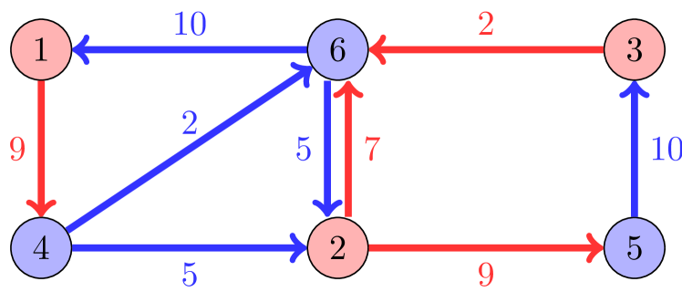
Figure 1: A network of oscillators with partitions $\mathcal{P}_{1}=\{1,2,3\}$ and $\mathcal{P}_{2}=\{4,5,6\}$. The sum of the weights of all edges $(i,j)$ is equal for each node $i$ of $\mathcal{P}_{1}$ (resp. $\mathcal{P}_{2}$), with $j\in\mathcal{P}_{2}$ (resp. $j\in\mathcal{P}_{1}$). In Section III we show that this is a necessary condition for phase synchronization of the partition $\mathcal{P}$.

Example 1

(Setup and definitions) Consider the network of Kuramoto oscillators in Fig. 1, with graph $\mathcal{G}=(\mathcal{V},\mathcal{E})$, $\mathcal{V}=\{1,2,3,4,5,6\}$ and partition $\mathcal{P}=\{\mathcal{P}_{1},\mathcal{P}_{2}\}$. The graph $\mathcal{G}$ and the partition $\mathcal{P}$ are described by $A$ and $V_{\mathcal{P}}$ as follows:

$$A=\begin{bmatrix}0&0&0&0&0&10\\ 0&0&0&5&0&5\\ 0&0&0&0&10&0\\ 9&0&0&0&0&0\\ 0&9&0&0&0&0\\ 0&7&2&2&0&0\end{bmatrix},V_{\mathcal{P}}=\begin{bmatrix}1&0\\ 1&0\\ 1&0\\ 0&1\\ 0&1\\ 0&1\end{bmatrix}.$$

$\square$

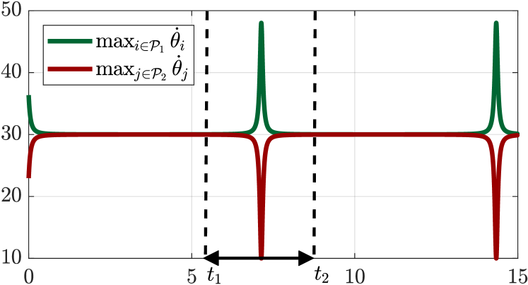
Figure 2: For the network in Example 1 with natural frequencies $\omega=[30,30,30,10,10,10]^{\mathsf{T}}$ Fig. (a) shows the frequencies of the oscillators in the clusters $\mathcal{P}_{1}=\{1,2,3\}$ and $\mathcal{P}_{2}=\{4,5,6\}$ as a function of time. Notice that Assumption A1 is satisfied over the entire time interval. In Fig. (b) we let the frequencies be more homogeneous, $\omega=[19,19,19,10,10,10]^{\mathsf{T}}$. Assumption A1 is satisfied within bounded time intervals, such as $[t_{1},t_{2}]$.

III Conditions for cluster synchronization

In this section we derive necessary and sufficient conditions ensuring phase (hence frequency) synchronization of a partition of oscillators. In particular, we show how synchronization of a partition depends both on the interconnection structure and weights, as well as the oscillators natural frequencies. We make the following technical assumption.

• For the partition $\mathcal{P}=\{\mathcal{P}_{1},\dots,\mathcal{P}_{m}\}$ there exists an ordering of the clusters $\mathcal{P}_{i}$ and an interval of time $[t_{1},t_{2}]$, with $t_{2}>t_{1}$, such that for all times $t\in[t_{1},t_{2}]$:

  $$\max_{i\in\mathcal{P}_{1}}\dot{\theta}_{i}>\max_{i\in\mathcal{P}_{2}}\dot{\theta}_{i}>\cdots>\max_{i\in\mathcal{P}_{m}}\dot{\theta}_{i}.$$

Assumption (A1) requires the phases of the oscillators in different clusters to evolve with different frequencies, at least in some interval of time. This assumption is in fact not restrictive, as this is typically the case when the oscillators in different clusters have different natural frequencies. Two cases where this assumption is satisfied are presented in Fig. 2. A special case where Assumption (A1) is not satisfied is discussed at the end of this section.

Theorem III.1

(Cluster synchronization) For the network of oscillators $\mathcal{G}=(\mathcal{V},\mathcal{E})$, the partition $\mathcal{P}=\{\mathcal{P}_{1},\dots,\mathcal{P}_{m}\}$ is phase synchronizable if and only if the following conditions are simultaneously satisfied:

1. the network weights satisfy $\sum_{k\in\mathcal{P}_{\ell}}a_{ik}-a_{jk}=0$ for every $i,j\in\mathcal{P}_{z}$ and $z,\ell\in\{1,\dots,m\}$, with $z\neq\ell$;

2. the natural frequencies satisfy $\omega_{i}=\omega_{j}$ for every $k~{}\in~{}\{1,\dots,m\}$ and $i,j\in\mathcal{P}_{k}$.

Proof:

(If) Let $\theta_{i}=\theta_{j}$ for all $i,j\in\mathcal{P}_{k}$, $k=1,\dots,m$. Let $i,j\in\mathcal{P}_{\ell}$, and notice that

$$\dot{\theta}_{i}-\dot{\theta}_{j} =\sum_{z\neq\ell}\sum_{k\in\mathcal{P}_{z}}a_{ik}\sin(\theta_{k}-\theta_{i})-a_{jk}\sin(\theta_{k}-\theta_{j})$$

$$=\sum_{z\neq\ell}s_{z\ell}\sum_{k\in\mathcal{P}_{z}}a_{ik}-a_{jk}=0,$$

where we have used conditions (i) and (ii), and where $s_{zl}=\sin(\theta_{z}-\theta_{\ell})$ depends on the clusters $z$ and $\ell$ but not on $i,j,k$. Thus, when conditions (i) and (ii) are satisfied, $\theta\in\operatorname{Im}(V_{\mathcal{P}})$ implies $\dot{\theta}\in\operatorname{Im}(V_{\mathcal{P}})$, the image of $V_{\mathcal{P}}$. $\operatorname{Im}(V_{\mathcal{P}})$ is invariant and the network is phase synchronizable ($\theta(0)\in\operatorname{Im}(V_{\mathcal{P}})$).

(Only if) We first show that condition (i) is necessary for phase synchronization. Assume that the network is phase synchronized. Let $i,j\in\mathcal{P}_{\ell}$. At all times is must hold that

$$\begin{split}0=\ddot{\theta}_{i}-\ddot{\theta}_{j}=&\sum_{z\neq\ell}\sum_{k\in\mathcal{P}_{z}}a_{ik}\cos(\theta_{k}-\theta_{i})(\dot{\theta}_{k}-\dot{\theta}_{i})\\ &-\sum_{z\neq\ell}\sum_{k\in\mathcal{P}_{z}}a_{jk}\cos(\theta_{k}-\theta_{j})(\dot{\theta}_{k}-\dot{\theta}_{j})\\ &=\sum_{z\neq\ell}c_{z\ell}v_{z\ell}\underbrace{\sum_{k\in\mathcal{P}_{z}}a_{ik}-a_{jk}}_{d_{z}},\end{split}$$ (1)

where $c_{z\ell}=\cos(\theta_{z}-\theta_{\ell})$ and $v_{z\ell}=\dot{\theta}_{z}-\dot{\theta}_{\ell}$ depend on the clusters $z$ and $\ell$, but not on $i,j,k$. From (A1), possibly after reordering the clusters, in some nontrivial interval we have

$$\max_{i\in\mathcal{P}_{1}}\dot{\theta}_{i}>\max_{i\in\mathcal{P}_{2}}\dot{\theta}_{i}>\cdots>\max_{i\in\mathcal{P}_{m}}\dot{\theta}_{i}.$$

Thus, (1) implies that, either $d_{z}=0$ for all $z$ (thus implying condition (i)), or the functions $c_{z\ell}v_{z\ell}$ must be linearly dependent at all times in the interval. Assume by contradiction that the functions $c_{zl}v_{zl}$ are linearly dependent at all times in the above interval. Then it must hold that

$$\sum_{z\neq\ell}d_{z}\frac{d^{n}}{dt^{n}}c_{z\ell}v_{z\ell}=0,$$

for every nonnegative integer $n$, where $\frac{d^{n}}{dt^{n}}$ denotes $n$-times differentiation. In other words, not only the functions $c_{z\ell}v_{z\ell}$ must be linearly dependent, but also all their derivatives, at some times in the above interval. Let $d_{1}\neq 0$ (if $d_{1}=0$, simply select the first nonzero coefficient), and $i,j\not\in\mathcal{P}_{1}$. Because of assumption (A1), there exists an integer $n$ such that $d_{1}\frac{d^{n}}{dt^{n}}c_{1\ell}v_{1\ell}\gg d_{z}\frac{d^{n}}{dt^{n}}c_{z\ell}v_{z\ell}$, for all $z\neq 1$. Thus, the functions $c_{z\ell}v_{z\ell}$ cannot be linearly dependent. We conclude that statement (i) is necessary for phase synchronization.

We now prove that, when the network is phase synchronized, statement (i) implies statement (ii). This shows that statement (ii) is necessary for phase synchronization. Let the network be phase synchronized, and let $i,j\in\mathcal{P}_{\ell}$. We have

$$0=\dot{\theta}_{i}-\dot{\theta}_{j}=\omega_{i}-\omega_{j}+\sum_{z\neq\ell}s_{z\ell}\underbrace{\sum_{k\in\mathcal{P}_{z}}a_{ik}-a_{jk}}_{=0},$$

where $s_{z\ell}=\sin(\theta_{z}-\theta_{\ell})$ does not depend on the indices $i,j,k$ (see above), and where we have used that statement (i) is necessary for phase synchronization. To conclude, $\omega_{i}=\omega_{j}$, and statement (ii) is also necessary for phase synchronization. ∎

Remark 1

(Necessity of assumption A1) Consider a network of oscillators with adjacency matrix

$$A=\begin{bmatrix}0&a_{12}&0&0\\ a_{21}&0&a_{23}&0\\ 0&a_{32}&0&a_{34}\\ 0&0&a_{43}&0\\ \end{bmatrix},$$

and natural frequencies $\omega_{i}=\bar{\omega}$ for all $i\in\{1,\dots,4\}$. Notice that condition (i) in Theorem III.1 is not satisfied. Let $\theta_{1}(0)=\theta_{2}(0)$ and $\theta_{3}(0)=\theta_{4}(0)=\theta_{1}(0)+\pi$, and notice that $\dot{\theta}_{i}=\bar{\omega}$ at all times and for all $i\in\{1,\dots,4\}$ (Assumption A1 is not satisfied). In other words, the partition $\mathcal{P}=\{\mathcal{P}_{1},\mathcal{P}_{2}\}$, with $\mathcal{P}_{1}=\{1,2\}$ and $\mathcal{P}_{2}=\{3,4\}$ is phase synchronized, independently of the interconnection weights among the oscillators. Thus, condition (i) in Theorem may not be necessary when Assumption A1 is not satisfied. $\square$

Let $A\odot B$ denote the Hadamard product between $A$ and $B$ [26], and $\operatorname{Im}(V_{\mathcal{P}})^{\perp}$ the orthogonal subspace to $\operatorname{Im}(V_{\mathcal{P}})$.

Corollary III.2

(Matrix condition for synchronization) Condition $(i)$ in Theorem III.1 is equivalent to $\bar{V}_{\mathcal{P}}^{\mathsf{T}}\bar{A}V_{\mathcal{P}}=0$, where $\bar{V}_{\mathcal{P}}\in\mathbb{R}^{n\times(n-m)}$ satisfies $\operatorname{Im}(\bar{V}_{\mathcal{P}})=\operatorname{Im}(V_{\mathcal{P}})^{\perp}$, and

$$\bar{A}=A-A\odot V_{\mathcal{P}}V_{\mathcal{P}}^{\mathsf{T}}.$$ (2)

Proof:

Let $\bar{A}=[\bar{a}_{ij}]$ and $A=[a_{ij}]$. Notice that $\bar{a}_{ij}=a_{ij}$ when $i$ and $j$ belong to different clusters, and $\bar{a}_{ij}=0$ when $i$ and $j$ belong to the same cluster. Thus,

$$[\bar{A}V_{\mathcal{P}}]_{ij}=\begin{cases}\sum_{k\in\mathcal{P}_{j}}a_{ik},&\text{if }i\notin\mathcal{P}_{j},\\ 0,&\text{if }i\in\mathcal{P}_{j}.\end{cases}$$

Select $\bar{V}_{\mathcal{P}}$ so that $\bar{V}_{\mathcal{P}}=[\bar{v}_{1}\cdots\bar{v}_{n-m}]$ and $\bar{v}_{i}^{\mathsf{T}}x=x_{r}-x_{s}$, with $r,s\in\mathcal{P}_{\ell}$, for a vector $x$ of compatible dimension. Then,

$$[\bar{V}_{\mathcal{P}}^{\mathsf{T}}\bar{A}V_{\mathcal{P}}]_{ij}=\begin{cases}\sum_{k\in\mathcal{P}_{j}}a_{rk}-a_{sk},&r,s\notin\mathcal{P}_{j},\\ 0,&r,s\in\mathcal{P}_{j},\end{cases}$$

where $r,s$ are the nonzero indices of $\bar{v}_{i}$. ∎

IV Control of cluster synchronization

In the previous section we derive conditions on the network of oscillators to guarantee phase and frequency synchronization. These conditions are rather stringent, and are typically not satisfied for arbitrary partitions and interconnection weights. In this section we develop a control mechanism to modify the oscillators’ interconnection weights so as to guarantee synchronization of a given partition. Specifically, we study the following minimization problem:

$$\min_{\Delta}\;\;\;\;\;\; \|\Delta\|^{2}_{F}$$ (3a)

s.t. $$\bar{V}_{\mathcal{P}}^{\mathsf{T}}\left[\bar{A}+\Delta\right]V_{\mathcal{P}}=0$$ (3b)

$$\Delta\in\mathcal{H}$$ (3c)

where $\|\Delta\|_{F}$ denotes the Frobenius norm of the matrix $\Delta$, $\bar{A}$ is as in (2), and $\mathcal{H}$ encodes a desired sparsity pattern of the perturbation matrix $\Delta$. For example, $\mathcal{H}$ may represent the set of matrices compatible with the graph $\mathcal{G}=(\mathcal{V},\mathcal{E})$, that is, $\mathcal{H}=\{M\;:\;M\in^{|\mathcal{V}|\times|\mathcal{V}|}\text{ and }m_{ij}=0\text{ if }(i,j)\not\in\mathcal{E}\}$. The constraint (3b) reflects the invariance condition in Corollary III.2 and, together with condition (ii) in Theorem III.1, ensures synchronization of the partition $\mathcal{P}$. Thus, the minimization problem (3) determines the smallest perturbation of the interconnection weights that guarantees synchronization of a partition $\mathcal{P}$ and satisfies desired sparsity constraints. It should be observed that, given the solution $\Delta^{*}$ to (3), the modified adjacency matrix is $A+\Delta^{*}$ even if the constraint (3b) is expressed in terms of $\bar{A}$. This follows from the fact that connections among nodes of the same cluster do not affect the synchronization properties of the partition $\mathcal{P}=\{\mathcal{P}_{1},\dots,\mathcal{P}_{m}\}$ (see Corollary III.2).

To solve the minimization problem (3), we define the following minimization problem by including the sparsity constraints (3c) into the cost function:

$$\min_{\Delta}\;\;\;\;\;\; \|\Delta\oslash H\|^{2}_{F}$$ (4a)

s.t. $$\bar{V}_{\mathcal{P}}^{\mathsf{T}}\left[\bar{A}+\Delta\right]V_{\mathcal{P}}=0$$ (4b)

where $\oslash$ denotes elementwise division, and $H$ satisfies $h_{ij}=1$ if there exists a matrix $M\in\mathcal{H}$ such that $m_{ij}\neq 0$, and $h_{ij}=0$ otherwise. Clearly, the minimization problems (3) and (4) are equivalent, in the sense that $\Delta^{*}$ is a (feasible) solution to (3) if and only if it has finite cost in (4).

Theorem IV.1

(Synchronization via structured perturbation) Let $T=[V_{\mathcal{P}}\;\bar{V}_{\mathcal{P}}]$, and let

$$\begin{bmatrix}\tilde{A}_{11}&\tilde{A}_{12}\\ \tilde{A}_{21}&\tilde{A}_{22}\end{bmatrix}=T^{-1}\bar{A}T.$$

The minimization problem (3) has a solution if and only if there exists a matrix $\Lambda$ satisfying

$$X =(\bar{V}_{\mathcal{P}}\Lambda V_{\mathcal{P}}^{\mathsf{T}})\odot H,\text{ and }\tilde{A}_{21}=\bar{V}_{\mathcal{P}}^{\mathsf{T}}XV_{\mathcal{P}}.$$

Moreover, if it exists, a solution $\Delta^{*}$ to (3) is

$$\Delta^{*}=T\begin{bmatrix}\tilde{\Delta}_{11}^{*}&\tilde{\Delta}_{12}^{*}\\ \tilde{\Delta}_{21}^{*}&\tilde{\Delta}_{22}^{*}\end{bmatrix}T^{-1},$$

where $\tilde{\Delta}_{11}^{*}=-V_{\mathcal{P}}^{\mathsf{T}}XV_{\mathcal{P}}$, $\tilde{\Delta}_{12}^{*}=-V_{\mathcal{P}}^{\mathsf{T}}X\bar{V}_{\mathcal{P}}$, $\tilde{\Delta}_{21}^{*}=-\tilde{A}_{21}$, and $\tilde{\Delta}_{22}^{*}=-\bar{V}_{\mathcal{P}}^{\mathsf{T}}X\bar{V}_{\mathcal{P}}$.

Proof:

We adopt the method of Lagrange multipliers to derive the optimality conditions for the problem (4). The Lagrangian is

$$\mathcal{L}(\Delta,\Lambda)= \sum_{i=1}^{n}\sum_{j=1}^{n}\delta_{ij}^{2}h_{ij}^{-1}+\sum_{i=1}^{m}\lambda_{i}^{\mathsf{T}}\bar{V}_{\mathcal{P}}^{\mathsf{T}}(\bar{A}+\Delta)v_{i},$$

where $\Lambda=[\lambda_{1},\dots,\lambda_{m}]\in\mathbb{R}^{(n-m)\times m}$ is a matrix collecting vectors of Lagrange multipliers, and $v_{i}\in\mathbb{R}^{n}$ is the $i$-th column of $V_{\mathcal{P}}$. By equating the partial derivatives of $\mathcal{L}$ to zero we obtain the following optimality conditions:

$$\frac{\partial\mathcal{L}}{\partial\lambda_{i}} =0\Rightarrow\bar{V}_{\mathcal{P}}(\bar{A}+\Delta)v_{i}=0,$$ (5a)

$$\frac{\partial\mathcal{L}}{\partial\delta_{ij}} =0\Rightarrow 2\delta_{ij}h_{ij}^{-1}+\sum_{k=1}^{m}\lambda_{k}^{\mathsf{T}}\bar{v}_{i}^{\mathsf{T}}v_{jk}=0,$$ (5b)

where $\bar{v}_{i}$ is the $i$-th row of $\bar{V}_{\mathcal{P}}$ and $v_{jk}$ is the entry $(j,k)$ of the matrix $V_{\mathcal{P}}$. Finally, (5a) and (5b) can be rewritten as

$$\bar{V}_{\mathcal{P}}^{\mathsf{T}}(\bar{A}+\Delta)V_{\mathcal{P}} =0,$$ (6a)

$$\Delta\oslash H+\bar{V}_{\mathcal{P}}\Lambda V_{\mathcal{P}}^{\mathsf{T}} =0,$$ (6b)

where the factor 2 of (5b) has been included into the Lagrange multipliers. Applying the change of coordinates $T=[V_{\mathcal{P}}\;\bar{V}_{\mathcal{P}}]$, $\bar{A}=T\tilde{A}T^{-1}$ and $\Delta=T\tilde{\Delta}T^{-1}$, with $I_{d}$ the identity matrix of dimension $d$, equation (6a) becomes

$$\bar{V}_{\mathcal{P}}^{\mathsf{T}}T(\tilde{A}+\tilde{\Delta})T^{-1}V_{\mathcal{P}}=$$

$$\begin{bmatrix}0&I_{n-m}\end{bmatrix}\begin{bmatrix}\tilde{A}_{11}+\tilde{\Delta}_{11}&\tilde{A}_{12}+\tilde{\Delta}_{12}\\ \tilde{A}_{21}+\tilde{\Delta}_{21}&\tilde{A}_{22}+\tilde{\Delta}_{22}\end{bmatrix}\begin{bmatrix}I_{m}\\ 0\end{bmatrix}=0,$$

which leads to $\tilde{\Delta}_{21}^{*}=-\tilde{A}_{21}$. Equation (6b) is equivalent to $\Delta+(\bar{V}_{\mathcal{P}}\Lambda V_{\mathcal{P}}^{\mathsf{T}})\odot H=0$, which can be decomposed as

$$\underbrace{\begin{bmatrix}V_{\mathcal{P}}&\bar{V}_{\mathcal{P}}\end{bmatrix}}_{T}\begin{bmatrix}\tilde{\Delta}_{11}&\tilde{\Delta}_{12}\\ \tilde{\Delta}_{21}&\tilde{\Delta}_{22}\end{bmatrix}\underbrace{\begin{bmatrix}V_{\mathcal{P}}^{\mathsf{T}}\\ \bar{V}_{\mathcal{P}}^{\mathsf{T}}\end{bmatrix}}_{T^{-1}}+(\bar{V}_{\mathcal{P}}\Lambda V_{\mathcal{P}}^{\mathsf{T}})\odot H=0.$$

Consequently,

$$\begin{split}(V_{\mathcal{P}}\tilde{\Delta}_{11}V_{\mathcal{P}}^{\mathsf{T}}&-\bar{V}_{\mathcal{P}}\tilde{A}_{12}V_{\mathcal{P}}^{\mathsf{T}}+V_{\mathcal{P}}\tilde{\Delta}_{12}\bar{V}_{\mathcal{P}}^{\mathsf{T}}+\bar{V}_{\mathcal{P}}\tilde{\Delta}_{22}\bar{V}_{\mathcal{P}}^{\mathsf{T}})+\\ &(\bar{V}_{\mathcal{P}}\Lambda V_{\mathcal{P}}^{\mathsf{T}})\odot H=0.\end{split}$$ (7)

Let $X=(\bar{V}_{\mathcal{P}}\Lambda V_{\mathcal{P}}^{\mathsf{T}})\odot H$. Recall that $\bar{V}_{\mathcal{P}}^{\mathsf{T}}\bar{V}_{\mathcal{P}}=I_{n-m}$, $V_{\mathcal{P}}^{\mathsf{T}}V_{\mathcal{P}}=I_{m}$, and $\bar{V}_{\mathcal{P}}^{\mathsf{T}}V_{\mathcal{P}}=0$. By pre-multiplicating equation (7) by $\bar{V}^{\mathsf{T}}_{\mathcal{P}}$ and post-multiplicating it by $V_{\mathcal{P}}$, we obtain

$$-\tilde{A}_{21}+\bar{V}_{\mathcal{P}}^{\mathsf{T}}XV_{\mathcal{P}}=0,$$

which is a system of linear equations, that can be solved with respect to the unknown $$\Lambda \tilde{\Delta}_{11} \tilde{\Delta}_{12} \tilde{\Delta}_{22}$$. Following the same reasoning of above, we can obtain the following other three equations that entirely determine the solution , , and :

$$\tilde{\Delta}_{11}+V_{\mathcal{P}}^{\mathsf{T}}XV_{\mathcal{P}} =0,\;\tilde{\Delta}_{12}+V_{\mathcal{P}}^{\mathsf{T}}X\bar{V}_{\mathcal{P}}=0,\text{ and }$$

$$\tilde{\Delta}_{22}+\bar{V}_{\mathcal{P}}^{\mathsf{T}}X\bar{V}_{\mathcal{P}} =0.$$

Finally, the optimal matrix $\Delta^{*}$, solution to the problem (4), is given in original coordinates as

$$\Delta^{*}=T\begin{bmatrix}\tilde{\Delta}^{*}_{11}&\tilde{\Delta}^{*}_{12}\\ -\tilde{A}_{21}&\tilde{\Delta}^{*}_{22}\end{bmatrix}T^{-1}.$$

∎

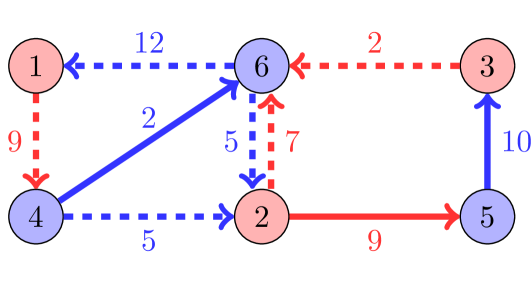
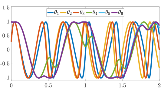
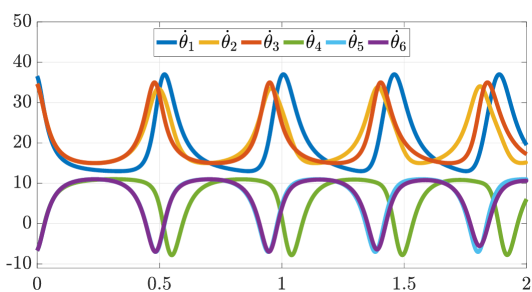
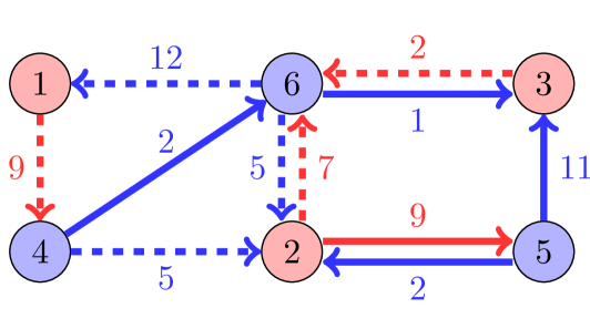
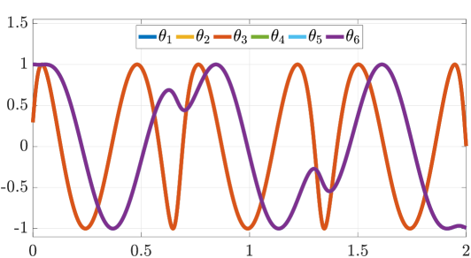
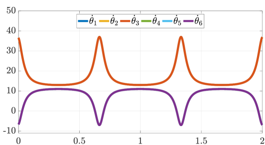
Figure 3: Fig. (a) shows the network in Example 2, where the dashed (resp. solid) edges correspond to the zero (resp. unit) entries of $H$. The partition $\mathcal{P}=\{\mathcal{P}_{1},\mathcal{P}_{2}\}$, with $\mathcal{P}_{1}=\{1,2,3\}$ and $\mathcal{P}_{2}=\{4,5,6\}$, is not synchronizable because, for instance, the sum of the weights of the incoming edges to nodes $1$ and $2$ is different (see Theorem III.1). Fig. (b) and (c) show the phases and frequencies of the oscillators as a function of time. Fig. (d) shows the modified network obtained from Theorem IV.1, which satisfies condition (i) in Theorem III.1 and leads to a synchronizable partition $\mathcal{P}$. When the natural frequencies are selected to satisfy condition (ii) in Theorem III.1, the oscillators’ phases and frequencies are synchronized as illustrated in Fig. (e) and (f).

Theorem IV.1 characterizes the smallest (measured by the Frobenius norm) structured network perturbation that ensures synchronization of a given partition. Without constraints, the optimal perturbation has a straightforward expression.

Corollary IV.2

(Unconstrained minimization problem) Let $\mathcal{H}=\{M\;:\;m_{ij}\neq 0\text{ for all }i\text{ and }j\}$. The minimization problem (3) is always feasible, and its solution is

$$\Delta^{*}=-\bar{V}_{\mathcal{P}}\bar{V}_{\mathcal{P}}^{\mathsf{T}}\bar{A}V_{\mathcal{P}}V_{\mathcal{P}}^{\mathsf{T}}.$$

Proof:

Because $h_{ij}=1$ for all $i$ and $j$, the optimality condition (6b) becomes

$$\Delta+\bar{V}_{\mathcal{P}}\Lambda V_{\mathcal{P}}^{\mathsf{T}}=0.$$

We now pre- and post-multiply both sides of the above equality by $\bar{V}_{\mathcal{P}}^{\mathsf{T}}$ and $V_{\mathcal{P}}$, respectively, and obtain

$$\Lambda =\bar{V}_{\mathcal{P}}^{\mathsf{T}}\bar{A}V_{\mathcal{P}},\;\Delta^{*}=-\bar{V}_{\mathcal{P}}\bar{V}_{\mathcal{P}}^{\mathsf{T}}\bar{A}V_{\mathcal{P}}V_{\mathcal{P}}^{\mathsf{T}},$$

where we have used (6a), $V_{\mathcal{P}}^{\mathsf{T}}V_{\mathcal{P}}=I$, and $\bar{V}_{\mathcal{P}}^{\mathsf{T}}\bar{V}_{\mathcal{P}}=I$. ∎

We now present an example where we modify the network weights to ensure synchronization of a desired partition.

Example 2

(Enforcing synchronization of a partition) Consider the network in Fig. 3(a). The dashed edges and the solid edges represent constrained and uncostrained edges, respectively. The corresponding matrices $\bar{A}$ and $H$ read as

$$\bar{A}=\begin{bmatrix}0&0&0&0&0&12\\ 0&0&0&5&0&5\\ 0&0&0&0&10&0\\ 9&0&0&0&0&0\\ 0&9&0&0&0&0\\ 0&7&2&0&0&0\end{bmatrix},H=\begin{bmatrix}0&1&1&0&0&0\\ 1&0&1&0&1&0\\ 1&1&0&0&1&1\\ 0&1&1&0&1&1\\ 1&1&1&1&0&1\\ 1&0&0&1&1&0\end{bmatrix}.$$

Notice that $H$ allows only a subset of interconnections to be modified, specifically, those corresponding to its unit entries.

It can be shown that, because condition (i) in Theorem III.1 is not satisfied (equivalently $\bar{V}_{\mathcal{P}}^{\mathsf{T}}\bar{A}V_{\mathcal{P}}\neq 0$), the network is not phase synchronizable (see Fig. 3(b) and 3(c) for an evolution of the oscillators’ phases and frequencies). From Theorem IV.1 we obtain the optimal perturbation that ensures synchronization, which leads to the network in Fig. 3(d). Notice that the network in Fig. 3(d) satisfies condition (i) in Theorem III.1. In fact, when the natural frequencies are equal within each cluster (condition (ii) in Theorem III.1), the clusters evolve cohesively; see Fig. 3(e) and 3(f). $\square$

V Conclusion

In this work we study cluster synchronization in networks of Kuramoto oscillators. We derive necessary and sufficient conditions on the network interconnection weights and on the oscillators’ natural frequencies to guarantee that the phases of groups of oscillators evolve cohesively with one another, yet independently from the phases of oscillators belonging to different groups. Additionally, we develop a control mechanism to modify the edges of a network to ensure the formation of desired clusters. Our control method is optimal, as it determines the smallest perturbation (measured by the Frobenius norm) for a desired synchronization pattern that is compatible with a pre-specified set of structural constraints.

References

- [1] F. L. Lewis, H. Zhang, K. Hengster-Movric, and A. Das. Introduction to synchronization in nature and physics and cooperative control for multi-agent systems on graphs. In Cooperative Control of Multi-Agent Systems, pages 1–21. Springer, 2014.
- [2] S. H. Strogatz. From Kuramoto to Crawford: exploring the onset of synchronization in populations of coupled oscillators. Physica D: Nonlinear Phenomena, 143(1–4):1–20, 2000.
- [3] F. A. S. Ferrari, R. L. Viana, S. R. Lopes, and R. Stoop. Phase synchronization of coupled bursting neurons and the generalized Kuramoto model. Neural Networks, pages 107–118, 2015.
- [4] F. Dörfler and F. Bullo. Synchronization in complex networks of phase oscillators: A survey. Automatica, 50(6):1539–1564, 2014.
- [5] N. Takashi and A. E. Motter. Comparative analysis of existing models for power-grid synchronization. New Journal of Physics, 17(1):015012, 2015.
- [6] T. Danino, O. Mondragon-Palomino, L. Tsimring, and J. Hasty. A synchronized quorum of genetic clocks. Nature, 463(7279):326–330, Jan 2010.
- [7] J. Kim, D. Shin, S. H. Jung, P. Heslop-Harrison, and K. Cho. A design principle underlying the synchronization of oscillations in cellular systems. Journal of Cell Science, 123(4):537–543, 2010.
- [8] D. A. Paley, N. E. Leonard, R. Sepulchre, D. Grunbaum, and J. K. Parrish. Oscillator models and collective motion. IEEE Control Systems Magazine, 27(4):89–105, 2007.
- [9] A. Schnitzler and J. Gross. Normal and pathological oscillatory communication in the brain. Nature Reviews Neuroscience, 6(4):285–296, Apr 2005.
- [10] H. Constance, B. Hagai, and P. Brown. Pathological synchronization in parkinson’s disease: networks, models and treatments. Trends in Neurosciences, 30(7):357–364, 2007.
- [11] M. Banaie, Y. Sarbaz, M. Pooyan, S. Gharibzadeh, and F. Towhidkhah. Modeling huntington’s disease considering the theory of central pattern generators. In Advances in Computational Intelligence, pages 11–19. Springer, 2009.
- [12] K. Lehnertz, S. Bialonski, M. T. Horstmann, D. Krug, A. Rothkegel, M. Staniek, and T. Wagner. Synchronization phenomena in human epileptic brain networks. Journal of Neuroscience Methods, 183(1):42–48, 2009.
- [13] Y. Kuramoto. Self-entrainment of a population of coupled non-linear oscillators. In International symposium on mathematical problems in theoretical physics, pages 420–422, Berlin, Heidelberg, 1975.
- [14] J. Gómez-Gardeñes, Y. Moreno, and A. Arenas. Synchronizability determined by coupling strengths and topology on complex networks. Physical Review E, 75:066106, Jun 2007.
- [15] Z. Zhang, A. Sarlette, and Z. Ling. Synchronization of Kuramoto oscillators with non-identical natural frequencies: a quantum dynamical decoupling approach. In IEEE Conf. on Decision and Control, pages 4585–4590, December 2014.
- [16] L. M. Pecora, F. Sorrentino, A. M. Hagerstrom, T. E. Murphy, and R. Roy. Cluster synchronization and isolated desynchronization in complex networks with symmetries. Nature communications, 5, 2014.
- [17] F. Sorrentino, L. M. Pecora, A. M. Hagerstrom, T. E. Murphy, and R. Roy. Complete characterization of the stability of cluster synchronization in complex dynamical networks. Science Advances, 2(4), 2016.
- [18] W. Lu, B. Liu, and T. Chen. Cluster synchronization in networks of coupled nonidentical dynamical systems. Chaos: An Interdisciplinary Journal of Nonlinear Science, 20(1):013120, 2010.
- [19] T. Dahms, J. Lehnert, and E. Schöll. Cluster and group synchronization in delay-coupled networks. Physical Review E, 86:016202, Jul 2012.
- [20] C. Favaretto, D. S. Bassett, A. Cenedese, and F. Pasqualetti. Bode meets kuramoto: Synchronized clusters in oscillatory networks. In IEEE American Control Conference, pages 2799–2804, Seattle, WA, USA, May 2017.
- [21] C. Favaretto, A. Cenedese, and F. Pasqualetti. Cluster synchronization in networks of kuramoto oscillators. In IFAC World Congress, 2017. To Appear.
- [22] M. T. Schaub, N. O’Clery, Y. N. Billeh, J. Delvenne, R. Lambiotte, and M. Barahona. Graph partitions and cluster synchronization in networks of oscillators. Chaos, 26(9):094821, 2016.
- [23] C. D. Godsil and G. F. Royle. Algebraic Graph Theory, volume 207 of Graduate Texts in Mathematics. Springer, 2001.
- [24] Y. Kuramoto. Self-entrainment of a population of coupled non-linear oscillators. In H. Araki, editor, Int. Symposium on Mathematical Problems in Theoretical Physics, volume 39 of Lecture Notes in Physics, pages 420–422. Springer, 1975.
- [25] M. Mirchev, L. Basnarkov, F. Corinto, and L. Kocarev. Cooperative phenomena in networks of oscillators with non-identical interactions and dynamics. IEEE Transactions on Circuits and Systems I, 61(3):811–819, 2014.
- [26] R. A. Horn and C. R. Johnson. Matrix Analysis. Cambridge University Press, 1985.