Topology in the 2d Heisenberg Model
under Gradient Flow

Abstract

The 2d Heisenberg model — or 2d O(3) model — is popular in condensed matter physics, and in particle physics as a toy model for QCD. Along with other analogies, it shares with 4d Yang-Mills theories, and with QCD, the property that the configurations are divided in topological sectors. In the lattice regularisation the topological charge $Q$ can still be defined such that $Q\in\mathbb{Z}$. It has generally been observed, however, that the topological susceptibility $\chi_{\rm t}=\langle Q^{2}\rangle/V$ does not scale properly in the continuum limit, i.e. that the quantity $\chi_{\rm t}\xi^{2}$ diverges for $\xi\to\infty$ (where $\xi$ is the correlation length in lattice units). Here we address the question whether or not this divergence persists after the application of the Gradient Flow.

1 The 2d O(3) model on the lattice

We consider square lattices of volume $V=L\times L$, and we refer to lattice units, i.e. the spacing between lattice sites is set to $1$. At each site $x$ there is a 3-component classical spin variable of length 1, $\vec{e}_{x}\in S^{2}$. The standard lattice action of a configuration $[\vec{e}\,]$ is given by

$$S[\vec{e}\,]=\beta\sum_{\langle xy\rangle}(1-\vec{e}_{x}\cdot\vec{e}_{y})\ ,$$ (1.1)

where the sum runs over the nearest neighbour lattice sites. We assume periodic boundary conditions and $\beta>0$. Obviously, this model is symmetric under global O(3) spin rotations.

In solid state physics this represents a model for a ferromagnet. Its rôle as a toy model for QCD is based on asymptotic freedom [1], a dynamically generated mass gap (which was computed with the Bethe ansatz [2]), and the existence of topological sectors.

2 Monte Carlo simulation

Since the action is real positive for any configuration, $S[\vec{e}\,]\geq 0$, it can be employed to define a probability

$$p[\vec{e}\,]=\frac{1}{Z}\,e^{-S[\vec{e}\,]}\ ,\quad Z=\int D\vec{e}\ e^{-S[\vec{e}\,]}\ .$$ (2.1)

It is normalised by the partition function $Z$, which is given by a functional integral over all configurations.

A Monte Carlo simulation generates a large set of random configurations with this probability distribution, which enable numerical measurements. To this end, we used the highly efficient cluster algorithm [3], both in its single-cluster and its multi-cluster version. It is far superior to local update algorithms, which suffer e.g. from a very long auto-correlation time with respect to the topological charge $Q$, in particular close to criticality.

3 Scale and parameters

As usual, the intrinsic scale of the system is given by its correlation length $\xi$. It describes the decay of the correlation function, which can be computed as the correlation between layer averages,

$$\langle\vec{s}_{x_{2}}\cdot\vec{s}_{y_{2}}\rangle\propto\cosh\left(-\frac{|x_{2}-y_{2}|-L/2}{\xi}\right)\ ,\quad\vec{s}_{x_{2}}=\frac{1}{L}\sum_{x_{1}}\vec{e}_{x}\ ,\quad x=(x_{1},x_{2})\ .$$ (3.1)

This proportionality relation holds if the size $L$ is large compared to $\xi$, and the numerator $|x_{2}-y_{2}|-L/2$ is sufficiently small. We determined $\xi$ by a fit in the interval $L/3\leq|x_{2}-y_{2}|\leq 2L/3$, as suggested in Ref. [4]. For a variety of parameters, our results for $\xi$ are consistent with values given in the literature, for instance in Refs. [4, 5, 6].

The correlation length depends essentially on the parameter $\beta$, and to some extent also on the size $L$. As we vary $L$ at fixed $\beta$, $\xi$ is asymptotically stable in large volumes, $L\gg\xi$. Generally, the finite-size effects are suppressed by the ratio $L/\xi$. Our study was performed in boxes of constant size,

$$L\simeq 6\,\xi\ ,$$ (3.2)

which suppresses the finite-size effects quite well. This required a fine-tuning of $\beta$ in each volume.

On the other hand, the lattice artifacts depend on the ratio of the correlation length and the lattice spacing. Since we are using lattice units, this ratio is simply given by $\xi$. Our values of $\beta$ and $\xi$, in the range $L=24\dots 404$, are listed in Table 1, in the appendix.

Hence we study the convergence to the continuum limit by increasing $L$, and increasing $\beta$ accordingly such that $L/\xi\simeq 6$ persists. This amounts to an amplification of $\xi$ at small finite-size effects, which are kept of the same magnitude, i.e. we perform a controlled extrapolation towards the continuum.

4 Topological charge and susceptibility

The geometric definition of the topological charge $Q$ [7] of a lattice configuration $[\vec{e}\,]$ has the virtue that it provides integer values, $Q[\vec{e}\,]\in\mathbb{Z}$ for all configurations (up to a subset of measure zero). We split each plaquette into two triangles, in an alternating order, as illustrated in Figure 1 on the left.

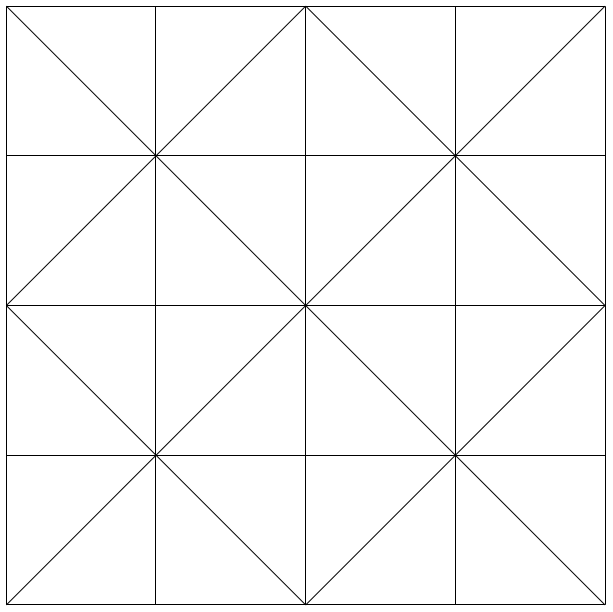
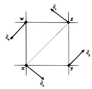
Figure 1: On the left: illustration of the division of the lattice plaquettes into triangles, in an alternating order. On the right: the spins at the vertices of each triangle — here $(\vec{e}_{x},\vec{e}_{y},\vec{e}_{z})$ and $(\vec{e}_{x},\vec{e}_{z},\vec{e}_{w})$ — span a spherical triangle, with the oriented minimal areas $A_{xyz}$ and $A_{xzw}$, respectively. Their sum defines the topological charge density at the plaquette under consideration.

The spins at the vertices of one triangle, say $(\vec{e}_{x},\vec{e}_{y},\vec{e}_{z})$, span a spherical triangle on $S^{2}$. We refer to the spherical triangle with minimal area, and a fixed orientation (which determines the sign). This oriented area $A_{xyz}$ defines the topological charge density $A_{xyz}/4\pi$, and therefore the winding number, or topological charge

$$Q[\vec{e}\,]=\frac{1}{4\pi}\sum_{\langle xyz\rangle}A_{xyz}\in\mathbb{Z}\ ,$$ (4.1)

where the sum runs over all triangles (for obtaining integer $Q$-values, it is crucial to account for the periodic boundary conditions). The explicit formulae are given in Refs. [7, 8, 9].

Parity symmetry implies $\langle Q\rangle=0$, hence the topological susceptibility takes the form

$$\chi_{\rm t}=\frac{1}{V}\left(\langle Q^{2}\rangle-\langle Q\rangle^{2}\right)=\frac{\langle Q^{2}\rangle}{V}\ .$$ (4.2)

Figure 2 shows an example for a histogram of the topological charge distribution, which tends to be approximately Gaussian.

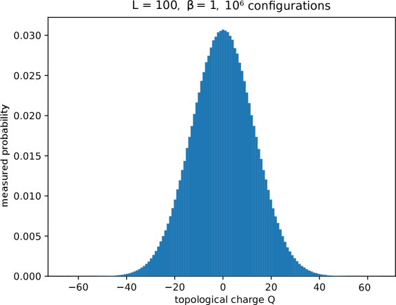
Figure 2: Histogram of the topological charges, obtained at $L=100$, $\beta=1$ with a statistics of $10^{6}$ configurations. Its shape is approximately Gaussian, with a width of $\langle Q^{2}\rangle=\chi_{\rm t}V$.

For the topological susceptibility to have a sound continuum limit, in a large volume, the (dimensionless) physical quantity $\chi_{\rm t}\xi^{2}$ should converge to a finite constant,

$$\lim_{\xi\to\infty}\ \chi_{\rm t}\xi^{2}={\rm constant}\ .$$ (4.3)

The question whether this is actually the case has been debated since the 1980s. While it was controversial for a while — based on considerations of various lattice actions and definitions of the lattice topological charge — the consensus is now that this limit diverges, i.e. the topology of this model is not well-defined in the continuum limit. This appears as a conceptual disease of the 2d O(3) model.

After the first numerical evidence for this divergence [7], a semi-classical argument was elaborated in Ref. [11]: it considers very small topological windings of a lattice configuration (“dislocations”). For increasing $\beta$ they are suppressed, but the semi-classical picture suggests that this suppression is not sufficient to compensate for the entropy growth due to the increase in $\xi$.

Later a sophisticated version of a (truncated) classically perfect lattice action was applied, which suppresses such dislocations by numerous additional couplings, beyond nearest neighbour sites [12]. However, the numerical results with this action (which were also obtained at $L\simeq 6\,\xi$) suggest that the term $\chi_{\rm t}\xi^{2}$ still does not converge to a finite value in the continuum limit. That study observed a logarithmic divergence of $\chi_{\rm t}\xi^{2}$ with $\xi$.

5 Gradient Flow

In recent years, the Gradient Flow has attracted considerable attention in the lattice community. This interest was boosted in particular by Refs. [13]. Unlike previously popular methods, where lattice configurations were smoothened ad hoc, the Gradient Flow performs such a smoothing in a controlled manner, which corresponds to a renormalisation group flow. When applied to the 2d O(3) model, one could intuitively imagine that it removes the (small) dislocations, while preserving topological winding on a large scale — in the semi-classical simplification they are represented by instantons with large radii. Hence, the question arises if the application of the Gradient Flow leads to a finite continuum limit of $\chi_{\rm t}\xi^{2}$.

The formula for the Gradient Flow in the 2d O($N$) models has been written down in Ref. [14]. Here we reproduce it for the reader’s convenience. In the continuum, the spin components $e(x)^{i},\ i=1\dots N,$ are modified according to the differential equation

$$\partial_{t}\,e(t,x)^{i}=P^{ij}(t,x)\ \Delta\,e(t,x)^{j}\ ,\quad P^{ij}(t,x)=\delta^{ij}-e(t,x)^{i}\,e(t,x)^{j}\ ,$$ (5.1)

where $t$ is the Gradient Flow time (which generically has the dimension [length]²) starting at $t=0$, and $\Delta$ is the Laplace operator. On the lattice we replace $\vec{e}(t,x)$ by the spin variable at one site, $\vec{e}(t)_{x}$, and we apply the standard discretisation of the Laplacian,

$$\Delta e(t,x)^{j}\longrightarrow e(t)_{x_{1}+1,x_{2}}^{j}+e(t)_{x_{1},x_{2}+1}^{j}+e(t)_{x_{1}-1,x_{2}}^{j}+e(t)_{x_{1},x_{2}-1}^{j}-4e(t)_{x_{1},x_{2}}^{j}\ .$$ (5.2)

For the corresponding spin rotations we apply the Runge-Kutta 4-point method. In practice we proceed as follows: for a given configuration, the gradients are computed for all spin variables, at the flow time instants which are needed for the Runge-Kutta scheme. This is done in a fixed configuration; then all the spins are simultaneously modified with a Gradient Flow time step of $dt=10^{-4}$. (After each step, the normalisation of the modified spins is re-adjusted.)

This value of $dt$ seems to be sufficiently small to avoid significant artifacts due to the flow time discretisation, whereas some discretisation effects were observed at $dt=10^{-3}$. On the other hand, for $dt=10^{-4}$ we did not find any significant difference when we modified the spins one by one lexicographically.

In order to explore the effect of the Gradient Flow on the topology towards the continuum limit, we have to set a scale for the flow time. Thus the results at various $L$ and $\beta$ can be related. We follow the recipe of Refs. [13] by considering the energy density. In our case, it is calculated as

$$E_{x}=4-\vec{e}_{x}\cdot(\vec{e}_{x_{1}+1,x_{2}}+\vec{e}_{x_{1},x_{2}+1}+\vec{e}_{x_{1}-1,x_{2}}+\vec{e}_{x_{1},x_{2}-1})$$ (5.3)

at some lattice site $x$ (it vanishes for a uniform configuration, and grows the more the spin directions differ). Its expectation value is trivially related to the mean value of the action density, $\langle E\rangle=\langle S\rangle/(\beta V)$. In QCD, Lüscher suggested to choose the Gradient Flow time unit $t_{0}$ such that $\langle E\rangle\,t_{0}^{2}=0.3$ [13]. In a 2d theory the corresponding dimensionless product reads $\langle E\rangle\,t$, and we had to fix a lower reference value, which we chose as

$$\langle E\rangle\,t_{0}=0.08\ .$$ (5.4)

As the flow time proceeds, the term $\langle E\rangle\,t$ rises from 0 to some maximum before gradually decreasing again. If the reference value is taken too large, it is not even attained for all parameter sets in our study (if one increases $L$ and $\beta$ more and more, this maximum decreases monotonously). The above reference value of $0.08$ captures lattice sizes up to $L=606$ [15], where $\beta$ is always tuned such that relation (3.2) holds.

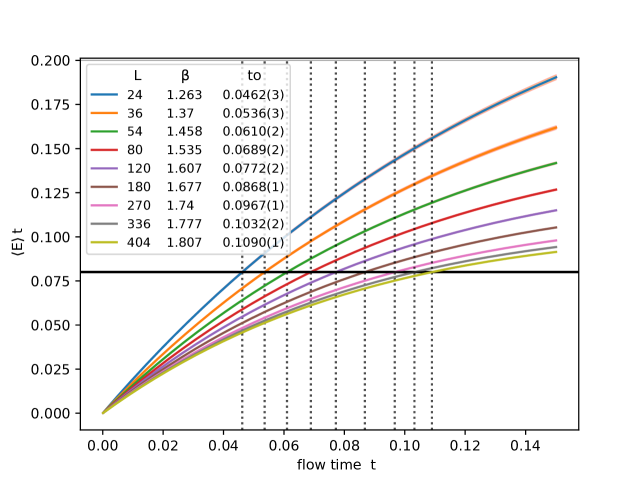
Figure 3: The Gradient Flow time evolution of the dimensionless term $\langle E\rangle\,t$, for a variety of lattice sizes $L=24\dots 404$, always with $\xi\simeq L/6$. We illustrate in particular the time $t_{0}$, where the reference value of $0.08$ is attained for the first time, so it matches the condition (5.4).

Figure 3 shows the evolution of the term $\langle E\rangle\,t$ under Gradient Flow for a variety of volumes (with the suitable $\beta$-value), and the time $t_{0}$ where it amounts to $0.08$ for the first time (in the long-time evolution it decreases again down to this value and below). The resulting $t_{0}$-values are given in the plot of Figure 3 and in Table 1; they are rather small compared to typical values in QCD.

Next we consider the correlation function (3.1),

$$C(r)=\langle\vec{s}_{x_{2}}\cdot\vec{s}_{x_{2}+r}\rangle\ .$$ (5.5)

It coincides with the connected correlation function due to the O(3) rotation symmetry, which implies $\langle\vec{s}_{x_{2}}\rangle=\vec{0}$.

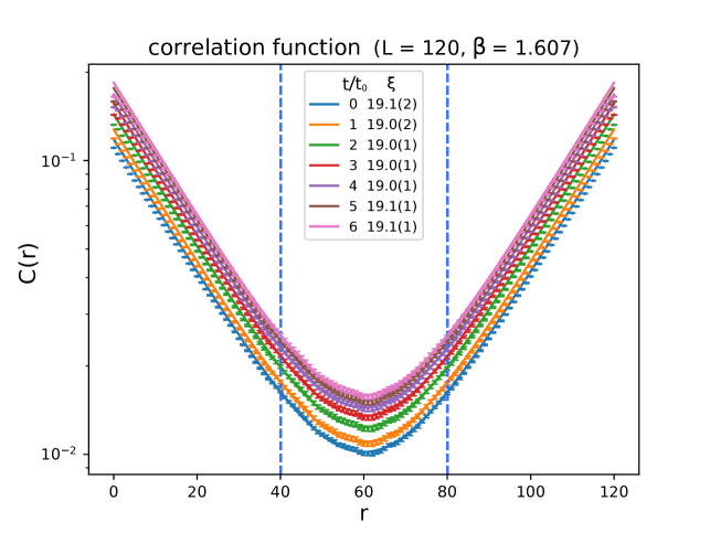
Figure 4: The correlation function $C(r)$ at $L=120$, $\beta=1.607$ (as an example). We see that the correlation at a fixed layer separation $r$ increases due to the Gradient Flow, but the correlation length $\xi$ remains almost unaltered, up to flow times as long as $6t_{0}$. This is the generic behaviour that we also observed in all other volumes under consideration. In this regime, the value of $\xi$ is a long-range property, which is hardly affected by the Gradient Flow.

Figure 4 shows an example for the behaviour of the correlation function under Gradient Flow. As the flow time $t$ proceeds, the correlation at a fixed distance $r$ is getting stronger, as one might expect. However, when we perform the fit to measure the correlation length $\xi$, according to the formula (3.1), we see that $\xi$ hardly changes. This observation holds for all parameter sets $(L,\beta)$ that we considered. Hence the intrinsic scale of the system is almost constant under the Gradient Flow, at least up to about $6\,t_{0}$, although flow times of this magnitude smoothen the configurations significantly over distances below $\xi$, as we will see in Figure 5.

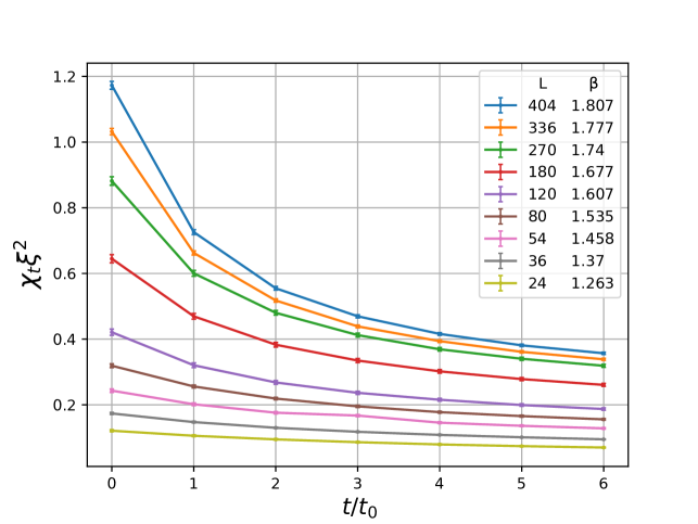
Figure 5: The evolution of the “scaling quantity” $\chi_{\rm t}\,\xi^{2}$ under the Gradient Flow, for several volumes, up to $6t_{0}$. We see that this quantity is strongly reduced by the smoothing procedure. Since $\xi$ remains almost constant, this demonstrates the destruction of a significant part of the topological windings. In this respect, the magnitude of our $t_{0}$-values is perfectly sensible.

Now we consider the quantity $\chi_{\rm t}\,\xi^{2}$, which is supposed to be the scaling term towards the continuum limit, as we mentioned before. Figure 5 shows that this term is suppressed significantly for the flow times in our study — in our three largest volumes ($L\geq 270$), $t=3t_{0}$ already reduces $\chi_{\rm t}\,\xi^{2}$ below half of its initial value. Since $\xi$ hardly changes, this reduction is due to the destruction of topological windings. This seems compatible with the picture of the elimination of dislocations. The final question is whether this effect is sufficient to entail a finite continuum limit of $\chi_{\rm t}\,\xi^{2}$, after a fixed multiple of the flow time unit $t_{0}$.

6 Continuum limit

According to Lüscher, in QCD any finite amount of Gradient Flow removes the UV divergences of the original theory [13]. This motivates us to investigate whether the same effect takes place in the 2d O(3) model, such that the Gradient Flow cures its topological UV behaviour.

Hence we finally arrive at the crucial question how $\chi_{\rm t}\,\xi^{2}$ behaves when we approach the continuum limit. This behaviour is shown in Figure 6, based on $10^{5}$ configurations in each volume, and part of the data are given in Table 1. Our study extends up to $\xi\simeq 67.7(3)$, which is close to the continuum limit indeed, but we cannot see any trend towards a convergence of $\chi_{\rm t}\,\xi^{2}$ to a finite value, at any fixed ratio $t/t_{0}=1,2\dots 6$.

At $t=0$ the data are very well compatible with a logarithmic divergence of the form $\chi_{\rm t}\,\xi^{2}=c_{1}\ln(c_{2}\xi+c_{3})$ (where $c_{i}$ are constants), as it was observed before for a classically perfect action [12], and for two types of topological lattice actions [8]. After application of the Gradient Flow, the quality of the fits to this function decreases somewhat. Figure 7 shows the data along with the logarithmic fits at flow time $t=0,\,2t_{0},\,4t_{0}$ and $6t_{0}$. For comparison, we considered another 3-parameter fit to a power-law of the form $\chi_{\rm t}\,\xi^{2}=c_{1}\xi^{c_{2}}+c_{3}$. At $t=0$ it is excellent too, but after the Gradient Flow it is a little worse than the logarithmic fits. Table 2 displays the $\chi^{2}/{\rm d.o.f}$-values for both fitting functions. In particular, at $t=0$ a power-law cannot be ruled out by the present data, although a logarithmic divergence is expected. We hope for the extension of this study to even larger volumes [15] to be helpful also in this regard.

Figure 6: The “scaling quantity” $\chi_{\rm t}\,\xi^{2}$, at flow times $t/t_{0}=0\dots 6$, and correlation length $\xi\simeq 4\dots 67.3$ (at $L/\xi\simeq 6$). Thus our study advances up to very fine lattices, but $\chi_{\rm t}\,\xi^{2}$ still does not seem to scale towards a finite continuum limit at fixed $t/t_{0}$.

7 Conclusions

The outcome of our study is illustrated in Figure 6, and the most important data are given in Table 1. After applying the Gradient Flow, with a fixed ratio $t/t_{0}$ (where $t_{0}$ has be determined according to eq. (5.4)), the quantity $\chi_{\rm t}\,\xi^{2}$ is reduced, which reveals the destruction of a significant part of the topological windings. However, as $\xi$ increases, $\chi_{\rm t}\,\xi^{2}$ still does not show any trend of a convergence towards a finite continuum value. Instead our data suggest a divergence in the continuum limit, as it was observed previously without Gradient Flow for the standard lattice action [7], a classically perfect action [12], and for topological lattice actions [8].

We add that prominent gauge theories with topological sectors, in particular SU($N$) Yang-Mills theories ($N\geq 2$) and QCD, suffer — by default — from the same problem: if we write the lattice topological susceptibility as $\chi_{\rm t}=\sum_{x}\langle q_{0}q_{x}\rangle$ (where $q$ is the topological charge density, in a conventional formulation), one encounters a divergence, due to the point $x=0$. However, in those models the problem is overcome by the application of the Gradient Flow [13].

In contrast, at this point we conclude that the topology of the 2d O(3) model seems to be ill-defined in the continuum limit, even after the application of the Gradient Flow. However, this study is going to be extended to even larger $L$ and $\xi$, in order to further check this conclusion [15].

Our interest in the issue of this article originates from a remark by Martin Lüscher. We thank him, as well as the LOC of the XXXI Reunión Anual de la División de Partículas y Campos de la Sociedad Mexicana de Física, where this talk was presented by IOS. This work was supported by DGAPA-UNAM, grant IN107915, and by the Consejo Nacional de Ciencia y Tecnología (CONACYT) through project CB-2013/222812. The computations were performed on the cluster of ICN/UNAM; we thank Luciano Díaz and Eduardo Murrieta for technical assistance.

Appendix A Numerical data and quality of the fits

Table 1 displays the most relevant numerical results in the lattice volumes under consideration, for the quantities $t_{0}$, $\xi$ and $\chi_{\rm t}$. Next we refer to our $\chi_{\rm t}\,\xi^{2}$-values as a function of $\xi$, shown in Figure 6. Figure 7 illustrates the logarithmic fits to the data at flow time $t=0,\,2t_{0},\,4t_{0}$ and $6t_{0}$. Finally, Table 2 gives the quality of the fits to a logarithmic and a power-law function, as described in the last paragraph of Section 6.

$L$	$\beta$	$t_{0}$	$\xi$		$\chi_{\rm t}$  (in units of $10^{-3})$
			$t=0$	$6\,t_{0}$	$t=0$	$t_{0}$	$3\,t_{0}$	$6\,t_{0}$
24	1.263	0.0462(3)	4.01(5)	4.00(4)	7.51(4)	6.58(4)	5.38(3)	4.38(2)
36	1.37	0.0536(3)	6.05(5)	6.04(3)	4.74(3)	4.03(2)	3.22(2)	2.60(1)
54	1.458	0.0610(2)	9.0(1)	9.10(7)	2.99(2)	2.47(1)	2.04(1)	1.550(9)
80	1.535	0.0689(2)	13.1(1)	13.1(1)	1.86(1)	1.495(8)	1.139(6)	0.907(5)
120	1.607	0.0772(2)	19.1(2)	19.1(2)	1.154(5)	0.879(4)	0.649(3)	0.513(2)
180	1.677	0.0868(1)	30.6(3)	30.6(3)	0.691(3)	0.503(2)	0.358(2)	0.278(1)
270	1.74	0.0967(1)	45.6(3)	45.6(3)	0.424(2)	0.289(1)	0.1983(9)	0.1534(7)
336	1.777	0.1032(2)	56.4(2)	56.3(2)	0.324(1)	0.2084(9)	0.1381(6)	0.1066(5)
404	1.807	0.1090(1)	67.7(3)	67.7(3)	0.256(1)	0.1585(7)	0.1024(5)	0.0779(4)

Table 1: A summary of our numerical results in the nine volumes $V=L\times L$ that we investigated. In each volume, $\beta$ was tuned such that $L/\xi\simeq 6$, and $t_{0}$ was determined by the condition $\langle E\rangle\,t_{0}=0.08$. We see that the correlation length $\xi$ hardly changes under Gradient Flow, but the topological susceptibility is significantly reduced as we proceed up to $6t_{0}$. These results are based on a statistics of $10^{5}$ configurations in each volume.

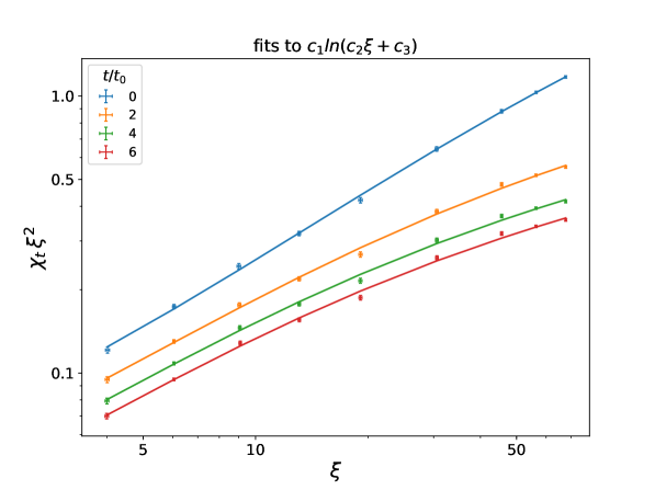
Figure 7: The fits of our data in Figure 6, at various Gradient Flow times, to the logarithmic ansatz $\chi_{\rm t}\,\xi^{2}=c_{1}\ln(c_{2}\xi+c_{3})$ (where $c_{i}$ are constants). These fits work well, and they suggest the divergence of $\chi_{\rm t}\,\xi^{2}$ in the continuum limit.

fitting function	$t=0$	$t_{0}$	$2t_{0}$	$3t_{0}$	$4t_{0}$	$5t_{0}$	$6t_{0}$
$c_{1}\,\ln(c_{2}\,\xi+c_{3})$	1.07	1.34	1.63	2.20	1.82	1.89	1.91
$c_{1}\,\xi^{c_{2}}+c_{3}$	1.01	1.58	1.94	2.32	2.12	2.16	2.18

Table 2: The $\chi^{2}/{\rm d.o.f}$-values for two fits of our $\chi_{\rm t}\,\xi^{2}$-results as a function of $\xi$. We consider two 3-parameter fitting functions, with a logarithmic and a power-law divergence in the continuum limit. At Gradient Flow time $t=0$ both fits are excellent, but in the range $t=t_{0}\dots 6t_{0}$ they become somewhat worse, in particular for the power-law.

References

References

- [1] Polyakov A M 1975 Phys. Lett. B 59 79
- [2] Hasenfratz P, Maggiore M and Niedermayer F 1990 Phys. Lett. B 245 522
- [3] Wolff U 1989 Phys. Rev. Lett. 62 361
- [4] Wolff U 1990 Nucl. Phys. B 334 581
- [5] Apostolakis J, Baillie C F and Fox G C 1991 Phys. Rev. D 43 2687
- [6] J-K Kim 1994 Phys. Rev. D 50 4663
- [7] Berg B and Lüscher M 1981 Nucl. Phys. B 190 412
- [8] Bietenholz W, Gerber U, Pepe M and Wiese U-J 2010 JHEP 1012 020
- [9] Bautista I et al. 2015 Phys. Rev. D 92 114510
- [10] Bietenholz W, Cichy K, de Forcrand P, Dromard A and Gerber U 2016 PoS LATTICE2016 321
- [11] Lüscher M 1982 Nucl. Phys. B 200 61
- [12] Blatter M, Burkhalter R, Hasenfratz P and Niedermayer F 1996 Phys. Rev. D 53 923
- [13] Lüscher M 2010 JHEP 1008 071, PoS LATTICE2010 015
- [14] Makino H and Suzuki H 2015 PTEP 2015 033B08
- [15] Bietenholz W, de Forcrand P, Gerber U, Mejía-Díaz H and Sandoval I O, in preparation
- [16] Giusti L, Rossi G C and Testa M 2004 Phys. Lett. B 587 157 Lüscher M 2004 Phys. Lett. B 593 296 Giusti L and Lüscher M 2009 JHEP 0903 013 Lüscher M and Palombi F 2010 JHEP 1009 110