Improving spliced alignment for identification of ortholog groups and multiple CDS alignment

Abstract

The Spliced Alignment Problem (SAP) that consists in finding an optimal semi-global alignment of a spliced RNA sequence on an unspliced genomic sequence has been largely considered for the prediction and the annotation of gene structures in genomes. Here, we re-visit it for the purpose of identifying CDS ortholog groups within a set of CDS from homologous genes and for computing multiple CDS alignments. We introduce a new constrained version of the spliced alignment problem together with an algorithm that exploits full information on the exon-intron structure of the input RNA and gene sequences in order to compute high-coverage accurate alignments. We show how pairwise spliced alignments between the CDS and the gene sequences of a gene family can be directly used in order to clusterize the set of CDS of the gene family into a set of ortholog groups. We also introduce an extension of the spliced alignment problem called Multiple Spliced Alignment Problem (MSAP) that consists in aligning simultaneously several RNA sequences on several genes from the same gene family. We develop a heuristic algorithmic solution for the problem. We show how to exploit multiple spliced alignments for the clustering of homologous CDS into ortholog and close paralog groups, and for the construction of multiple CDS alignments. An implementation of the method in Python is available on demande to SFA@USherbrooke.ca.

1 Introduction

Spliced alignment consists in aligning spliced gene products against unspliced DNA sequences [8]. It is a key step for genome annotation, gene prediction, identification of gene structures and alternative splicing studies [7, 17]. The quality of the transcriptome annotation is greatly improved with the use of spliced RNA data of related genes or genomes. In the past two decades, several spliced alignment tools have been developed for aligning RNA or protein data on genomic DNA ([9, 16] for example). Such methods look for an alignment that maximizes the sequence similarity and splice site consensus signals between a short RNA sequence and a large genome sequence. They are specifically developed for genome annotation purpose, without any assumption on the homology of the compared sequences. So, in order to achieve high sensitivity, they look for high-identity alignments in order to avoid as much false positive alignments as possible. As a consequence, these methods perform accurately for the comparison of sequences from closely related genomes but often misses the alignment of homologous sequences from distant genomes.

Although spliced alignment methods are classically used for the prediction and annotation of genes in genomes, they can also be specifically designed for the purpose of aligning sequences from a priori homologous genes. In this context, they can be used as a preliminary step for the identification of orthologous transcripts or proteins isoforms [17], the transfer of transcript annotations between homologous genes [1] or for studying the evolution of RNA isoforms in a gene family [4, 10, 12]. Spliced alignment can also improve the accuracy of multiple homologous CDS alignment by making use of one or several reference genes. Current spliced alignment methods make use of the gene structure by accounting for possible splice sites predicted in the gene sequence. However, accounting for the exact exon-intron structure of the gene, when it is known, can help improve the alignment further. Moreover, current methods do not make use of the exon structure of the query RNA sequence because they were mainly designed for aligning EST and RNA-seq data, for which the exon structure is unknown, on genomic sequences. However, when the RNA sequence is given with its corresponding gene sequence, it is possible to easily recover its exon structure and use this information for the spliced alignment against an other gene.

In this paper, we are interested in the Spliced Alignment Problem (SAP) that consists in finding an optimal spliced alignment between a CDS and a gene that captures all sequence similarities including those between phylogenetically distant homologous sequences. For aligning a CDS against a gene, under the assumption of homology between the sequences, it is possible to make use of the splicing structure of the sequences in order to accurately detect sequence homologies even in the case of phylogenetically distant sequences. First, in Section 3, we introduce a constrained version of the SAP problem and we present a CDS-gene spliced alignment method that exploits full information on the structure of the input CDS and the input gene in order to compute high-coverage accurate alignments. Second, in Section 4, we show how this method can be directly used for clustering the set of CDS of a gene family into ortholog and close paralog groups, allowing one-to-one as well as one-to-many orthology relations. Third, in Section 5, we introduce an extension of the Spliced Alignment Problem called Multiple Spliced Alignment Problem (MSAP) that consists in finding an optimal multiple spliced alignment between a set of CDS and a set of genes. The MSAP problem also extends a homonym problem introduced in [8] for the simultaneous spliced alignment of a set of CDS on a single gene. We describe an algorithm for the MSAP problem that consists in combining pairwise spliced alignments into a multiple spliced alignment, by merging progressively the pairwise alignments while filtering out false-positive sub-alignments. We show that the multiple spliced alignments allow to identify homologous segments (exons) across a set of homologous genes and to compute accurate CDS ortholog groups and multiple CDS alignments. Finally, Section 6 is devoted to the evaluation of our method by comparing it to other methods based on the application to the analysis of set of homologous CDS and genes from the Ensembl-Compara database.

2 Preliminaries: genes, CDS, splicing and orthology

In this section, we give some formal definitions that will be useful for the remaining of the paper. Given a set $S$, $|S|$ denotes the size of $S$, and given a sequence or an interval $T$, $\texttt{length}(T)$ denotes the length of $T$.

Gene, Exon and CDS: A gene is DNA sequence on the alphabet of nucleotides $\Sigma=\{A,C,G,T\}$. Given a gene $G$ of length $n$, an exon of $G$ is a pair of integers $(a,b)$ such that $1\leq a\leq b\leq n$. The sequence of an exon $(a,b)$ of $G$, denoted by $G[a,b]$, is the segment of $G$ identified by its start and end positions $a$ and $b$ in $G$. A CDS $C$ of $G$ is a chain of exons of $G$, $C=\{(a_{1},b_{1}),\ldots,(a_{j},b_{j})\}$ such that for any two successive exons $(a_{i},b_{i})$ and $(a_{i+1},b_{i+1})$ in $C$, $b_{i}<a_{i+1}$. Thus, the exons of $C$ are non-overlapping and totally ordered by increasing location on the gene. We denote by $C[i]$ the i^th element of $C$. We denote the set of introns induced by $C$ by $\texttt{Intron}(C)=\{(b_{i},a_{i+1})~{}|~{}1\leq i<j\}$. We denote by $\mathcal{C}(G)$ the set of existing CDS of a gene $G$ and by $\mathcal{E}(G)$ the set of gene exons of $G$ composing these CDS, $\mathcal{E}(G)=\bigcup_{C\in\mathcal{C}(G)}{C}$. For example, if $|G|=100$ and $\mathcal{C}(G)$ contains two CDS $C_{1}=\{(11,20),(31,50)\}$ and $C_{2}=\{(11,25),(31,50),(61,90)\}$, then $\mathcal{E}(G)=\{(11,20),(11,25),(31,50),(61,90)\}$.

The sequence of a CDS $C$ of $G$, denoted by $G_{C}$, is the concatenation of the sequences of gene exons composing $C$ in the order in which they appear in $C$. So, the length of the CDS sequence $G_{C}$ equals the sum of the length of the gene exon sequences composing $G_{C}$. By extension of the definition of a gene exon, an exon of a CDS sequence $G_{C}$ of length $m$ is a pair of integers $(k,l)$ such that $1\leq k\leq l\leq m$ and the segment $G_{C}[k,l]$ of $G_{C}$, identified by its start and end positions $k$ and $l$ in $G_{C}$, is exactly one of the gene exon sequences composing $G_{C}$. We denote by $\mathcal{E}(G_{C})$ the set of CDS exons composing a CDS sequence $G_{C}$. Note that $|\mathcal{E}(G_{C})|=|C|$. For the example of gene $G$ with a CDS $C_{1}$ given above, $|G_{C_{1}}|=30$ and $\mathcal{E}(G_{C_{1}})=\{(1,10),(11,30)\}$.

Gene family, orthology relationships: A gene family $\mathcal{G}$ is a set of homologous genes that have derived from the same original gene by duplication and speciation events. The genes of a gene family are supposed to have similar segments and biochemical functions. The evolution of a gene family is represented by a rooted binary tree $T$ whose set of leaves is $\mathcal{G}$ and internal nodes are ancestral genes that precede an ancestral event labeled as duplications or speciations. A node is an ancestor of a gene (leaf) if it is on the path between this leaf and the root of the tree. The lowest common ancestor (LCA) of two genes is the common ancestor to both genes that is the most distant from the root. The orthology relationship between genes can be defined from two different points of view. From a gene tree point of view, two genes of $\mathcal{G}$ are called orthologs if their lowest common ancestor in the tree $T$ is a speciation, otherwise they are called paralogs. From a similarity point of view, orthologous genes have similar sequences, structures and functions. For instance, reciprocal best hits are a common approach for the definition of orthology relations in comparative genomics.

Splicing and spliced alignment: In molecular biology, a eukaryotic mature RNA sequence is obtained from a RNA transcript by a phenomenon called splicing that consists in removing the sequences between any two successive exons of a CDS called introns and joining the resulting exon extremities. The CDS is the segment of the mature RNA sequence that is translated into a protein sequence. In practice, a full CDS sequence has a length that is multiple of $3$ and it starts with a codon "ATG" and ends with a codon "TAA", "TAG" or "TGA".

A spliced alignment is an alignment between a CDS and a gene sequence that allows to identify conserved exons sequences. See Figure 1 for example. Formally, a spliced alignment of a CDS sequence $G_{C}$ of length $m$ on a gene $H$ of length $n$ is a chain of quadruplets $A=\{(k_{1},l_{1},a_{1},b_{1}),\ldots,(k_{j},l_{j},a_{j},b_{j})\}$ called blocks such that for any block $(k,l,a,b)$ of $A$, $1\leq k\leq l\leq m$, $a=b=0$ or $1\leq a\leq b\leq n$, and for any two successive blocks $(k_{i},l_{i},a_{i},b_{i})$ and $(k_{i+1},l_{i+1},a_{i+1},b_{i+1})$, $l_{i}=k_{i+1}-1$. Moreover, for any two blocks $A[i_{1}]$ and $A[i_{2}]$ with $i_{1}<i_{2}$, we have $b_{i_{1}}<a_{i_{2}}$ if $a_{i_{2}}\neq 0$.

The blocks $(k,l,a,b)$ of $A$ such that $1\leq a\leq b\leq n$ correspond to conserved exon segments $G_{C}[k,l]$ and $H[a,b]$ between the CDS and the gene sequence. We call them conserved blocks and we denote the set of conserved blocks of $A$ by $\texttt{Cons}(A)=\{(k_{i},l_{i},a_{i},b_{i})\in A~{}|~{}b_{i}\neq 0\}$. The blocks $(k,l,a,b)$ such that $a=b=0$ correspond to exon segments $G_{C}[k,l]$ in the CDS sequence that are absent in the gene sequence. We call them deleted blocks. In other terms, the blocks composing $A$ correspond to a chain of non-overlapping segments of the CDS sequence $G_{C}$ that are increasingly located on $G_{C}$ and cover entirely $G_{C}$. Moreover the conserved blocks correspond to a chain of non-overlapping segments of the gene sequence $H$ that are also increasingly located on $H$. Thus, there is no crossing in the alignment. We denote by $A[i]$ the i^th block of $A$.

The spliced alignment $A$ also induces a set of putative gene intron segments. These intron segments are the gene segments that lie between two successive blocks of $A$ that are both conserved in the gene sequence. We denote the set of introns induced by the alignment $A=\{(k_{1},l_{1},a_{1},b_{1}),\ldots,(k_{j},l_{j},a_{j},b_{j})\}$ by $\texttt{Intron}(A)=\{(b_{i},a_{i+1})~{}|~{}1\leq i<j~{}\texttt{and}~{}b_{i}\neq 0~{}\texttt{and}~{}b_{i+1}\neq 0\}$. Note that if all blocks composing $A$ are conserved, then $|\texttt{Intron}(A)|=|A|-1$.

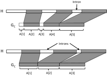
Figure 1: Top. A spliced alignment between a CDS sequence $G_{C}$ and a gene $H$ composed of $5$ blocks, $3$ conserved blocks ($A[2]$, $A[4]$ and $A[5]$) and $2$ deleted blocks ($A[1]$ and $A[3]$), that induce $1$ putative intron. Bottom. A spliced alignment composed of $3$ conserved blocks that induce $2$ putative introns.

3 Computation of spliced alignment

In this section, we first re-call two well-known versions of the spliced alignment problem and we introduce a third version that we study in this paper. Next, we describe a heuristic algorithm for the last problem.

Spliced alignment problems: Given a gene sequence $H$, $H[0,0]$ corresponds to the empty sequence. Given two nucleotide sequences $S_{1}$ and $S_{2}$, let $\texttt{sim}(S_{1},S_{2})$ denote the score of an optimal global alignment between them. The following is a reformulation of the less constrained version of the spliced alignment problem studied in [9]. This formulation allows a unified framework to compare the problem with some more constrained versions of the problem formulated thereafter.

Spliced Alignment Problem I (SAP_I):
Input: A CDS sequence $G_{C}$ from a gene $G$ ; a gene sequence $H$.
Output: A spliced alignment $A$ of $G_{C}$ on $H$ that maximizes

$$\sum_{(k,l,a,b)\in A}{\texttt{sim}(G_{C}[k,l],H[a,b])}$$

The (SAP_I) problem only accounts for the alignment scores between the segments composing the blocks of the spliced alignment. In practice, in more than 99$\%$ of real cases of splicing, the removed intron sequences start with a dinucleotide sequence "GT" and ends with a dinucleotide sequence "AG" respectively called canonical donor and acceptor splice sites [3, 15]. Thus, in order to improve the accuracy of the spliced alignment, a more constrained version of the problem allows to account for the intron segments induced by an alignment. Given a nucleotide sequence $S$, let $\texttt{intr}(S)$ denote the intron score of $S$ accounting for the presence or absence of canonical splice sites at the extremities of $S$. A sequence with two canonical splice sites at its extremity has a higher score than a sequence with only one which has a higher score than a sequence without canonical splice sites. A more constrained version of the spliced alignment problem studied in [9] is the following.

Spliced Alignment Problem II (SAP_II):
Input: A CDS sequence $G_{C}$ from a gene $G$ ; a gene sequence $H$.
Output: A spliced alignment $A$ of $G_{C}$ on $H$ that maximizes

$$\sum_{(k,l,a,b)\in A}{\texttt{sim}(G_{C}[k,l],H[a,b])}+\sum_{(b,a)\in\texttt{Intron}(A)}{\texttt{intr}(H[b,a])}$$

The SAP_I and SAP_II problems do not account for the exon structure of the CDS sequence and the exon-intron structure of the gene sequence. In order to further improve the accuracy of the spliced alignment, we consider a more constrained version of the problem that accounts for the actual exons in the CDS and the gene sequence. Given a conserved block $(k,l,a,b)$ of a spliced alignment, let $\texttt{exon}_{\mathcal{E}(G_{C}),\mathcal{E}(H)}(k,l,a,b)$ denote the score of a conserved block accounting for the correspondence of the block with an actual exon in the CDS or in the gene sequence. A block that corresponds to an exon in both sequences has a higher score than a block with an exon correspondence in only one of the sequences which has a higher score than a block without any exon correspondence. The more constrained version of the problem is defined as follows.

Spliced alignment Problem III (SAP_III):
Input: A CDS sequence $G_{C}$ from a gene $G$ ; the set of exons $\mathcal{E}(G_{C})$ of $G_{C}$ ; a gene sequence $H$ ; the set of exons $\mathcal{E}(H)$ of $H$.
Output: A spliced alignment $A$ of $G_{C}$ on $H$ that maximizes

$$\sum_{(k,l,a,b)\in A}{\texttt{sim}(G_{C}[k,l],H[a,b])}+\sum_{(k,l,a,b)\in\texttt{Cons}(A)}{\texttt{exon}_{\mathcal{E}(G_{C}),\mathcal{E}(H)}(k,l,a,b)}$$

$$+\sum_{(b,a)\in\texttt{Intron}(A)}{\texttt{intr}(H[b,a])}$$

Heuristic algorithm for the (SAP_III) problem: The general approach followed by most heuristic spliced alignment methods for the SAP_I and SAP_II problems consists in first computing high-identity local alignments between the CDS and the gene sequence. In a second step, these local alignments are used as anchors and a global alignment algorithm is applied in the regions between the anchor alignments in order to complete the spliced alignment. Our heuristic spliced alignment method for the SAP_III problem also starts with the computation of highly conserved local alignments used as anchors. However, in a second step, we use the exon structure of the CDS sequence to extend the anchors towards the extremities of the CDS exons containing them. This steps drastically reduces the length of the CDS sequences remaining between the extended anchor in the deleted blocks. In a third step, we apply a global alignment in the remaining regions. In a fourth step, we correct the splicing junctions in order to recover GT$/$AG canonical splice sites that were missed because of the insertion or deletion of nucleotides in the exon sequences, resulting in gaps in the block alignments. Finally, in a fifth step, we use the exon-intron structure of the gene sequence to further correct the block extremities. The details of the steps composing the method are given below.

Step 1. Local alignment. This step is achieved using Translated Blast (tblastx) with an E-value threshold of $10^{-2}$ in order to obtain local alignments. Tblastx is used in order to account for the translation of the sequences into amino acid sequences. This allows to detect amino acid sequence conservation even in the presence of translational frameshifts.

Step 2. Block extension based on CDS exons. This step is repeated iteratively in order to prioritize highly conserved local alignments. Local alignments are classified into four groups according to their E-value scores, less than $10^{-7}$, between $10^{-7}$ and $10^{-5}$, between $10^{-5}$ and $10^{-3}$ and greater than $10^{-3}$. For each group from the more to the less conservative, a maximum size set of pairwise compatible anchors is kept as conserved blocks and the blocks are extended as follows. Given a block extremity that does not correspond to a CDS exon extremity, the block extremity is extended until the closest CDS exon extremity if this extension does not decrease the percentage of nucleotide identity in the block alignment. If the extension induces an overlapping with another conserved block on the CDS sequence, the other block is trimmed in order to free space for the extension. In this case, the extension and the trimming are applied only if they strictly increases the nucleotide identity of the two block alignments. See Figure 2 for an illustration.

Step 3. Global alignment of remaining regions. This step consists in applying a classical global alignment algorithm for the regions of the CDS in deleted blocks, not yet covered by the spliced alignment. The conserved blocks induced by the global alignment are added in the spliced alignment. For each comparison, we make use of an exact semi-global alignment that penalizes no end gaps in the two compared sequences.

Step 4. Correction of exon junctions. In this step, the introns induced by the spliced alignment are refined. Given an induced intron $(b,a)$ between two conserved blocks of the alignment, if the donor and acceptor splice sites of the intron are not both canonical, we look for a shift of the block junction that corresponds to a pair of canonical splice sites and does not decrease the percentage of nucleotide identity in the flanking block alignments. The space search is limited to a maximum of 30-nucleotide shift and 3-codon gaps.

Step 5. Correction of block extremities based on gene exons. This step is composed of two phases. First, each extremity of a conserved block that does not correspond to a gene exon extremity or a CDS exon extremity is trimmed until the closest gene exon extremity if there exists such a gene exon extremity. This allows to free space in order to extend neighboring conserved block extremities in a second phase. In the second phase, each conserved block extremity that still does not correspond to a gene exon extremity or a CDS exon extremity is extended until the closest available gene exon extremity if this extension does not decrease the nucleotide identity of the block alignment. See Figure 2 for an illustration.

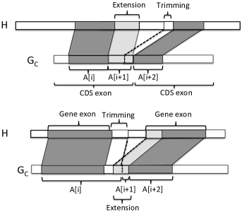
Figure 2: Top. Illustration of Step 2 of the heuristic spliced alignment method: the right extremity of the block $A[i]$ is extended according to the first CDS exon, and that requires the trimming of the left extremity of the block $A[i+2]$. Bottom. Illustration of Step 5: the right extremity of the block $A[i]$ is trimmed according to the first gene exon, and next the left extremity of the block $A[i+2]$ is extended according to the second gene exon.

Note that, the algorithm used for each step of the method can be replaced by any other algorithm solving the same problem. For instance, Step 1 can use a faster local alignment algorithm than tblastx. Steps 3 and 4 can be merged by using a global alignment algorithm that accounts simultaneously for the sequence similarities and the intron scores such as the global alignment algorithm developed [9]. The output of the spliced alignment method is a spliced alignment whose blocks extremities maximize the correspondence with the exon extremities of the input CDS and gene sequences.

4 Identification of CDS ortholog groups

In this section, we give a definition of CDS ortholog groups based on pairwise spliced alignments. We first start with a definition of orthologous CDS.

In [17], an extension of the concept of gene orthology to spliced transcript orthology was introduced. They defined orthologous transcripts as two structurally similar transcripts from two orthologous genes. In [12], we have introduced a new protein tree model of transcript evolution along gene trees, that is similar to the gene tree model of gene evolution along species tree with duplication and speciation events. In the model of transcript evolution along gene trees, we have introduced a third type of event called creation representing the separation of two lineages of structurally different transcripts. This model have led to an extended definition of protein and transcript orthology, based on the protein tree model and relaxing the constraint that two orthologous transcripts should come from orthologous genes. We call two transcripts ortholog if their LCA in the protein tree is a speciation or a duplication (not a creation), otherwise they are called paralogs. From a similarity point of view, the corresponding definition of transcript orthology is that two transcripts are orthologs if they are structurally similar and come from two homologous genes, not necessarily orthologous genes. Next, two orthologous transcripts are ortho-orthologs if they come from orthologous genes, and para-orthologs otherwise. Note, that our definition of ortho-orthologs then corresponds to the definition of orthologous transcripts from [17]. Thus, the orthology relationship between two transcripts from two homologous genes relies on the evaluation of the structural similarity between the transcripts. Here, we evaluate this structural similarity using the CDS associated to the transcripts.

CDS orthology: Let $C_{1}$ and $C_{2}$ be two CDS from two homologous genes $G$ and $H$ respectively. Let $A_{1}$ be a spliced alignment of the CDS sequence $G_{C_{1}}$ on the gene sequence $H$, and $A_{2}$ a spliced alignment of $H_{C_{2}}$ on $G$. Using $A_{1}$ and $A_{2}$, we define $C_{1}$ and $C_{2}$ as orthologs if:
(1) $|~{}C_{1}~{}|=|~{}C_{2}~{}|$ and
(2) $\texttt{Intron}(A_{1})=\texttt{Intron}(C_{2})$ or $\texttt{Intron}(A_{2})=\texttt{Intron}(C_{1})$ and
(3) for any $i,1\leq i\leq~{}|~{}C_{1}~{}|$, $[\texttt{length}(C_{1}[i])-\texttt{length}(C_{2}[i])]~{}\%~{}3=0$.

In other terms, $C_{1}$ are $C_{2}$ as orthologs if (1) they have the same number of exons, (2) the spliced alignment of $C_{1}$ on $H$ induced the same introns as $C_{2}$ in $H$ or the spliced alignment of $C_{2}$ on $G$ induces the same introns as $C_{1}$ in $G$ and (3) the lengths of each pair of corresponding exons in $C_{1}$ and $C_{2}$ should be congruent modulo $3$. The conditions (1) and (2) ensure that the two CDS have the same exon structure. The condition (3) ensures that the two CDS are translated in the same codon phase in each pair of corresponding exons.

Note that this definition only requires that one of the spliced alignments $A_{1}$ and $A_{2}$ supports the orthology relation. An alternative more stringent definition of CDS orthology consists in requiring the reciprocity, i.e. that $A_{1}$ and $A_{2}$ both support the orthology relation, by using the ’and’ statement instead of the ’or’ statement in the condition (2).

CDS ortholog groups: Given a set of CDS $\mathcal{C}$ from a set of homologous genes $\mathcal{G}$, the transitivity of the CDS orthology relation is used to identify distant orthologs and co-orthologs in $\mathcal{C}$ that cannot be identified by means of the CDS structural similarity. Such orthologs are typically missed because of partial spliced alignments due to low sequence similarity.

The CDS orthology relation on $\mathcal{C}$ is then extended into an equivalence relation such that for any three CDS $C_{1},C_{2},C_{3}$ in $\mathcal{C}$, if $C_{1}$ and $C_{2}$ are orthologs and $C_{2}$ and $C_{3}$ are orthologs, then $C_{1}$ and $C_{3}$ are also orthologs. The CDS ortholog groups are defined as the equivalence classes of the resulting equivalence relation.

5 Computation of multiple spliced alignment

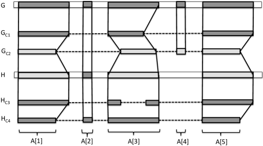
Figure 3: Illustration of a multiple spliced alignment of $4$ CDS sequences, $G_{C_{1}},G_{C_{2}}$ of a gene $G$ and $H_{C_{3}},H_{C_{4}}$ of a gene $H$ on the genes $G$ and $H$. The multiple spliced alignment is composed of $5$ blocks such that $A[1],A[3],A[5]$ have occurrences in all sequences, while $A[2]$ is conserved in $G$, $H$ and $H_{C_{4}}$ and $A[4]$ is only present in $G$ and $G_{C_{2}}$. The pairwise spliced alignment induced for the CDS sequence $G_{C_{2}}$ on the gene sequence $H$ is depicted in gray color.

The concept of spliced alignment was extended in order to define multiple spliced alignments [2, 8]. A multiple spliced alignment was then defined as a simultaneous spliced alignment of several RNA sequences on a single gene sequence. Multiple spliced alignment allows to improve the accuracy of gene structure prediction by making use of several RNA targets simultaneously. Here, we further extend the concept in order to consider the simultaneous spliced alignment of several CDS sequences on several genes. See Figure 3 in Appendix for example.

Based on the formalism introduced in Section 2, we defined a multiple spliced alignment of a set of CDS sequences $\mathcal{C}$ on a set of genes $\mathcal{G}$ as a chain $A=\{A[1],\ldots,A[j]\}$ of sets called multi-blocks such that $A[i]$ denotes the i^th multi-block of $A$. Each multi-block $A[i]$ is a set of pairs $A[i]=\{(s_{i}^{x},e_{i}^{x})~{}|~{}x\in\mathcal{C}\cup\mathcal{G}\}$ such that for any sequence $x\in\mathcal{C}\cup\mathcal{G}$, $s_{i}^{x}=e_{i}^{x}=0$ or $1\leq s_{i}^{x}\leq e_{i}^{x}\leq\texttt{length}(x)$. For any two multi-blocks $A[i_{1}]$ and $A[i_{2}]$ with $i_{1}<i_{2}$, and any sequence $x\in\mathcal{C}\cup\mathcal{G}$, $e_{i_{1}}^{x}<s_{i_{2}}^{x}$ if $s_{i_{2}}^{x}\neq 0$. Moreover, for any CDS sequence $x\in\mathcal{C}$, the set of segments of $x$ induced by $A$, $\{x[s_{i}^{x},e_{i}^{x}]~{}|~{}1\leq i\leq j~{}\texttt{and}~{}e_{i}^{x}\neq 0\}$ cover entirely $x$.

A multi-block $A[i]=\{(s_{i}^{x},e_{i}^{x})~{}|~{}x\in\mathcal{C}\cup\mathcal{G}\}$ corresponds to a group of segments (one segment $x[s_{i}^{x},e_{i}^{x}]$ for each sequence $x$ such that $e_{i}^{x}\neq 0$) that are homologs and absent in any sequence $x$ such that $e_{i}^{x}=0$. By definition, the multi-blocks composing $A$ are non-overlapping in any sequence and increasingly located on each of the sequence. Thus, there is no crossing in the alignment.

A multiple spliced alignment $A=\{A[1],\ldots,A[j]\}$ of a set of CDS sequences $\mathcal{C}$ on a set of genes $\mathcal{G}$ induces a spliced alignment $A_{x,y}$ for each pair $(x,y)\in\mathcal{C}\times\mathcal{G}$. The induced spliced alignment consists of a reduction of the multi-blocks $A[i]$, $1\leq i\leq j$ such that $e_{i}^{x}\neq 0$, i.e the multi-blocks in which the segment of the CDS sequence $x$ is not empty, $A_{x,y}=\{(s_{i}^{x},e_{i}^{x},s_{i}^{y},e_{i}^{y})~{}|~{}1\leq i\leq j~{}\texttt{and}~{}e_{i}^{x}\neq 0\}$.

Given a spliced alignment $A_{x,y}$ of a CDS sequence $x$ on a gene sequence $y$, let $\mathbb{S}(A_{x,y})$ denote the score of the spliced alignment $A_{x,y}$ as defined for the SAP_I, SAP_II or SAP_III problem. We defined the corresponding multiple spliced alignment problem as follows:

Multiple spliced alignment Problem (MSAP_$\mathbb{S}$):
Input: a set of CDS sequence $\mathcal{C}$ ; a set of genes $\mathcal{G}$.
Output: A multiple spliced alignment $A$ of $\mathcal{C}$ on $\mathcal{G}$ that maximizes the sum of the scores of induced pairwise spliced alignments: $\sum_{(x,y)\in\mathcal{C}\times\mathcal{G}}{\mathbb{S}(A_{x,y})}$.

Heuristic algorithm for the MSAP_III problem: We now describe a heuristic algorithm for building a multiple spliced alignment of a set of CDS sequence $\mathcal{C}$ on a set of genes $\mathcal{G}$, given the spliced alignments for each pair of sequences $(x,y)\in\mathcal{C}\times\mathcal{G}$ computed using a pairwise spliced alignment method.

The idea behind the algorithm is to progressively merge the blocks of the input pairwise spliced alignments into multi-blocks of the target multiple spliced alignment. In order to merge a block into an existing multi-block, we rely on the compatibility between the segments composing the blocks. Given a sequence $x$, and two segments of $x$, $x[s_{1},e_{1}]$ and $x[s_{2},e_{2}]$, we say that the segments are compatible if $s_{1}=s_{2}\pm\epsilon$ and $e_{1}=e_{2}$ or $s_{1}=s_{2}$ and $e_{1}=e_{2}\pm\epsilon$. In other terms, the segments are compatible if they are nested with an equality of at least one of the two extremities of the segments, and the other extremities have a difference of at most $\epsilon$. If $x[s_{1},e_{1}]$ and $x[s_{2},e_{2}]$ are compatible, we denote by $\max((s_{1},e_{1}),(s_{2},e_{2}))$ the largest of the two intervals. In practice $\epsilon$ is set to $50$.

Next, we define the compatibility between a pairwise block and multi-block, and the compatibility between two multi-blocks as follows. Let $A$ be a multiple spliced alignment of $\mathcal{C}$ on $\mathcal{G}$ obtained at some step of the algorithm. Let $(k,l,a,b)$ be a block in a spliced alignment of a pair of sequence $(x,y)\in\mathcal{C}\times\mathcal{G}$. The block $(k,l,a,b)$ is compatible with a multi-block $A[i]=\{(s_{i}^{x},e_{i}^{x})~{}|~{}x\in\mathcal{C}\cup\mathcal{G}\}$ of $A$ if (1) the CDS segments $x[k,l]$ and $x[s_{i}^{x},e_{i}^{x}]$ are compatible or (2) the gene segments $y[a,b]$ and $y[s_{i}^{y},e_{i}^{y}]$ are compatible. Thus, the block $(k,l,a,b)$ and the multi-block $A[i]$ are compatible if their corresponding segments in the CDS sequence $x$ or in the gene sequence $y$ are compatible. Similarly, two multi-blocks $A[i]$ and $A[j]$ of $A$ are compatible if for any sequence $x\in\mathcal{C}\cup\mathcal{G}$, the segments $x[s_{i}^{x},e_{i}^{x}]$ and $x[s_{j}^{x},e_{j}^{x}]$ are compatible.

The algorithm starts with an empty multiple spliced alignment $A$, and considers all conserved blocks contained in the pairwise spliced alignments iteratively. Let $(k,l,a,b)$ be a block in the spliced alignment of $x\in\mathcal{C}$ on $y\in\mathcal{G}$ considered at some iteration of the algorithm. By construction, the block $(k,l,a,b)$ can be compatible with zero, one or two multi-blocks of $A$. Depending on the case, the multiple spliced alignment $A$ is refined as follows.

Case 1. If the block $(k,l,a,b)$ is not compatible with any multi-block, then a new multi-block $A[i]$ is added such that $(s_{i}^{x},e_{i}^{x})=(k,l)$, $(s_{i}^{y},e_{i}^{y})=(a,b)$ and for any other sequence $z\in\mathcal{C}\cup\mathcal{G}\setminus\{x,y\}$, $(s_{i}^{z},e_{i}^{z})=(0,0)$.

Case 2. If $(k,l,a,b)$ is compatible with a single multi-block $A[i]$, then the block $(k,l,a,b)$ is added to the multi-block $A[i]$ such that $(s_{i}^{x},e_{i}^{x})=\max((k,l),(s_{i}^{x},e_{i}^{x}))$ and $(s_{i}^{y},e_{i}^{y})=\max((a,b),(s_{i}^{y},e_{i}^{y}))$.

Case 3. If $(k,l,a,b)$ is compatible with two multi-blocks $A[i]$ and $A[j]$, one $A[i]$ satisfying the compatibility condition (1) for the CDS sequence $x$ and the other one $A[j]$ satisfying the compatibility condition (2) for the gene sequence $y$, there are two possibilities.

Case 3.a. If the multi-blocks $A[i]$ and $A[j]$ are compatible, then they are merged into a single multi-block $A[u]$ replacing $A[i]$ and $A[j]$, such that for each sequence $z\in\mathcal{C}\cup\mathcal{G}$, the segment of $z$ included in the new multi-block is $(s_{u}^{z},e_{u}^{z})=\max((s_{i}^{z},e_{i}^{z}),(s_{j}^{z},e_{j}^{z}))$.

Case 3.b. If the multi-blocks $A[i]$ and $A[j]$ are not compatible, then there are 3 cases: either the block $(k,l,a,b)$ is erroneous and it should be discarded, or the occurrence of the segment $(s_{i}^{x},e_{i}^{x})$ in $A[i]$ is erroneous and it should be discarded, or the occurrence of the segment $(s_{i}^{y},e_{i}^{y})$ in $A[j]$ is erroneous and it should be discarded. One should be very careful in choosing one of these cases in order to avoid subsequent conflicts caused by a wrong decision at this step. In order to decide of the correctness of the block, the percentage of nucleotide identity in the block alignment $(k,l,a,b)$ is one criteria but it is not sufficient. Indeed, when an exon is duplicated in a gene (as we will see in one example in Section 6), a block with a high percentage of nucleotide identity in the alignment can be erroneous. Consequently, we give a very conservative definition of a correct block in the case of conflict. We say that the block is correct if the percentage of nucleotide identity in its alignment is greater or equal to a threshold $\tau$ and the block alignment contains no gaps. In practice $\tau$ is set to $60\%$.

Case 3.b.i. If the block $(k,l,a,b)$ is not correct then it is not added to the multiple spliced alignment.

Case 3.b.ii. Otherwise, we define some scores for the occurrence of the segment $(s_{i}^{x},e_{i}^{x})$ in $A[i]$ and the occurrence of the segment $(s_{i}^{y},e_{i}^{y})$ in $A[j]$. The occurrence whose score is the higher is kept and the block $(k,l,a,b)$ is added in the corresponding multi-block, while the other occurrence is discarded from its multi-block.

The score of the occurrence of the segment $(s_{i}^{x},e_{i}^{x})$ in $A[i]$ equals the number of pairwise spliced alignment blocks supporting the occurrence of $(s_{i}^{x},e_{i}^{x})$ in $A[i]$. Let $y$ be any gene sequence that has an occurrence in $A[i]$, a block in the pairwise spliced alignment of $x$ on $y$ is a support if it is compatible with the multi-block $A[i]$. The score of the occurrence of the segment $(s_{i}^{y},e_{i}^{y})$ in $A[j]$ is defined similarly based on the blocks of the pairwise spliced alignment of any CDS sequence $x$ present in $A[j]$ on the gene sequence $y$.

The output of this algorithm is a multiple spliced alignment whose multi-blocks extremities maximize the correspondence with the exon extremities of the input CDS and gene sequences. We now describe how to use a multiple spliced alignment in order to cluster the CDS of set of homologous genes into groups of orthologs and close paralogs.

CDS ortholog and close paralog groups: The multiple spliced alignment $A=\{A[1],\ldots,A[j]\}$ of a set of CDS sequences $\mathcal{C}$ on a set of genes $\mathcal{G}$ is used to define clusters of CDS orthologs, co-orthologs and close paralogs as follows. Let $x$ and $y$ be two CDS sequences in $\mathcal{C}$ from two genes $G$ and $H$ in $\mathcal{G}$, possibly the same gene $G=H$. The CDS sequences $x$ and $y$ belong to the same group if for any multi-block $A[i]\in A$, (1) either $(s_{i}^{x},e_{i}^{x})=(s_{i}^{y},e_{i}^{y})=(0,0)$ or $e_{i}^{x}\neq 0$ and $e_{i}^{y}\neq 0$ and (2) $(e_{i}^{x}-s_{i}^{x})-(e_{i}^{y}-s_{i}^{y})~{}\%~{}3=0$. If $G=H$, $x$ and $y$ are called close paralogs. Otherwise, $x$ and $y$ are co-orthologs or orthologs.

Multiple CDS alignment: The multiple spliced alignment $A$ of the set of CDS sequences $\mathcal{C}$ on the set of genes $\mathcal{G}$ is also used to define a Multiple Sequence Alignment (MSA) of the CDS sequences and the genes exon segments. For each multi-block $A[i]\in A$, the set of segments $\{x[s_{i}^{x},e_{i}^{x}]~{}|x\in\mathcal{C}\cup\mathcal{G}~{}\}$ is aligned using a MSA tools, and the resulting alignments are concatenated in order to obtain a global multiple alignment of all the CDS sequences with the concatenation of the gene exon segments. In practice, we use the sequence aligner Muscle [6] for the multiple alignment of the segments composing a multi-block.

6 Application

We applied our algorithms on two sets of homologous genes from the Ensembl-Compara database release 89 [5]. We wanted to evaluate the aptitude of the methods (1) to compute pairwise high CDS-coverage spliced alignments maximizing the correspondence with actual exon extremities in the CDS and gene sequences, (2) to identify accurate CDS ortholog groups covering phylogenetically distant genes based on pairwise spliced alignments, and (3) to compute accurate multiple CDS alignments, and ortholog and close paralog groups based on multiple spliced alignments. In the remaining of the section, our methods are named SpliceFAmAlign (SFA).

Dataset: The dataset contains $16$ genes with their CDS sequences from two gene families, FAM86 and MAG: $8$ genes per family, $14$ CDS for FAM86 and $26$ for MAG. For each family, the genes are from seven different amniote species which are human, chimpanzee, mouse, rat, cow and chicken (for FAM86) or lizard (for MAG). In particular, the $3$ MAG human genes contain a pair of duplicated exons separated by a third smaller exon. Table 1 in Appendix gives more details about the dataset.

1. Evaluation of the pairwise spliced alignments: We compared the results of our pairwise spliced alignment algorithm SFA for the SPA_III problem with the results of the current best tool SPlign [9] developed for the SPA_II problem. We wanted to compare the ability of the methods to correctly identify actual exon extremities in the CDS and the gene sequence, canonical splice sites and actual introns in the gene sequence. We also evaluated the CDS coverage of the spliced alignments computed using the two methods. For the two methods, we considered different values for a minimal block nucleotide identity parameter called min_idty such that the blocks with lower identity ratio than this threshold in their alignment are discarded from the spliced alignment. For SPlign, we tested the values $0.0$ and $0.75$ (default parameter), and for SFA the values $0.0$, $0.6$ (default parameter), $0.7$, and $0.75$ for min_idty.
The full results are shown in Appendix in Table 2. As expected, the spliced alignments computed by SFA cover a larger percentage of the CDS sequences. For the ability to correctly recover actual exon extremities in the CDS and the gene sequences, SFA recovers almost twice more actual exon extremities than SPlign, but its number of blocks is also doubled. Thus, the ratios of actual CDS or gene exons extremities, and the ratio of canonical splice sites is lower for SFA.

2. Evaluation of the CDS ortholog groups computed based on pairwise spliced alignments: We applied our ortholog clustering method using pairwise spliced alignment in order to obtain a set of ortholog groups based on structural similarity. We also computed a set of ortholog clusters using the OrthoMCL clustering tool [13] based on sequence similarity. We wanted to evaluate the ability of the SFA method to identify accurate CDS ortholog groups covering phylogenetically distant genes, and to compare the structure-based ortholog clusters obtained with the SFA method to the clusters obtained using a sequence-based clustering method.

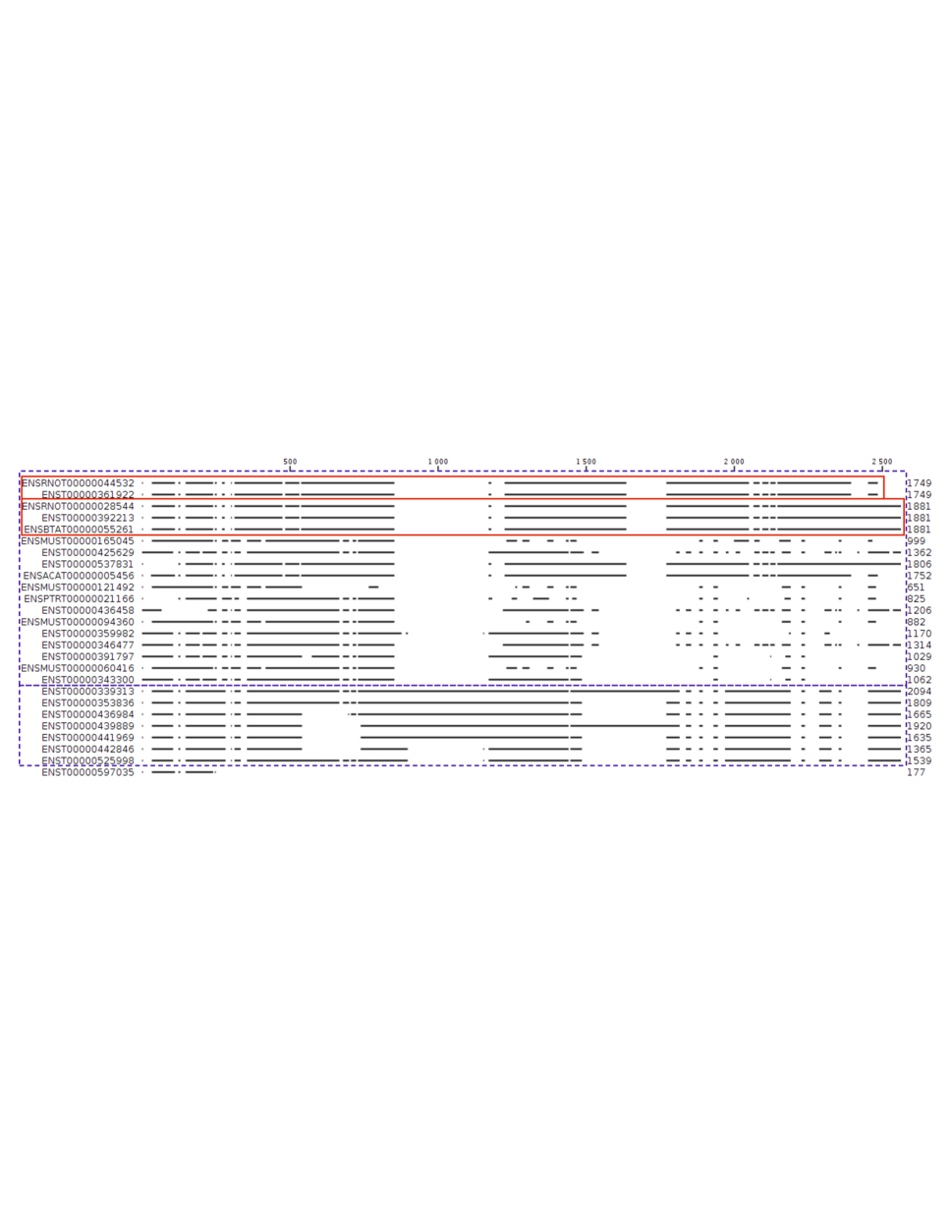
Figure 5: The sets of ortholog clusters obtained using the SFA and the OrthoMCL methods for the MAG family.

The sets of ortholog clusters computed by the two methods are depicted in Figures 5 and 5 in Appendix. For FAM86, SFA allows to recover a $5$-CDS ortholog group composed of CDS conserved across 2 human, 1 mouse, 1 rat and 1 cow genes. It also returns a pair of orthologous CDS from 2 orthologous human and chimpanzee genes. For the MAG family, SFA allows to recover a $3$-CDS ortholog group with CDS from 1 human, 1 rat and 1 cow genes, and a pair of orthologous CDS from 2 orthologous human and rat genes. The multiple alignment of the corresponding protein sequences confirms the accuracy of the ortholog groups (data not shown). The structural similarity between the orthologous CDS is also highlighted in Figures 5 and 5 (Appendix). Concerning the comparison between the OrthoMCL and SFA clusters, for FAM86, SFA returns $9$ clusters and OrthoMCL returns $5$ clusters. For MAG, SFA returns $23$ clusters while OrthoMCL returns $3$ clusters. In both cases, the two sets of clusters are compatible as the clusters computed by the SFA methods are included in larger clusters computed by OrthoMCL. Figures 5 and 5 (Appendix) reveals that the SFA clusters merged by OrthoMCL share some sequence similarities indeed, but they also have different exon structures.

3. Evaluation of the multiple spliced alignment: We applied our multiple spliced alignment algorithm using the pairwise spliced alignments as input. Next, we computed a set of ortholog and close paralog groups, and a multiple alignment of the CDS sequences using the methods described in Section 5. First, we wanted to evaluate the accuracy of the clusters reconstructed based on the multiple spliced alignment and their compatibility with the clusters reconstructed using the more stringent method based on pairwise spliced alignments. For both families, all pairwise SFA clusters are included in larger clusters defined using the multiple SFA clustering method (data not shown). Second, we wanted to evaluate the accuracy of the reconstructed multiple CDS alignments. To do so, we compare them with the multiple CDS alignments obtained using the only existing tools MACSE [14] that allows to align multiple CDS sequences while accounting for translational frameshifts. MACSE [14] was ran with its default parameter values to compute a multiple CDS alignment for each of the gene families. For each gene family, we compare the two CDS multiple alignments, the one from our method SFA and the one from MACSE, based on two criteria which are the percentage of column identity in the alignment and the ratio of long gaps in the alignment that correspond to real exon-exon junctions in the CDS sequences. We define a long gap as a gap of length greater or equal to $20$ between two nucleotides $x[i]$ and $x[i+1]$ of a CDS sequence $x$ in the multiple CDS alignment. This gap corresponds to a real exon-exon junction in the CDS if $x[i]$ and $x[i+1]$ belong to two different (consecutive) exons in $x$.

The results are shown in Table 3 in Appendix. In all cases, SFA recovers a higher number and a higher ratio of long gaps corresponding to real exon junctions in the CDS sequences.

7 Conclusion

This paper introduces a new constrained version and an extended version of the Spliced Alignment Problem for the purpose of identifying CDS ortholog groups within a set of CDS from homologous genes, and for computing multiple CDS alignments. We have developed a variety of algorithmic solutions for the computation of pairwise and multiple spliced alignments. We show how this framework can be used to improve the definition of CDS orthology clusters and multiple CDS alignments. The application of the algorithms to real datasets shows that the framework is particularly useful for identifying CDS ortholog groups that are conserved accross phylogenetically distant genes.

On the algorithmic side, the new problems presented require a more in-depth investigation. For instance, the heuristic algorithm described for the constrained spliced alignment problem could make use of a exact global alignment method with scoring schemes defined to account for all the constaints of the alignments. The heuristic algorithm described for the multiple spliced alignment problem follows a classical greedy approach used by most multiple sequence aligner based on pairwise alignment. What is the complexity of the problem ? It can be seen as a problem of reconstructing a macroscopic multiple alignment and then it is likely to be NP-hard. If so, it is possible that the problem is fixed-parameter tractable with respect to a parameter such as the maximum number of blocks in a pairwise alignment or the maximum size of a conflicting set of blocks. Future work will also make use of benchmark datasets in order to confirm the experimental results of this study.

Appendix

Table 1: Detailed description of the two sets of genes and CDS used for the application.

	Family
	FAM86		MAG
Species	Gene_ID	#CDS	Gene_ID	#CDS
Human	ENSG00000158483 ENSG00000186523 ENSG00000145002	3 4 2	ENSG00000105492 ENSG00000142512 ENSG00000105695	6 7 4
Chimpanzee	ENSPTRG00000007738	1	ENSPTRG00000011374	1
Mouse	ENSMUSG00000022544	1	ENSMUSG00000051504	4
Rat	ENSRNOG00000002876	1	ENSRNOG00000021023	2
Cow	ENSBTAG00000008222	1	ENSBTAG00000017044	1
Chiken	ENSGALG00000002044	1
Lizard			ENSACAG00000005408	1
Total	8 genes	14	8 genes	26

For each gene family, the family identifier, the Ensembl identifier of the genes, the number of complete CDS for each gene and the species of genes are given.

Table 2: Results for the comparison of SFA with the pairwise spliced alignment method SPlign [9].

	Method	Family
		FAM86	MAG
(A)	SFA_0.0 SFA_0.6 SFA_0.7 SFA_0.75 SPlign_0.0 SPlign_0.75	0.91 0.80 0.71 0.65 0.75 0.40	0.42 0.33 0.24 0.22 0.32 0.20
(B)	SFA_0.0 SFA_0.6 SFA_0.7 SFA_0.75 SPlign_0.0 SPlign_0.75	0.56 0.55 0.56 0.56 0.51 0.59	0.45 0.47 0.53 0.53 0.38 0.54
(C)	SFA_0.0 SFA_0.6 SFA_0.7 SFA_0.75 SPlign_0.0 SPlign_0.75	0.79 0.77 0.76 0.75 0.71 0.74	0.77 0.80 0.88 0.90 0.62 0.89
(D)	SFA_0.0 SFA_0.6 SFA_0.7 SFA_0.75 SPlign_0.0 SPlign_0.75	0.94 0.93 0.93 0.92 0.88 0.96	0.90 0.91 0.95 0.96 0.75 0.98

For each method and value of the min_idty parameter, the number correspond to (A) the overall CDS coverage of the spliced alignments and the ratio of internal block extremities (all block extremities except the start of the first block and the end of the last block in a spliced alignment) that correspond to (B) an actual CDS exon extremity, (C) an actual gene exon extremity and (D) a canonical splice site are given.

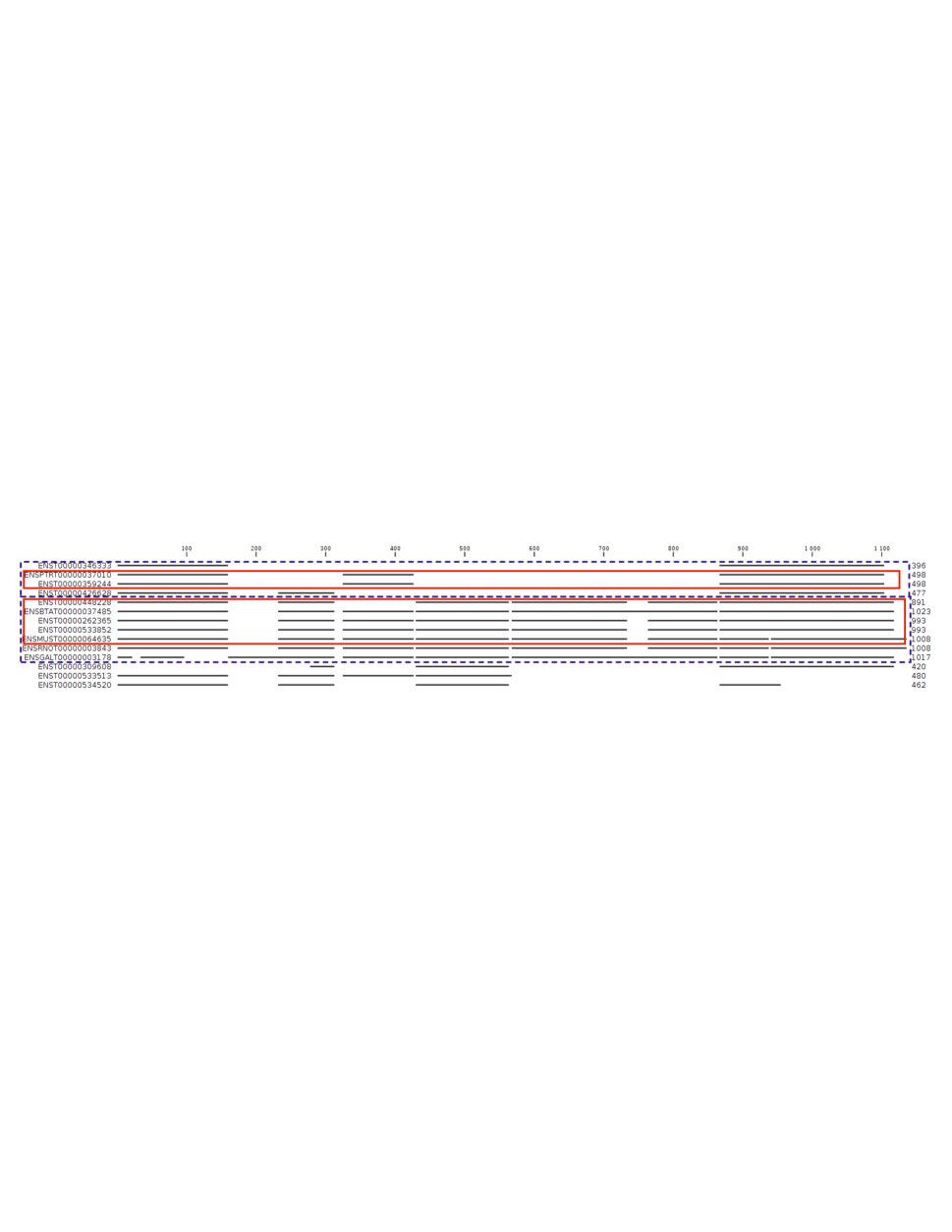
Figure 4: The sets of ortholog clusters obtained using the SFA and the OrthoMCL methods for the FAM86 family. The clusters containing more than one CDS are depicted in red color for the SFA method, and in dotted blue colored line for OrthoMCL. The visualization of the alignment was generated using CLC Sequence Viewer [11]

.

Table 3: Results for the comparison of SFA with the method MACSE [14] for multiple CDS alignment.

Gene family	Methods	(A)	(B)
FAM86	SFA_0.0	0.49	0.81
	SFA_0.5	0.49	0.81
	SFA_0.6	0.56	0.86
	SFA_0.7	0.82	0.82
	SFA_0.75	0.84	0.82
	MACSE	0.47	0.29
MAG	SFA_0.0	0.63	0.57
	SFA_0.5	0.73	0.48
	SFA_0.6	0.74	0.65
	SFA_0.7	0.92	0.84
	SFA_0.75	0.93	0.80
	MACSE	0.44	0.05

For each method, the number correspond to (A) the percentage of columns identity in the multiple CDS alignments and (B) the overall number of long gaps corresponding to real introns divided (/) by the total number of long gaps.

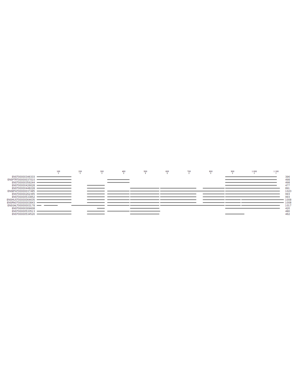
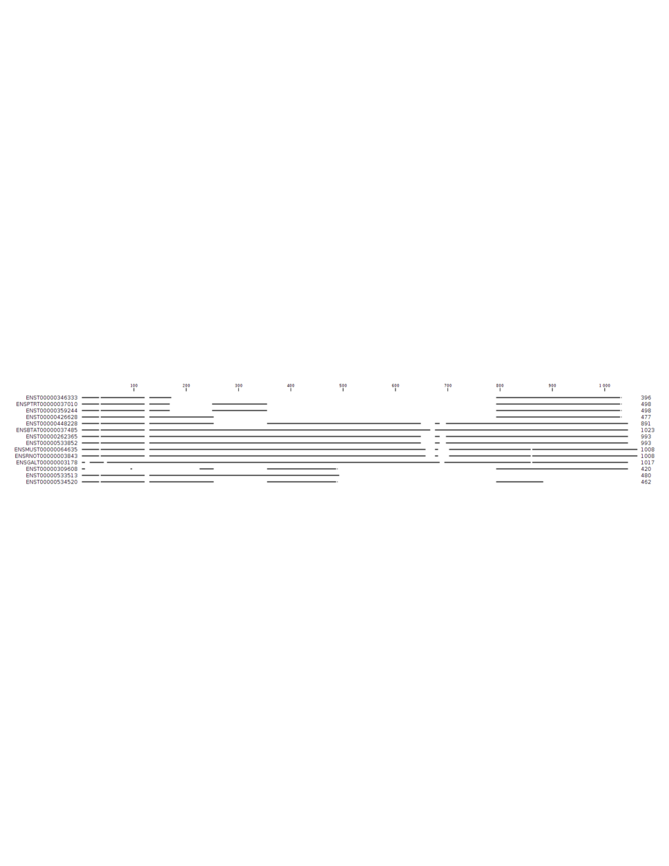
Figure 6: The multiple CDS alignment obtained using the SFA method for the FAM86 family. The visualization of the alignment was generated using CLC Sequence Viewer [11].

Figure 7: The multiple CDS alignment obtained using the MACSE method [14] for the FAM86 family.

References

- [1] Samuel Blanquart, Jean-Stéphane Varré, Paul Guertin, Amandine Perrin, Anne Bergeron, and Krister M Swenson. Assisted transcriptome reconstruction and splicing orthology. BMC Genomics, 17(10):157, 2016.
- [2] Volker Brendel, Liqun Xing, and Wei Zhu. Gene structure prediction from consensus spliced alignment of multiple ests matching the same genomic locus. Bioinformatics, 20(7):1157–1169, 2004.
- [3] M Burset, IA Seledtsov, and VV Solovyev. Analysis of canonical and non-canonical splice sites in mammalian genomes. Nucleic Acids Research, 28(21):4364–4375, 2000.
- [4] Yann Christinat and Bernard ME Moret. A transcript perspective on evolution. IEEE/ACM Transactions on Computational Biology and Bioinformatics, 10(6):1403–1411, 2013.
- [5] Fiona Cunningham, M Ridwan Amode, Daniel Barrell, et al. Ensembl 2015. Nucleic Acids Research, 43(D1):D662–D669, 2015.
- [6] Robert C Edgar. Muscle: multiple sequence alignment with high accuracy and high throughput. Nucleic Acids Research, 32(5):1792–1797, 2004.
- [7] Pär G Engström, Tamara Steijger, Botond Sipos, Gregory R Grant, André Kahles, Gunnar Rätsch, Nick Goldman, Tim J Hubbard, Jennifer Harrow, Roderic Guigó, et al. Systematic evaluation of spliced alignment programs for rna-seq data. Nature methods, 10(12):1185–1191, 2013.
- [8] Mikhail S Gelfand, Andrey A Mironov, and Pavel A Pevzner. Gene recognition via spliced sequence alignment. Proceedings of the National Academy of Sciences, 93(17):9061–9066, 1996.
- [9] Yuri Kapustin, Alexander Souvorov, Tatiana Tatusova, and David Lipman. Splign: algorithms for computing spliced alignments with identification of paralogs. Biology direct, 3(1):20, 2008.
- [10] Hadas Keren, Galit Lev-Maor, and Gil Ast. Alternative splicing and evolution: diversification, exon definition and function. Nature Reviews Genetics, 11(5):345–355, 2010.
- [11] B Knudsen, T Knudsen, M Flensborg, H Sandmann, M Heltzen, A Andersen, M Dickenson, J Bardram, PJ Steffensen, S Mønsted, et al. Clc sequence viewer. A/S Cb, version, 6(2), 2011.
- [12] Esaie Kuitche, Manuel Lafond, and Aïda Ouangraoua. Reconstructing protein and gene phylogenies by extending the framework of reconciliation. Proceedings of International Conference on Bioinformatics and Computational Biology (BICOB’17), (ISBN:9781510836679):79–86, 2017.
- [13] Li Li, Christian J Stoeckert, and David S Roos. Genome research, 13(9):2178–2189, 2003.
- [14] Vincent Ranwez, Sébastien Harispe, Frédéric Delsuc, and Emmanuel JP Douzery. MACSE: Multiple Alignment of Coding SEquences accounting for frameshifts and stop codons. PLoS One, 6(9):e22594, 2011.
- [15] Michael E Sparks and Volker Brendel. Incorporation of splice site probability models for non-canonical introns improves gene structure prediction in plants. Bioinformatics, 21(Suppl_3):iii20–iii30, 2005.
- [16] Thomas D Wu and Colin K Watanabe. Gmap: a genomic mapping and alignment program for mrna and est sequences. Bioinformatics, 21(9):1859–1875, 2005.
- [17] Federico Zambelli, Giulio Pavesi, Carmela Gissi, David S Horner, and Graziano Pesole. Assessment of orthologous splicing isoforms in human and mouse orthologous genes. BMC Genomics, 11(1):1, 2010.