On Dynamic Precision Scaling

Abstract

Based on the observation that application phases exhibit varying degrees of sensitivity to noise (i.e., accuracy loss) in computation during execution, this paper explores how Dynamic Precision Scaling (DPS) can maximize power efficiency by tailoring the precision of computation adaptively to temporal changes in algorithmic noise tolerance. DPS can decrease the arithmetic precision of noise-tolerant phases to result in power savings at the same operating speed (or faster execution within the same power budget), while keeping the overall loss in accuracy due to precision reduction bounded.

*Serif Yesil is now at University of Illinois, Urbana-Champaign; Ismail Akturk, at University of Missouri, Columbia.

1 Introduction

Practical stagnation in voltage scaling renders an increasing chip power density (power per area) over technology generations. At the same time, cooling and power delivery limitations prevent a proportional expansion of the chip power budget. The only way to sustain performance improvement in this environment is enhancing power efficiency, i.e., performance gain per unit power consumed [Horowitz (2014)]. Approximate computing is a promising paradigm which can enhance power efficiency by trading computation accuracy for performance or power, depending on the tolerance of algorithms to noise (i.e., accuracy loss) in computation. The intrinsic noise tolerance of the emerging R(ecognition), M(ining), and S(ynthesis) applications [Chen et al. (2008)] – which process massive but noisy input data by probabilistic algorithms (often featuring iterative refinement) – makes them particularly suitable to approximate computing.

Approximate computing by precision reduction represents a heavily explored area of research [Yeh et al. (2007), Esmaeilzadeh et al. (2012), Sampson et al. (2011)]. In this paper, we explore approximation by adaptive precision reduction, a relatively less explored area. Specifically, based on the observation that applications exhibit varying degrees of sensitivity to noise during computation, we explore how tailoring the precision of computation adaptively to temporal changes in algorithmic noise tolerance can maximize power efficiency.

Due to its analogy to Dynamic Voltage and Frequency Scaling (DVFS), we refer to this paradigm as Dynamic Precision Scaling (DPS). Recall that DVFS can maximize power efficiency by tracking temporal changes in the performance demand of the workload (which in turn evolves as a function of temporal changes in computation and memory access characteristics) and by changing the operating point (i.e., the operating voltage and frequency) accordingly. Similar to DVFS, DPS tracks temporal changes in workload characteristics. However, in maximizing power efficiency, contrary to DVFS, DPS exploits temporal changes in noise tolerance, and adaptively decreases the arithmetic precision of noise-tolerant phases to obtain power savings at the same operating speed (or faster execution within the same power budget) while keeping the overall loss in accuracy due to precision reduction bounded. Conceptually, for less noise-tolerant phases, DPS can adjust the arithmetic precision on the fly to prevent excessive loss in computation accuracy.

In this paper, we conduct a limit study in order to quantify the power efficiency potential of DPS. To this end, we devise a proof-of-concept implementation of the DPS concept. Specifically, we first develop a workload analyzer which can identify application phases of varying noise tolerance. Then, using the outcome of this workload analyzer, we design two heuristic DPS policies. In the following, Section 2 introduces DPS basics and the two proof-of-concept policies; Sections 3 and 4 provide the evaluation; Section 5 covers related work; and Section 6 summarizes our findings.

2 Dynamic Precision Scaling (DPS)

2.1 Dynamic Precision Scaling: Basics

To be able to tune the arithmetic precision of computation on the fly, any practical DPS implementation has to monitor fine grain temporal changes in the noise tolerance of the workload. Noise tolerance of emerging RMS applications stems from (i) algorithms which are mostly probabilistic and often utilize iterative refinement; (ii) inputs which contain a very large number of noisy (and often redundant) elements. Due to (i), it is barely possible to differentiate noise tolerant phases from others without understanding program semantics. On the other hand, (ii) renders profiling-based identification of noise tolerant phases inevitable, as explored in [Khudia et al. (2015), Ringenburg et al. (2015)].

Based on these observations, we envision a practical DPS implementation to comprise three basic modules: an offline profiler, a runtime monitor, and an accuracy controller. The differences in the design of these three modules give rise to different points in the DPS design space. The offline profiler not only identifies but also demarcates noise tolerant application phases, such that the runtime monitor can detect on the fly which phases of the application are more noise tolerant and which are less. Finally, the accuracy controller processes the output of the runtime monitor to adjust the arithmetic precision on the fly. Similar to DVFS controllers, the accuracy controller is in charge of scheduling decisions for timely precision scaling.

The underlying hardware architecture can harvest power efficiency from DPS in numerous ways. For example, arithmetic units of reconfigurable precision represent a good match for DPS. Narrow operand widths under lower precision arithmetic can result in higher power efficiency due to the increased processing speed along with power savings [Tong et al. (2000)]. However, in mapping (more) noise-tolerant phases to arithmetic units of reduced precision, particularly under fine-(temporal)-grain DPS, the accuracy controller has to carefully budget for the power and performance overhead of the scheduling decisions.

In the following, we will detail a proof-of-concept DPS implementation which features an offline profiler along with a hypothetical runtime monitor and an accuracy controller. This implementation primarily serves automated design space exploration with limited user input which enables the application programmer and system designer to exploit temporal variations in the noise-tolerant phases of computation.

2.2 A Proof-of-Concept DPS Implementation

Without loss of generality, we confine the proof-of-concept DPS implementation to the floating point datapath. However, the DPS concept generally applies to the integer datapath, as well, where the main complication comes from identification, and hence, exclusion of memory address calculations (i.e., pointer arithmetic) from approximation.

We reduce precision by omitting a subset of less significant bits of the fraction: According to the IEEE 754 standard, a single (double) precision floating point number occupies an 32(64)-bit register with one bit allocated for sign, 8 (11) bits for exponent, and 23 (52) bits for fraction, i.e., mantissa, respectively. A single precision floating point number, e.g., corresponds to $(-1)^{sign}\times 2^{exponent-127}\times 1.mantissa$.

Input: targetAccLoss, #bits, #dynamicCalls

Input: AccLossS0[1…#dynamicCalls][1..#bits]

Input: AccLossS1[1…#dynamicCalls][1..#bits]

Output: #omittedBits[1…#dynamicCalls]

1

2for i$\leftarrow$1…#dynamicCalls  do

3      $targetBit\leftarrow 0$ ;

4      $cummAccLoss\leftarrow 0$ ;

5      while cummAccLoss$<$targetAccLoss & targetBit$\leq$#bits do

6          

7          if AccLossS0[i][targetBit] and AccLossS1[i][targetBit] are valid  then

8                $err\leftarrow\max(AccLossS0[i][targetBit],AccLossS1[i][targetBit])$ ;

9                $cummAccLoss+\leftarrow err$ ;

10               

11                else

12                     $break$;

13                    

14                     end if

15                    $targetBit++$;

16                    

17                     end while

18                    $\#omittedBits[i]\leftarrow targetBit-1$;

19                    

20                     end for

ALGORITHM 1 Basic DPS Policy

Input: targetAccLoss, #bits, #dynamicCalls

Input: AccLossS0[1…#dynamicCalls][1..#bits]

Input: AccLossS1[1…#dynamicCalls][1..#bits]

Output: #omittedBits[1…#dynamicCalls]

1

2for i$\leftarrow$1…(#dynamicCalls-1)  do

3      $targetBit\leftarrow 0$ ;

4      $cummAccLoss\leftarrow 0$ ;

5      cummAccLoss_next $\leftarrow$ 0;

6     

7     while cummAccLoss$<$targetAccLoss & targetBit$\leq$#bits
& cummAccLoss_next$<$targetAccLoss  do

8           if AccLossS0[i][targetBit], AccLossS1[i][targetBit],
AccLossS0[i+1][targetBit], AccLossS1[i+1][targetBit] are valid  then

9                $err\leftarrow\max(AccLossS0[i][targetBit],AccLossS1[i][targetBit])$ ;

10                err_next $\leftarrow\max$ (AccLossS0[i+1][targetBit], AccLossS1[i+1][targetBit]) ;

11                $cummAccLoss+\leftarrow err$ ;

12                $cummAccLoss\_next+\leftarrow err\_next$ ;

13               

14                else

15                     $break$;

16                    

17                     end if

18                    $targetBit++$;

19                    

20                     end while

21                    $\#omittedBits[i]\leftarrow targetBit-1$;

22                    

23                     end for

24                    

ALGORITHM 2 Dependency-Aware DPS Policy: DPS+

The proof-of-concept implementation captures temporal changes in application's noise tolerance by tracking (dynamic) calls to floating point heavy functions within the course of execution. Dynamic function calls, i.e., different invocations of a given (static) function, are dispersed in time within the course of execution, and therefore can reflect temporal changes in noise tolerance. Without loss of generality, DPS can track temporal changes in application's noise tolerance at various granularities (such as instruction or basic block), giving rise to different implementations. The proof-of-concept design works at function granularity, and uses dynamic function calls to capture the notion of time. In other words, the proof-of-concept design employs noise tolerant dynamic calls as proxies for noise tolerant phases of the application. In this case, the question becomes how to identify noise-tolerant dynamic function calls.

To this end, the offline profiler module in the proof-of-concept implementation uses a two-step approach: The first step involves statistical fault injection; the second step, post-processing of statistical fault injection results. At the first stage, for each dynamic invocation of each floating point heavy function, we corrupt one mantissa bit at a time and record the corresponding accuracy loss at the application output. We repeat this experiment for all mantissa bits, by injecting both stuck-at-0 and stuck-at-1 faults. We corrupt all floating point variables in the function, in the same direction. Recall that the proof-of-concept implementation uses noise tolerant dynamic calls as proxies for noise tolerant phases of the application. The accuracy loss observed in the end result per fault injection experiment serves as a proxy for the degree of noise tolerance of each dynamic call. The offline profiler also needs to communicate this information to the runtime.

The post-processing step can rely on different policies. We first devise a basic DPS policy following Algorithm 1: The key inputs of this algorithm are targetAccLoss, the maximum accuracy loss in the end result the application can tolerate; and the outcome of the first step of offline profiling, namely the accuracy loss observed in the end result after injecting stuck-at-0 and stuck-at-1 faults in each mantissa bit of each dynamic invocation of a floating point heavy function. #bits specifies the number of mantissa bits subject to fault injection, and #dynamicCalls, the number of dynamic (floating point heavy) function calls (which may cover different static functions). We keep the fault injection information in two separate (#dynamicCalls$\times$#bits) matrices for stuck-at-0 (AccLossS0) and stuck-at-1 faults (AccLossS1). The output is the total number of (consecutive) mantissa bits (starting from the least significant) we can omit while the corresponding accuracy loss in end result remains lower than targetAccLoss, on a per dynamic call basis: #omittedBits.

Each step of the algorithm processes a different dynamic call (line 1). Starting from the least significant bit, we check the accuracy loss in the end result under the corruption of each mantissa bit (i.e., targetBit): If the corresponding AccLossS0(1) entries are valid, i.e., the fault injection experiment did not result in Inf or NaN (line 5), we extract the maximum of accuracy loss under stuck-at-0 and stuck-at-1 (line 6). This basic DPS policy accumulates this maximum accuracy loss in the end result due to the corruption of each mantissa bit in isolation (in cummAccLoss from line 7), as we consider more mantissa bits for omission. cummAccLoss serves as a running estimate for the actual accuracy loss in the end result. Accordingly, the policy keeps processing higher-order mantissa bits for omission as long as cummAccLoss remains below targetAccLoss (line 4).

A runtime monitor can then use the output of the basic DPS policy captured by Algorithm 1, #omittedBits, to tune the precision of each dynamic function call on the fly. Algorithm 1's main bottleneck, however, is cummAccLoss, the estimate of cumulative accuracy loss in the end result of the application if we omit multiple mantissa bits (line 7). This is because the actual (runtime) impact of each omitted mantissa bit on the accuracy loss in the end result may not always be additive. Therefore, in the worst case, if we omit multiple mantissa bits following Algorithm 1 – as captured by #omittedBits – we may eventually observe a higher accuracy loss in the end result than targetAccLoss. A refined version of the basic DPS policy, DPS+, can mitigate this, as depicted in Algorithm 2  (with the difference between the two algorithms highlighted).

Both algorithms process all dynamic function calls within the course of execution; the order of the dynamic calls in AccLossS0(1) and #omittedBits arrays reflect their execution order in the offline profiling run. These dynamic calls may cover more than one static (floating point heavy) function. For the representative set of RMS benchmarks we experiment with (Section 3), we observe that dynamic calls following each other in dynamic control flow are often also data dependent. Algorithm 2 leverages this insight by limiting the precision reduction of a dynamic function to the precision reduction of its follower function in execution (and processing) order. In this manner, we enforce that the (reduced) precision of a producer's output data matches (i.e., does not exceed) the maximum acceptable precision of the input data of its (immediate) consumer.

Algorithm 2 still cannot provide mathematical guarantees (as data dependent functions are not always executed back to back), but can effectively enforce runtime accuracy loss (in the end result) to remain below targetAccLoss. Algorithm 2 can further be refined by tracking actual call graphs, similar to [Stephenson et al. (2000)], of data dependent dynamic functions for precision matching.

3 Evaluation Setup

Table 1: List of benchmarks used.

Benchmark	Description	Input Dataset
Blackscholes (BS) [Bienia et al. (2008)]	PDE solver	simsmall
Fluidanimate (FA) [Bienia et al. (2008)]	n-body simulation	simsmall
Hotspot (HS) [Che et al. (2009)]	Thermal simulation	64x64 grid
Particlefilter (PF) [Che et al. (2009)]	Medical imaging	128x128 10 timepoints
Pagerank (PR) [Beamer et al. (2015)]	Graph processing	gnutella04
		[Leskovec and Krevl (2014)]

Throughout the evaluation, we will refer to the proof-of-concept implementation as DPS(+).

3.1 Benchmarks

To quantify the power efficiency potential of DPS, we deploy a representative, relatively floating point heavy, set of RMS applications from PARSEC [Bienia et al. (2008)], Rodinia [Che et al. (2009)] and Gapbs [Beamer et al. (2015)] suites, as captured by Table 1. We deploy default input data sets except Pagerank (PR). The inputs for PR come from a well-known graph database [Leskovec and Krevl (2014)].

Blackscholes (BS) calculates stock option prices solving Partial Differential Equations (PDE). While the application domain is arguably not suitable for approximation, we included the benchmark as a representative PDE solver. The region of interest, ROI (where the actual computation takes place), comprises the function BlkSchlsEqEuroNoDiv. Each function call calculates the price of a different stock option, hence errors in a call can only affect the corresponding stock price, but not other calls. Fluidanimate (FA) represents n-body simulation, where bodies correspond to fluid particles. The ROI comprises four relatively floating point heavy functions: RebuildGrid, ComputeForces, ProcessCollisions, AdvanceParticles. Hotspot (HS) is an architectural thermal simulator. The ROI comprises a kernel to compute the temporal temperature difference (i.e., delta) at each sampled location in a processor chip, encapsulated in find_delta function. Particlefilter (PS) is a medical imaging application to track an object in an image. The ROI comprises particleFilter function. The main work of this function is carried out in a loop that iterates over frames. Every iteration calls five relatively floating point heavy functions subject to DPS: apply_motion_model, particle_filter_likelihood, update_weights, normalize_weights, and calc_U. Pagerank (PR) is an iterative graph algorithm. At every iteration, pagerank_calculate function traverses all vertices of a given web graph and calculates the PageRank of an individual vertex by summing weighted PageRank values of its neighbors.

All benchmarks output (possibly multi-dimensional) numeric values. To quantify the accuracy loss in the end result under DPS, we use mean relative error (i.e., average relative error over all data points in the output) with respect to the full-precision outcome. The data points in BS are final stock option prices; in FA, final positions of cells; in HS, temperature values; in PF, the final position of the object being tracked; in PR, the PageRank values of each vertex.

As explained in Section 2.2, in our experiments time advances with each dynamic function call – in other words, we use dynamic function calls – every call to the aforementioned floating point heavy functions – as (not necessarily always homogeneous) units in time.

We experiment with single-threaded binaries. For FA, PS and PR, the functions subject to DPS distribute work to threads, hence DPS can expand to parallel execution in a seamless fashion, by imposing the same precision reduction over all threads. For BS and HS, on the other hand, the functions subject to DPS can run in parallel, so different threads may invoke the same function with different precision simultaneously. We leave further exploration to future work.

3.2 Simulation Infrastructure

We implement the proof-of-concept offline profiler compromising statistical fault injection and DPS policies using Pin [Luk et al. (2005)], as an extension to the Pin-based approximate computing framework iACT [Mishra et al. (2014)]. During offline profiling, we inject two types of faults in the mantissa: We set one mantissa bit (out of 23 for single; 52, for double precision) to 0 (stuck-at-0) or 1 (stuck-at-1) at a time. Our tool instruments all floating point arithmetic and load/store instructions for DPS(+). We compiled the benchmarks using gcc4.9, and disabled SIMD extensions. In accordance with the energy model presented in [Shao and Brooks (2013)], we experimented with a Xeon-Phi like core of 32KB L1 data cache and 512KB L2 data cache.

3.3 Energy Model

To model energy, we use sum of products of energy per instruction ($EPI$) and number of instructions ($\#instructions$), over each instruction category (in each dynamic function call). EPI estimates come from measured data from [Shao and Brooks (2013)], which categorize instructions according to the sources of operands as RF (register file), L1, L2 (level-1 or -2 cache) and (main) memory. [Shao and Brooks (2013)] not only provides robust, measurement based EPI estimates, but also is suitable for our exploration based on the x86 instruction set architecture (due to the utilization of Pin). In this work, we do not consider vector optimizations, and use scalar operation EPI values from [Shao and Brooks (2013)], as summarized in Table 2.

Table 2: EPI values used in this study.

Instruction Category ($C$) based on operand source	$EPI_{C}$ (nJs)
RF (register file)	0.45
L1	0.88
L2	7.72
Memory Read (Rd) (with prefetch)	52.14
Memory Write (Wr)	62.14

To calculate the energy consumption of each dynamic function call, we first determine the number of instructions in each (operand source based) category, following the classification in Table 2. Under full precision, the energy consumed by each category in a dynamic function call becomes

$$EPI_{C}\times\#instructions_{C}$$

where $C$ represents the category, i.e., RF, L1, L2 or Memory (Rd or Wr); $EPI_{C}$, the EPI estimate of the instructions in category $C$, and $\#instructions_{C}$, the number of instructions in the dynamic function call which fall into category $C$.

Notice that not all of the floating point instructions are subject to precision reduction under DPS(+). $EPI_{C}$ values of instructions which keep full precision directly come from Table 2 [Shao and Brooks (2013)]. For the instructions subject to omission of mantissa bits of their operands under DPS(+), on the other hand, EPI changes as a function of the number of (mantissa) bits omitted – we will refer to this function as $EPI_{C,o}$. Hence, the energy consumed by each category $C$ in a dynamic function call becomes

$$EPI_{C}\times\#instructions_{C,no}+EPI_{C,o}\times\#instructions_{C,o}$$

$$~{}~{}~{}\texttt{with}~{}~{}~{}\#instructions_{C}=\#instructions_{C,no}+\#instructions_{C,o}$$

where $\#instructions_{C,no}$ ($\#instructions_{C,o}$) represents the number of instructions in the dynamic function call which fall into category $C$ and where no (a subset of the) operand mantissa bits are omitted. $EPI_{C,o}$ changes with the number of omitted bits.

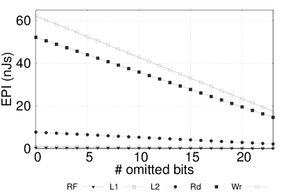
(a) Single Precision

(b) Double Precision

Figure 1: EPI as a function of the number of mantissa bits omitted.

We deploy the scaling model from [Tong et al. (2000)] to model how $EPI_{C,o}$ changes as a function of the number of mantissa bits omitted. In [Tong et al. (2000)], the authors show that in floating point multiplication, which represents one of the most energy hungry floating point operations, processing mantissa bits can easily consume more than $\approx$80% of the total energy. This study provides a first order analysis of the energy impact of reducing mantissa precision, considering energy per operation. The authors implement a digit-serial multiplier and extract its energy consumption from SPICE simulation. The key finding is that energy per operation increases linearly with the operand bit-width. This multiplier can also serve as a mantissa multiplier. In this case, the energy consumption increases mostly linearly with the number of mantissa bits. In the following, we stick to this linear model. Fig. 1 shows how $EPI_{C,o}$ changes with number of omitted mantissa bits, for each category $C$, considering single (a) and double (b) precision.

The linear scaling model from Fig. 1 provides enough confidence for a limit study to quantify the power efficiency potential for DPS(+), the goal of this paper. Accordingly, we do not tie our evaluation to any specific hardware implementation. While the picture in Fig. 1 is likely to hold asymptotically, it will change depending on whether the underlying hardware features functional units of reduced precision or functional units of reconfigurable precision.

In the following, we will report the cumulative energy savings in the ROI of the benchmark applications (where the actual computation takes place) under DPS(+), and not just in the floating point datapath.

(a) BS

(b) FA

(c) HS

(d) PR

(e) PF

Figure 2: Statistical fault injection outcome for temporal noise tolerance. Bit 23 on the x-axis demarcates the most significant; bit 0, the least significant.

4 Evaluation

4.1 Application Characteristics

Table 3 captures the share of F(loating) P(oint) operations in the instruction mix and energy consumption of the RMS benchmarks deployed, over the entire region of interest (ROI). We observe that the energy share of FP operations in ROI ranges from 12% (PF) to 29% (BS). These numbers provide an upper bound for energy savings under DPS(+).

Table 3: Ratio of FP operations in instruction mix & energy consumption.

Benchmark	FP ops. in ROI	FP energy in ROI
BS	0.25	0.29
FA	0.15	0.13
HS	0.12	0.17
PF	0.10	0.12
PR	0.05	0.13

Fine grain temporal changes in the noise tolerance of RMS applications motivates DPS(+). Fig. 2 verifies this insight, where we plot the outcome of the fault injection experiments to measure the sensitivity of each FP-heavy dynamic function call to noise. The x-axis depicts which mantissa bit we corrupt. The left y-axis shows the dynamic function calls, in the order of execution (as identified during profiling). The right y-axis captures the (relative) accuracy loss in the end result as induced by the corrupted bit in gray scale (black indicates a totally inaccurate result, i.e., a relative accuracy loss of 1; white, no accuracy loss). As expected, we observe more darker regions (less noise tolerance) as we move right on the x-axis – as we corrupt higher order (more significant) mantissa bits.

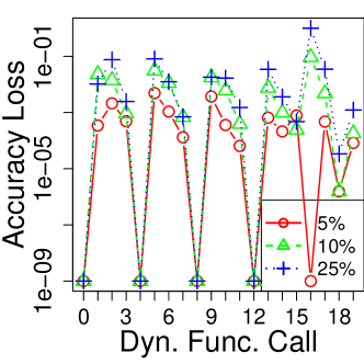
(a) FA

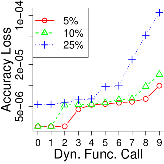
(b) PR

Figure 3: Evolution of noise tolerance with time.

We observe that the accuracy loss (right y-axis) indeed changes with time (i.e., with dynamic function calls as depicted on the left y-axis) for all applications, least pronounced for HS in Fig. 2(c). For the rest of the applications, the accuracy loss (as a proxy of noise tolerance) shows recurring patterns over time: For example, FA (b) periodically enters a relatively more noise tolerant phase (as characterized by AdvanceParticle function); PF (e), a relatively less noise tolerant phase (as characterized by apply_motion_model function). PR (d), on the other hand, exhibits less noise tolerance as we move up on the left y-axis – in later stages of execution. This is because, relying on iterative refinement, PR has less opportunities to recover from noise in later stages of execution. Careful inspection reveals barely any accuracy loss, even due to the corruption of more significant mantissa bits, until sixth iteration. After sixth iteration, however, we start to observe sizable loss in accuracy.

Most of the time, differences in the noise tolerance of each dynamic call to the very same static function stem from differences in the function inputs across calls. For instance, BS has a single computational kernel. Each (dynamic) call to this kernel processes different inputs. Fig. 2(a) reveals the differences in accuracy loss among these calls due to inputs along the time (left y-) axis. Input data values also have an impact. When working with smaller values, corruptions in least significant bits are more likely to induce higher accuracy loss in the end result. This applies to the fluctuations in accuracy loss across the left y-axis due to the corruption after least significant 8 bits in (a). All of these results point to opportunities for DPS.

(a) Accuracy Loss

(b) Energy

Figure 4: Impact of SPS on accuracy loss (a) and energy (b).

Fig. 3 provides the microscopic view for two of the applications from Fig. 2: FA (a) and PR (b). The x-axis corresponds to time (the left y-axis of Fig. 2); the y-axis, to relative accuracy loss (the right y-axis of Fig. 2). In this case, we omit multiple consecutive mantissa bits; specifically, (ceiling of) 5%, 10%, and 25% of mantissa bits, starting from the least significant. In line with our findings from Fig. 2, we identify how the noise tolerance of FA (a) fluctuates; and of PF (b), decreases over time.

4.2 Static Precision Scaling (SPS)

We next explore how the accuracy loss and energy consumption look like if we impose a fixed degree of precision reduction, statically, throughout the entire execution. In the following, we will refer to this policy as Static Precision Scaling (SPS). We will use the outcome under SPS as a baseline for comparison. As SPS does not differentiate between noise tolerance of dynamic calls, the least noise tolerant function is likely to determine the final accuracy loss. Under SPS, we omitted (ceiling of) 5%-75% of mantissa bits. Fig. 4 captures the outcome. We observe that SPS can render sizable energy savings (b), particularly as we omit more than 10% of the bits. However, for BS and FA the energy savings are accompanied by the excessive accuracy loss as revealed in (a). According to Fig. 2, FA can tolerate corruption in higher order bits of mantissa, but SPS cannot unlock this opportunity. Under SPS, FA renders unacceptable accuracy loss if we omit 25% of the bits (6 bits). In the next section, we will show that FA can tolerate omission of up to 15 bits under DPS (+) (Fig. 5). Similarly, under SPS, BS cannot tolerate the omission of 50% of its mantissa bits (12 bits), where according to Fig. 2, many of its dynamic calls may tolerate corruption at higher order bits (bit 18, e.g.). For the rest of the applications, SPS performs arguably well. Still, DPS(+) can unlock more opportunities for power efficiency: As a specific example, PR under SPS with 75% of mantissa bits (18 bits) omitted results in 0.37$\times$ accuracy loss. According to Fig. 2, PR can temporally tolerate the omission of higher order bits. In the next Section we will show how DPS(+) can unlock this opportunity by omitting 90% of the mantissa bits on average to render an accuracy loss of 0.13$\times$.

4.3 Dynamic Precision Scaling (DPS)

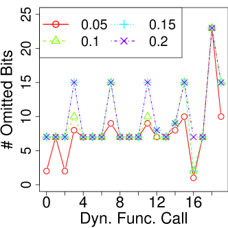
(a) DPS

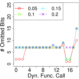
(b) DPS+

Figure 5: #omitted bits under DPS(+) for FA.

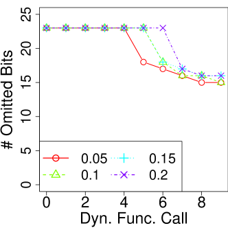
(a) DPS

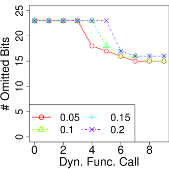
(b) DPS+

Figure 6: #omitted mantissa bits under DPS(+) for PR.

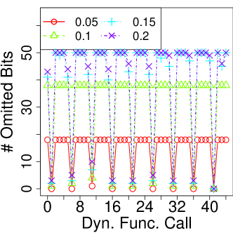
(a) DPS

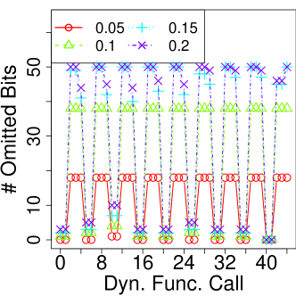
(b) DPS+

Figure 7: #omitted bits under DPS(+) for PF.

We next evaluate the effectiveness of DPS(+). We invoke the two DPS algorithms with different values of targetAccLoss (Section 2.2), the maximum accuracy loss in the end result the application can tolerate, and feed the resulting #omittedBits to the runtime monitor. Recall that #omittedBits gives the total number of (consecutive) mantissa bits (starting from the least significant) we can omit on a per dynamic call basis, while the corresponding accuracy loss in end result remains lower than targetAccLoss. In the following, we report the outcome for targetAccLoss values between 0.05 and 0.2 at increments of 0.05. Fig.s 5, 6, and 7 depict the number of omitted bits for each dynamic function call, as a function of targetAccLoss, for FA, PR, and PF, respectively; under DPS in (a), and DPS+ in (b).

The pattern under DPS closely tracks our findings in Fig. 2, as DPS considers each dynamic call in isolation. This observation also holds for BS and HS, not shown as the corresponding figures were barely readable due to very fine grain temporal fluctuations. Recall that the x-axis captures each dynamic function call in the order of execution, and hence represents a proxy for time. Fig.s 5, 6, and 7, respectively, for FA, PR, and PF, show how the number of omitted bits changes over time to track the temporal changes in the noise tolerance of the applications (more noise-tolerant phases being able to accommodate a higher number of omitted mantissa bits).

We next examine the corresponding accuracy loss in the end result of the applications in Table 4 for DPS, in Table 5 for DPS+, and in Table 6 for DPS_min. We observe that (i) as expected, a higher targetAccLoss value renders monotonically higher accuracy loss for all applications; (ii) the accuracy loss under DPS eventually overshoots targetAccLoss (highlighted in bold); (iii) by dependency tracking, DPS+ manages to eliminate most of the overshoots and to bound the final accuracy loss opportunistically.

At this point, we introduce one more baseline for comparison, SPS+, which can eliminate such overshoots. SPS+ works as follows: During profiling, (i) we first run DPS heuristic to find the number of bits to be omitted for each dynamic function call; (ii) we then find the minimum #omittedBits for each static function by using the profile from (i) over all of its dynamic function calls. After profiling, we impose this number of bits on all dynamic calls throughout execution. As Table 6 reveals, SPS+ renders a lower accuracy loss. However, as SPS+ cannot exploit temporal changes in algorithmic noise tolerance, it leaves potential savings in energy untapped. For example, BS features a single target function, some dynamic instances of which cannot tolerate approximation (i.e., where #omittedBits becomes zero). SPS+ in this case imposes this #omittedBits as the minimum over all dynamic calls, and hence, excludes any approximation. As a result, SPS+ cannot deliver any energy savings for BS as opposed to DPS(+), as we will see shortly in Figure 9.

Table 4: Accuracy loss under DPS for different targetAccLoss values

	0.05	0.1	0.15	0.2
PF	0.0025	0.0028	0.0347	0.7759
HS	0.0036	0.01233	0.2140	0.2140
PR	0.0849	0.1416	0.1714	0.2582
FA	5.63E-5	8.25E-5	8.32E-5	0.0823
BS	0.02907	0.0486	0.0688	0.0769

Table 5: Accuracy loss under DPS+ for different targetAccLoss values

	0.05	0.1	0.15	0.2
PF	0.0025	0.0025	0.0111	0.0111
HS	0.0035	0.0123	0.2120	0.2140
PR	0.0758	0.0848	0.1428	0.1646
FA	9.66E-6	2.64E-5	2.64E-5	0.0822
BS	0.0234	0.0419	0.0605	0.0682

Table 6: Accuracy loss under SPS+ for different targetAccLoss values

	0.05	0.1	0.15	0.2
PF	0.0025	0.0027	0.0110	0.0130
HS	0.0032	0.0066	0.0123	0.2140
PR	0.0615	0.0615	0.1308	0.1308
FA	8.84E-6	8.86E-6	3.30E-5	0.0822
BS	0	0	0	0

PF and PR feature data-dependent consecutive dynamic function calls. Since the output of the preceding function call acts as the input to the next function call, omitting more bits in the preceding call (than the following call) tends to result in higher, and possibly excessive accuracy loss. DPS+ handles this case by matching the precision reduction of consecutive calls. Mainly applications featuring this or similar type of data dependency can benefit from DPS+. As a result, under DPS+, the accuracy loss of PF and PR significantly decreases. For example, at targetAccLoss=0.05, Fig. 6(b) shows how DPS+ matches the number of omitted bits in the 3^rd dynamic function call for PR, due to the significant difference in the noise tolerance of 3^rd and 4^th calls (which is not the case under DPS, as Fig. 6(a) reveals). A similar matching, although less visible, applies for PF, in Fig. 7.

In summary, we observe that DPS+ can effectively bound the accuracy loss, although overshoots still apply for HS under DPS+. To handle these cases, DPS+ can be refined to track the actual call graphs of data dependent dynamic functions for precision matching. Such refinement is also likely to untap even more opportunities, considering the cases in Tables 4, 5 with a large gap between the actual accuracy loss and targetAccLoss.

Figure 8: Energy consumption under DPS for different targetAccLoss values.

Figure 9: Energy consumption under SPS+ for different targetAccLoss values.

Fig. 8 captures energy savings under DPS for targetAccLoss values between 0.05 and 0.2 at increments of 0.05. Savings span 0.09% to 63.8%. Notable energy savings apply to BS, HS, and PR. Savings for FA and PF are modest. DPS(+) excludes floating point instructions from shared libraries, which likely hurts both of these applications. At the same time, for PF, the ratio of $\#instructions_{C,no}/\#instructions_{C,o}$ is around 10, which severely limits energy savings independent of targetAccLoss value. Also, the most energy-hungry dynamic functions feature the lowest number of omitted mantissa bits in Fig. 7.

DPS+ renders less (or at most equal) number of omitted bits when compared to DPS, hence may leave potential energy savings untapped in trying to limit the accuracy loss. However, we find that the maximum difference between energy savings of DPS and DPS+ barely reaches 4.7%. On average, the difference remains around 1.44%.

Figure 9 captures the energy profile under SPS+. Overall, SPS+ renders a higher energy consumption than DPS(+). BS is not the only application which loses the energy benefits of dynamic precision scaling under SPS+. For example, energy consumption of PR increases by 45% when compared to DPS. Overall, the increase in energy consumption varies between 1% to 78% when we consider all applications.

(a) DPS

(b) DPS+

Figure 10: Accuracy loss distribution for BS.

A note on accuracy metric: In quantifying the accuracy loss, we used mean relative error (i.e., mean relative accuracy loss) as a generic accuracy metric, as explained in Section 3. Mean relative error may be misleading if the standard deviation assumes a large value. To quantify the standard deviation, Figures 10–13 depict the distribution of component accuracy loss values (as captured by the legends). The x-axis captures different values of targetAccLoss. For example, for BS, we observe that 84% to 92% of relative accuracy loss values fall below the given targetAccLoss under DPS; and 92% to 98%, under DPS+. A similar trend holds for PR, considering different inputs.

(a) DPS

(b) DPS+

Figure 11: Accuracy loss distribution for PR with gnu04 input set.

(a) DPS

(b) DPS+

Figure 12: Accuracy loss distribution for PR with gnu05 input set.

(a) DPS

(b) DPS+

Figure 13: Accuracy loss distribution for PR with pk input set.

4.4 Input Sensitivity

Table 7: Input Sensitivity Analysis for Pagerank (PR) with different datasets from the Snap Database[Leskovec and Krevl (2014)]. Only gnu04 is deployed for profiling.

		0.05	0.1	0.15	0.2
gnu04	DPS	0.0849	0.1416	0.1714	0.2582
	DPS+	0.0758	0.0848	0.1428	0.1646
	SPS+	0.0615	0.0615	0.1308	0.1308
gnu05	DPS	0.1029	0.1499	0.1805	0.2423
	DPS+	0.0846	0.0988	0.1597	0.1763
	SPS+	0.0764	0.0764	0.1406	0.1406
gnu08	DPS	0.1906	0.2567	0.3232	0.3900
	DPS+	0.1604	0.1857	0.2829	0.3132
	SPS+	0.1400	0.1400	0.2463	0.2463
gnu25	DPS	0.0395	0.0833	0.0986	0.1730
	DPS+	0.0276	0.0391	0.0650	0.0896
	SPS+	0.0244	0.0244	0.0525	0.0525
pk	DPS	0.9107	0.9211	0.9490	0.9524
	DPS+	0.9050	0.9101	0.9452	0.9488
	SPS+	0.8832	0.8832	0.9317	0.9317
wg	DPS	0.9310	0.9572	0.9611	0.9787
	DPS+	0.9019	0.9269	0.9383	0.9508
	SPS+	0.7813	0.7813	0.8839	0.8839

In order to quantify the input dependence due to profiling, we experiment with PR, which features a rich set of inputs. As other profiling based approaches, DPS(+) is input dependent. However, the degree of this dependence changes from application to application. At the same time, when the properties (such as size and value distribution) of two input datasets are close to each other, #omittedBits per dynamic call, as identified by profiling under one dataset, may render reasonable output when applied to execution under another dataset. Table 7 quantifies this effect for PR. This table is the equivalent of Tables 4– 6, except that only the gnu04 input dataset is used for profiling. In other words, #omittedBits as determined by a profiling pass for gnu04 is imposed when running the same application with different input datasets (as tabulated in the first column of Table 7). The number of vertices in gnuXX graphs vary between 6K to 10K (and reaches 22K for gnu25); the number of edges, between 20K and 40K (and reaches 54K for gnu25). For these inputs, PR features a relatively weak input dependence. We experiment with two more graphs: soc-pokec (pk) and web-Google (wg) from the same graph database. These graphs have 1600K and 800K vertices, and 30M and 5M edges, respectively. As Table 7 captures, the picture changes for these graphs, and the discrepancy becomes notable.

On the other hand, for some applications (such as BS and HS), both the number and the input-sensitivity of dynamic function calls strongly depend on input size and value distribution. Any change in inputs in this case is likely to cause a notable discrepancy between the profiled and actual execution outcomes.

5 Related Work

Static precision reduction for floating point arithmetic has been heavily studied (e.g., [Tong et al. (2000)]). Adaptive precision reduction, on the other hand, has been explored in the context of physics simulation to minimize the area cost of floating point units (FPUs) [Yeh et al. (2007)] and for digital signal processing [Lee and Gerstlauer (2013)]. In contrast, our focus is to show the opportunity in general purpose computing. Our study evaluates DPS for floating point approximation, however, DPS can be applied to the integer data path, as well. At the same time, our goal is boosting the power efficiency considering a broader emerging class of RMS applications [Chen et al. (2008)]. Automated program analysis tools to help developers tune floating point precision [Rubio-González et al. (2013), Linderman et al. (2010)] fit well into the offline profiling stage of DPS, but the existing body of work in this domain usually does not explore adaptive precision tuning at runtime.

One end of the spectrum for detection of approximation in software is EnerJ [Sampson et al. (2011)]. In this work, the authors do not automate the process and require programmers to define approximate data types. On the other hand, Chisel [Misailovic et al. (2014)] provides a semi-automated approach which tries to maximize both accuracy and energy efficiency at the same time. However, Chisel still requires the programmer to specify approximate program segments and probability that the specified function should execute correctly. In our approach, we are trying to detect possible noise tolerant phases automatically. Proposed methodology in this work can be used to detect and reduce the time spend to tune the approximate code segments for  [Sampson et al. (2011)] and  [Misailovic et al. (2014)].

As oppose to semi or non-automated mechanisms, SAGE [Samadi et al. (2013)] proposes an automated approach by using online monitoring mechanism designed for GPU kernels. Closest to our work, Approxilyzer [Venkatagiri et al. (2016)] tries to find noise tolerant instructions in an application and classifies them as Masked, SDC-Good/Maybe/Bad, and detectable errors. This approach is automated; however, it is only limited to single bit errors. In this work, we expand the code region and work on the function granularity to enable more energy reduction.

In addition to the holistic approximate computing approaches, configurable approximate floating point arithmetic units attracted significant attention  [Zhang et al. (2014)],  [Kulkarni et al. (2011)].

6 Conclusion & Discussion

This paper provides a proof-of-concept analysis for dynamic precision scaling, DPS, which tailors the arithmetic precision to changes in the application's noise tolerance within the course of execution. As a case study, without loss of generality, we confine our analysis to the floating point data path. However, DPS can also cover integer operations, where the main complication comes from identification, and hence, exclusion of memory address calculations (i.e., pointer arithmetic) from approximation.

We envision a practical DPS implementation to comprise three basic modules: (i) an offline profiler to identify and demarcate application phases of different noise tolerance characteristics; (ii) a runtime monitor to track temporal changes in workload's noise tolerance, and (iii) an accuracy controller to adjust the arithmetic precision on the fly accordingly. The differences in the design of these three modules give rise to different points in the DPS design space.

The offline profiler and runtime monitor should be able to capture fine-grain temporal changes in application's noise tolerance. As the noise tolerance of RMS applications is mainly algorithmic, software intervention is inevitable – e.g., in the form of code annotations to demarcate varying degrees of noise tolerance. To communicate such annotations to the hardware, programming language extensions [Sampson et al. (2011)] may help. At the same time, noise tolerance is input-dependent, rendering profiling based approaches such as [Khudia et al. (2015), Ringenburg et al. (2015)] (including ours) necessary. The ideal solution may be hidden in – yet to be explored – correlations between hardware-observable features (similar to performance counter outcome) and noise tolerance at the application level.

The accuracy controller design space spans software, hardware, or hybrid implementations – similar to DVFS controllers. For example, if the processor features functional units of reduced precision, the controller is in charge of scheduling (more) noise-tolerant phases to lower-precision arithmetic units. The processor may also accommodate functional units of reconfigurable precision in order to harvest power efficiency under DPS. In each case, a very stringent budget applies for the power and performance overhead of the accuracy controller.

Finally, we should also note that tailoring the degree of approximation to changes in the application's noise tolerance within the course of execution is a generic paradigm which can be adapted to many other approximation techniques beyond precision scaling. This paper can be regarded as a case study in this respect, as well.

References

- [1]
- Beamer et al. (2015) Scott Beamer, Krste Asanovic, and David A. Patterson. 2015. The GAP Benchmark Suite. CoRR abs/1508.03619 (2015). http://arxiv.org/abs/1508.03619
- Bienia et al. (2008) Christian Bienia, Sanjeev Kumar, Jaswinder Pal Singh, and Kai Li. 2008. The PARSEC Benchmark Suite: Characterization and Architectural Implications. Technical Report TR-811-08. Princeton University.
- Che et al. (2009) Shuai Che, Michael Boyer, Jiayuan Meng, David Tarjan, Jeremy W. Sheaffer, Sang-Ha Lee, and Kevin Skadron. 2009. Rodinia: A Benchmark Suite for Heterogeneous Computing (IISWC). In International Symposium on Workload Characterization. 44–54.
- Chen et al. (2008) Yen-Kuang Chen, J. Chhugani, P. Dubey, C. J. Hughes, Daehyun Kim, S. Kumar, V.W. Lee, A.D. Nguyen, and M. Smelyanskiy. 2008. Convergence of Recognition, Mining, and Synthesis Workloads and Its Implications. Proc. IEEE 96, 5 (May 2008), 790–807.
- Esmaeilzadeh et al. (2012) Hadi Esmaeilzadeh, Adrian Sampson, Luis Ceze, and Doug Burger. 2012. Architecture Support for Disciplined Approximate Programming (ASPLOS). In International Conference on Architectural Support for Programming Languages and Operating Systems.
- Horowitz (2014) Mark Horowitz. 2014. Computing's Energy Problem (and what we can do about it). Keynote at International Conference on Solid State Circuits (April 2014).
- Khudia et al. (2015) Daya Shanker Khudia, Babak Zamirai, Mehrzad Samadi, and Scott A Mahlke. 2015. Rumba: An Online Quality Management System for Approximate Computing. International Symposium on Computer Architecture (ISCA) (2015), 554–566.
- Kulkarni et al. (2011) P. Kulkarni, P. Gupta, and M. Ercegovac. 2011. Trading Accuracy for Power with an Underdesigned Multiplier Architecture. In 2011 24th Internatioal Conference on VLSI Design. 346–351. DOI:http://dx.doi.org/10.1109/VLSID.2011.51
- Lee and Gerstlauer (2013) S. Lee and A. Gerstlauer. 2013. Fine grain word length optimization for dynamic precision scaling in DSP systems. In 2013 IFIP/IEEE 21st International Conference on Very Large Scale Integration (VLSI-SoC). 266–271. DOI:http://dx.doi.org/10.1109/VLSI-SoC.2013.6673287