A dissipativity theorem for $p$-dominant systems

Abstract

We revisit the classical dissipativity theorem of linear-quadratic theory in a generalized framework where the quadratic storage is negative definite in a $p$-dimensional subspace and positive definite in a complementary subspace. The classical theory assumes $p=0$ and provides an interconnection theory for stability analysis, i.e. convergence to a zero dimensional attractor. The generalized theory is shown to provide an interconnection theory for $p$-dominance analysis, i.e. convergence to a $p$-dimensional dominant subspace. In turn, this property is the differential characterization of a generalized contraction property for nonlinear systems. The proposed generalization opens a novel avenue for the analysis of interconnected systems with low-dimensional attractors.

I Introduction

Dissipativity theory [28] is a cornerstone of system theory. A dissipation inequality relates the variation of the storage, which relates to an internal system property, to the supply rate, which expresses how much the environment can affect the internal property. When the storage is positive definite, the internal property at hand is Lyapunov stability, and dissipativity theory provides an interconnection theory for the analysis of stability. Dissipativity theory is constructive for linear systems and quadratic storages, leading to stability criteria that can be verified through the solution of linear matrix inequalities [29].

In the present paper, we explore the significance of linear quadratic dissipativity theory when the quadratic storage is no longer positive definite but instead has a fixed inertia, that is, $p$ negative eigenvalues and $n-p$ positive eigenvalues. We show that the internal dissipation inequality then characterizes $p$-dominance, that is, the existence of an invariant $p$-dimensional subspace that attracts all solutions. Dissipativity theory then becomes an interconnection theory for the analysis of $p$-dominance. In this context, stability can be interpreted as $0$-dominance, in the sense that a zero-dimensional subspace attracts all solutions.

Our interest in $p$-dominance as a system property stems primarily from its significance in the differential analysis of nonlinear systems. We use differential dominance, that is, infinitesimal dominance along trajectories, to analyse the asymptotic behavior of nonlinear systems with low-dimensional attractors. Beyond $p=0$, which corresponds to the classical analysis of convergence to a unique equilibrium, we focus on $p=1$ as a relevant framework to study multistability and on $p=2$ as a relevant framework to study limit cycle oscillations. Hence we primarily think of linear-quadratic dissipativity theory of $p$-dominance as an interconnection theory for the differential analysis of multistable or oscillatory nonlinear systems.

This paper concentrates on the main ideas of the proposed approach, leaving aside many possible generalizations. Section II provides the linear-quadratic dissipation characterization of $p$-dominant linear systems and explains its link with the contraction of a rank $p$ ellipsoidal cone. Section III presents a straightforward extension of the fundamental dissipativity theorem to $p$-dominant linear systems. Section IV outlines the fundamental property of $p$-monotone systems and how it generalizes contraction (interpreted as 0-monotonicity) and monotonicity (interpreted as 1-monotonicity), two system properties that have been extensively studied in nonlinear system theory. Section V extends $p$-dissipativity to the nonlinear setting and provides a basic illustration of the potential of the theory with a simple example of a 2-dominant system that has a limit cycle oscillation resulting from the passive interconnection of two 1-dominant systems.

II $p$-dominant linear time-invariant systems

Definition 1

A linear system $\dot{x}=Ax$ is $p$-dominant with rate $\lambda\geq 0$ if and only if there exist a symmetric matrix $P$ with inertia $(p,0,n-p)$ such that

$$A^{T}P+PA\leq-2\lambda P+\epsilon I\ .$$ (1)

for some $\epsilon\geq 0$. The property is strict if $\epsilon>0$.   $\lrcorner$

Equivalent characterizations of $p$-dominance are provided in the following proposition (the proof is in appendix).

Proposition 1

For $\epsilon>0$, the Linear Matrix Inequality (1) is equivalent to any of the following conditions:

1. The matrix $A+\lambda I$ has $p$ eigenvalues with strictly positive real part and $n-p$ eigenvalues with strictly negative real part.

2. there exists an invariant splitting of the vector space ${\mathbb{R}}^{n}$ into dominant $E_{p}$ and non-dominant $E_{n-p}$ eigenspaces such that any solution of the linear system $\dot{x}=Ax$ can be written as $x(t)=x_{p}(t)+x_{n-p}(t)$ with $x_{p}(t)\in E_{p}$, $x_{n-p}(t)\in E_{n-p}$ and for some $0<C_{p}\leq 1\leq C_{n-p}$ and $\lambda_{p}<\lambda<\lambda_{n-p}$,

   $$\begin{array}[]{rcl}\mid x_{p}(t)\mid&\geq&C_{p}\,e^{-\lambda_{p}t}\mid x_{p}(0)\mid\vspace{1mm}\\ \mid x_{n-p}(t)\mid&\leq&C_{n-p}\,e^{-\lambda_{n-p}t}\mid x_{n-p}(0)\mid.\end{array}$$

$\lrcorner$

The property of $p$-dominance ensures a splitting between $n-p$ transient modes and $p$ dominant modes. Only the $p$ dominant modes dictate the asymptotic behavior.

Example 1

Consider a simple mass-spring-damper system with mass $m=1$, elastic constant $k=1$ and damping coefficient $c=4$, that is, $\dot{x}=\left[\begin{smallmatrix}0&1\\ -1&-4\end{smallmatrix}\right]x\ .$ Eigenvalues are in $-0.2679$ and $-3.7321$. The system is $p$-dominant with $P=\left[\begin{smallmatrix}-0.4338&0.6535\\ 0.6535&1.4338\end{smallmatrix}\right]$ solution to (1) with $\lambda=0.2679+1$ computed using Yalmip [15]. $P$ has inertia $(1,0,1)$. Following Proposition 2, the system is positive with respect to the cone represented in Figure 1, left.

Note that the eigenvector of $P$ related to the negative eigenvalue belongs to the interior of the cone $\{x\in{\mathbb{R}^{n}}\,|\,x^{T}Px\leq 0\}$, closer to the position axis. The other eigenvector characterizes the direction transversal to the cone, closer to the velocity axis, as expected. The tendency of these two eigenvectors to align with position and velocity axes becomes clear for large damping values. For example, for $\dot{x}=\left[\begin{smallmatrix}0&1\\ -1&-8\end{smallmatrix}\right]x$ we get $P=\left[\begin{smallmatrix}-0.9193&0.2177\\ 0.2177&1.9193\end{smallmatrix}\right]$, whose cone is in Figure 1, right.

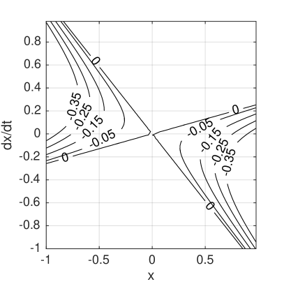
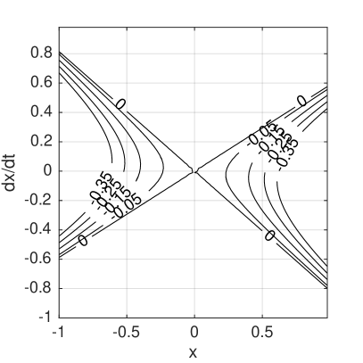
Figure 1: Cones for the mass-spring-damper system for $c=4$ (left) and $c=8$ (right).

$\lrcorner$

$p$-dominance is a generalization of the classical property of exponential stability, which corresponds to $p=0$: all modes are transient and the asymptotic behavior is $0$-dimensional. In contrast, for $p>0$, the property of $p$-dominance is closely connected to the the classical property of positivity [3, 17, 27]. We recall that a linear system $\dot{x}=Ax$ is positive with respect to a cone $\mathcal{K}\subseteq{\mathbb{R}^{n}}$ if $e^{At}\mathcal{K}\subseteq\mathcal{K}$ for all $t\geq 0$. Strict positivity further requires that the system maps any nonzero vector of the boundary of $\mathcal{K}$ into the interior of the cone, for $t>0$.

Proposition 2

For any $0<p<n$, a $p$-dominant system is strictly positive with respect to the cone

$$\mathcal{K}:=\{x\in{\mathbb{R}^{n}}\,|\,x^{T}Px\leq 0\}$$ (2)

where $P$ is any solution to (1).   $\lrcorner$

Proof:

We have to prove that any vector on the boundary of the cone $V(x):=x^{T}Px=0$ is mapped in the cone. Clearly, $\dot{V}(x)=x^{T}(A^{T}P+PA)x<-2\lambda x^{T}Px=0$, which shows the invariance of $\mathcal{K}$. It also shows that any nonzero vector on the boundary is mapped into the interior of $\mathcal{K}$, for $t>0$. ∎

For $p=1$, (1) expresses the contraction of an ellipsoidal cone. The $1$-dimensional dominant subspace is spanned by the Perron-Frobenius eigenvector. For $p>1$, $p$-dominance is also a positivity property with respect to higher order cones [9, 21, 22, 18].

The reader will notice that there is an important distinction between positivity in the sense of Proposition 2 and dominance in the sense of Definition 1. For $p>0$, any dominant system is strictly positive but the converse is not true. This is due to the extra requirement of a nonnegative dissipation rate $\lambda\geq 0$ in the definition of $p$-dominance. The difference is significant because if affects the type of contraction associated to each property. From Proposition 1, $p$-dominance is a form of horizontal contraction in the sense of [7]: the vector space is splitted into a vertical space of dimension $p$ and a horizontal space of dimension $n-p$; contraction is imposed in the horizontal space only. This property requires a nonnegative dissipation rate $\lambda\geq 0$. In contrast, positivity is only a form of projective contraction, which does not require a nonnegative dissipation rate. For $p=1$ the projective contraction is captured by the contraction of the Hilbert metric [3, 14, 2]. The next proposition provides a projective contraction measure for a general $p$.

Proposition 3

For any given $p$-dominant system of dimension $n$, there exist positive semidefinite matrices $P_{u}$ and $P_{s}$ of rank $p$ and $n-p$ respectively such that, given $|x|_{u}:=\sqrt{x^{T}P_{u}x}$ and $|x|_{s}:=\sqrt{x^{T}P_{s}x}$, the ratio $|x(t)|_{s}/|x(t)|_{u}$ is exponentially decreasing along any trajectory $x(\cdot)$ of the system from $|x(0)|_{u}\neq 0$.   $\lrcorner$

Proof:

By Proposition 1, $A+\lambda I$ has $p$ unstable eigenvalues and $n-p$ stable eigenvalues. Thus, there exist matrices $P_{u}$ and $P_{s}$ of rank $p$ and $n-p$ respectively, and a small $\varepsilon>0$, such that $A^{T}P_{u}+P_{u}A\geq(-2\lambda+\varepsilon)P_{u}$ and $A^{T}P_{s}+P_{s}A\leq(-2\lambda-\varepsilon)P_{s}$ Define $U(x)=x^{T}P_{u}x$ and $S(x)=x^{T}P_{s}x$. Then, by comparison theorem, along any trajectory of the system we have $U(x(t))\geq e^{(-2\lambda+\varepsilon)t}U(x(0))$ and $S(x(t))\leq e^{(-2\lambda-\varepsilon)t}S(x(0))$. It follows that

$$S(x(t))/U(x(t))\leq e^{-2\varepsilon t}S(x(0))/U(x0))$$ (3)

which guarantees that the ratio $|x(t)|_{s}/|x(t)|_{u}$ is strictly decreasing and converges to zero as $t\to\infty$. ∎

III $p$-dissipativity

The internal property of $p$-dominance is captured by the matrix inequality (1) which enforces a conic constraint between the state of the system and its derivative of the form

$$\left[\begin{array}[]{c}\!\!\dot{x}\!\!\\ \!\!x\!\!\end{array}\right]^{T}\!\left[\begin{array}[]{cc}0&P\\ P&2\lambda P+\varepsilon I\end{array}\right]\left[\begin{array}[]{c}\!\!\dot{x}\!\!\\ \!\!x\!\!\end{array}\right]\leq 0$$ (4)

where $P$ is a matrix with inertia $(p,0,n-p)$ and $\varepsilon>0$. A system is $p$-dominant if the linear relationship between $\dot{x}$ and $x$ satisfy (4).

Dissipativity theory extends $p$-dominance to open systems by augmenting the internal dissipation inequality with an external supply. The external property of $p$-dissipativity is captured by a conic constraint between the state of the system $x$, its derivative $\dot{x}$, and the external variables $y$ and $u$ of the form

$$\left[\begin{array}[]{c}\!\!\!\dot{x}\!\!\!\\ \!\!\!x\!\!\!\end{array}\right]^{T}\!\!\left[\begin{array}[]{cc}0&P\\ P&2\lambda P+\varepsilon I\end{array}\right]\!\left[\begin{array}[]{c}\!\!\!\dot{x}\!\!\!\\ \!\!\!x\!\!\!\end{array}\right]\leq\left[\begin{array}[]{c}\!\!\!y\!\!\!\\ \!\!\!u\!\!\!\end{array}\right]^{T}\!\!\left[\begin{array}[]{cc}\!Q\!&\!L\!\\ \!L^{T}\!&\!R\!\end{array}\right]\!\left[\begin{array}[]{c}\!\!\!y\!\!\!\\ \!\!\!u\!\!\!\end{array}\right]$$ (5)

where $P$ is a matrix with inertia $(p,0,n-p)$, $\lambda\geq 0$, $L,Q,R$ are matrices of suitable dimension, and $\varepsilon\geq 0$. The property is strict if $\epsilon>0$. We call supply rate $s(y,u):=y^{T}Qy+y^{T}Lu+u^{T}L^{T}y+u^{T}Ru$ the right-hand side of (5). An open dynamical system is $p$-dissipative with rate $\lambda$ if its dynamics $\dot{x}=Ax+Bu$, $y=Cx+Du$ satisfy (5) for all $x$ and $u$.

$p$-dissipativity has a simple characterization in terms of matrix inequalities.

Proposition 4

A linear system $\dot{x}=Ax+Bu$, $y=Cx+Du$ is $p$-dissipative with rate $\lambda$ if and only if there exist a symmetric matrix $P$ with inertia $(p,0,n-p)$ such that

$$\left[\begin{smallmatrix}\!A^{T}\!P+PA+2\lambda P-C^{T}\!QC+\varepsilon I\!&\!PB-C^{T}\!L-C^{T}\!QD\!\\ \!B^{T}P-L^{T}C-D^{T}QC\!&\!-D^{T}QD-L^{T}D-D^{T}L-R\!\end{smallmatrix}\right]\leq 0\,.$$ (6)

$\lrcorner$

Proof:

Just replace $\dot{x}=Ax+Bu$ and $y=Cx+Du$ in (5) and rearrange. [$\Leftarrow$] Multiply (6) by $[x^{T}\,u^{T}]$ on the left, and by $[x^{T}\,u^{T}]^{T}$ on the right. Then we get $\dot{x}^{T}Px+x^{T}P\dot{x}+2\lambda x^{T}Px<s(y,u)$ as desired. ∎

An interconnection theorem can be easily derived.

Proposition 5

Let $\Sigma_{1}$ and $\Sigma_{2}$ $p_{1}$-dissipative and $p_{2}$-dissipative systems respectively, with uniform rate $\lambda$ and with supply rate

$$s_{i}(y_{i},u_{i})=\left[\begin{array}[]{c}\!\!y\!\!\\ \!\!u\!\!\end{array}\right]^{T}\!\left[\begin{array}[]{cc}Q_{i}&L_{i}\\ L_{i}^{T}&R_{i}\end{array}\right]\left[\begin{array}[]{c}\!\!y\!\!\\ \!\!u\!\!\end{array}\right]$$ (7)

for $i\in\{1,2\}$. The closed-loop system given by negative feedback interconnection

$$u_{1}=-y_{2}+v_{1}\qquad u_{2}=y_{1}+v_{2}$$ (8)

is $(p_{1}+p_{2})$-dissipative with rate $\lambda$ from $v=(v_{1},v_{2})$ to $y=(y_{1},y_{2})$ with supply rate

$$s(y,v)=\left[\begin{array}[]{c}\!\!\!y\!\!\!\\ \!\!\!v\!\!\!\end{array}\right]^{\!T}\!\!{\footnotesize\left[\begin{array}[]{cc|cc}Q_{1}+R_{2}&-L_{1}+L_{2}^{T}&L_{1}&R_{2}\\ -L_{1}^{T}+L_{2}&Q_{2}+R_{1}&-R_{1}&L_{2}\\ \hline\cr L_{1}^{T}&-R_{1}&R_{1}&0\\ R_{2}&L_{2}^{T}&0&R_{2}\end{array}\right]\!}\!\left[\begin{array}[]{c}\!\!\!y\!\!\!\\ \!\!\!v\!\!\!\end{array}\right].$$ (9)

The closed loop is $(p_{1}+p_{2})$-dominant with rate $\lambda$ if

$$\left[\begin{array}[]{cc}Q_{1}+R_{2}&-L_{1}+L_{2}^{T}\\ -L_{1}^{T}+L_{2}&Q_{2}+R_{1}\end{array}\right]\leq 0\ .\vspace{-3mm}$$ (10)

$\lrcorner$

Proof:

By standard steps on interconnection of dissipative systems. Define $P:=\left[\begin{smallmatrix}P_{1}&0\\ 0&P_{2}\end{smallmatrix}\right]$ which, by construction, has inertia $(p_{1}+p_{2},0,n_{1}+n_{2}-p_{1}-p_{2})$, where $n_{i}$ is the dimension of the state of system $i\in\{1,2\}$. Then, a simple computation shows that the closed-loop system given by (8), satisfies (5) from $v$ to $y$ with supply rate (9). Furthermore, denote by $S$ the left-hand side of (10) and take $v=0$. Then, using the aggregate state $x=(x_{1},x_{2})$, (10) guarantees $p$-monotonicity since

$$\left[\begin{array}[]{c}\!\!\!\dot{x}\!\!\!\\ \!\!\!x\!\!\!\end{array}\right]^{T}\!\!\!\left[\begin{smallmatrix}0&P\\ P&\,2\lambda P+\varepsilon I\end{smallmatrix}\right]\!\left[\begin{array}[]{c}\!\!\!\dot{x}\!\!\!\\ \!\!\!x\!\!\!\end{array}\right]\leq\left[\begin{array}[]{c}\!\!\!y_{1}\!\!\!\\ \!\!\!y_{2}\!\!\!\end{array}\right]^{T}\!\!\!S\left[\begin{array}[]{c}\!\!\!y_{1}\!\!\!\\ \!\!\!y_{2}\!\!\!\end{array}\right]\leq 0\ .\vspace{-5mm}$$

∎

For $p_{1}=p_{2}=0$ and $\lambda=0$ the proposition reduces to the standard interconnection theorem for dissipative systems, [29]. Like classical dissipativity is related to the internal property of stability, $p$-dissipativity is tightly related to the internal property of $p$-dominance. Thus, for uniform rate $\lambda$, Proposition 5 provides interconnection conditions that lead to $p$-dominant closed loop systems.

Example 2

We say that a system is $p$-passive with rate $\lambda$ when the dissipation inequality (5) is satisfied with supply rate

$$s(y,u)=\left[\begin{array}[]{c}\!\!y\!\!\\ \!\!u\!\!\end{array}\right]^{T}\!\left[\begin{array}[]{cc}0&I\\ I&0\end{array}\right]\left[\begin{array}[]{c}\!\!y\!\!\\ \!\!u\!\!\end{array}\right]\ .$$ (11)

For $D=0$, taking $\varepsilon=0$ for simplicity, (6) reduces to

$$\left\{\begin{array}[]{rcl}A^{T}P+PA&\leq&-2\lambda P\\ PB&=&C^{T}\ .\end{array}\right.$$ (12)

For the open mass-spring system $\dot{x}=\left[\begin{smallmatrix}0&1\\ -1&-8\end{smallmatrix}\right]x+\left[\begin{smallmatrix}0\\ 1\end{smallmatrix}\right]u$, $y=\left[\begin{smallmatrix}0&1\end{smallmatrix}\right]x$, the matrix $P=\left[\begin{smallmatrix}-1&0\\ 0&1\end{smallmatrix}\right]$ satisfies (12) with $\lambda=1.2679$, which gives $1$-passivity from $u$ to $y$. Proposition 5 guarantees that the negative feedback interconnection $u=-ky+v$ is $1$-passive system with rate $\lambda$, for any gain $k\geq 0$. Indeed, the closed-loop system is $1$-dominant for any $k\geq 0$.

A generalized small gain theorem can also be illustrated. We say that a system has $p$-gain $\gamma$ from $u$ to $y$ with rate $\lambda$ when the dissipation inequality (5) is satisfied with supply rate

$$s(y,u)=\left[\begin{array}[]{c}\!\!y\!\!\\ \!\!u\!\!\end{array}\right]^{T}\!\left[\begin{array}[]{cc}-I&0\\ 0&\gamma^{2}I\end{array}\right]\left[\begin{array}[]{c}\!\!y\!\!\\ \!\!u\!\!\end{array}\right]\ .$$ (13)

For the open mass-spring system, the matrix $P$ above satisfies (5) with $L=-I$, $Q=0$ and $R=\gamma^{2}I$ for $\gamma=0.3$. Thus, Proposition 5 guarantees that the closed loop given by the feedback interconnection $u=\pm ky$ is $1$-dominant for any $-3.3<k<3.3$.

The resulting internal dominance is the analog of the resulting stability in classical applications of the passivity theorem and of the small gain theorem [23, 26].   $\lrcorner$

IV Differential analysis and $p$-dominance

$p$-dominance and $p$-dissipativity are not limited to linear systems. In nonlinear analysis it makes sense to study these properties infinitesimally or differentially, see e.g. [6]. In what follows we will see how $p$-dominance of the system linearization restricts the asymptotic behavior of the nonlinear system.

The nonlinear system $\dot{x}=f(x)$ ($f$ smooth, $x\in{\mathbb{R}^{n}}$) is (differentially) $p$-dominant with rate $\lambda\geq 0$ and constant storage $P=P^{T}$ if the prolonged system [4]

$$\dot{x}=f(x)\qquad\dot{\delta x}=\partial f(x)\delta x$$ (14)

satisfies the conic constraint

$$\left[\begin{array}[]{c}\!\!\dot{\delta x}\!\!\\ \!\!\delta x\!\!\end{array}\right]^{T}\!\left[\begin{array}[]{cc}0&P\\ P&2\lambda P+\varepsilon I\end{array}\right]\left[\begin{array}[]{c}\!\!\dot{\delta x}\!\!\\ \!\!\delta x\!\!\end{array}\right]\leq 0$$ (15)

for every $\delta x\in{\mathbb{R}^{n}}$, where $P$ is a matrix with inertia $(p,0,n-p)$ and $\varepsilon\geq 0$. The property is strict if $\epsilon>0$. From (15), the reader will recognize that differential dominance is just dominance of the linearized dynamics. In this paper, we only consider the case of a constant matrix $P$, but generalizations might be considered.

Differential dominance for $p=0$ is another synonym of differential stability, or contraction, or convergence [16, 19, 20, 7]. The trajectories of the nonlinear system converge exponentially towards each other. In fact, (15) reduces to the inequality

$$\partial f(x)^{T}P+P\partial f(x)\leq-\epsilon I\qquad\forall x\in{\mathbb{R}^{n}}$$ (16)

where $P$ is a positive definite matrix. This is a typical condition for contraction with respect to a constant (Riemannian) metric $P$ [7]. The following proposition is a straightforward consequence of (16).

Proposition 6

If $\dot{x}=f(x)$ is strictly $0$-dominant, then all solutions exponentially converge to a unique fixed point.   $\lrcorner$

Proof:

Denote by $\psi^{t}(x)$ the semiflow of $\dot{x}=f(x)$, characterizing the trajectory of the system at time $t$ from the initial condition $x$ at initial time zero. Then, contraction guarantees that the distance $d_{P}(x_{1},x_{2}):=((x_{1}-x_{2})^{T}P(x_{1}-x_{2}))^{1/2}$ is exponentially decreasing along any pair of trajectories $x_{1}(\cdot),x_{2}(\cdot)$, [19, 7]. Indeed, for any $t>0$, $\psi^{t}(\cdot)$ is a contraction mapping on ${\mathbb{R}^{n}}$ with respect to $d_{P}$. By Banach fixed point theorem $\psi^{t}(\cdot)$ admits a unique fixed-point $x^{*}$ in ${\mathbb{R}^{n}}$. By contraction every trajectory converges to $x^{*}$ exponentially. ∎

For $p=1$, differential dominance is closely related to differential positivity with respect to a constant ellipsoidal cone $\mathcal{K}\subseteq{\mathbb{R}^{n}}$, [8]. A straightforward adaptation of Proposition 2 shows that the linearized trajectories of a differentially $1$-dominant system map the boundary of the cone $\mathcal{K}:=\{\delta x\in{\mathbb{R}^{n}}\,|\,\delta x^{T}P\delta x\leq 0\}$ into its interior, as required by strict differential positivity. We observe that $\mathcal{K}$ is the union of two pointed convex cones $\mathcal{K}=\mathcal{K}_{+}\cup\mathcal{K}_{-}$ such that $\mathcal{K}_{+}\cap\mathcal{K}_{-}=\{0\}$. Then, differential 1-dominance also guarantees strict differential positivity with respect to $\mathcal{K}_{+}$ (and to $\mathcal{K}_{-}$), which follows from strict differential positivity with respect to $\mathcal{K}$ and from the fact that the contact point between $\mathcal{K}_{+}$ and $\mathcal{K}_{-}$ is $\delta x=0$, which is a fixed point of the linearization. Thus, differential $1$-dominance guarantees strict differential positivity with respect to a constant solid, pointed, convex cone in ${\mathbb{R}^{n}}$, which leads to the following result.

Proposition 7

If $\dot{x}=f(x)$ is strictly $1$-dominant, then all bounded solutions exponentially converge to some fixed point.   $\lrcorner$

Proof:

The details of the proof are omitted but the the proof closely follows the arguments in [8, Corollary 5]. ∎

Differential $1$-dominance also closely relates to monotonicity [24, 12, 1, 13] with respect to the partial order $\preceq$ induced by $\mathcal{K}_{+}$: $x\preceq y$ iff $y-x\in\mathcal{K}_{+}$. In fact, differential $1$-dominance guarantees that any pair of trajectories $x_{1}(\cdot)$, $x_{2}(\cdot)$ of the nonlinear system from ordered initial conditions $x_{1}(0)\preceq x_{2}(0)$ satisfy $x_{1}(t)\preceq x_{2}(t)$ for all $t\geq 0$, as required by classical monotonicity (a direct consequence of the relation with differential positivity [8]). In this sense, Proposition 7 is the counterpart of the well know property that almost every bounded trajectory of a monotone system converges to a fixed point [11, 24]. The fact that the property holds for all trajectories in differentially 1-dominant systems follows from the nonnegative dissipation rate $\lambda\geq 0$, which is not necessary for monotonicity.

For $p=2$, differential dominance closely relates to the notion of monotonicity with respect rank-$2$ cones of [21, 25], see [21, Equations (7) and (8)].

Proposition 8

If $\dot{x}=f(x)$ is strictly $2$-dominant, then all bounded solutions whose $\omega$-limit set does not contain an equilibrium point exponentially converge to a closed orbit.   $\lrcorner$

Proof:

The details of the proof are left to an extended version of this paper but the the proof closely follows the arguments in [21, Theorem 1]. ∎

Proposition 8 shows that differentially $2$-dominant systems enjoy properties akin to the Poincare-Bendixson theory of planar systems.

V Differential analysis and $p$-dissipativity

In analogy with the previous section, we use the prolonged system to define $p$-dissipativity in a nonlinear setting. For simplicity we will consider systems of the form $\dot{x}=f(x)+Bu$, $y=Cx$ ($f$ is smooth, $x\in{\mathbb{R}^{n}}$, $u\in{\mathbb{R}}^{m}$), whose prolonged system [4] is given by

$$\left\{\begin{array}[]{rcl}\dot{x}&=&f(x)+Bu\\ y&=&Cx\end{array}\right.\qquad\left\{\begin{array}[]{rcl}\dot{\delta x}&=&\partial f(x)\delta x+B\delta u\\ \delta y&=&C\delta x\ .\end{array}\right.$$ (17)

A nonlinear system is differentially $p$-dissipative with rate $\lambda\geq 0$ if its prolonged system satisfies the conic constraint

$$\left[\begin{array}[]{c}\!\!\!\dot{\delta x}\!\!\!\\ \!\!\!\delta x\!\!\!\end{array}\right]^{T}\!\!\left[\begin{array}[]{cc}\!0\!&\!P\!\\ \!P\!&\!2\lambda P\!+\!\varepsilon I\!\end{array}\right]\!\left[\begin{array}[]{c}\!\!\!\dot{\delta x}\!\!\!\\ \!\!\!\delta x\!\!\!\end{array}\right]\leq\left[\begin{array}[]{c}\!\!\!\delta y\!\!\!\\ \!\!\!\delta u\!\!\!\end{array}\right]^{T}\!\!\left[\begin{array}[]{cc}\!Q\!&\!L\!\\ \!L^{T}\!&\!R\!\end{array}\right]\!\left[\begin{array}[]{c}\!\!\!\delta y\!\!\!\\ \!\!\!\delta u\!\!\!\end{array}\right]$$ (18)

for every $\delta x\in{\mathbb{R}^{n}}$ and every $\delta u\in{\mathbb{R}}^{m}$, where $P$ is a matrix with inertia $(p,0,n-p)$, $L,Q,R$ are matrices of suitable dimension, and $\varepsilon>0$.

The following interconnection result easily follows.

Proposition 9

Let $\Sigma_{1}$ and $\Sigma_{2}$ differentially $p_{1}$-dissipative and differentially $p_{2}$-dissipative respectively, with uniform rate $\lambda$ and with differential supply rate

$$s_{i}(\delta y_{i},\delta u_{i})=\left[\begin{array}[]{c}\!\!\delta y\!\!\\ \!\!\delta u\!\!\end{array}\right]^{T}\!\left[\begin{array}[]{cc}Q_{i}&L_{i}\\ L_{i}^{T}&R_{i}\end{array}\right]\left[\begin{array}[]{c}\!\!\delta y\!\!\\ \!\!\delta u\!\!\end{array}\right]$$ (19)

for $i\in\{1,2\}$. The closed-loop system given by negative feedback interconnection (8) is differentially $(p_{1}+p_{2})$-dissipative with rate $\lambda$ from $v=(v_{1},v_{2})$ to $y=(y_{1},y_{2})$ with differential supply rate with supply rate

$$s(y,v)\!=\!\left[\begin{array}[]{c}\!\!\!\delta y\!\!\!\\ \!\!\!\delta v\!\!\!\end{array}\right]^{\!T}\!\!{\footnotesize\left[\begin{array}[]{cc|cc}Q_{1}+R_{2}&-L_{1}+L_{2}^{T}&L_{1}&R_{2}\\ -L_{1}^{T}+L_{2}&Q_{2}+R_{1}&-R_{1}&L_{2}\\ \hline\cr L_{1}^{T}&-R_{1}&R_{1}&0\\ R_{2}&L_{2}^{T}&0&R_{2}\end{array}\right]\!}\!\left[\begin{array}[]{c}\!\!\!\delta y\!\!\!\\ \!\!\!\delta v\!\!\!\end{array}\right].$$ (20)

The closed loop is differentially $(p_{1}+p_{2})$-dominant if (10) holds.   $\lrcorner$

Proposition 9 provides an interconnection result for differential $p$-dominance. For example, under the assumptions of the proposition, the closed loop of a $1$-dominant system (typically a monotone system) with a $0$-dominant system (typically a contractive system) is necessarily $1$-dominant. In a similar way, the closed loop of two $1$-dominant systems leads to $2$-dominance. In this sense, Proposition 9 provides an interconnection mechanism to generate periodic behavior ($2$-dominance) from the interconnection of multi-stable components ($1$-dominance).

Remark 1

Both $p$-dominance and $p$-dissipativity can be tested algorithmically via simple relaxations. From (14) and (15) $p$-dominance requires that

$$\partial f(x)^{T}P+P\partial f(x)<-2\lambda P\qquad\forall x\in{\mathbb{R}^{n}}\ .$$ (21)

From (17) and (18) differential $p$-dissipativity requires that

$${\small\left[\begin{array}[]{cc}\!\!\!\partial\!f(x)^{T}\!P\!+\!P\partial\!f(x)\!+\!2\lambda P\!-\!C^{T}\!QC\!+\!\varepsilon I\!&\!PB\!-\!C^{T}\!L\!\!\!\\ \!\!B^{T}\!P\!-\!L^{T}C\!\!&\!\!-R\!\!\!\end{array}\right]}\!\leq\!0\,.$$ (22)

Let $\mathcal{A}:=\{A_{1},\dots,A_{N}\}$ be a family of matrices such that $\partial f(x)\in\mathit{ConvexHull}(\mathcal{A})$ for all $x$. Then, by construction, any (uniform) solution $P$ to

$$A_{i}^{T}P+PA_{i}<-2\lambda P\qquad 1\leq i\leq N$$ (23)

is a solution to (21). Also, any (uniform) solution $P$ to

$${\small\left[\begin{array}[]{cc}\!\!\!A_{i}^{T}P+PA_{i}+2\lambda P-C^{T}QC+\varepsilon I\!\!&\!\!PB-C^{T}L\!\!\!\\ \!\!B^{T}P-L^{T}C\!\!&\!\!-R\!\!\!\end{array}\right]}\leq 0$$ (24)

for $1\leq i\leq N$ is a solution to (22).

We recall that if $\lambda$ is chosen in such a way that each $A_{i}+\lambda I$ has exactly $p$ unstable eigenvalues, then $P$ necessarily have inertia $(p,0,n-p)$.   $\lrcorner$

Example 3

We revisit Examples 1 and 2 by replacing the linear spring with a nonlinear active component $\phi(x_{1})$

$$\left\{\begin{array}[]{rcl}\dot{x_{1}}&=&x_{2}\\ \dot{x_{2}}&=&\phi(x_{1})-8x_{2}+u\ .\\ \end{array}\right.$$ (25)

A strictly monotone nonlinear spring $-2\leq\partial\phi(x_{1})<-1/2$ makes the system $0$-dominant with rate $\lambda=0$. For instance, the linearization reads $\dot{\delta x}=A(x)\delta x+Bu$ with

$$A(x):=\left[\begin{array}[]{cc}0&1\\ \partial\phi(x_{1})&-8\end{array}\right]\,,\ B:=\left[\begin{array}[]{c}0\\ 1\end{array}\right]\ ,$$ (26)

and the matrix $P:=\left[\begin{smallmatrix}1&0.5\\ 0.5&1\end{smallmatrix}\right]$ satisfies the inequality $A(x)^{T}P+PA(x)<-\lambda P$ uniformly in $x$ for $\lambda=0$. By Proposition 6 the trajectories of the system exponentially converge to the unique fixed point of the system.

A non-monotone spring $-3\leq\partial\phi(x_{1})<1$ shifts the eigenvalues of $A(x)$ to the right-half complex plane. $0$-dominance can no longer hold. However, the matrix $P:=\left[\begin{smallmatrix}-1&0\\ 0&1\end{smallmatrix}\right]$ satisfies $A(x)^{T}P+PA(x)<-\lambda P$ uniformly in $x$ for $\lambda=1$, which makes the system $1$-dominant. The system is differentially $1$-passive with rate $\lambda$ from $u$ to $y=Cx=x_{2}$ since $[\,0\ 1\,]^{T}=:C^{T}\!=PB$. Propositions 7 and 9 guarantee that the closed loop system given by $u=-ky$ is $1$-dominant for any $k\geq 0$. All trajectories of the closed loop converge to a fixed point.

Different outputs can also be considered. For example, again for $-3\leq\partial\phi(x_{1})<1$, the dissipation inequality is satisfied uniformly in $x$ by the matrix $P:=\left[\begin{smallmatrix}-2&1\\ 1&2\end{smallmatrix}\right]$ which makes (25) differentially $1$-passive from $u$ to $y=Cx=x_{1}+2x_{2}$ since $[\,1\ 2\,]^{T}=:C^{T}\!=PB$. By Proposition 9, the negative feedback interconnection of two mass-spring-damper systems is differentially $2$-passive with rate $\lambda=1$. The $4$-dimensional system is $2$-dominant and, with some extra work, it can be proven that all solutions converge either to the unstable equilibrium or to a limit cycle, as illustrated by the simulation in Figure 2, where $\phi(x_{1})=x_{1}-\frac{1}{3}\min(x_{1}^{2},4)x_{1}$.

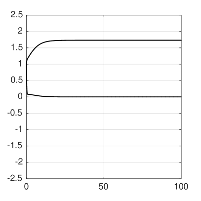
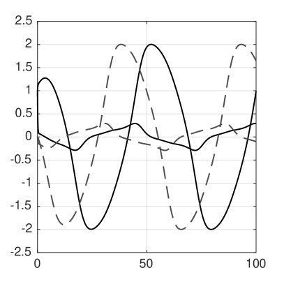
Figure 2: Left: position and velocity of the single nonlinear mass spring damper system with nonlinear spring $\phi(x_{1})=x_{1}-\frac{1}{3}\min(x_{1}^{2},4)x_{1}$. Unforced behavior (stable fixed point) from the initial condition $x_{1}=1$, $x_{2}=1$. Right: positions variables of the closed loop of two mass spring damper systems with nonlinear spring $\phi(x_{1})$ in feedback interconnection from the input $u$ to the output $y=x_{1}+2x_{2}$. Trajectories converge to a limit cycle.

$\lrcorner$

VI Conclusions

We introduced the notions of $p$-dominance and $p$-dissipativity both in the linear and nonlinear settings. They provide a conceptual and algorithmic framework for the analysis of multi-stable and periodic behaviors. Interconnection theorems are provided which extend classical dissipativity theory with indefinite storages. The example illustrates the potential of the approach.

The paper only exposes the basic ideas of the proposed approach. Future research directions will include a frequency domain characterization for $p$-dominance and $p$-dissipativity. In the nonlinear setting it is relevant to extend the framework to the case of non-constant matrix $P(x)$ and rate $\lambda(x)$, following the lead of differential stability [7] and differential positivity [8, 5]. Finally, the interconnection theorems in the paper only consider quadratic supplies and storages but the concept of $p$-dissipativity is of course more general.

References

• [1] D.ย Angeli and E.D. Sontag. Monotone control systems. IEEE Transactions on Automatic Control, 48(10):1684 โ€“ 1698, 2003.
• [2] S.ย Bonnabel, A.ย Astolfi, and R.ย Sepulchre. Contraction and observer design on cones. In Proceedings of 50th IEEE Conference on Decision and Control and European Control Conference, pages 7147โ€“7151, 2011.
• [3] P.J. Bushell. Hilbertโ€™s metric and positive contraction mappings in a Banach space. Archive for Rational Mechanics and Analysis, 52(4):330โ€“338, 1973.
• [4] P.E. Crouch and A.J. vanย der Schaft. Variational and Hamiltonian control systems. Lecture notes in control and information sciences. Springer, 1987.
• [5] Fย Forni. Differential positivity on compact sets. In 54th IEEE Conference on Decision and Control, pages 6355โ€“6360, 2015.
• [6] F.ย Forni and R.ย Sepulchre. Differential analysis of nonlinear systems: Revisiting the pendulum example. In 53rd IEEE Conference on Decision and Control, pages 3848โ€“3859, 2014.
• [7] F.ย Forni and R.ย Sepulchre. A differential Lyapunov framework for contraction analysis. IEEE Transactions on Automatic Control, 59(3):614โ€“628, 2014.
• [8] F.ย Forni and R.ย Sepulchre. Differentially positive systems. IEEE Transactions on Automatic Control, 61(2):346โ€“359, 2016.
• [9] G.ย Fusco and W.M. Oliva. A Perron theorem for the existence of invariant subspaces. Annali di Matematica Pura ed Applicata, 160(1):63โ€“76, 1991.
• [10] G.T. Gilbert. Positive definite matrices and Sylvesterโ€™s criterion. The American Mathematical Monthly, 98(1):44โ€“46, 1991.
• [11] M.W. Hirsch. Stability and convergence in strongly monotone dynamical systems. Journal fรผr die reine und angewandte Mathematik, 383:1โ€“53, 1988.
• [12] M.W. Hirsch and H.L. Smith. Competitive and cooperative systems: A mini-review. In L.ย Benvenuti, A.ย Santis, and L.ย Farina, editors, Positive Systems, volume 294 of Lecture Notes in Control and Information Science, pages 183โ€“190. Springer Berlin Heidelberg, 2003.
• [13] M.W. Hirsch and H.L. Smith. Monotone dynamical systems. In P.ย Drabek A.ย Canada and A.ย Fonda, editors, Handbook of Differential Equations: Ordinary Differential Equations, volumeย 2, pages 239 โ€“ 357. North-Holland, 2006.
• [14] E.ย Kohlberg and J.W. Pratt. The contraction mapping approach to the Perron-Frobenius theory: Why Hilbertโ€™s metric? Mathematics of Operations Research, 7(2):pp. 198โ€“210, 1982.
• [15] J.ย Lรถfberg. Yalmip : a toolbox for modeling and optimization in matlab. In Computer Aided Control Systems Design, 2004 IEEE International Symposium on, pages 284โ€“289, 2004.
• [16] W.ย Lohmiller and J.E. Slotine. On contraction analysis for non-linear systems. Automatica, 34(6):683โ€“696, June 1998.
• [17] D.G. Luenberger. Introduction to Dynamic Systems: Theory, Models, and Applications. Wiley, 1 edition, 1979.
• [18] C.ย Mostajeran and R.ย Sepulchre. Differential positivity with respect to cones of rank k. In 20th IFAC World Congress, 2017.
• [19] A.ย Pavlov, N.ย vanย de Wouw, and H.ย Nijmeijer. Uniform Output Regulation of Nonlinear Systems: A Convergent Dynamics Approach. Systems & Control: Foundations & Applications. Birkhรคuser, 2005.
• [20] G.ย Russo, M.ย Diย Bernardo, and E.D. Sontag. Global entrainment of transcriptional systems to periodic inputs. PLoS Computational Biology, 6(4):e1000739, 04 2010.
• [21] L.A. Sanchez. Cones of rank 2 and the Poincarรฉโ€“Bendixson property for a new class of monotone systems. Journal of Differential Equations, 246(5):1978 โ€“ 1990, 2009.
• [22] L.A. Sanchez. Existence of periodic orbits for high-dimensional autonomous systems. Journal of Mathematical Analysis and Applications, 363(2):409 โ€“ 418, 2010.
• [23] R.ย Sepulchre, M.ย Jankovic, and P.ย Kokotovic. Constructive nonlinear Control. Springer Verlag, 1997.
• [24] H.L. Smith. Monotone Dynamical Systems: An Introduction to the Theory of Competitive and Cooperative Systems, volumeย 41 of Mathematical Surveys and Monographs. American Mathematical Society, 1995.
• [25] R.A. Smith. Orbital stability for ordinary differential equations. Journal of Differential Equations, 69(2):265 โ€“ 287, 1987.
• [26] A.J. vanย der Schaft. $L_{2}$-Gain and Passivity in Nonlinear Control. Springer-Verlag New York, Inc., Secaucus, N.J., USA, second edition, 1999.
• [27] J.S. Vandergraft. Spectral properties of matrices which have invariant cones. SIAM Journal on Applied Mathematics, 16(6):pp. 1208โ€“1222, 1968.
• [28] J.C. Willems. Dissipative dynamical systems part I: General theory. Archive for Rational Mechanics and Analysis, 45:321โ€“351, 1972.
• [29] J.C. Willems. Dissipative dynamical systems part II: Linear systems with quadratic supply rates. Archive for Rational Mechanics and Analysis, 45:352โ€“393, 1972.