The bimodal Ising spin glass in dimension two : the anomalous dimension $\eta$

Abstract

Direct measurements of the spin glass correlation function $G(R)$ for Gaussian and bimodal Ising spin glasses in dimension two have been carried out in the temperature region $T\sim 1$. In the Gaussian case the data are consistent with the known anomalous dimension value $\eta\equiv 0$. For the bimodal spin glass in this temperature region $T>T^{*}(L)$, well above the crossover $T^{*}(L)$ to the ground state dominated regime, the effective exponent $\eta$ is clearly non-zero and the data are consistent with the estimate $\eta\sim 0.28(4)$ given by McMillan in 1983 from similar measurements. Measurements of the temperature dependence of the Binder cumulant $U_{4}(T,L)$ and the normalized correlation length $\xi(T,L)/L$ for the two models confirms the conclusion that the 2D bimodal model has a non-zero effective $\eta$ both below and above $T^{*}(L)$. The 2D bimodal and Gaussian interaction distribution Ising spin glasses are not in the same Universality class.

I Introduction

The square lattice near neighbor random interaction Ising models are canonical examples of the Edwards-Anderson Ising Spin Glasses (ISG) edwards:75 . Numerous studies of these models have been made over the years, interest being mainly focussed on two versions of this 2D ISG model : the Gaussian model where the random interaction distribution takes up the continuous Gaussian form and the ground state is unique, and the bimodal model where positive or negative interactions ($\pm J$) are randomly distributed, and where the ground state is massively degenerate. It is well established that both these models (and any other 2D ISGs) order only at zero temperature ohzeki:09 . (Temperatures will be quoted in units of $J$).

For any continuous distribution model including the Gaussian the anomalous dimension critical exponent is analytically known to be $\eta\equiv 0$ because the ground state is non-degenerate; accurate and consistent estimates have been made of the correlation length critical exponent $\nu=3.52(2)$ for the Gaussian model hartmann:02 ; carter:02 ; hartmann:02a ; houdayer:04 ; lundow:16 ; fernandez:16 and for other continuous distribution models lundow:17 . The values of other critical exponents, in particular the magnetization exponent $\gamma=(2-\eta)\nu$, follow.

For the discrete interaction bimodal model the ordering process is more complex. It has been established that for finite lattice size $L$ there can be considered to be two regimes separated by a crossover temperature $T^{*}(L)$, a ”ground state plus gap” regime for $T<T^{*}(L)$, and an ”effectively continuous energy level” regime for $T>T^{*}(L)$ jorg:06 . In the infinite-$L$ thermodynamic limit (ThL) $T^{*}$ reaches zero because $T^{*}(L)$ drops with increasing $L$ as $T^{*}(L)\sim 1.1(1)L^{-1/2}$ thomas:11 ; lundow:16 . In the strict ground-state limit $T\equiv 0$ and for finite $L$, the bimodal 2D ISG exponent $\eta$ has been estimated to be $\eta=0.210(23)$ ozeki:90 from transfer-matrix ground-state measurements, $\eta=0.14(1)$ from ground-state spin correlations poulter:05 and $\eta=0.22(1)$ from non-zero-energy droplet probabilities hartmann:08 .

There have been consistent estimates over decades indicating a bimodal ISG effective $\eta\sim 0.20$ in the $T>T^{*}(L)$ regime also. Initial estimates were from direct finite-temperature correlation function measurements: first $\eta=0.4(1)$ morgenstern:80 , and then from more precise data $\eta=0.28(4)$ mcmillan:83 . The latter estimate was qualitatively confirmed by a Monte Carlo renormalization-group measurement which indicated $\eta\sim 0.20$ wang:88 again in what can now be recognized as being the $T>T^{*}(L)$ regime note1 . Later numerical simulation estimates were $\eta\sim 0.20$ houdayer:01 , $\eta\sim 0.138$ katzgraber:05 , $\eta>0.20$ katzgraber:07 , $\eta=0.20(2)$ lundow:16 .

These results strongly suggest an anomalous dimension critical exponent $\eta\sim 0.20$ in both regimes, above and below $T^{*}(L)$ note2 , indicating that the bimodal model in the effectively continuous energy distribution regime $T>T^{*}(L)$ does not have the same effective exponent $\eta$ as the Gaussian model. Recent estimates for the bimodal correlation function exponent are $\nu\sim 5.5$ thomas:11 and $\nu=4.8(3)$ lundow:16 , both significantly higher than the accepted estimate for the Gaussian model. ”Quotient” analyses for the bimodal model fernandez:16 are consistent with the higher value lundow:17 .

Nevertheless, the claim has repeatedly been made that the bimodal model in the $T>T^{*}(L)$ regime is in the same universality class as the Gaussian model, Jörg et al. jorg:06 , Parisen Toldin et al. parisen:10 ; parisen:11 , and Fernandez et al. fernandez:16 . It is thus claimed that in the effectively continuous energy distribution regime $T>T^{*}(L)$ the bimodal anomalous dimension exponent is $\eta=0$ and the bimodal correlation length exponent is $\nu=3.52(2)$. The texts of the articles claiming this Universality do not mention the numerous published measurements showing a non-zero bimodal model $\eta$ value in the $T>T^{*}(L)$ regime.

II Correlation function measurements

In 1983 McMillan mcmillan:83 carried out direct numerical measurements of the ISG correlation function

$$G(R)=\frac{1}{2N}\sum_{i,j}\langle S_{i}S_{j}\rangle^{2}\delta(R_{i,j}-R)$$ (1)

for the 2D bimodal ISG at size $L=96$ as a function of separation $R$ up to $R=16$, for temperatures down to $T=0.89$. As the correlation function is written $G(R,T)\sim\exp[-R/\xi(T)]/R^{\eta}$ this is a fundamental defining measurement for $\eta$. It gives a basic qualitative criterion from which to judge if $\eta$ is zero or not. If $\eta=0$, then each plot of $\ln[G(R,T)]$ against $R$ should be a straight line with a slope proportional to $1/\xi(T)$. If $\eta$ is not zero, then the $\ln[G(R,T)]$ against $R$ plots should curve upwards. By inspection, the lowest temperature plots (where the $\xi(T)$ values are highest) in Ref. mcmillan:83 Fig. 1 can be seen to curve upwards, demonstrating that $\eta$ in the 2D bimodal ISG is not zero. In more detail, fits to the data provide numerical estimates for $\eta$ and for correlation lengths $\xi(T)$. McMillan estimated $\eta=0.28(4)$ and obtained correlation length estimates over a narrow temperature range around $T=1$ mcmillan:83 . As remarked by McMillan, a large number of Monte Carlo update steps ($10^{6}$ in his case) after equilibration are required to achieve stability of the $G(R,T)$ curves.

As far as we are aware this measurement has never been repeated. We have been able to extend the measurements to rather lower temperatures, involving many more update steps, thanks to the improvements in computing technology over the years (McMillan built his own computer). The number of updates in the present study cannot be compared directly with Ref. mcmillan:83 as the update procedures were different. Unfortunately McMillan was killed in an accident in 1985 and the tabulated data corresponding to his Fig. 1 are lost. Agreement is however excellent between the points read off in Ref. mcmillan:83 Fig. 1 by eye and the present data for the same bimodal $G(R,L,T)$.

Data were generated for 2D lattices of linear order $L=16$, $24$, $32$, $48$, $64$, $96$ with periodic boundary conditions. The spin interactions $J_{ij}$ were chosen from a bimodal distribution ($\pm 1$ with equal probability) and from a Gaussian distribution $\mathcal{N}(0,1)$ respectively. During the equilibration phase standard heat-bath updates were combined with the exchange Monte Carlo hukushima:96 and the Houdayer cluster method houdayer:01 on four replicas. We used $75$ temperatures in geometric progression between $0.50\leq\beta\leq 1.50$ and also for $1\leq\beta\leq 3$. The same temperature set was thus used on all lattice sizes. Some $500\ 000$ updates (consisting of a heat-bath update, temperature exchange and cluster flips) were made in the equilibration phase for $L=96$. The spin systems were deemed equilibrated when the estimated specific heat value ($\chi$) only fluctuated in a random fashion between runs. Once equilibrated we used only heat-bath updates to measure $G(R)$ after every update.

III Gaussian interaction ISG

We first show data for the ”simple” 2D Gaussian interaction distribution model where the asymptotic correlation function after a sufficient number of updates has the zero $\eta$ form $\ln[G(R,\beta)]\sim K-R/\xi(\beta)$ with $K\sim-0.7$, at all temperatures studied. Fig. 1 shows as an example data for $L=64$ after $10^{9}$ updates at inverse temperatures from $\beta=0.6$ to $\beta=1.5$. It can be seen that the linear asymptotic expression holds well over the entire range of $R$, except for deviations in the pre-asymptotic regime at very small $R$ ($R=0$ and $R=1$ essentially), and when $R$ approaches $L/2$ closely. In the latter limit even after an infinite number of update steps $G(R)$ must become independent of $R$ because of well known periodic boundary condition effects : correlations with ”ghost” sites such as $[\pm L,0,0]$ add to the direct correlation with the site $[0,0,0]$ talapov:93 .

In Fig. 2 we apply the chi-square test parameter $\chi^{2}=\sum_{R}(G(R)-G_{\mathrm{fit}}(R))^{2}/G_{\mathrm{fit}}(R)$ to fits to the $G(R)$ data, with $R$ from $3$ to $25$ and the three lowest temperatures of Fig. 1. With the appropriate correlation lengths $\xi(\beta)$ fixed and $\eta$ allowed to vary in the fitting procedure, the chi-square goodness of fit is consistently at a minimum for $\eta=0$, the physical value for the Gaussian model, which is a test of the quality of the measured $G(R)$ data.

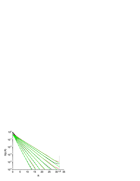
Figure 1: (Color on line) Correlations $G(R)$ as functions of distance $R$ for the $L=64$ Gaussian 2D ISG. Inverse temperatures $\beta=0.8$, $0.9$, $1.0$, $1.1$, $1.2$, $1.3$, $1.4$, $1.5$ from left to right. Green lines : Fits $G(R,\beta)\sim\exp[-R/\xi(\beta)]$

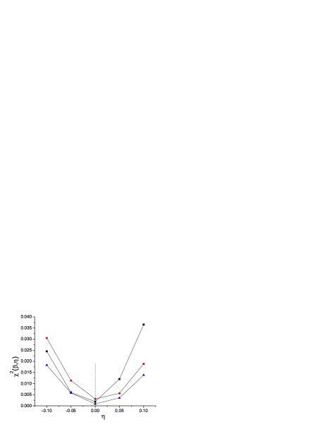
Figure 2: (Color on line) Chi-square fit criterion for fits to the $L=64$ Gaussian 2d ISG $G(R)$ data of Fig. 1 at inverse temperatures $\beta=1.5$ (black squares), $1.4$ (red circles), $1.3$ (blue triangles). Fits with $\xi(\beta)=3.57$, $3.3$ and $2.78$, and $\eta$ from $-0.10$ to $0.10$.

The estimated correlation length $\xi(\beta)$ increases with increasing $\beta$ as expected. The set of measured correlation lengths $\xi(\beta)$ can be compared to the raw simulation data for the second-moment correlation length at similar inverse temperatures which were generated for Ref. lundow:16 , Fig. 3. The temperature dependence of the two sets is very similar. The offset by a factor of about $1.15$ can be ascribed to the fact that two different correlation lengths are being measured; the so-called ”true” correlation length along lattice axes in the present work, and the second-moment correlation length in Ref. lundow:16 . These two lengths and their differences are discussed for the case of the canonical 2D and 3D Ising models in Ref. butera:04 . Neither in the Gaussian case nor in the bimodal case below will we analyse in terms of an effective correlation length exponent $\nu$, as the range of temperatures over which measurements were carried out was small and far from $T=0$ criticality.

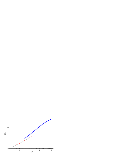
Figure 3: (Color on line)$L=64$ Gaussian 2D ISG. Effective correlation lengths as functions of inverse temperature $\beta$. Second-moment correlation length from the data generated for Ref. lundow:16 : blue triangles. ”True” correlation length, present data, Fig. 1 : red circles.

IV Bimodal interaction ISG

The data for $L=96$ after $10^{10}$ updates for inverse temperatures $\beta=1.1$ to $1.5$ are shown in Fig. 4. Other measurements were made from $\beta=0.6$ to $\beta=1.0$ after $10^{9}$ updates which was sufficient for these higher temperatures. It can be seen by inspection of Figs. 4 and 5 that $\ln[G(R,\beta)]$ against $R$ takes the form of curves and not straight lines, which is a clear qualitative demonstration that for this model in this temperature range $\eta$ is not zero. It can be noted that specific heat data Ref. thomas:11 ; lundow:16 indicate that the ”crossover” temperature for $L=96$ is about $T^{*}(L)\sim 0.12$ so all the present data are well inside the $T>T^{*}(L)$ ”effectively continuous energy level” regime.

In Fig. 6 the same chi-square test procedure as in Fig. 2 is applied to the bimodal $G(R)$ data for the three lowest temperatures of Fig. 5. Here the chi-square goodness of fit is consistently at a minimum for $\eta$ between $0.28$ and $0.30$, which is consistent with the McMillan estimate $\eta=0.28(4)$. A fit with $\eta$ fixed to $0$ can obviously be ruled out.

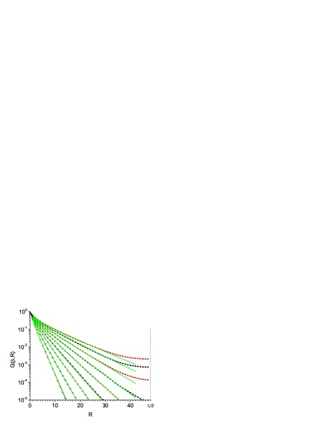
Figure 4: (Color on line) Correlations $G(R)$ as functions of distance $R$ for the $L=96$ bimodal 2D ISG. Inverse temperatures $\beta=0.8$, $0.9$, $1.0$, $1.1$, $1.2$, $1.3$, $1.4$, $1.5$ from left to right. Green curves : fits $G(\beta,R)=K\exp[-R/\xi(\beta)]/R^{0.28}$.

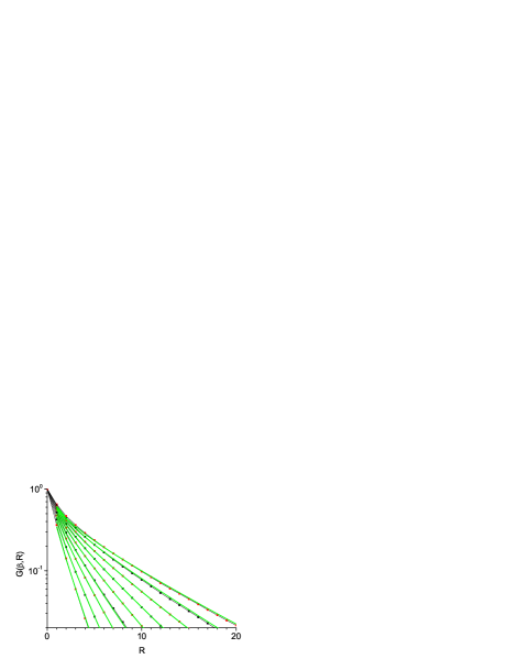
Figure 5: (Color on line) $L=96$ bimodal 2D ISG $G(R)$ small-$R$ region. Data and fits as in Fig. 4

Good fits to all the curves have been obtained using a similar assumption as that made by McMillan, an effective $\eta\sim 0.28$ in this temperature range. In Fig. 7 the effective correlation lengths $\xi(\beta)$ estimated from the fits are compared to the values obtained from the explicit temperature dependence expression, Ref. mcmillan:83 Eq. (5), and to the raw bimodal second-moment correlation lengths from data generated for Ref. lundow:16 . The agreement with McMillan’s empirical Eq. (5) for the true correlation length (from 35 years ago) is almost perfect. The true correlation lengths $\xi_{\mathrm{true}}(\beta)$ from the present work and the second-moment correlation lengths $\xi(\beta)$ for $L=96$ from data generated for Ref. lundow:16 have a qualitatively similar behavior with an offset such that $\xi_{2m}(T)\sim 1.15\,\xi_{\mathrm{true}}(T)$, just as for the equivalent lengths in the Gaussian model Fig. 3.

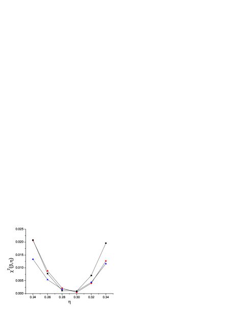
Figure 6: (Color on line) Chi-square fit criterion for fits to the $L=96$ bimodal 2d ISG $G(R)$ data of Fig. 5 at inverse temperatures $\beta=1.5$ (black squares), $1.4$ (red circles), $1.3$ (blue triangles). Fits with $\xi(\beta)=7.35$, $6.3$ and $5.15$, and $\eta$ from $0.24$ to $0.34$.

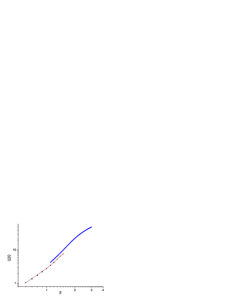
Figure 7: (Color on line) $L=96$ bimodal 2D ISG. Effective correlation lengths as functions of inverse temperature $\beta$. Second-moment correlation length from the data generated for Ref. lundow:16 : blue triangles. ”True” correlation length, present data, Fig. 1 : red circles.

V End points

As discussed in Ref. lundow:17 , for any model (including both Ising and ISG models) the values at criticality of dimensionless parameters such as the Binder cumulant $U_{4}(T,L)$ (in the ISG case $U_{4}=[\langle q^{4}\rangle]/[\langle q^{2}\rangle]^{2}$ with $q$ the ISG order parameter defined as usual by $q=(1/L^{d})\sum_{i}S_{i}^{A}S_{i}^{B}$ where A and B indicate two copies of the same system and the sum is over all sites) and the second-moment correlation length ratio $\xi(T,L)/L$ (see Refs. butera:04 ; katzgraber:05 ) depend only on the critical exponent $\eta$ (see Ref. salas:00 ).

For any $[T_{c}=0,\eta\equiv 0]$ model such as the 2D Gaussian ISG, $U_{4}(T,L)$ as a function $\xi(T,L)/L$ is a universal curve independent of $L$ (except for very small $L$) with a critical $T=0$ end-point $[\xi(0,L)/L\equiv\infty,U_{4}(0,L)\equiv 1]$. In contrast, for any $T_{c}=0$ model with a non-zero $\eta$, the dimensionless parameters saturate with decreasing temperature so there is a $T=0$ critical end-point with $U_{4}(0,L)>1$ and $\xi(0,L)/L\ll\infty$. (These end-points can be weakly dependent on $L$, but for deciding if $\eta$ is zero or not this is irrelevant as the $\eta\equiv 0$ end-point $[\xi(0,L)/L\equiv\infty,U_{4}(0,L)\equiv 1]$ is $L$ independent.) Consistent data showing these contrasting 2D Gaussian $\eta\equiv 0$ and 2D bimodal non-zero $\eta$ behaviors have been made in numerous publications including Katzgraber and Lee katzgraber:05 , Katzgraber et al. katzgraber:07 , Parisen Toldin et al. parisen:10 ; parisen:11 and Lundow and Campbell lundow:17 . Inspection of the raw $\xi(T,L)$ bimodal data of Fernandez et al. fernandez:16 also shows the same saturation effect characteristic of a non-zero $\eta$.

In Fig. 8 we show $L=8$, $12$ and $16$ Gaussian and bimodal data to temperatures down to $T=0.166$. At the higher temperatures shown the Gaussian and bimodal curves are similar but not identical; as the temperature drops the Gaussian curve heads towards $[\xi(0,L)/L\equiv\infty,U_{4}(0,L)\equiv 1]$ while each bimodal curve comes to a clear end-point, $[\xi(0,L)/L\sim 0.80,U_{4}(0,L)\sim 1.30]$. For these sizes the bimodal dimensionless parameters are essentially saturated by $T=0.166$; the $T=0$ end points and the crossover temperatures $T^{*}(L)$ (estimated from specific heat measurements lundow:16 ) are indicated. The bimodal curves behave perfectly smoothly through their respective crossover temperatures $T^{*}(L)$ with no indication whatsoever of a sudden decrease of the effective $\eta(T)$ around $T^{*}(L)$ as postulated by Jörg et al. jorg:06 . (On this plot for $L=16$ and presumably all higher $L$ the $T^{*}(L)$ and $T=0$ points are very close together.

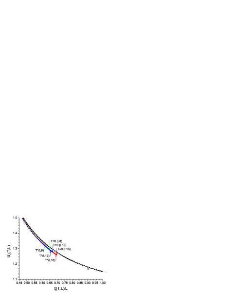
Figure 8: (Color on line) The Binder cumulant $U_{4}(\beta,L)$ as a function of the normalized second-moment correlation length $\xi(\beta,L)/L$ for the Gaussian model ($L=8$ black triangles, $L=12$ black circles, $L=16$ black squares) and for the bimodal model ($L=8$ green triangles, $L=12$ blue circles, $L=16$ red squares). Zero temperature end-points and crossover temperature $T^{*}(L)$ points as indicated. Open square : 2D Ising model critical point salas:00 .

VI Discussion

We can briefly review the articles which suggest that the bimodal $\eta$ is zero at $T>0$. Jörg et al. jorg:06 made the claim that ”The [2D ISG] $T>0$ properties fall into just one universality class” on the basis of their numerical scaling plot. It has already been pointed out in Ref. katzgraber:07 that the Ref. jorg:06 Fig. 2 points are derived using an extrapolation procedure which is not valid for the bimodal model. From a careful inspection of Ref. jorg:06 Fig. 2 it can be seen that the bimodal (blue) points do not actually lie on the indicated $\eta=0$ ”fit” line. Thus there is no firm basis from the Ref. jorg:06 data for the universality claim.

Parisen Toldin et al. parisen:10 ; parisen:11 also claim that ”The analysis …confirms that [the Gaussian and bimodal models] belong to the same universality class”. Fig. 1 of Ref. parisen:11 presents data for the Gaussian and bimodal models, (and for another discrete interaction distribution model) in the form of plots of the Binder cumulant $U_{4}(T,L)$ against the normalized correlation length $\xi(T,L)/L$ as in the present Fig. 8. It is stated “Thus, these [Fig. 1] results […] confirm that all models belong to the same universality class.” On the contrary, as discussed in the previous section, our analogous (but more precise) plots for Gaussian and bimodal data, Fig. 8, demonstrate that the two models are manifestly in different universality classes.

Fernandez et al. fernandez:16 also claim that from their analysis “Universality among binary and Gaussian couplings is confirmed to a high numerical accuracy.” They explicitly do not investigate the $T\sim 0$ region nor the crossover” but the same bimodal end-point behavior as in the present Fig. 8 or Ref. parisen:11 Fig. 1 can be inferred by inspection of the raw $\xi(L,T)/L$ data of Ref. fernandez:16 Fig. 1, leading again to the same conclusion as in the previous section. The final ”high numerical accuracy” bimodal exponent estimate $|\eta|<0.02$ of Ref. fernandez:16 (which is incompatible with their ”Quotient” data, reproduced in Ref. lundow:17 ) can be traced to an algebraic error in the derivation of their scaling rule expression C1 (see discussion in Ref. lundow:17 ).

VII Conclusion

The present measurements confirm remarkably well the main conclusion drawn from the pioneering 1983 work of McMillan mcmillan:83 , i.e., an effective exponent $\eta\sim 0.28$ for the bimodal 2D ISG at temperatures in what is now classified as being well in the $T>T^{*}(L)$ regime. Equivalent 2D Gaussian $G(R)$ data in the same temperature range can be fitted satisfactorily assuming an effective exponent equal to the known Gaussian critical value,$\eta\equiv 0$.

A careful comparison of of Binder cumulant $U_{4}(\beta,L)$ against normalized correlation length $\xi(\beta,L)/L$ Gaussian and bimodal data show bimodal end-point behavior incompatible with $\eta=0$ so confirming that the Gaussian and bimodal 2D ISG models are not in the same universality class note2 .

Universality in 2D ISGs in the $T>T^{*}(L)$ regime as claimed by Jörg et al. jorg:06 , by Parisen Toldin et al. parisen:10 , and by Fernandez et al. fernandez:16 is incompatible with measurements made by other groups over 35 years for $T$ both above and below $T^{*}(L)$: Refs. mcmillan:83 ; wang:88 ; houdayer:01 ; katzgraber:05 ; katzgraber:07 ; lundow:16 ; lundow:17 , and the present results.

Systems showing dependence of critical exponents on model parameters are few and far between. Even Baxter’s 8-vertex model baxter:71 shows ”weak universality”, with constant $\eta$, which is not the case for the 2D ISGs. A further important implication of the empirical demonstration of non-universality for ISGs in dimension two is that there seems no firm reason to suppose that standard universality rules hold for ISGs in higher dimensions either. Indeed we have presented strong evidence for breakdown of Universality in ISGs in dimensions four and five also lundow:15 ; lundow:15a ; lundow:17a .

It was stated fifteen years ago that ”classical tools of RGT analysis are not suitable for spin glasses” parisi:01 but this approach castellana:11 ; angelini:13 has not yet converged on predictions concerning non-universality.

References

- (1) S. F. Edwards and P. W. Anderson, J. Phys. F 5, 965 (1975).
- (2) M. Ohzeki and H. Nishimori, J. Phys. A: Math. Theor. 42, 332001 (2009).
- (3) A. K. Hartmann and A. P. Young, Phys. Rev. B 66, 094419 (2002).
- (4) A. C. Carter, A. J. Bray, and M. A. Moore, Phys. Rev. Lett. 88, 077201 (2002).
- (5) A. K. Hartmann, A. J. Bray, A. C. Carter, M. A. Moore, and A. P. Young, Phys. Rev. B 66, 224401 (2002).
- (6) J. Houdayer and A. K. Hartmann, Phys. Rev. B 70, 014418 (2004).
- (7) P. H. Lundow and I. A. Campbell, Phys. Rev. E 93, 022119 (2016).
- (8) L. A. Fernandez, E. Marinari, V. Martin-Mayor, G. Parisi, and J. J. Ruiz-Lorenzo, Phys. Rev. B 94, 024402 (2016).
- (9) P. H. Lundow and I. A. Campbell, Phys. Rev. E 95, 042107 (2017).
- (10) T. Jörg, J. Lukic, E. Marinari, O. C. Martin, Phys. Rev. Lett. 96, 237205 (2006).
- (11) C. K. Thomas, D. A. Huse, and A. A. Middleton, Phys. Rev. Lett. 107, 047203 (2011).
- (12) Y. Ozeki, J. Phys. Soc. Jpn. 59, 3531 (1990).
- (13) J. Poulter and J. A. Blackman, Phys. Rev. B 72, 104422 (2005).
- (14) A. K. Hartmann, Phys. Rev. B 77, 144418 (2008).
- (15) I. Morgenstern and K. Binder, Phys. Rev. B 22, 288 (1980).
- (16) W. L. McMillan, Phys. Rev. B 28, 5216 (1983).
- (17) K. Hukushima and K. Nemoto, J. Phys. Soc. Japan 65, 1604 (1996).
- (18) J. -S. Wang and R. H. Swendsen, Phys. Rev. B 38, 4840 (1988).
- (19) This sophisticated technique wang:88 appears to be very reliable; in the same publication it was validated by 2D Ising model measurements, and in addition to the bimodal 2D ISG estimate it also provided estimates for bimodal ISG values in 3D and in 4D which are close to recent estimation (thirty years later) from standard simulation measurements.
- (20) J. Houdayer, Eur. Phys. J. B 22, 479 (2001).
- (21) H. G. Katzgraber and Lik Wee Lee, Phys. Rev. B 71, 134404 (2005).
- (22) H. G. Katzgraber, Lik Wee Lee, and I. A. Campbell, Phys. Rev. B 75, 014412 (2007).
- (23) In the much simpler fully frustrated 2D Ising model the ThL “effectively continuous energy level” regime effective exponent and the exponent are both equal to lundow:17 . In 2D the bimodal ISG also the ”transition” does not seem to modify .
- (24) A. L. Talapov, V. B. Andreichenko, Vl. S. Dotsenko, L. N. Shchur, Int. J. Mod. Phys. C 4 787 (1993).
- (25) P. Butera and M. Comi, Phys. Rev. B 69 174416 (2004).
- (26) F. Parisen Toldin, A. Pelissetto, and E. Vicari, Phys. Rev. E 82, 021106 (2010).
- (27) F. Parisen Toldin, A. Pelissetto, and E. Vicari, Phys. Rev. E 84, 051116 (2011).
- (28) J. Salas and A. D. Sokal, J. Stat. Phys. 98, 551 (2000).
- (29) R. J. Baxter, Phys. Rev. Lett., 26, 832 (1971).
- (30) P. H. Lundow and I. A. Campbell, Phys. Rev. E 91, 042121 (2015).
- (31) P. H. Lundow and I. A. Campbell, Physica A 434 181 (2015).
- (32) P. H. Lundow and I. A. Campbell, Phys. Rev. E 95, 012112 (2017).
- (33) G. Parisi, R. Petronzio, F. Rosati, Eur. Phys. J. B 21 605 (2001).
- (34) M. Castellana, Europhys. Lett. 95 47014 (2011).
- (35) M. C. Angelini, G. Parisi, F. Ricci-Tersenghi, Phys. Rev. B 87 134201, (2013).
- (36) We find that all continuous distribution 2D ISG models constitute a single universality class but that each discrete distribution 2D ISG model belongs to an individual class lundow:17 ).