Fiber-Flux Diffusion Density for White Matter Tracts Analysis: Application to Mild Anomalies Localization in Contact Sports Players

Abstract

We present the concept of fiber-flux density for locally quantifying white matter (WM) fiber bundles. By combining scalar diffusivity measures (e.g., fractional anisotropy) with fiber-flux measurements, we define new local descriptors called Fiber-Flux Diffusion Density (FFDD) vectors. Applying each descriptor throughout fiber bundles allows along-tract coupling of a specific diffusion measure with geometrical properties, such as fiber orientation and coherence. A key step in the proposed framework is the construction of an FFDD dissimilarity measure for sub-voxel alignment of fiber bundles, based on the fast marching method (FMM). The obtained aligned WM tract-profiles enable meaningful inter-subject comparisons and group-wise statistical analysis. We demonstrate our method using two different datasets of contact sports players. Along-tract pairwise comparison as well as group-wise analysis, with respect to non-player healthy controls, reveal significant and spatially-consistent FFDD anomalies. Comparing our method with along-tract FA analysis shows improved sensitivity to subtle structural anomalies in football players over standard FA measurements.

1 Introduction

WM tractography from diffusion tensor imaging (DTI) is an efficient tool for longitudinal analysis and group studies, in particular when standard magnetic resonance imaging (MRI) is not sufficiently sensitive to detect subtle structural anomalies, such as in mild traumatic brain injury (mTBI) [24]. The fiber bundles rendered by tractography, in the form of streamline 3D coordinates, can be represented by geometrical properties as well as diffusivity measures (e.g., fractional anisotropy - FA, mean diffusivity - MD, axial diffusivity - AD, radial diffusivity - RD). Nevertheless, coherent mathematical modeling of the bundles, for along-tract pair-wise comparison and group-wise analysis, is a challenging task. The main difficulty is finding a common parameterization to faithfully represent the many fibers within a single bundle, and to match different bundles.

A straight-forward parameterization considers the natural grid of the images. Often, voxel-based registration of the MRI volumes is performed prior to the modeling. However, whole-brain registration does not guarantee an optimal alignment between corresponding fiber tracts due to large topological differences [12, 21, 28]. Therefore, most along-tract analysis approaches use arc-length (equidistant) re-parameterization prior to quantitative analysis [7, 16, 19, 26], and sometimes use anatomical landmarks [17] or crop the tract edges [28] to refine the alignment. Alternatively, tractography-based registration methods directly align sets of fibers based on their geometry and shape, using their streamline 3D coordinates, e.g., [12, 20].

A different paradigm considers parameterization that is intrinsic to specific bundles. Yushkevich et al. [31] used a parametric medial-surface representation of thin sheet-like fiber structures, by projecting the volumetric data into a 2-manifold. In a similar manner, tube-like shaped fiber bundles were modeled by their average (midline) trajectory in [5, 8, 11]. A more recent method suggests using manifold learning to achieve joint parameterization of fiber bundles, by mapping corresponding tracts across subjects into a latent bundle core [15]. Other approaches circumvent the parameterization problem altogether. In [9], a metric on WM fiber bundles is defined by the path integral of the fibers modeled as currents with an optimally constructed vector field. This approach has been extended in [4], using varifolds. However, [4, 9] do not provide along-tract analysis.

The contribution of the proposed framework is two-fold, referring to both fiber bundle modeling and alignment. Aiming to perform quantitative along-tract analysis, we introduce the concept of Fiber-Flux Diffusion Density (FFDD) descriptors that couple the bundle’s geometry with local diffusivity measures. This allows diffusion-related features to be accounted for, as well as structural variations along tracts, which may not be reflected by diffusion scalars alone. Fiber bundle modeling, in the form of tract-profiles, is obtained by application of these descriptors along the mean trajectory of the bundle. Fiber tracts alignment is addressed as a curve matching problem between the mean trajectories of the tracts. The proposed dissimilarity measure is based on FFDD tract profiles, thus utilizing both diffusional and geometrical information for the alignment task, rather than relying exclusively on geometrical properties (e.g., arc-length and curvature) as in classical curve matching algorithms [22, 30], or on scalar measurements as in FA-based registration methods [1, 25]. Moreover, unlike traditional curve matching approaches [6, 30], we do not map one curve into another. Instead, we adapt the FMM for curve alignment [10], to symmetrically match pairs of tracts with sub-voxel accuracy, based on FFDD dissimilarities as an inverse speed map. The proposed alignment framework plays a key role in the construction of standardized FFDD profiles that can be considered as a bundle-specific atlas. This atlas facilitates group-wise statistical analysis for the assessment and localization of abnormalities in WM fiber tracts.

We demonstrate the validity of our method by performing a tract-specific longitudinal analysis of a basketball player diagnosed with occipital mTBI and a frontal hemorrhage, having scans one week and 6 months post-injury. We further conduct a cross-sectional study, comparing 13 professional American-football players with possible mTBIs, with 17 normal control (NC) subjects. The analysis includes five major white matter tracts: the left and right fronto-occipital fasciculus (IFOF), left and right corticospinal tract (CST), and the forceps minor tract (FMT). Substantial FFDD abnormalities were found in several football players compared to controls, mostly located at the occipital part of the IFOF and at the central part of the forceps minor. The same regions also demonstrate statistically significant FFDD differences between the groups, indicated by low p-values and high standard deviation (STD). For some players, repeated scans revealed consistent and increased FFDD anomalies with time, even after a few weeks off-season. Results are in line with mTBI findings from DTI [14]. We also demonstrate that the proposed FFDD method provides improved sensitivity to subtle structural anomalies compared to along-tract FA analysis, due to the use of additional geometric information.

The rest of the paper is organized as follows: Section 2 presents the FFDD descriptors, followed by an introduction of the proposed framework for fiber bundles alignment and statistical analysis. Section 3 presents experimental results for two different datasets of contact-sport players. We conclude in section 4.

2 Methods

2.1 Fiber-Flux Diffusion Density Descriptor

A fiber bundle $\displaystyle\mathcal{B}$ can be thought of as a set of similar trajectories with a common origin and destination, along which water molecules are diffused [13]. In the spirit of this notion, we define a local measure for quantifying the fiber-flux of $\displaystyle\mathcal{B}$ through a given plane $\displaystyle\pi$, with normal $\displaystyle\hat{n}_{\pi}\left(p\right)$ at point $\displaystyle p\in\pi$, i.e.,

$$\mathcal{F_{B}\mathit{\left(\pi;p\right)}=}\frac{1}{N_{p}}\stackrel{{\scriptstyle[}}{{i}}=1]{N_{p}}{\sum}\hat{\tau}_{i}\left(x_{i}\right)\cdot\hat{n}_{\pi}\left(p\right),$$ (1)

where $\displaystyle N_{p}$ is the number of intersected fibers, $\displaystyle\xi=\left\{x_{i}\right\}$ is the set of intersection points between the plane and the fiber bundle, and $\displaystyle\left\{\hat{\tau}_{i}\left(x_{i}\right)\right\}$ are the tangents of the fibers at those points. We call $\displaystyle\mathcal{F_{B}}\mathit{\left(\pi;p\right)}$ the fiber-flux density (FFD) of bundle $\displaystyle\mathcal{B}$ at point $\displaystyle p$. The plane $\displaystyle\pi$ is oriented such that the fiber-flux is maximized, i.e., $\displaystyle\hat{n}_{\pi}\left(p\right)=\arg\underset{\hat{n}_{\pi}}{\max}\,\mathcal{F_{B}}\mathit{\left(\pi;p\right)}$. We use an iterative approach to solve this maximization problem in the spirit of [27]. We further introduce diffusivity properties into our model by extending the FFD measure. Let $\displaystyle\mathcal{S}\left(x_{i}\right)$ define a diffusivity scalar of choice (FA, MD, AD, or RD), associated with the point $\displaystyle x_{i}$. We define the fiber-flux diffusion density (FFDD) as follows:

$$\mathcal{J_{B}\mathit{\left(\pi;p\right)}=}\frac{1}{N_{p}}\stackrel{{\scriptstyle[}}{{i}}=1]{N_{p}}{\sum}\mathcal{S}\left(x_{i}\right)\hat{\tau}_{i}\left(x_{i}\right)\cdot\hat{n}_{\pi}\left(p\right)$$ (2)

In practice, we refer to the FFDD as a vector $\displaystyle\mathcal{\vec{J}}_{\mathcal{B}}\mathit{\left(p\right)}=\mathcal{\mathcal{J}_{B}}\mathit{\left(p\right)}\hat{n}\left(p\right)$ to account for the local orientation of the fiber bundle. Note that the set of four FFDD descriptors (each assigned with a different diffusivity measure) couples diffusion measures with local geometrical features of the bundle. For example, local differences in orientation are taken into account, and regions with “incoherent” fiber orientations are “punished” by having lower FFDD values.

2.2 Along Tract Profiles

We calculate the mean fiber of the bundle $\displaystyle c(s)=\left(x\left(s\right),y\left(s\right),z\left(s\right)\right)$, where $\displaystyle s$ is its arc-length parameter, based on Fourier descriptor [5]. According to this method, individual streamline fibers are represented by the coefficients of cosine series expansions, which are computed from tractography data using least squares estimation. The mean fiber is then optimally obtained by averaging the representation coefficients and applying the inverse transformation. The locations of the planar cross-sections along the bundle are determined by equidistant sampling points along the mean fiber $\displaystyle\left\{p_{m}\right\}=\left\{c(s^{m})\right\}_{m=1}^{M}$. Tract-profiles $\displaystyle\left\{\mathit{\mathcal{\vec{J}}_{\mathcal{B}}\mathit{\left(p_{m}\right)}}\right\}_{m}$ are obtained by applying the FFDD descriptors along the tract, over these points.

2.3 Fiber Bundles Alignment

We address the alignment of two bundles $\displaystyle\mathcal{B}_{1}$ and $\displaystyle\mathcal{B}_{2}$ as a curve-matching problem between their mean fibers $\displaystyle c_{1}\left(s_{1}\right)$ and $\displaystyle c_{2}\left(s_{2}\right)$, where $\displaystyle s_{1}\in\left[0\,,\,L_{1}\right]$ and $\displaystyle s_{2}\in\left[0\,,\,L_{2}\right]$ are the respective arc-length parameterizations. We adapt the FMM-based symmetrical curve matching framework of [10] to allow sub-sampling resolution of the alignment. Nevertheless, rather than using geometrical properties alone for the construction of the inverse speed map $\displaystyle F\left(s_{1},s_{2}\right)$, we propose a new dissimilarity measure which relies on the FFDD profiles:

$$F\left(s_{1},s_{2}\right)=\left\|\mathcal{\vec{J}}_{\mathcal{B_{\mathrm{1}}}}\mathit{\left(s_{1}\right)}-\mathcal{\vec{J}}_{\mathcal{B_{\mathrm{2}}}}\mathit{\left(s_{2}\right)}\right\|+\lambda$$ (3)

where $\displaystyle\lambda$ is a scalar used for regularization, set as in [10]. Given $\displaystyle F\left(s_{1},s_{2}\right)$, the FMM solves the Eikonal equation $\displaystyle\left|\nabla T\left(s_{1},s_{2}\right)\right|=F\left(s_{1},s_{2}\right)\,\,\forall\,s_{1},s_{1},$ providing as output the weighted distance matrix $\displaystyle T\left(s_{1},s_{2}\right).$ Fig.1a-b present $\displaystyle F\left(s_{1},s_{2}\right)$ and $\displaystyle T\left(s_{1},s_{2}\right)$, respectively. The optimal alignment is then defined by the shortest path in $\displaystyle F\left(s_{1},s_{2}\right)$ from the starting point $\displaystyle\left(0,0\right)$ to the endpoint $\displaystyle\left(L_{1},L_{2}\right)$. The alignment path $\displaystyle\alpha\left(\tau\right)=\left(s_{1}\left(\tau\right),s_{2}\left(\tau\right)\right)$ defines pairs of matching points between the bundles, and is computed with sub-voxel resolution as follows:

$$\alpha\left(\tau-\varepsilon\right)=\alpha\left(\tau\right)-\varepsilon\nabla T\left(s_{1},s_{2}\right)\,\,;\,\,\alpha\left(\mathcal{L}\right)=\left(L_{1},L_{2}\right)$$ (4)

as illustrated in Fig. 1c. The step size $\displaystyle\varepsilon$ is usually set to some small value ($\displaystyle\varepsilon\ll 1).$ For uniformity, we re-sample $\displaystyle\alpha$ into $\displaystyle M$ samples, i.e., $\displaystyle\left\{\alpha\left(\tau^{m}\right)\right\}_{m=1}^{M}$, such that the aligned mean fibers are obtained by $\displaystyle\tilde{C}_{1}=\left\{c_{1}\left(s_{1}\left(\tau^{m}\right)\right)\right\}_{m=1}^{M}$ and $\displaystyle\tilde{C}_{2}=\left\{c_{2}\left(s_{2}\left(\tau^{m}\right)\right)\right\}_{m=1}^{M}$ (see Fig. 1d), and their tract-profiles are aligned accordingly: $\displaystyle\tilde{J_{\mathcal{B}_{1}}}=\left\{\mathcal{\vec{J}}_{\mathcal{B_{\mathrm{1}}}}\mathit{\left(c_{1}\left(s_{1}\left(\tau^{m}\right)\right)\right)}\right\}_{m=1}^{M}$ and $\displaystyle\tilde{J_{\mathcal{B}_{2}}}=\left\{\mathcal{\vec{J}}_{\mathcal{B_{\mathrm{2}}}}\mathit{\left(c_{2}\left(s_{2}\left(\tau^{m}\right)\right)\right)}\right\}_{m=1}^{M}$.

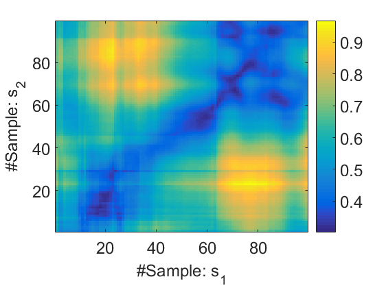
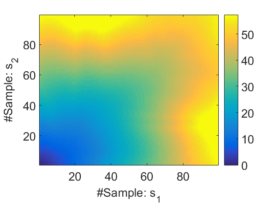
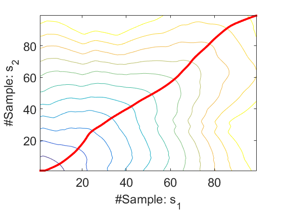
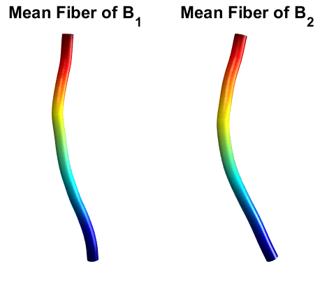
(a) $\displaystyle F\left(s_{1},s_{2}\right)$	(b) $\displaystyle T\left(s_{1},s_{2}\right)$	(c) Compute $\displaystyle\alpha$	(d) Aligned Curves

Figure 1: Alignment using FMM. (a) Local dissimilarities $\displaystyle F\left(s_{1},s_{2}\right)$ based on FFDD profiles. (b) $\displaystyle T\left(s_{1},s_{2}\right)$ is obtained by solving the Eikonal equation. (c) The alignment path $\displaystyle\alpha\left(\tau\right)$ is computed by backtracking along the gradients of $\displaystyle T\left(s_{1},s_{2}\right)$. (d) Resulting alignment (color-coded).

2.4 Along-Tract Variability Analysis

Pairwise Comparison: Let $\displaystyle\tilde{J_{\mathcal{B}_{1}}}$ and $\displaystyle\tilde{J_{\mathcal{B}_{2}}}$ be a pair of aligned tract-profiles to be compared, e.g., of a subject-specific tract in two longitudinal scans. We define a pointwise dissimilarity measure between them as follows:

$$d_{\mathcal{J}}\left(\mathcal{B}_{1},\mathcal{B}_{2};\alpha\left(\tau^{m}\right)\right)=\left\|\mathcal{\vec{J}}_{\mathcal{B_{\mathrm{1}}}}\mathit{\left(c_{1}\left(s_{1}\left(\tau^{m}\right)\right)\right)}-\mathcal{\vec{J}}_{\mathcal{B_{\mathrm{2}}}}\mathit{\left(c_{2}\left(s_{2}\left(\tau^{m}\right)\right)\right)}\right\|$$ (5)

Although we focus here on computing local dissimilarities along the two bundles, global dissimilarity can also be calculated: $\displaystyle D_{\mathcal{J}}\left(\mathcal{B}_{1},\mathcal{B}_{2}\right)=\underset{\alpha}{\int}d_{\mathcal{J}}\left(\mathcal{B}_{1},\mathcal{B}_{2};\alpha\left(\tau\right)\right)d\alpha$.

Group-Wise Statistical Analysis: Alignment of multiple fiber tracts for group-wise analysis is performed as follows. Let $\displaystyle\mathcal{J_{\mathrm{\mathit{g}}}=}\left\{\mathcal{\vec{J}}_{\mathcal{B_{\mathrm{n}}}}\left(s\right)\right\}_{n=1}^{\mathcal{N}_{g}}$ denote the set of $\displaystyle\mathcal{N}_{g}$ tract-profiles of a group of subjects, and let $\displaystyle\mathcal{C_{\mathit{g}}=}\left\{C_{n}\left(s\right)\right\}_{n=1}^{\mathcal{N}_{g}}$ denote their respective mean fibers with a joint arc-length parameterization $\displaystyle s$. We define a reference tract profile, with its corresponding mean fiber as follows:

$$\mathcal{\vec{J}}_{ref}\left(s\right)=\frac{1}{\mathcal{N}_{g}}\stackrel{{\scriptstyle[}}{{n}}=1]{\mathcal{N}_{g}}{\sum}\mathcal{\vec{J}}_{\mathcal{B_{\mathrm{n}}}}\left(s\right)\,\,,\,\,C_{ref}\left(s\right)=\frac{1}{\mathcal{N}_{g}}\stackrel{{\scriptstyle[}}{{n}}=1]{\mathcal{N}_{g}}{\sum}C_{n}\left(s\right)$$ (6)

Alignment of the tract-profiles is obtained by first mapping each of them to the reference tract as discussed in Section 2.3. We then interpolate the resulting alignment paths $\displaystyle\left\{\alpha\left(\tau_{n}\right)\right\}_{n=1}^{\mathcal{N}_{g}}$ such that they all contain the same set of $\displaystyle M$ samples of the reference tract $\displaystyle\left\{C_{ref}\left(s^{m}\right)\right\}_{m=1}^{M}$. We construct a bundle-specific atlas by pointwise averaging the aligned tract-profiles. This atlas represents the standardized tract-profile of the group, which is used as a benchmark for group-wise statistical analysis.

3 Experimental Results

We demonstrate our FFDD method on two different datasets of contact-sports players. Normal control (NC) group includes scans of healthy age-matched males. Diffusion weighted images (DWI) of all subjects were acquired on a 3T Philips Ingenia scanner using a single-shot, spin-echo, echo-planar imaging (EPI) sequence (TE=106 ms, TR=9000 ms, FOV = 224x224x120 mm). A total of 60 2[mm]-thick slices were acquired with 33 different gradient directions (b=1000 s/mm²) with a voxel resolution of 1.75$\displaystyle\times$1.75$\displaystyle\times$2 mm. Pre-Processing included rigid alignment to the SPM MNI T1-template; motion and eddy currents correction; DTI tensor model fitting [2]; and Tractography of five major tracts: left and right IFOF, left and right CST, and the FMT [29]. All performed by DSI Studio software (http://dsi-studio.labsolver.org/). The tracts were delineated by placing multiple regions of interest (ROIs) from the JHU WM atlas [18].

3.1 Longitudinal Case Study

We performed pairwise comparison between two scans of a 32-year-old basketball player, diagnosed with mild occipital traumatic brain injury and frontal hemorrhage due to contrecoup impact, acquired one week and 6 months post-injury. The hemorrhagic lesion at the frontal right hemisphere of the player is no longer visible in the FLAIR image acquired 6 months after injury (Fig. 2a). Local differences between corresponding, longitudinal FA- and MD-FFDD profiles of the FMT (chosen due to its proximity to the lesion area) are shown in Fig. 2d. Figs. 2b-c present color-coded FMT to visually demonstrate these differences. Results show significant longitudinal variability at the right hemisphere part of the tract, corresponding to the lesion area, and relatively minor differences along the rest of the tract. These results should be considered as a proof of concept, validating the FFDD analysis results for the detection and localization of mTBI-related variabilities between fiber bundles.

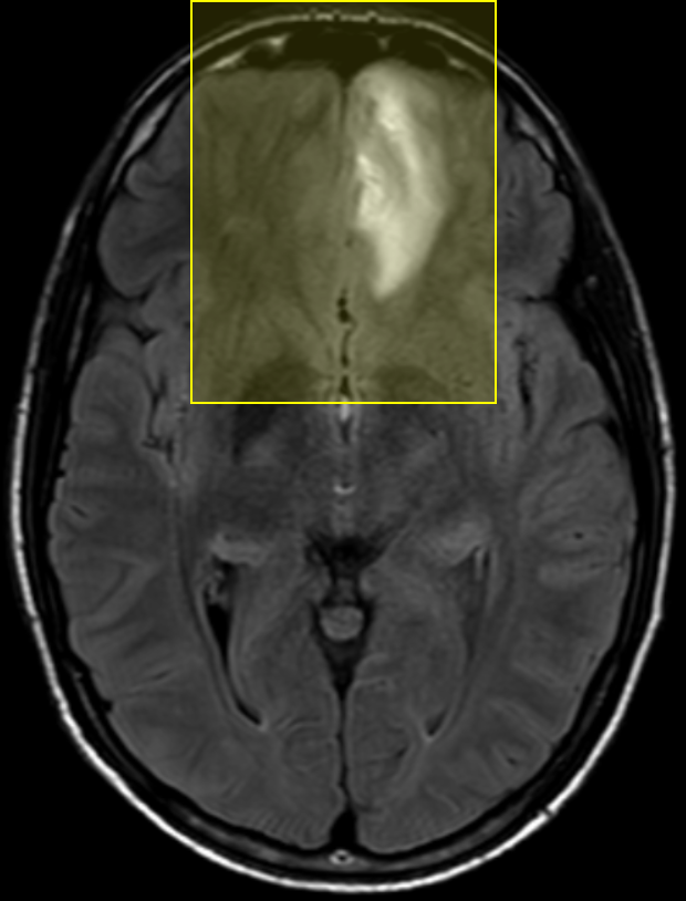
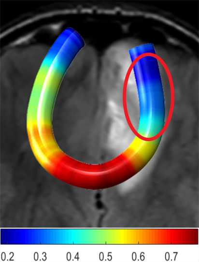
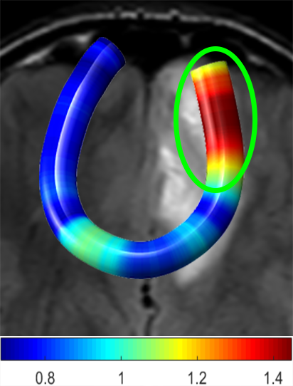
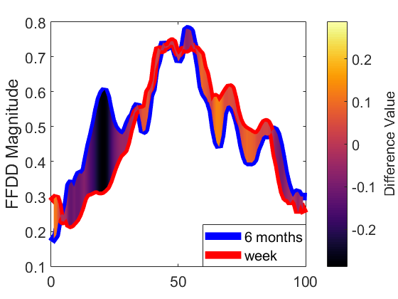
ONE WEEK					FA-FFDD
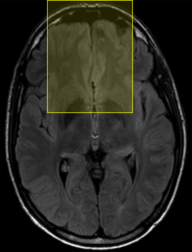
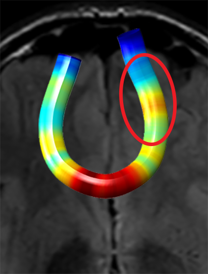
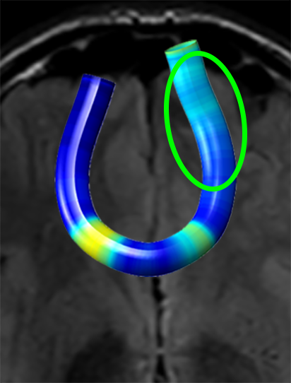
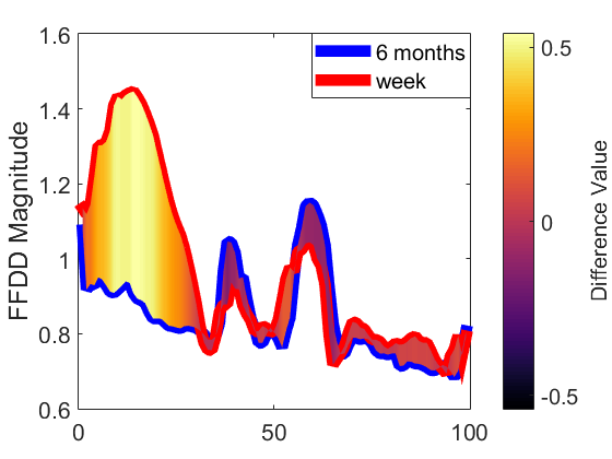
6 MONTHS					MD-FFDD
	(a) FLAIR	(b) FA-FFDD	(c) MD-FFDD	(d) Local Differences

Figure 2: Longitudinal FFDD analysis of the FMT. Right Panel: FA- and MD-based tract-profiles of both scans. Local differences are color-coded on the graph. Left Panel: FLAIR scans (axial slices), one week post-injury (top) and 6 months post-injury (bottom). (a) Highlighted boxes around the hemorrhaging area - lesion is no longer visible 6 months after injury. In (b) and (c) the tracts are colored-coded by the magnitude of their FFDD profiles. Regions with high longitudinal variability (marked in red and green ellipses) correspond to the lesion area.

3.2 Football Players Study

We analyzed 13 active professional American-football players (mean age = 28.3, STD = 6.4), with respect to 17 NCs (mean age = 26.1, STD = 2.3). For each subject, four FFDD tract-profiles were computed (based on FA, MD, RD, and AD), for each of the five examined tracts. The standardized FFDD profiles of NCs are shown in Fig. 3. Note that although FFDD values vary along the tracts, their profiles are consistent across subjects.

	Left IFOF	Right IFOF	Left CST	Right CST	Forceps Minor
Tract
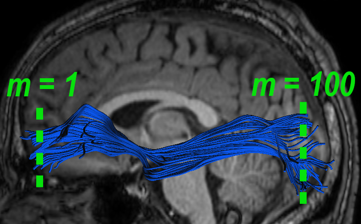
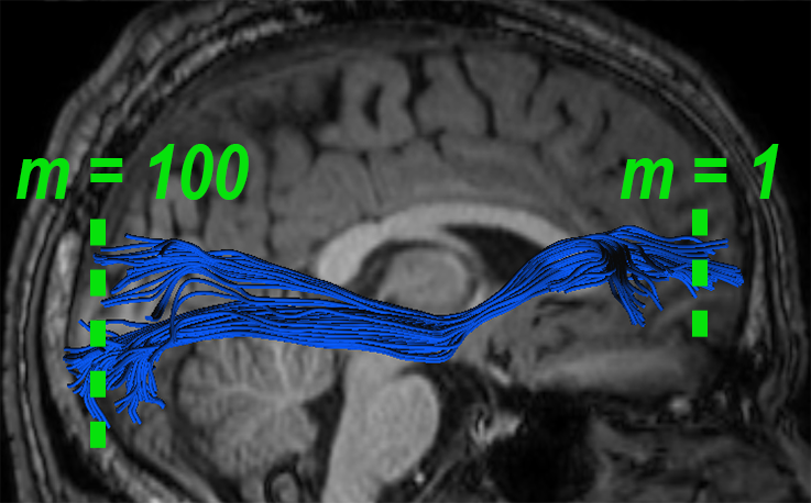
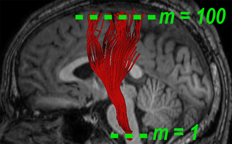
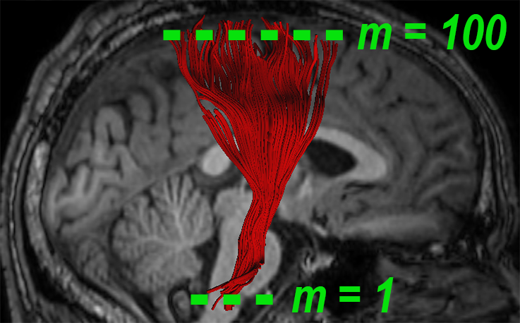
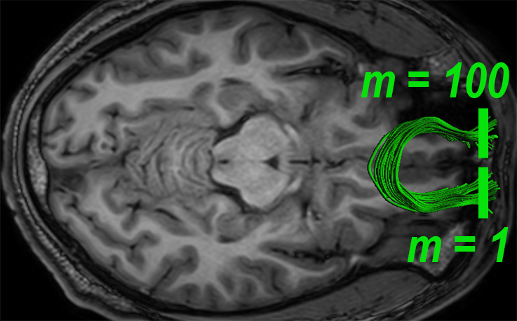
FA-FFDD
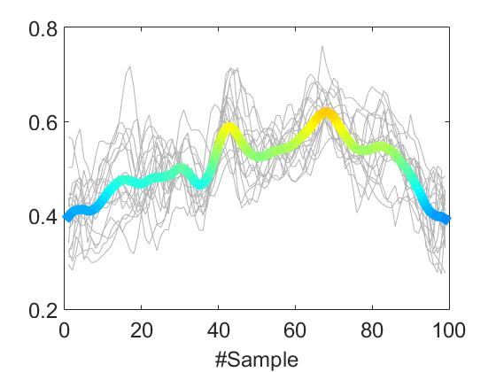
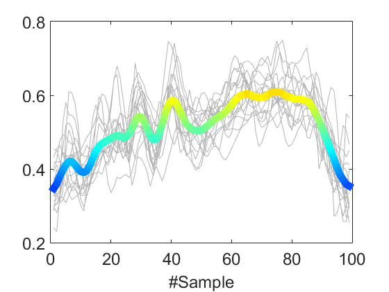
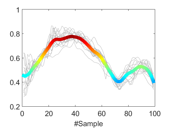
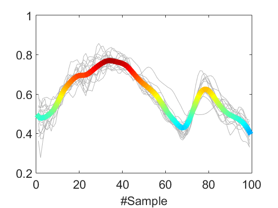
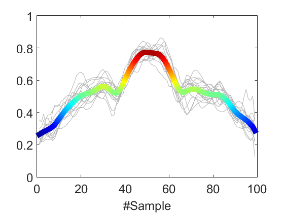
MD-FFDD
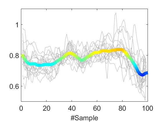
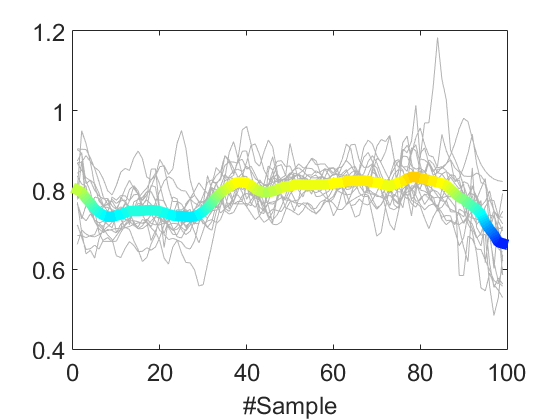
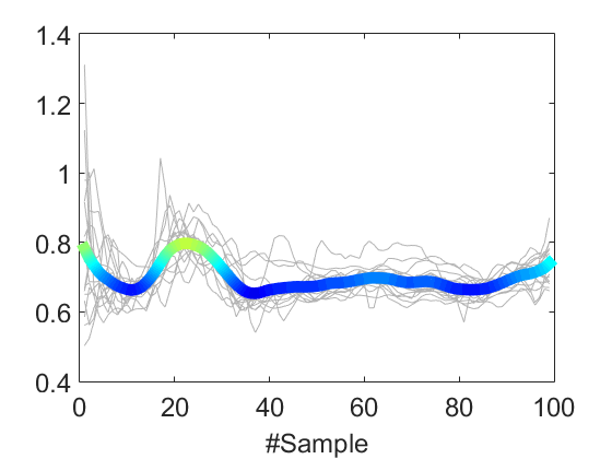
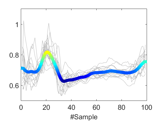
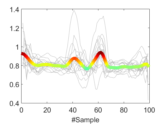
AD-FFDD
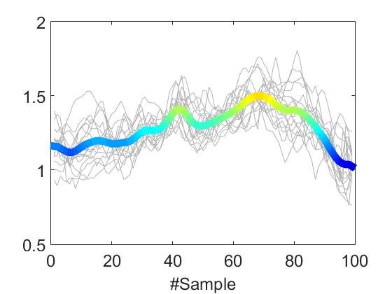
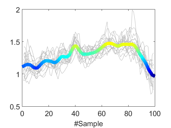
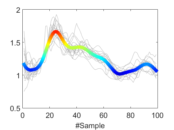
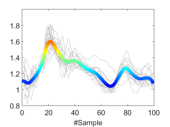
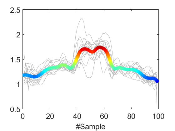
RD-FFDD

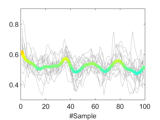
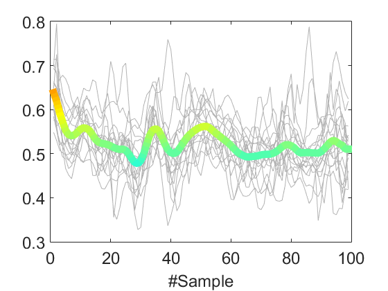
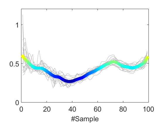
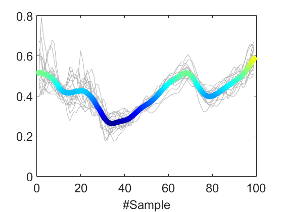
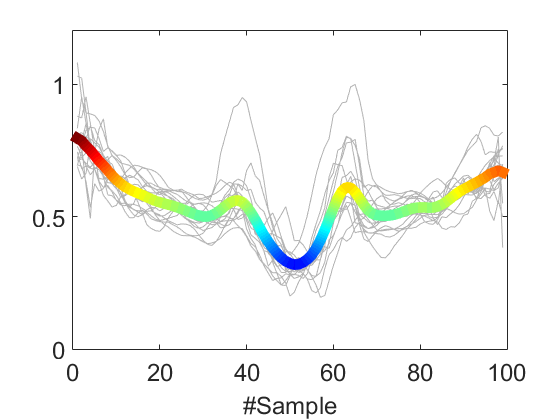
Figure 3: Top row: The 5 examined tracts. Bottom rows: Four types of standardized tract-profiles (colored): FA-FFDD, MD-FFDD, AD-FFDD, and RD-FFDD constructed from the aligned tract-profiles of NCs (gray).

Fig. 4 presents pointwise group-average and STD of MD-FFDD profiles of football players, demonstrating increased values at the occipital part of the left IFOF, and at the central part of the FMT, compared to NCs. Note that the football group also exhibits higher STD values compared to NCs, at the same areas along the tracts with increased group-average values. This statistical spread indicates that only a subset of the football players group has abnormal FFDD values, as expected.

	Pointwise Mean	$\displaystyle\mathrm{\Delta}$Mean	Pointwise STD	$\displaystyle\mathrm{\Delta}$STD
FMT
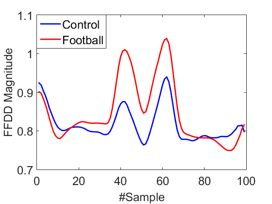
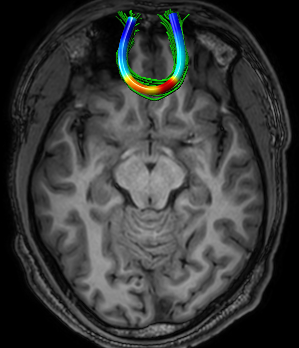
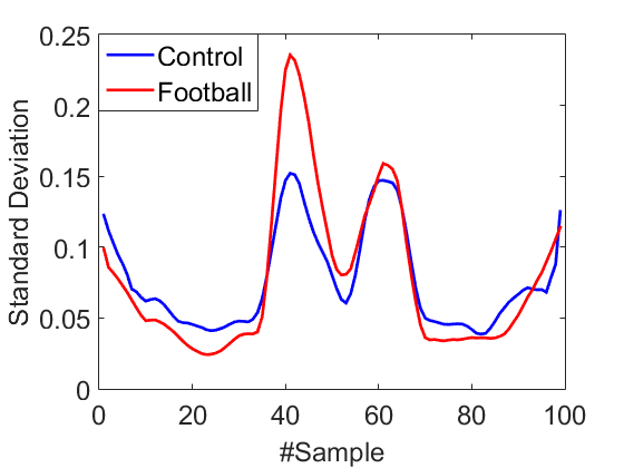
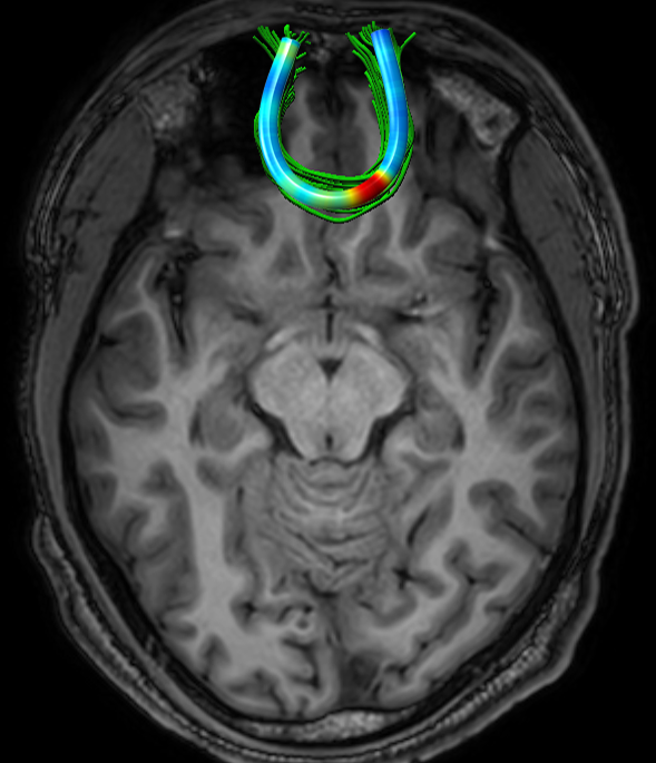
Left IFOF

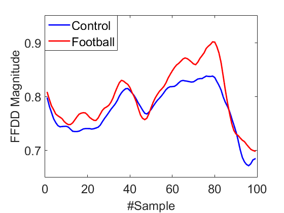
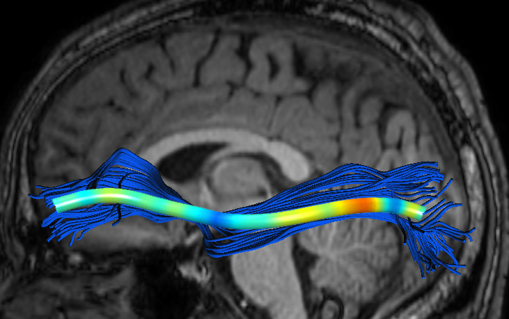
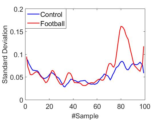
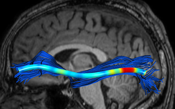
Figure 4: Group-wise statistical analysis based on MD-FFDD. Pointwise comparison of within-group average profile (left) and STDs (right) are presented for the FMT (top) and the left IFOF (bottom).

Our method also demonstrates statistically significant differences between the football and control groups (p-values < 0.05) at these regions of the IFOF and FMT, as shown in Fig. 5. The left panel of the figure presents an along-tract p-values analysis of the two tracts, calculated pointwise based on four different FFDD tract profiles and corrected for multiple comparisons using false detection rate (FDR) [3]. As reference, the right panel of the figure presents a p-values analysis based on whole tract average of conventional diffusivity measures extracted via DSI Studio, calculated using an unpaired T-test, which also shows statistically significant differences between the groups in the IFOF and FMT for some diffusion measures. These findings are further supported by a group-wise statistical analysis (mean and STD) of whole-tract average diffusivity measures (MD, AD, and RD), presented in Fig. 6. Results are in line with the FFDD analysis, demonstrating increased group-average diffusivity in the left IFOF and FMT of the football group compared to NCs. The figure also indicates the maximal value measured within the football group for each diffusivity measure. Note that for the left IFOF, player #11 demonstrates maximal values across all diffusivity measures, while the same applies to the FMT of player #12. We note that the CST did not present significant differences between the groups, in both FFDD and conventional analysis.

Left IFOF	Forceps Minor	Tracts-Average Analysis

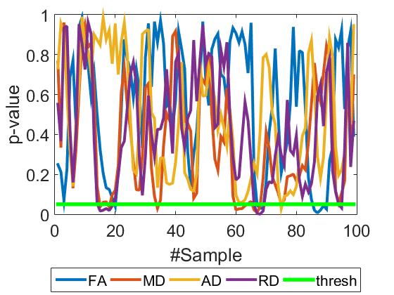
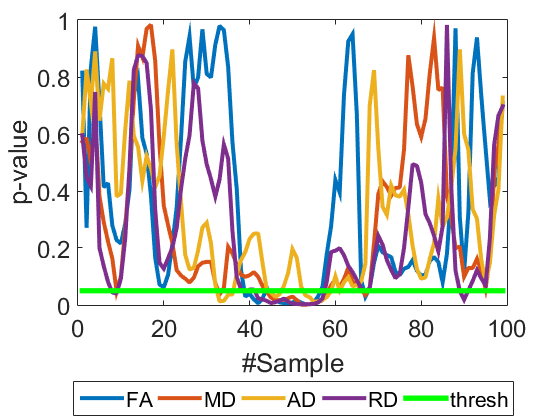
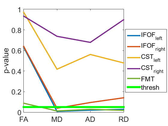
Figure 5: Group-wise p-values analysis. Left and middle: pointwise (corrected) p-values along the left IFOF and FMT, based on FFDD profiles. Most statistically significant differences between the groups (p-value<0.05) are located in the occipital part of the IFOF (samples #60 to #90) and central part of the FMT (samples #40 to #60). Right: scalar p-values based on tract-average diffusion measures (FA, MD, AD, and RD) of five different tracts. Statistically significant differences between the groups are shown for the left IFOF and FMT, in MD, AD, and RD measures.

	MD Analysis	AD Analysis	RD Analysis
Left IFOF
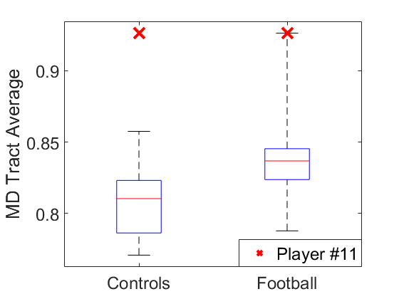
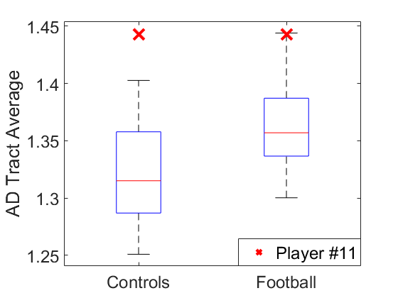
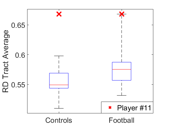
Forceps Minor

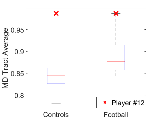
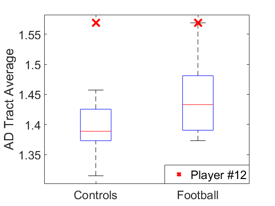
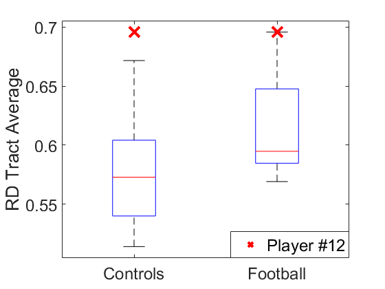
Figure 6: Box-plot group-wise statistical analysis of average diffusivity measures in the left IFOF (top) and FMT (bottom). Each box represents the distribution of values within the group: the red line represents the group-average value, the edges of the box represent the 25th and 75th precentiles of the group, and the edges of the dashed line represent the maximal and minimal values. The x symbol represents the maximal value measured in the football group. Note that for both tracts, the football group consistently demonstrates higher values across all diffusivity measures.

Experiments also showed significant FFDD longitudinal changes between mid-season and post-season scans in some football players. Fig. 7 presents mid- and post-season MD-FFDD profiles comparison of the left IFOF of one of the players, showing increased irregularities over time at the occipital part of the tract. Fig. 8 presents a similar MD-FFDD longitudinal analysis of the FMT of a different player, showing increased irregularities at the central part of the tract.

Mid vs. Post	Mid-season	Post-season
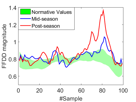
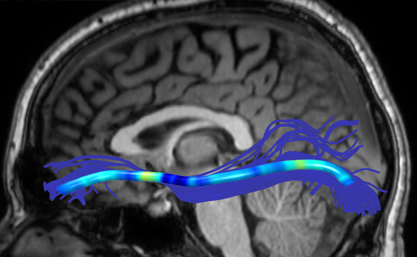
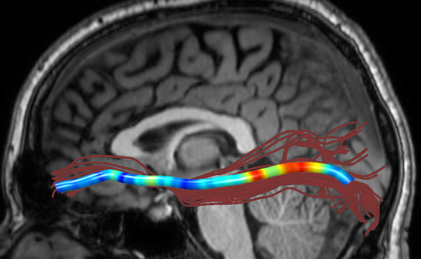
				STDs

Figure 7: MD-FFDD longitudinal changes in the left IFOF of player #11. Left: Mid-season and post-season tract-profiles in comparison to normative values ($\displaystyle\pm 1$ STD from standardized profile of NC). Middle and Right: Mid- and post-season abnormalities are color-coded along the tract (in units of #STDs from standardized profile). In the occipital area, mid-season profile demonstrates moderate abnormality (up to 2.5 STDs) while in post-season substantial abnormality (up to 6.5 STDs) is shown.

Mid vs. Post	Mid-season	Post-season
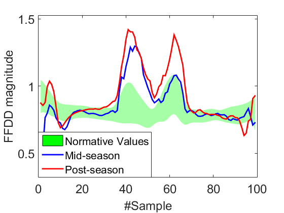
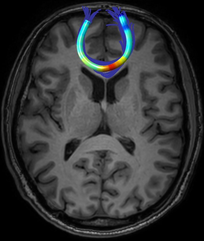
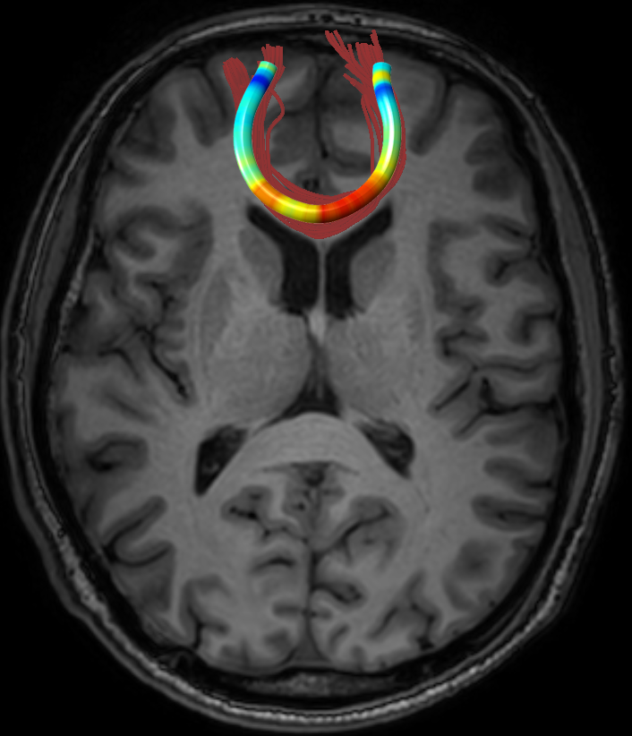
				STDs

Figure 8: MD-FFDD longitudinal changes along the FMT of player #12. Left: Mid-season and post-season tract-profiles are compared to normative values ($\displaystyle\pm 1$ STD from standardized profile of NCs). Middle and Right: Mid- and post-season abnormalities are color-coded along the tract (in units of #STDs from standardized profile). While mid-season profile demonstrates abnormality (up to 3.5 STDs) in a small region around the center of the tract, the post-season profile shows expansion in both magnitude (up to 4.5 STDs) and location of abnormality along the tract.

3.3 Sensitivity Analysis

In order to demonstrate the improved sensitivity of the proposed method in anomalies detection, we compared our FFDD groupwise analysis to an existing approach of along-tract analysis based on standard FA measurements. Similar to the FFDD analysis, normative values of standard FA were obtained by computing the pointwise mean and STD along the aligned FA profiles of NCs. The average FA profile of the football players group is then compared to these normative values. Fig. 9 presents a comparison between standard FA analysis and FA-FFDD analysis for the left and right IFOF. The comparison shows that while both methods yield similar results at the frontal and central parts of the tracts, the FA-FFDD analysis shows higher variation from NCs (1 STD) compared to standard FA (0.5 STD) at the occipital part of the tracts. Note that this finding is demonstrated symmetrically for the left and right IFOF, at a spatially-consistent location with the cross-sectional and longitudinal results presented earlier in this section. The improved sensitivity of FA-FFDD in this region over standard FA is due to the additional geometric information provided by the proposed descriptor, as demonstrated in Fig. 10, which shows the group-average fiber-flux density (FFD, no coupling with diffusion measurements) of football players and NCs along the left and right IFOF. Note that higher FFD variability between the groups is indeed located at the occipital part of the tracts.

	Left IFOF		Right IFOF
	(a) Football vs. NCs	(b) Variability from NCs	(a) Football vs. NCs	(b) Variability from NCs
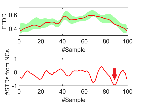
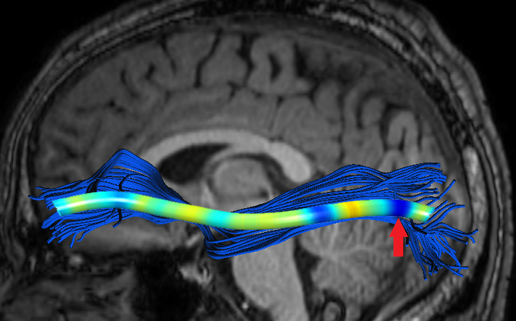
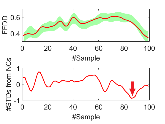
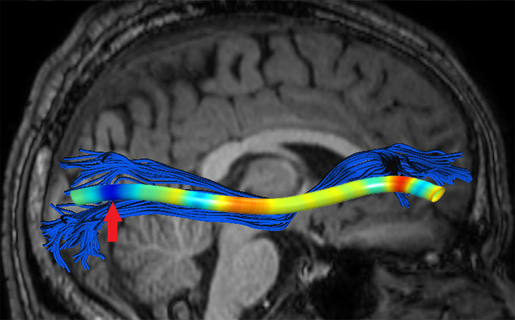
FA-FFDD						STDs
Standard FA

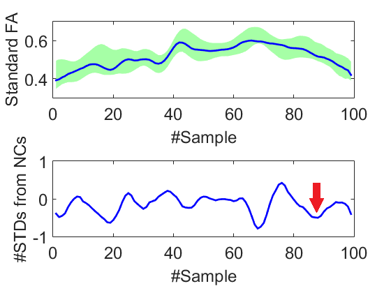
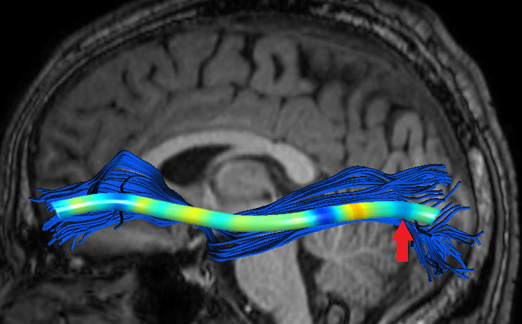
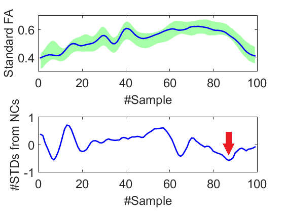
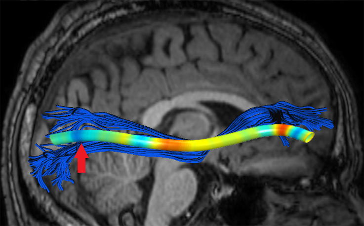
Figure 9: Comparison between groupwise statistical analysis based on FA-FFDD (top row) and standard FA (bottom row) for the left and right IFOF. (a) Pointwise average profile of post-season football group compared to normative values ($\displaystyle\pm 1$ STD from standardized profile of NCs). The red arrow points to the area in which FA-FFDD presents improved sensitivity in comparison to standard FA. (b) Deviation from NCs is color-coded along the tract (in units of #STDs from standardized profile).

Left IFOF			Right IFOF
(a) Football vs. NCs	(b) Pointwise differences		(a) Football vs. NCs	(b) Pointwise differences

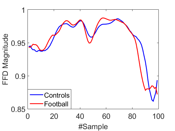
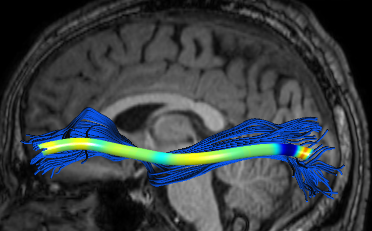
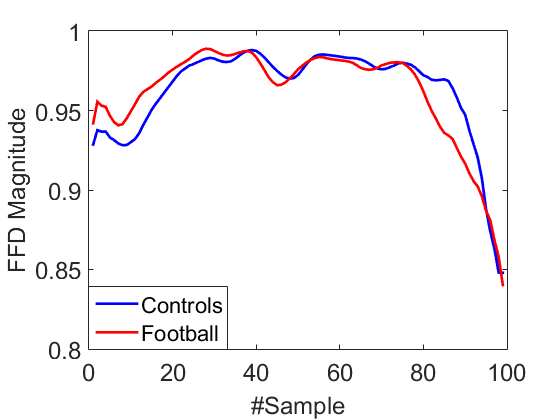
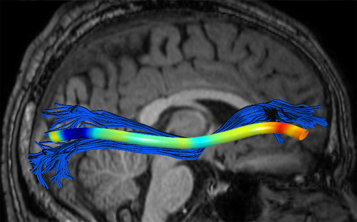
Figure 10: Groupwise statistical analysis based on geometric fiber-flux density (FFD) alone, with no diffusion measurements, for the left and right IFOF. (a) Pointwise comparison of within-group average FFD profiles between post-season football players and NCs. (b) Pointwise differences between the two profiles are color-coded along the tracts. The comparison shows increased flux-density variability between the groups at the occipital part of the tracts, allowing for increased sensitivity of the FFDD analysis in this area.

4 Summary and Conclusion

We presented a novel concept of FFDD descriptors that combine geometrical and diffusivity properties of WM fiber bundles, for local quantification of pairwise and group-wise differences. A sub-voxel alignment of tract profiles is accomplished by considering local FFDD dissimilarities as an FMM inverse speed map. This allows the construction of bundle-specific atlases for statistical analysis. Our method is demonstrated on two datasets of contact-sports players, revealing local WM tract anomalies. In a group-wise comparison between active football players and normal (non-players) controls, our method revealed statistically significant differences between the groups, at spatially-consistent areas within the IFOF and FMT tracts. Furthermore, our method presented improved sensitivity to subtle structural anomalies in football players compared to along-tract FA analysis. The obtained results suggest the proposed method as a promising tool for mTBI assessment and localization.

Acknowledgment

This research is partially supported by the Israel Science Foundation (T.R.R. 1638/16) and the IDF Medical Corps (T.R.R.).

References

- [1] Andersson, Jenkinson, Smith, et al. Non-linear registration, aka spatial normalisation fmrib technical report tr07ja2. FMRIB Analysis Group of the University of Oxford, 2, 2007.
- [2] P. Basser, J. Mattiello, and D. LeBihan. Estimation of the effective self-diffusion tensor from the NMR spin echo. JMR, pages 247–254, 1994.
- [3] Y. Benjamini and Y. Hochberg. Controlling the false discovery rate: a practical and powerful approach to multiple testing. Journal of the royal statistical society. Series B (Methodological), pages 289–300, 1995.
- [4] N. Charon and A. Trouvé. The varifold representation of nonoriented shapes for diffeomorphic registration. SIIMS, pages 2547–2580, 2013.
- [5] Chung, Adluru, Lee, et al. Cosine series representation of 3D curves and its application to white matter fiber bundles in diffusion tensor imaging. Statistics and its interface, page 69, 2010.
- [6] I. Cohen, N. Ayache, and P. Sulger. Tracking points on deformable objects using curvature information. In ECCV, pages 458–466, 1992.
- [7] Colby, Soderberg, Lebel, et al. Along-tract statistics allow for enhanced tractography analysis. Neuroimage, pages 3227–3242, 2012.
- [8] I. Corouge, S. Gouttard, and G. Gerig. Towards a shape model of white matter fiber bundles using diffusion tensor MRI. In ISBI, pages 344–347, 2004.
- [9] Durrleman et al. Registration, atlas estimation and variability analysis of white matter fiber bundles modeled as currents. NeuroImage, pages 1073–1090, 2011.
- [10] M. Frenkel and R. Basri. Curve matching using the fast marching method. In EMMCVPR, pages 35–51, 2003.
- [11] Garyfallidis, Brett, Correia, et al. Quickbundles, a method for tractography simplification. Frontiers in neuroscience, page 175, 2012.
- [12] E. Garyfallidis, O. Ocegueda, D. Wassermann, and M. Descoteaux. Robust and efficient linear registration of white-matter fascicles in the space of streamlines. NeuroImage, pages 124–140, 2015.
- [13] L. Heimer. The human brain and spinal cord: functional neuroanatomy and dissection guide. Springer Science & Business Media, 2012.
- [14] Hulkower, Poliak, Rosenbaum, et al. A decade of DTI in traumatic brain injury: 10 years and 100 articles later. AJNR, pages 2064–2074, 2013.
- [15] Khatami, Schmidt-Wilcke, Sundgren, et al. Bundlemap: Anatomically localized classification, regression, and hypothesis testing in diffusion mri. Pattern Recognition, pages 593–600, 2017.
- [16] Klein, Hermann, Konrad, et al. Automatic quantification of dti parameters along fiber bundles. In Bildverarbeitung für die Medizin 2007, pages 272–276. 2007.
- [17] Mårtensson, Nilsson, Ståhlberg, et al. Spatial analysis of diffusion tensor tractography statistics along the inferior fronto-occipital fasciculus with application in progressive supranuclear palsy. MAGMA, pages 527–537, 2013.
- [18] Mori, Oishi, Jiang, et al. Stereotaxic white matter atlas based on diffusion tensor imaging in an ICBM template. Neuroimage, pages 570–582, 2008.
- [19] O’Donnell et al. Tract-based morphometry for white matter group analysis. Neuroimage, pages 832–844, 2009.
- [20] O’Donnell, Wells, Golby, et al. Unbiased groupwise registration of white matter tractography. In MICCAI, pages 123–130, 2012.
- [21] L. O’Donnell and O. Pasternak. Does diffusion MRI tell us anything about the white matter? an overview of methods and pitfalls. Schiz res, pages 133–141, 2015.
- [22] Sebastian, Klein, et al. On aligning curves. TPAMI, pages 116–125, 2003.
- [23] J. Sethian. A fast marching level set method for monotonically advancing fronts. PNAS, pages 1591–1595, 1996.
- [24] Shenton, Hamoda, Schneiderman, et al. A review of magnetic resonance imaging and diffusion tensor imaging findings in mild traumatic brain injury. Brain imaging and behavior, pages 137–192, 2012.
- [25] Smith, Jenkinson, Johansen-Berg, et al. Tract-based spatial statistics: Voxelwise analysis of multi-subject diffusion data. NeuroImage, 31:1487–1505, 2006.
- [26] Stamile et al. A sensitive and automatic white matter fiber tracts model for longitudinal analysis of diffusion tensor images in multiple sclerosis. PloS one, 2016.
- [27] Tagliasacchi, Zhang, and Cohen-Or. Curve skeleton extraction from incomplete point cloud. In ACM Transactions on Graphics, page 71, 2009.
- [28] Yeatman, Dougherty, Myall, et al. Tract profiles of white matter properties: automating fiber-tract quantification. PloS one, 2012.
- [29] Yeh, Verstynen, Wang, et al. Deterministic diffusion fiber tracking improved by quantitative anisotropy. PloS one, 2013.
- [30] L. Younes. Computable elastic distances between shapes. SIIMS, pages 565–586, 1998.
- [31] Yushkevich, Zhang, Simon, et al. Structure-specific statistical mapping of white matter tracts. NeuroImage, pages 448–461, 2008.