Impact of Cosmological Satellites on Stellar Discs:
Dissecting One Satellite at a Time

Abstract

Within the standard hierarchical structure formation scenario, Milky Way-mass dark matter haloes have hundreds of dark matter subhaloes with mass $\gtrsim 10^{8}\,{\rm M_{\odot}}$. Over the lifetime of a galactic disc a fraction of these may pass close to the central region and interact with the disc. We extract the properties of subhaloes, such as their mass and trajectories, from a realistic cosmological simulation to study their potential effect on stellar discs. We find that massive subhalo impacts can generate disc heating, rings, bars, warps, lopsidedness as wells as spiral structures in the disc. Specifically, strong counter-rotating single-armed spiral structures form each time a massive subhalo passes through the disc. Such single-armed spirals wind up relatively quickly (over $1-2$ Gyrs) and are generally followed by co-rotating two-armed spiral structures that both develop and wind up more slowly. In our simulations self-gravity in the disc is not very strong and these spiral structures are found to be kinematic density waves. We demonstrate that there is a clear link between each spiral mode in the disc and a given subhalo that caused it, and by changing the mass of the subhalo we can modulate the strength of the spirals. Furthermore, we find that the majority of subhaloes interact with the disc impulsively, such that the strength of spirals generated by subhaloes is proportional to the total torque they exert. We conclude that only a handful of encounters with massive subhaloes is sufficient for re-generating and sustaining spiral structures in discs over their entire lifetime.

1 Introduction

The Cold Dark Matter scenario predicts a hierarchical growth of structures in our Universe, whereby low mass objects form first and more massive structures are assembled later on in course of merging and accretion. Hence, dark matter haloes are expected to contain a large number of smaller mass haloes, often dubbed subhaloes, which are gravitationally bound within. With the aid of high resolution cosmological simulations, properties of these subhaloes can be directly studied. For example, the Aquarius simulation (Springel et al., 2008) reports an average mass fraction of $11.2\%$ for subhaloes within $r_{50}$, where $\sim 300,000$ subhaloes in the highest resolution simulation are resolved. The abundance function of subhaloes generally agrees well among different simulations (Bullock, 2010), where the abundance of subhaloes above a given mass threshold is roughly inversely related to their mass through a power law function, i.e. there are more small mass subhaloes than large mass subhaloes (Springel et al., 2008; Gao et al., 2004; Diemand & Moore, 2011).

In the hierarchical growth scenario, dark matter haloes accrete infalling subhaloes continuously. As subhaloes orbit in their host dark matter halo, their orbits usually decay and they lose mass due to dynamical friction and tidal stripping. In a semi-analytical study Taylor & Babul (2004) found that the mass loss in a single orbit varies from $25\%$ to $45\%$, depending on the orbit eccentricity and the concentration of the subhalo (see also numerical works by e.g. Boylan-Kolchin et al., 2008; Jiang et al., 2008). As a combined result of both effects, most subhaloes that survive reside in the outer region of the dark matter halo and are prevalently newly accreted. In fact, Gao et al. (2004) found that only $8\%$ of the subhalo mass survived from $z=1$ to $z=0$.

In our local group observed satellite galaxies are considered to be embedded in dark matter subhaloes (e.g. Mateo, 1998; Collins et al., 2010). The observed velocity curves of local group dwarf irregular (dIrr) and dwarf spheroidal (dSph) galaxies can be well fit by two components, one following the visible-light distribution while the other being considered as a dark matter component. When compared with visible satellites, cosmological simulations often over-predicts dark matter subhaloes. This is known as the missing satellites problem (Klypin et al., 1999; Moore et al., 1999). Taking into account the lower luminosity limit of observations, at least part of the problem can be solved (Tollerud et al., 2008; McConnachie et al., 2009; Koposov et al., 2015). It is however also believed that other factors may be at play. Apart from an alternative dark matter model, e.g. the Warm Dark Matter model that produces much less small scale structures (for recent work see e.g. Lovell et al., 2014; Bose et al., 2017), one may solve the missing satellites problem by studying various baryonic effects. For instance, baryons may alter the central region of the subhaloes to a core (Navarro et al., 1996), which enhances the tidal stripping effect on subhaloes (Peñarrubia et al., 2010); photoionization background and supernova feedback can suppress star formation in low mass satellites (Efstathiou, 1992; Larson, 1974; Dekel & Silk, 1986; Sawala et al., 2016); baryonic discs may destroy the subhaloes through strong tidal effects (D’Onghia et al., 2010). Such baryonic effects reduce the number of dark matter subhaloes and weaken or prevent formation of visible galaxies in some of the dark matter subhaloes, making them “invisible”. One way to probe such “invisible” dark matter subhaloes is through their dynamical interactions with baryonic components, e.g. streams (Erkal & Belokurov, 2015).

It is moreover expected that “invisible” dark matter subhaloes may also be detected through their interactions with the stellar disc. In fact, stellar discs are in general found to be very sensitive to perturbations, including massive molecular clouds (D’Onghia et al., 2013) and large-scale torques (Dubinski & Chakrabarty, 2009; DeBuhr et al., 2012). In particular, Hu & Sijacki (2016) found that a realistic triaxial dark matter halo can lead to two-armed grand-design spiral structures. Given that subhaloes exist widely in dark matter haloes, it is necessary to understand their interactions with the spiral structures.

Gravity-induced spiral structures may develop in strong self-gravitating discs (see e.g. Sellwood & Carlberg, 2014; Hu & Sijacki, 2016). Flocculent, re-current, multi-armed spiral structures form in this scenario. However, discs embedded in a realistic dark matter halo may experience disc thickening and heating in response to subhaloes, therefore weakening the self-gravitating effect. The vertical scale of the disc in expected to extend by at least $50\%$ to $100\%$, with warps also developing in the disc (Velazquez & White, 1999; Kazantzidis et al., 2009; Weinberg, 1998). Moreover, the velocity dispersion of stars in the vertical direction is found to increase when satellites interact with the disc (Moetazedian & Just, 2016; Gómez et al., 2017), which leads to an increase in Toomre’s $Q$ parameter and can stabilise the disc against self-gravitating modes. The mass of the subhalo plays a key role in these interactions. Moetazedian & Just (2016) found that only relatively massive subhaloes ($M>10^{9}M_{\odot}$) contribute towards vertical heating, while Grand et al. (2016) and Gómez et al. (2017) found that the dominating effect comes from a few satellites with $M>10^{10}M_{\odot}$.

Previous studies with single test subhaloes have shown that massive subhaloes impacting with discs can generate grand-design spiral structures (but see also Dubinski et al., 2008). Purcell et al. (2011) found that subhaloes of mass $\sim 10^{10.5}\,\mathrm{M_{\odot}}$ to $10^{11}\,\mathrm{M_{\odot}}$ passing as close as $30\,\mathrm{kpc}$ from the disc centre are able to generate realistic two-armed grand-design spiral structures. Pettitt et al. (2016) found that the mass limit can be pushed as low as $10^{9}\,\mathrm{M_{\odot}}$ with a closer impact point of $12\,\mathrm{kpc}$, where very weak two-armed spiral structures can be seen from the Fourier analysis. They also demonstrated that the spiral response in gaseous and stellar components are very similar.

In this work we aim to study the influence of subhaloes on stellar discs with a more realistic setup to address the following problems: a) how subhaloes with realistic properties and trajectories extracted from cosmological simulations interact with the stellar disc, b) how multiple subhaloes impacting the disc in succession influence each other, and c) how the strength of the spiral structures depends on the properties of the subhaloes.

In Section 2, we introduce our simulation setup. We present the dark matter properties of our main simulation in Section 3.1, where realistic subhaloes impacting the central disc are identified. Disc heating due to subhaloes is discussed in Section 3.2. Non-axisymmetric modes including the spiral structures that develop are studied in Section 3.3. The kinematic properties of these modes are then studied in Section 3.4. We then demonstrate the link between the subhalo properties and spiral modes in Sections 3.5, 3.6 and 3.7. Finally, in Section 4 we present our conclusions.

2 Method

2.1 The Numerical Approach

All simulations in this paper are performed with gadget-3, an updated version of gadget-2 (Springel, 2005). gadget-3 is an $N$-body/SPH code, where different simulated components, such as dark matter and stars, are represented with particles. The gravitational interaction of the particles are calculated with the TreePM method.

We model our static dark matter halo based on the Aq-A-4 dark matter halo from the Aquarius simulation (Springel et al., 2008). The Aquarius simulations is a dark matter-only cosmological simulation aimed to reproduce Milky Way-sized haloes. At $z=0$ the Aq-A-4 halo has the virial mass of $M_{200}=1.84\times 10^{12}\mathrm{M_{\odot}}$ within the virial radius $r_{200}=246\,\mathrm{kpc}$, consisting of $1.85\times 10^{7}$ dark matter particles, each with a mass of $m_{\mathrm{DM}}=3.93\times 10^{5}\,\mathrm{M_{\odot}}$ and a softening length of $\epsilon=342\,\mathrm{pc}$. Detailed description of how we model the dark matter halo from the Aquarius simulation is included in Section 2.2.

The stellar disc is initially modeled with an exponential surface density profile and a vertical isothermal sheet profile following Springel et al. (2005), i.e.

$$\rho_{\mathrm{*}}(R,z)=\frac{M_{\mathrm{*}}}{4\pi z_{\rm 0}R_{\mathrm{S}}^{2}}\mathrm{sech}^{2}\left(\frac{z}{z_{0}}\right)\exp\left(-\frac{R}{R_{\mathrm{S}}}\right)\,,$$ (1)

where $M_{\mathrm{*}}=9.5\times 10^{9}\,\mathrm{M_{\odot}}$ is the total mass of the disc, $R_{\rm S}=3.13\,\mathrm{kpc}$ is the scale length of the disc and $z_{\rm 0}=0.1\,{R_{\rm S}}$ is the scale height of the disc. We choose these parameters so that they match with the high-$Q$ disc in Hu & Sijacki (2016). As shown in Hu & Sijacki (2016), high-$Q$ disc responds to external torques, but does not form any noticeable self-gravity-induced spiral structures due to its low surface density, thus enabling us to focus on the kinematic properties. Also, as found in Hu & Sijacki (2016), stellar discs, setup to be in equilibrium within a spherical halo, develop two-armed grand-design spirals when placed in a triaxial halo directly. To avoid this and study the effect of subhaloes, we grow the disc in an adiabatically changing dark matter halo, explained in detail in Section 2.3.

To account for baryonic effects (i.e. the influence of baryons on halo shape) but exclude any unwanted perturbations due to the discreteness noise, we setup our initial conditions in three steps as follows:

• Phase-1: We restart the cosmological simulation of the Aq-A-4 halo from $z=1.3$ with adiabatically grown static, stellar disc potential to obtain the dark matter halo profile for the final simulation (Phase-3).

• Phase-2: We then simulate a live stellar disc, with properties described above, in an adiabatically changing dark matter halo potential, starting from a spherical halo and finishing with the halo shape obtained at the end of Phase-1. This step is needed to prepare the initial conditions of the stellar disc for the final simulation.

• Phase-3: In the final step we perform a simulation with a static dark matter halo potential (obtained from Phase-1), live dark matter subhaloes (directly taken from the Aq-A-4 run) and the live stellar disc obtained at the end of Phase-2. With this setup we can isolate the impact of subhaloes on the stellar disc.

Further details of the three steps are explained in the following sections.

2.2 Phase-1: Simulating the Response of the Live Dark Matter Halo to the Static Stellar Disc Potential

The Aquarius simulation is a dark matter-only simulation hence the effect of baryons on the dark matter distribution is not taken into account. This is a reasonable approximation in the outer region of the halo, where the baryonic matter is not dominant, but may result in a very different inner halo profile and shape.

To include the effect of baryons, we restart the Aquarius Aq-A-4 simulation from $z=1.3$, adding a stellar disc potential which is numerically calculated from the density profile shown in Equation (1). In the simulation, we first grow the disc potential adiabatically from $z=1.3$ to $z=1$. In the original Aq-A-4 simulation, both the centre and the orientation of the main halo change over time. We modify the central position and the orientation of the disc position accordingly, so that the disc is always at the centre of the halo and aligned with the minor axis of the halo. We then keep the disc static from $z=1$ to $z=0$, and study the properties of dark matter distribution.

Specifically, the column density distribution of dark matter in the Phase-1 simulation is shown in the top panels of Figure 1 at three different redshifts. The total mass of the halo and its subhaloes increases from $1.35\times 10^{12}\,\mathrm{M_{\odot}}$ at $z=1$ to $2.29\times 10^{12}\,\mathrm{M_{\odot}}$ at $z=0$, which is mirrored by the increase in the physical size of the halo as evidenced in the panels.

We then separate the dark matter component into two groups. We find all self-bound structures in the simulation, as identified by the subfind algorithm (Springel et al., 2001; Dolag et al., 2009), at any snapshot between $z=1$ and $z=0$. Of these, all structures that at any time belong to subhaloes, are marked as subhaloes and are simulated as a “live” component in the final simulation (Phase-3), using their coordinates and velocities at $z=1$. The bottom panels of Figure 1 show column density distribution of subhaloes only. All other dark matter particles in the simulation are considered to be part of a “smooth” component (i.e. the difference between the top and bottom panels) and are represented with an analytic potential in the Phase-3 simulation (for further details see Appendix A and Figure 12).

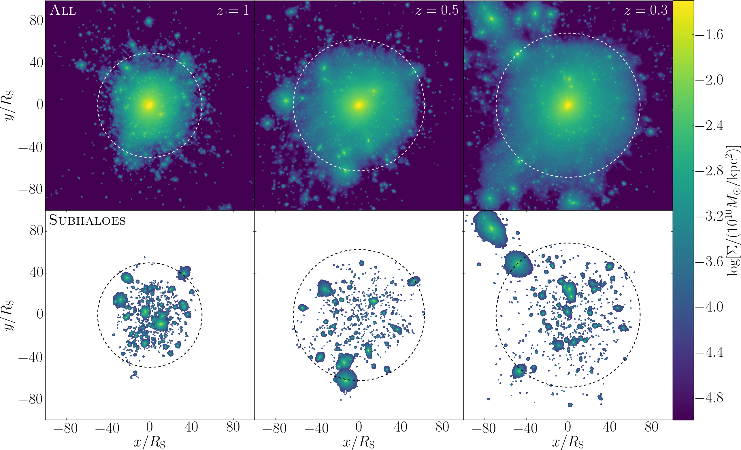
Figure 1: Column density of the dark matter in the Phase-1 simulation in the $x-y$ plane at $z=1$, $z=0.5$ and $z=0.3$, from left to right, respectively. Top row: the column density of all dark matter particles. Bottom row: the column density of subhaloes only. Total mass of the main halo and its subhaloes increases from $1.35\times 10^{11}\,\mathrm{M_{\odot}}$ to $2.29\times 10^{12}\,\mathrm{M_{\odot}}$ from $z=1$ to $z=0$, while the number of subhaloes changes from $893$ to $1083$. Dashed circles indicate the virial radius at these three epochs. The spatial coordinate is in the unit of the scale length of the disc $R_{\mathrm{S}}=3.13\,\mathrm{kpc}$.

The smooth component can be represented by the sum of a spherical and a triaxial part. Density profile of the spherical part, $\rho_{\mathrm{S}}(r)$, is constructed by spherically averaging the smooth component. We fit it with three Einasto profiles joined together (see left panel of Figure 12 and Appendix A). Compared to the dark matter halo profile in the original Aquarius simulation, our profile is more contracted in the centre due to the disc potential. Our disc model has a relatively low mass ($\sim 1\%$) compared to the main halo. This is to ensure that the effects due to self-gravity is suppressed, so that we can focus on the impact of external perturbations. The influence of the disc would be higher with a higher mass model. Following Bowden et al. (2013) and Hu & Sijacki (2016) the triaxial part is represented by two spherical harmonic functions, aiming to reproduce our desired axis ratio profile. The axis ratio profile of the smooth component in our simulation is calculated following a similar method to Vera-Ciro et al. (2011), where we iteratively compute the eigenvalues and eigenvectors of the “reduced” inertia matrix of an ellipsoid of a certain radius. We find that the axis ratio of the smooth component significantly fluctuates as a function distance from the centre and is rather triaxial in the centre (see solid curves in the right panel of Figure 12). This occurs as we only introduce a stellar disc to modify the dark matter halo shape and do not consider larger scale contribution from stars or gas. This would make the disc very elliptical and unstable. To avoid this issue, we impose a much smoother halo shape variation with radius (see dashed curves in the right panel of Figure 12), where the outer axis ratios are comparable to those obtained from our Phase-1 simulation.

Having computed $\rho_{\mathrm{S}}(r)$ and the axis ratios in $x-y$ plane, $p(r)$, and in $x-z$ plane, $q(r)$, we can calculate the density profile of the triaxial part as follows

$$\rho_{\mathrm{T1}}(r)=\left(1-\frac{3q(r)^{\alpha}}{1+p(r)^{\alpha}+q(r)^{\alpha}}\right)\rho_{\mathrm{S}}(r)$$ (2)

and

$$\rho_{\mathrm{T2}}(r)=\frac{1}{2}\frac{1-p(r)^{\alpha}}{1+p(r)^{\alpha}+q^{\alpha}}\rho_{\mathrm{S}}(r),$$ (3)

where $\alpha=-\mathrm{d}\log\rho_{\mathrm{S}}(r)/\mathrm{d}\log r$ is the slope of the spherically averaged density profile. We enclose a brief explanation of these formula in Appendix B. Hence, the total density profile of the halo is

$$\rho(r,\theta,\varphi)=\rho_{\mathrm{S}}(r)-\rho_{\mathrm{T1}}(r)Y_{2}^{0}(\theta)+\rho_{\mathrm{T2}}(r)Y_{2}^{2}(\theta,\varphi),$$ (4)

whose potential can be then integrated numerically using the Green’s function, as shown in Appendix C.

2.3 Phase-2: Introducing a Live Disc in a Static, Triaxial Dark Matter Halo Potential

The stellar disc is setup initially following Equation (1) and has $10^{6}$ stellar particles. The total mass of the halo inside $5R_{\mathrm{S}}$ is $\sim 1.6\times 10^{11}M_{\odot}$, while the mass of the disc inside $5R_{\mathrm{S}}$ is $\sim 9\times 10^{9}M_{\odot}$. The dynamics of the central disc is therefore dominated by the dark matter halo as expected. Due to the high-$Q$ profile of the stellar disc, the swing amplification is weak. We therefore do not need higher number of particles to prevent transient gravity-induced spiral structures from forming (for further details see Hu & Sijacki, 2016). The stellar disc is initially in equilibrium with a spherical halo, and as shown in Hu & Sijacki (2016) it will develop strong two-armed spirals if we put it directly into our smooth triaxial dark matter halo model. To avoid such structures and focus on the effect of subhaloes alone we have to evolve the disc inside a dark matter halo that changes adiabatically from spherical to triaxial. We change the halo in a way similar to Section 3.3 in Hu & Sijacki (2016). Namely, we start the simulation with the spherical part of the halo only, while the triaxial part of the halo grows adiabatically with time, where the total potential of the halo is

$$\Phi(r,\theta,\phi)=\Phi_{\rm S}(r)+f(t)\Phi_{\rm T}(r,\theta,\phi)\,.$$ (5)

Here $\Phi_{\rm S}$ is the static spherical part, $\Phi_{\rm T}$ is the triaxial part and the growth factor $f(t)$ changes from $0$ to $1$ following

$$f(t)=(1-\frac{1}{6}\mathrm{e}^{-t/\tau_{\mathrm{I}}}(1+5\mathrm{e}^{-t/\tau_{\mathrm{I}}}))^{6}\,,$$ (6)

where we have set timescale $\tau_{\mathrm{I}}=1\,\mathrm{Gyr}$ as in our previous work. We evolve the system for $5\,\mathrm{Gyr}$ and find no prominent structures in the disc. The surface density of the final stellar disc is shown in the top left panel of Figure 4.

2.4 Phase-3: Simulating Live Stellar Disc in Static Triaxial Dark Matter Halo with Live Subhaloes

With the halo and the disc setup in Phase-1 and Phase-2, we are now able to perform our final simulation starting from $z=1$ that studies the influence of subhaloes on the stellar discs. In this simulation, three components are included:

• A static, triaxial dark matter potential. We include it rather than live dark matter particles because it will save considerable computational resources and more importantly it will not induce numerical perturbations in the disc due to the Poisson noise (note that due to very different spatial scales of the disc and the halo, dark matter particle mass would need to be considerably larger than the disc particle mass), thus making it much more robust to study the influence of subhaloes only. Including a static dark matter potential rather than a live dark matter halo may however create an artificial torque, as in reality the main dark matter halo should gravitationally respond to the impacting subhaloes as well. As discussed in detail in Appendix D, we estimate the upper limit on this effect and find that it is overall weaker than or at most comparable to the genuine effect of subhaloes for $m=1$ modes, and negligible for $m=2$ modes.

• Live subhaloes. The live subhalo particles are taken directly from the Phase-1 simulation at $z=1$. As mentioned earlier, they consist of particles that are gravitationally bound to any subhalo of our main halo at $z=1$ or at any later time, based on the subfind algorithm. In this way we ensure that there is a realistic number of subhaloes during the whole period of the Phase-3 simulation. We have in total 2,035,019 live dark matter particles included, each having a mass of $m_{\mathrm{DM}}=3.93\times 10^{5}\,\mathrm{M_{\odot}}$.

• A live disc. The live disc is taken from the Phase-2 simulation at $5\,\mathrm{Gyr}$. As explained above, it is in equilibrium with the triaxial dark matter potential, and no prominent spiral structures exist in the disc.

3 Results

3.1 Properties of Subhaloes that Interact with the Disc

Figure 2: Distribution of dark matter in $x$-$y$ plane (left) and $x$-$z$ plane (right). Plots in the top row show the column densities of all dark matter particles at $z=1$. Plots in the middle row show the column densities of all subhalo particles in the inner halo region at $z=1$. Different letters indicate the initial position of different subhaloes which interact with the disc at a later time. Plots in the bottom row show the trajectories of the subhaloes that interact with the disc (see Table 1). In particular, subhaloes A and C are the same subhalo hitting the disc at two different redshifts, so are subhaloes B and E. The location of subhaloes at the time of impact is marked with crosses, while location at $100\,\mathrm{Myr}$ before and after the impact is marked with diamonds and at $200\,\mathrm{Myr}$ with squares. The column density of the stellar disc is also shown in the bottom row for comparison.

Table 1: Subhaloes that interact with the disc in the Phase-3 simulation. Redshift of maximum mass before the impact, $z_{\max{}}$, maximum mass before the impact, $M_{\mathrm{sub}}$, half-mass radius at the time of maximum mass before the impact, $R_{\mathrm{hm}}$, redshift of impact, $z_{\mathrm{i}}$, radius of impact, $R_{\mathrm{i}}$, the angle of incidence, $\theta_{\mathrm{in}}$ and the rotation direction is listed. The half-mass radius and the impact radius is shown in units of the scale length of the disc, $R_{\mathrm{S}}=3.13\,\mathrm{kpc}$. The angle of incidence is defined as the angle between the trajectory and the normal direction of the disc. When $\theta_{\mathrm{in}}>90$, the subhalo hits the disc from below. For rotation direction, “R” stands for retrograde, while “P” stands for prograde.

id	$z_{\max{}}$	$M_{\mathrm{sub}}$	$R_{\mathrm{hm}}$	$z_{\mathrm{i}}$	$R_{\mathrm{i}}$	$\theta_{\mathrm{in}}$	rotation
		[$10^{10}\,\mathrm{M_{\odot}}$]	$/R_{\mathrm{S}}$		$/R_{\mathrm{S}}$		direction
A∗	1.22	1.63	1.28	1.02	1.81	57	R
B	0.99	0.37	1.85	0.87	2.19	132	R
C	0.95	0.53	1.28	0.80	0.70	129	R
D	0.76	0.14	1.93	0.46	2.12	165	P
E	0.80	0.12	1.57	0.42	1.63	44	P
F	0.46	0.13	1.20	0.37	2.85	78	P
G†	0.47	4.8	6.39	0.39	-	-	P

^∗At the start of the simulation, subhalo A is very close to the disc and moving away from it. Based on its velocity we estimate that it hits the disc at $z=1.02$.

^†As shown in Figure 2, subhalo G moves through the disc plane about $10\,R_{\mathrm{S}}$ away from the disc centre, therefore it is not considered as a close impact. However, thereafter subhalo G flies over the disc, largely parallel to it, at a distance of less than $3\,R_{\mathrm{S}}$, which has a substantial influence on the disc. We therefore include subhalo G in this table but omit its impact radius and the angle of incidence. The impact redshift $z_{\mathrm{i}}$ is defined as the redshift when subhalo G is closest to the centre of the main halo.

The column density of dark matter at $z=1$ is shown in the top row of Figure 2. Outside of the main halo there is a large number of subhaloes that may fall in at a lower redshift. A zoom-in view of the column density of all subhaloes in the Phase-3 simulation at $z=1$ is shown in the middle row of Figure 2. From all these subhaloes we select the ones that interact with the disc based on the following criteria: a) their impact radius $r$ is less that $5\,R_{\mathrm{S}}$, b) their mass exceeds $10^{9}\,\mathrm{M_{\odot}}$. There are more subhaloes that either hit the disc plane further out or have a lower mass, but we filter them out as they play a minor role in the development of spiral structures in the disc as we have explicitly checked (see e.g. Appendix E). The properties of impacting subhaloes based on our criteria above are listed in Table 1. They hit the disc at various redshifts from $z=1$ to $z\sim 0.4$ and have different angle of incidence and rotation direction. Generally, as expected, subhaloes that are further away from the centre of the halo hit the disc at a lower redshift. We indicate their initial locations at $z=1$ in the first two rows of Figure 2 with different letters, and we plot their trajectories once close to the disc in the bottom row of Figure 2, along with the column density of the disc.

The impact radius $R_{\mathrm{i}}$ is typically between $0.7R_{\mathrm{S}}$ and $2.9R_{\mathrm{S}}$. The half-mass radius of the subhaloes at the time of maximum mass before the impact is lower than the impact radius for all subhaloes except for subhalo C and G, for which $R_{\mathrm{hm}}$ and $R_{\mathrm{i}}$ are comparable. However, note that at the time of impact, the half-mass radius decreases to $10$-$40\%$ of its maximum value before the impact as a result of tidal stripping, which means that at the time of impact, the subhaloes should be considered as objects of relatively small size. It is therefore a reasonable estimate to consider an impacting subhalo in our simulation as a point mass.

A closer look at each subhalo reveals that there are in fact only 5 subhaloes in the 7 subhalo events, as subhalo A and C are the same subhalo hitting the disc twice, so are subhaloes B and E. It is also worth noting that subhalo A does not hit the disc during the Phase-3 simulation. It goes through the disc at $z=1.02$, before the beginning of the Phase-3 simulation, and at the start of Phase-3, it is located very close to the disc, moving away from it. Subhalo G does not hit the disc within $5\,R_{\rm S}$, but crosses the disc plane further away from the disc centre. However, it is very close to the disc at $z\sim 0.4$ passing over the disc at a distance of no more than $3\,R_{\rm S}$, as shown by the black curve in the bottom row of Figure 2.

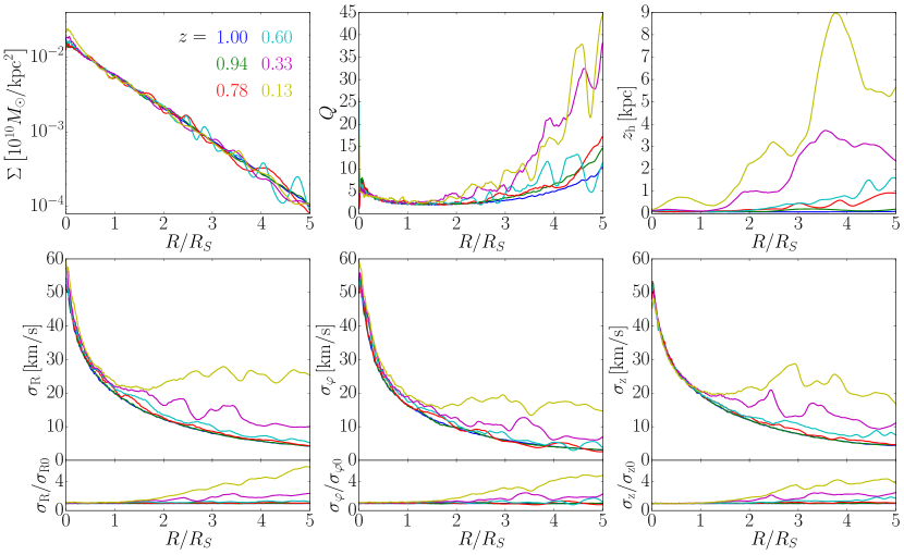
Figure 3: The time evolution of disc’s surface density, $\Sigma$, Toomre’s $Q$ parameter, disc thickness, $z_{\mathrm{h}}=\sqrt{\left\langle z^{2}\right\rangle-\left\langle z\right\rangle^{2}}$, and velocity dispersion in the radial, azimuthal and vertical direction, $\sigma_{\rm R}$, $\sigma_{\rm\varphi}$ and $\sigma_{\rm z}$, respectively. The surface density of the disc fluctuates in the outer region and increases somewhat in the innermost region at later times. The Toomre’s $Q$ parameter increases significantly in the outer region, i.e. for $R\gtrsim 2R_{\rm S}$, which can be explained by the increase of $\sigma_{\rm R}$. Disc also thickens considerably in the outer region after $z=0.5$. Aside from thickening, we find strong warps in the disc after $z=0.5$.

As mentioned in Section 2.4, an analytic dark halo potential is employed in the Phase-3 simulation instead of a live dark matter main halo. To study its influence on the subhaloes and understand if it is biasing our results in any way, we compared the mass loss and trajectory of each subhalo listed in Table 1 in the Phase-3 simulation with its counterpart in the Phase-1 simulation, where a live main halo is present (but not a live stellar disc). We find that the mass loss of each subhalo at the moment of impact is similar between the two simulations, ranging from $50\%$ to $80\%$ (for further details see Appendix F). The mass loss is mainly induced by tidal disruption in both simulations. We also note that due to dynamical friction, the subhaloes in the Phase-1 simulation move slower than those in the Phase-3 simulation, which delays the time of the impact by up to $1\,\mathrm{Gyr}$, but subhaloes have comparable velocities at impact and spend similar amounts of time in the vicinity of the disc. Therefore, with respect to the properties of subhaloes, using an analytic main halo potential instead of a live dark matter main halo should not affect our results below.

3.2 Disc Heating in Response to Subhaloes

As the subhaloes interact with the disc its properties change, as shown in Figure 3, especially at later times when the massive, fly-by subhalo G interacts with the disc. The spherically averaged surface density of the disc (top left panel) fluctuates in the outer region due to strong spiral and ring structures caused by subhaloes. In the innermost region, the density of the disc grows mildly at later times as a bar gradually forms. Top middle panel shows the radial profile of Toomre’s $Q$ parameter which is defined as

$$Q=\frac{\sigma_{\rm R}\kappa}{3.36\,G\Sigma}\,,$$ (7)

where $\sigma_{\rm R}$ is the velocity dispersion in the radial direction, $\kappa=\frac{2\Omega}{R}\frac{\mathrm{d}}{\mathrm{d}R}(R^{2}\Omega)$ is the epicyclic frequency (with $\Omega$ being the rotation angular velocity of stars), $G$ is the gravitational constant and $\Sigma$ is the surface density. Toomre’s $Q$ parameter quantifies how strong the swing amplification is in the disc. We found in Hu & Sijacki (2016) that the disc is stable to swing amplification of the Poisson noise when $Q>1.3$ throughout the disc, thus we ensure this is the case for our initial setup (see blue curve at $z=1$).

In our Phase-3 simulation Toomre’s $Q$ parameter increases in the outer region of the disc after $z\sim 0.5$, which can be explained by the significant increase of the velocity dispersion in the radial direction, $\sigma_{\rm R}$, shown in the bottom left panel of Figure 3. The velocity dispersion in the other two directions, $\sigma_{\rm\varphi}$ and $\sigma_{\rm z}$, also increases similarly (see bottom middle and right panels). This is caused by the interaction of the disc with subhalo G, as we will discuss in detail in Section 3.6.

We quantify the thickness of the disc, $z_{\rm h}$, by computing the standard deviation of the $z$ coordinate of stellar particles, i.e. $z_{\rm h}=\sqrt{\left\langle z^{2}\right\rangle-\left\langle z\right\rangle^{2}}$. We find that the fly-by subhalo G leads to strong warps in the disc, which causes the disc thickness, $z_{\rm h}$, to increase significantly at later times, as shown in the top right panel of Figure 3. Further smaller mass subhaloes interact with the disc in the wake of subhalo G which increases the disc thickness further from $z=0.33$ to $z=0.13$.

Moetazedian & Just (2016) studied this heating effect with re-simulations of Aquarius and Via Lactea haloes with Milky Way-like discs. Compared to their results, we find similar ring-type density fluctuations. The disc thickening and heating rate before $z=0.5$ is moderately higher than found by Moetazedian & Just (2016), which could be due to the fact that our stellar disc is less massive. For $z<0.5$, we see much higher disc thickening and heating due to the massive subhalo G, which, interestingly, has a similar mass to a massive subhalo in their Aq-F2 model (both $\sim 5\times 10^{10}$), which also caused a significant jump in disc thickness and velocity dispersion. Furthermore, similarly to Moetazedian & Just (2016), all of the examined disc properties are affected by the subhaloes primarily in the outer regions, while in the innermost disc region, i.e. for $R<2\,R_{\rm S}$, these global disc properties change much less. This is not the case for the modes triggered in the disc which we discuss in the section below.

3.3 Modes in the Disc Triggered by Subhaloes

The interaction of subhaloes with the stellar disc leads to the development of spirals, rings and bars. Figure 4 shows the time evolution of the surface density (top panels) and the residual surface density (bottom panels) from $z=1$ to $z=0.13$. By construction, the disc is free of spiral structures at $z=1$ and it is slightly elliptical due to the triaxial dark matter halo. Thereafter, at least three distinct episodes of single-armed spiral structures appear in the disc: one shortly after the beginning of the simulation, one at $z\sim 0.78$, and one at $z\sim 0.33$. These single-armed spiral structures are counter-rotating and leading (with respect to the direction of the galactic rotation), which we study in detail in Section 3.4. Two-armed spiral structures also develop in the disc and are clearly visible when the single-armed spirals wind up, namely at $z\sim 0.60$ and at $z\sim 0.13$. Both single-armed and two-armed spiral structures extend from the centre of the disc to the edge of the disc when fully developed. While disc remains largely axisymmetric during most of the simulated time, at $z\sim 0.33$ the interaction with the very massive subhalo G causes warps, rings, and lopsidedness in the disc, and the formation of the central bar. At lower redshifts, spirals wind up and weaken and the disc then evolves towards a more axisymmetric and quasi-stable state. Note that the strength of different modes in the disc can be quite high, especially in the outer regions, as can be seen from the bottom panels, and we turn to quantify this next.

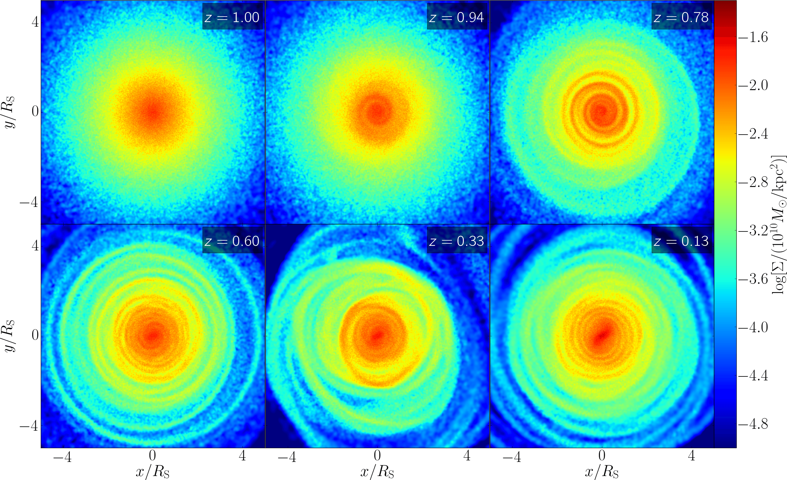
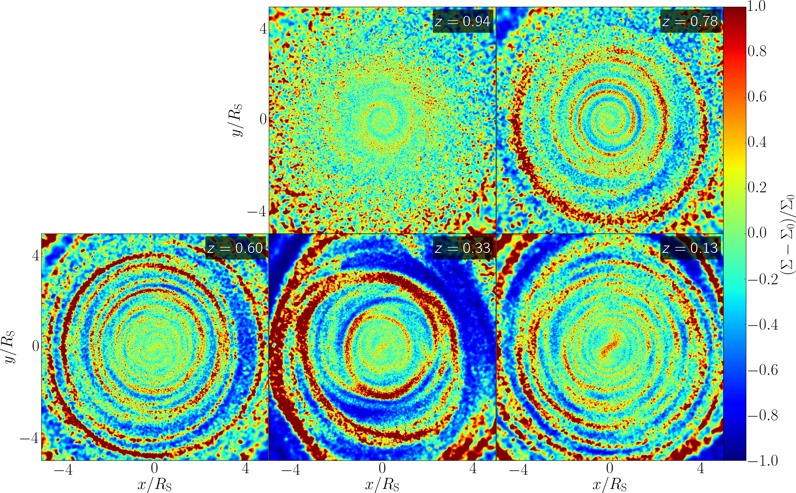
Figure 4: The evolution of the surface density $\Sigma$ (top panels) and the normalized residual surface density $(\Sigma-\Sigma_{0})/\Sigma_{0}$ (bottom panels) at different redshifts, where $\Sigma_{0}$ is the surface density at $z=1$. Single-armed spiral structures develop very quickly in the disc centre and they are counter-rotating and leading (i.e. the outer tip points towards the direction of the galactic rotation). These initial spiral structures wind up over time as the second episode of spirals forms in the disc at $z=0.78$. Newly formed single-armed spiral structures wind up as well and become weaker at $z=0.60$, when the two-armed spiral structures start to become apparent in the disc centre. The disc stays quiet for a while until $z=0.33$, when a strong perturbation by subhalo G disturbs the disc in the outer region. This significantly warps the disc and generates the central bar. For $z<0.2$ spirals wind up and weaken. The disc recovers to a quasi-stable state overtime and at $z=0.13$, two-armed spiral structures are visible again in the central region of the disc.

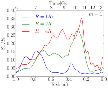
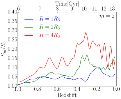
Figure 5: Strength of the modes in the disc as a function of time evaluated at $1$, $2$ and $4\,R_{\rm S}$ for $m=1$ modes (left panel) and $m=2$ modes (right panel). Here the relative strength $S_{m}/S_{0}$ is shown, where $S_{m}$ is defined in equation (8). $S_{0}$, the strength of $m=0$ modes, is the spherically averaged surface density at radius $R$ by definition. For the $m=1$ case, multiple generations of modes are triggered over time, first one at $z\sim 1$, second one at $z\sim 0.78$, and third one at $z\sim 0.33$. Distinct generations of modes can be better identified in the inner than the outer region, as the winding time for the inner region is much shorter such that the different generations of modes do not interact significantly. The third generation of modes is also prominent in the $m=2$ case.

The time evolution of the strength of $m=1$ (left panel) and $m=2$ (right panel) modes is shown in Figure 5. Here the strength of the modes is the relative strength of the Fourier transform of the surface density $\Sigma(R,\theta)$ of the disc over the azimuthal coordinate $\theta$, i.e.,

$$S_{\rm m}(R)=\left|\frac{1}{2\pi}\int_{\mathrm{-\pi}}^{\pi}\Sigma(R,\theta)e^{-im\theta}d\theta\right|\,,$$ (8)

where $m$ is the number of folds of the structure. For $m=0$, $S_{m}$ is simply the average surface density of a ring in the stellar disc at radius $R$. As expected, the evolution of $m=1$ modes at $R_{\rm S}$ correlates with Figure 4 very well, showing three distinct episodes of modes from $z=1$ to $z=0$. The estimated life time for each of the three episodes of spirals, measured by the full width at half maximum, is $\sim 1\,\mathrm{Gyr}$. Therefore, to have persistent single-armed spirals in the stellar disc, there should be every few Gyr massive enough subhaloes hitting the stellar disc. For the outer region of the disc at $2R_{\rm S}$ and $4R_{\rm S}$, similar generations can also be found, but less distinctively. This is because: a) more (smaller) subhaloes hit the outer region of the disc, leading to a noisier evolution history of the mode strength, and b) the life time of each episode of modes is longer due to the much lower winding rate, as shown later in Section 3.4. $m=2$ modes generally have lower strength and are less distinctive, due to their even slower winding rate. Nevertheless, strong $m=2$ modes are generated at $z\sim 0.35$, corresponding to the third episodes of $m=1$ modes. We will explore the connection between different modes generated in the disc and individual subhaloes in Section 3.5.

3.4 Nature of the Spiral Structures

We now turn to study the nature of the spiral structures by looking at their power spectra. As explained in detail in Hu & Sijacki (2016), the power spectra of the stellar disc are the Fourier transforms of the disc’s surface density over time and the azimuthal coordinate. The power spectra of the density field are typically plotted in the pattern speed-radius plane for each mode. If the power contour follows the Lindblad resonance, the spiral structures are kinematic density waves (Lindblad, 1963), while if the power spectra show patterns of horizontal bars between the inner and outer Lindblad resonance, the spiral structures are related to self-gravity (Sellwood & Carlberg, 2014).

The power spectra of our stellar disc in the Phase-3 simulation are shown in Figure 6. Here we plot the power spectra for $m=1$ (left panels) and $m=2$ (right panels) modes for the redshift ranges of $0.5<z<1$ and $0<z<0.5$. The first redshift range corresponds to the first two episodes of spirals, while the second redshift range corresponds to the third episode of spirals.

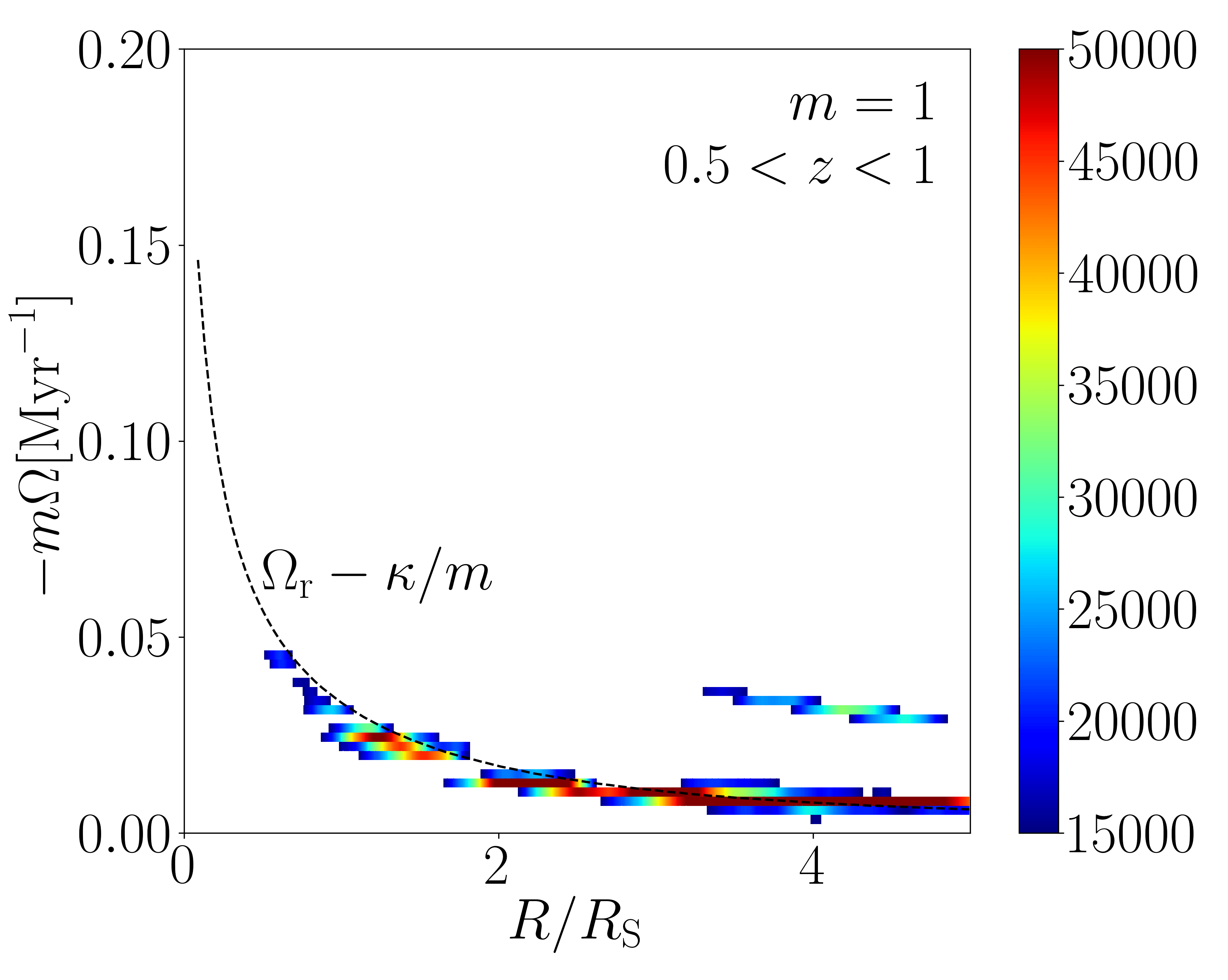
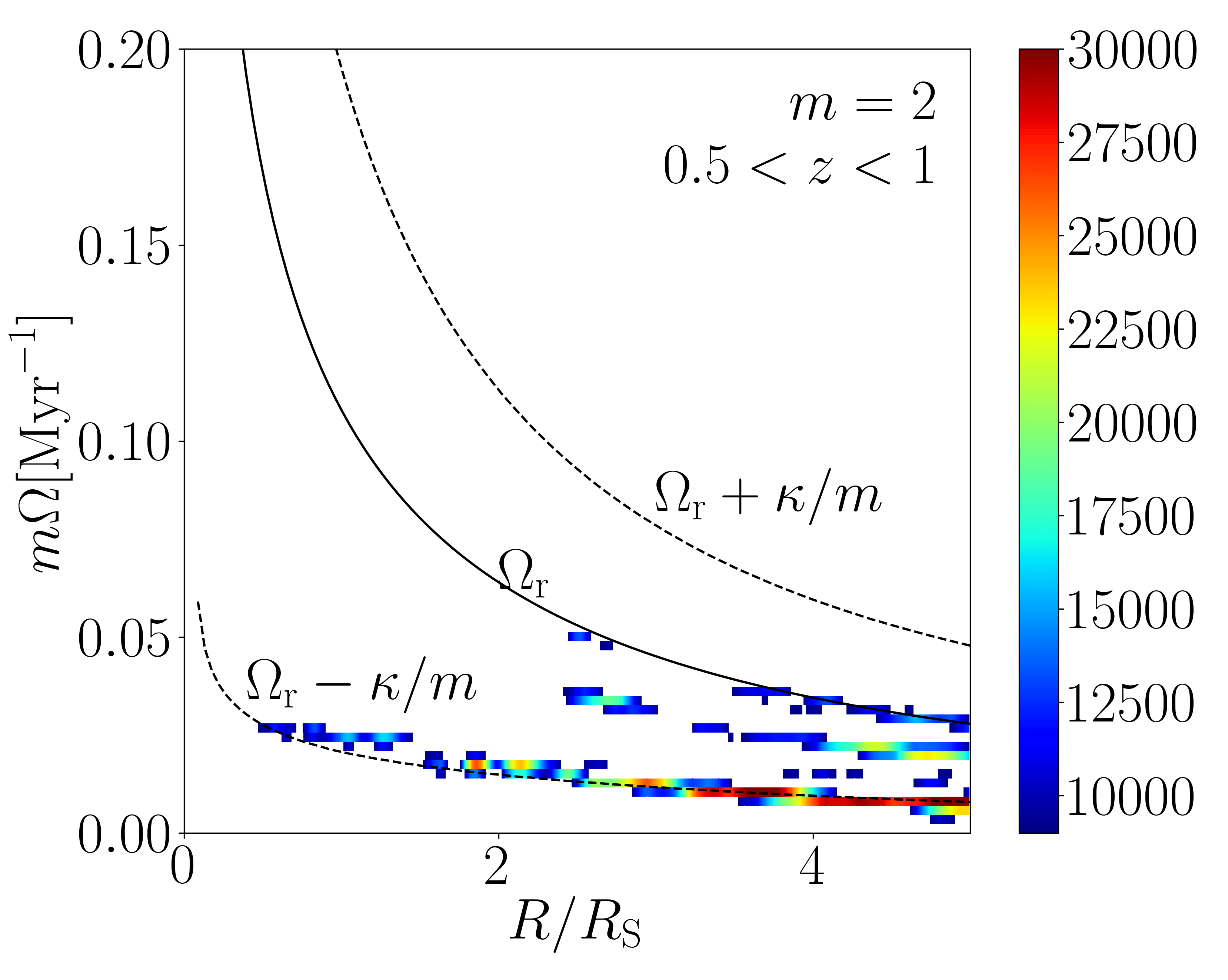
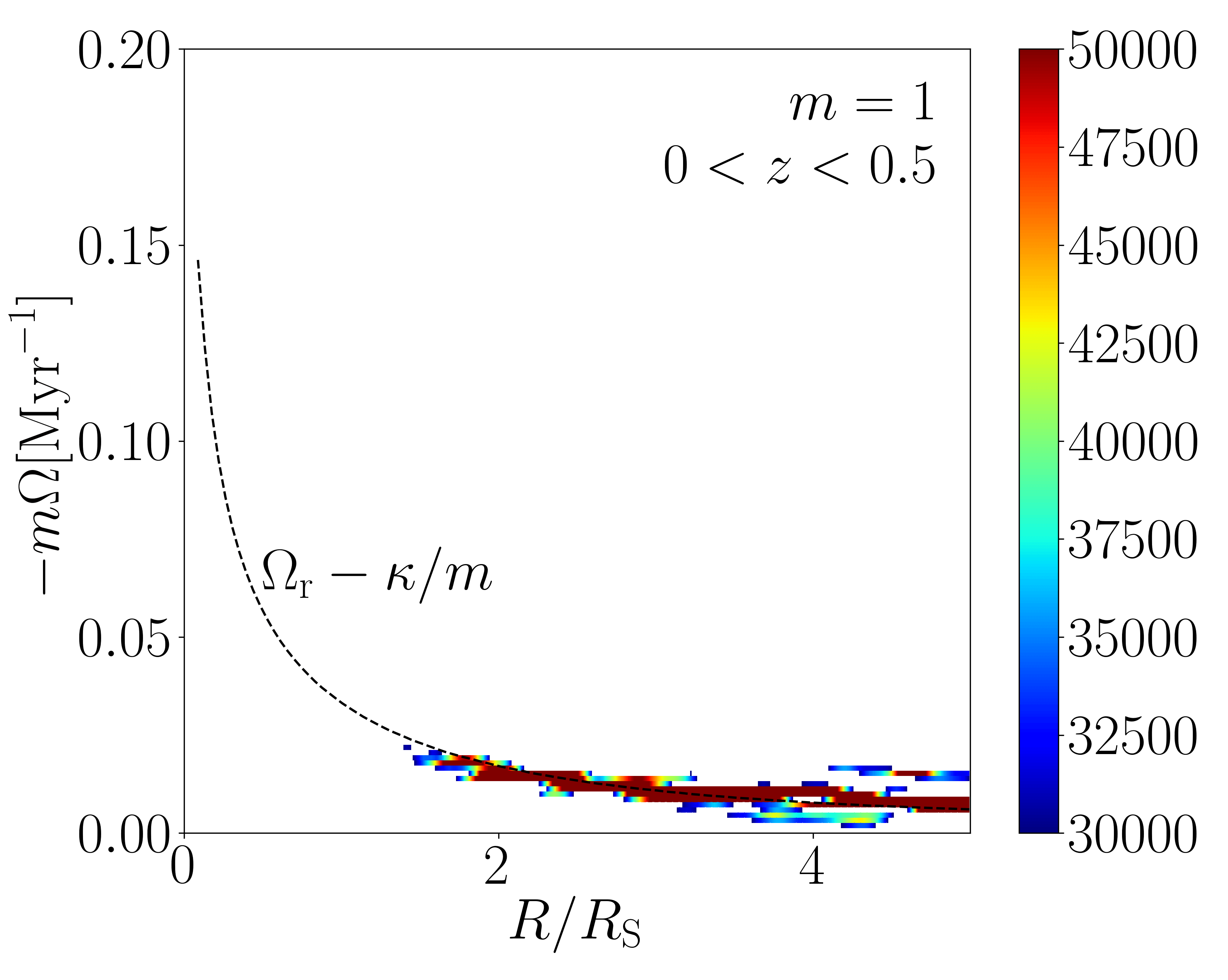
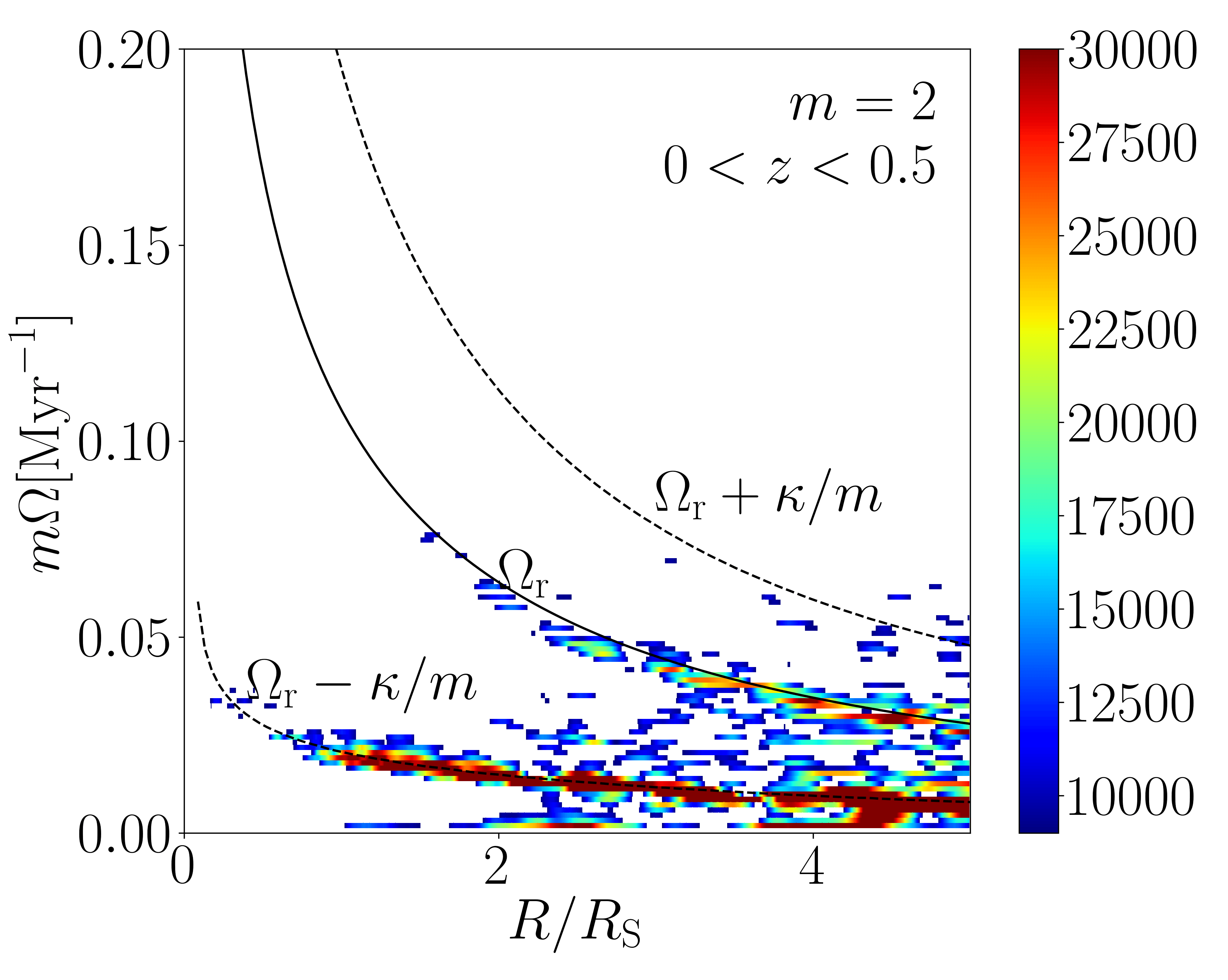
Figure 6: Power spectra of the $m=1$ (left panel) and $m=2$ (right panel) modes for the time intervals from $z=1$ to $z=0.5$ (top panels) and from $z=0.5$ to $z=0$ (bottom panels). For $m=1$ modes, the power of rotating patterns is shown in the $-m\Omega$-$R$ plane, where $-m\Omega$ is negative pattern speed multiplied by the number of modes $m$ and $R$ is the radius from disc centre. For $m=2$ modes, the power is shown in the $m\Omega$-$R$ plane. The co-rotation curve $\Omega_{\rm r}$ is plotted with a solid curve, while the Lindblad resonances $\Omega=\Omega_{\rm r}\pm\kappa/m$ are plotted with dashed curves, where $\Omega_{\rm r}$ is the rotating speed of stars and $\kappa$ is the epicyclic frequency. It can be seen that power spectra follow closely the inner Lindblad resonance both for $m=1$ and $m=2$ modes, indicating the kinematic density wave nature of the modes. The power of patterns between $z=0.5$ and $z=0$ is stronger than that between $z=1$ and $z=0.5$, which agrees with Figure 4 and 5.

We plot the power for $m=1$ modes in negative pattern speed because the single-armed spirals are found to be counter-rotating (i.e. to have negative pattern speed). In fact, the inner Lindblad resonance $\Omega_{\rm r}-\kappa/m$ is also negative for $m=1$ modes. As shown in the left panels in Figure 6, at all radii the highest power follows closely the inner Lindblad resonance, indicating that the modes in the disc are indeed kinematic density waves. We should always expect grand-design single-armed spiral structures of this kind to be counter-rotating as long as $\kappa>\Omega_{\rm r}$.

For $m=2$ modes, the power spectra are weaker than in the case of $m=1$ modes, in agreement with Figure 5. The highest power of $m=2$ modes also follows the inner Lindblad resonance closely. There are other weaker powers away from the inner Lindblad resonance, which should be relevant to other weaker resonances. The winding rate of spiral structures depends on the slope of the Lindblad resonance curve, which is much steeper for $m=1$ modes than the generally flat inner Lindblad curve for $m=2$. This explains why the life time of the single-armed spiral structures, typically less than $2\,\mathrm{Gyr}$, is lower than the life time of two-armed spiral structures studied in Hu & Sijacki (2016).

The winding rate difference also explains the inside-out fashion of spiral formation. As shown in Figures 4 and 5, most spiral structures in our simulation form first in the inner region and then “grow” towards the outer regions. To illustrate this, we calculate the slope of the pattern speed for $m=1$, at $1R_{\mathrm{S}}$, $\mathrm{d}\Omega_{\mathrm{P}}/\mathrm{d}R=0.0283\mathrm{Myr^{-1}}R_{\mathrm{S}}^{-1}$, while at $2R_{\mathrm{S}}$, the slope is $\mathrm{d}\Omega_{\mathrm{P}}/\mathrm{d}R=0.0092\mathrm{Myr^{-1}}R_{\mathrm{S}}^{-1}$. The changing rate of the tangent of the pitch angle $\alpha$ is

$$\frac{\mathrm{d}\tan\alpha}{\mathrm{d}t}=R\frac{\mathrm{d}\Omega_{\mathrm{P}}}{\mathrm{d}R}\,.$$ (9)

Therefore, the tangent of the pitch angle changes about $53\%$ faster at $1R_{\mathrm{S}}$ than that at $2R_{\mathrm{S}}$. For comparison, it takes $\sim 0.7\mathrm{Gyr}$ for spiral structures at $1\,R_{\mathrm{S}}$ to develop with tripled-mass subhalo B (mentioned later in Section 3.5 and Figure 8), while at $2\,R_{\mathrm{S}}$, it takes $\sim 1.2\mathrm{Gyr}$, about $71\%$ longer. This explains why spiral structures in the inner region develop faster and fade out faster.

In combination with Figure 4 which demonstrates that two-armed spiral structures become prominent almost always after the winding of single-armed spirals, we conclude that subhaloes trigger both $m=1$ and $m=2$ modes in the disc simultaneously, but with $m=1$ modes initially stronger than $m=2$ modes. In the inner disc, the winding rate of the $m=1$ modes is much faster than that of the $m=2$ modes, leading to a much quicker decrease of the strength of the $m=1$ modes. $m=2$ modes, winding up much slower, become prominent after $m=1$ modes wind up.

We also search for the self-gravitating spiral modes for higher $m$ values. The typical strength of these modes is more than one magnitude lower than that of the kinematic modes. This is expected as the disc has high Toomre’s $Q$ parameter.

3.5 The Impact of Each Halo

We now aim to establish a direct link between different modes generated in the disc and the individual subhaloes that interact with the disc. We start by studying the first generation of modes (i.e. $0.85<z<1$). These modes develop immediately after the simulation starts, which is the time when subhalo A is very close to the disc centre. As mentioned in Section 3.1, subhalo A is moving away from the disc at the start of the simulation. To study the relation between subhalo A and the first generation of modes, we restart the Phase-3 simulation with the subhalo A removed.

To modify the mass of subhalo A and other subhaloes, we adopt the following procedure. We first find the most bound particle of the subhalo at the time of impact. The tidal stripping does not influence the inner core of the subhalo significantly, so this most bound particle always belongs to the same subhalo as we have explicitly verified. We trace this particle and hence the subhalo backwards in time to find the redshift where the subhalo has the maximum mass before the impact. This usually is the time when the subhalo is furthest away from the main halo. We find all particles belonging to the subhalo at this redshift, and change their mass in the initial conditions. We then restart the simulation to see the impact of changed mass.

As highlighted by the light blue region in Figure 7, when the subhalo A is removed, $m=1$ modes before $z=0.85$ at $1\,R_{\rm S}$ seen in the original simulation essentially no longer develop. For $R=2\,R_{\rm S}$ and $R=4\,R_{\rm S}$ we see similar decrease in mode strength, but compared to $R=1\,R_{\rm S}$, the influence of removing subhalo A persists longer because the winding rate of $m=1$ modes at $1\,R_{\rm S}$ is much higher than that of the outer region.

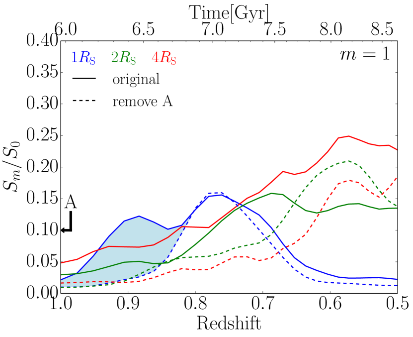
Figure 7: Comparison of the strength of the modes in the original simulation (continuous curves) and a simulation where subhalo A is removed (dashed curves). As highlighted with a light blue shade, when the subhalo A is removed, no prominent modes form between $z=1$ and $z=0.85$ at $1\,R_{\rm S}$. This is also true at $2$ and $4\,R_{\rm S}$, indicating that the first generation of modes is caused by the impact of subhalo A.

The second generation of modes at $1\,R_{\rm S}$ develops between $z\sim 0.87$ and $z\sim 0.6$, which coincides with the time of impact of subhaloes B and C. Recall that subhalo C is the same subhalo as A, whose influence on the second generation of modes can be studied with Figure 7. By removing subhalo A/C, the strength of the second generation of modes at $1\,R_{\mathrm{S}}$ reduces only slightly for $0.6<z<0.75$. To study the influence of subhalo B, we first restart the original simulation with subhalo B removed. The result is shown with the dashed curves in Figure 8. As highlighted by the light blue region in the left panel, the strength of the second generation of $m=1$ modes at $1\,R_{\rm S}$ decreases greatly when subhalo B is removed, while a mild decrease can be found at $2\,R_{\rm S}$. For $m=2$ modes, even though the original spiral strength is low, we can still find a mild decrease in the spiral strength once subhalo B is removed. Thus, the subhalo B is the main cause of the second generation of modes with the subhalo A/C contributing at a lower level.

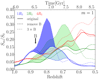
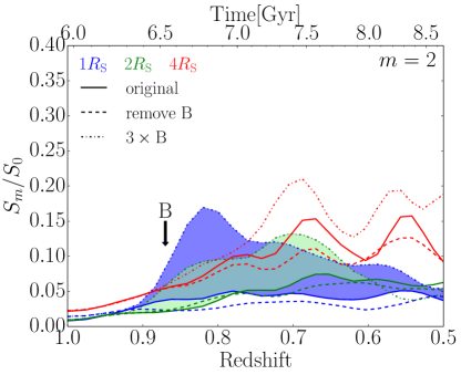
Figure 8: Comparison of the strength of the modes in the original simulation and simulations where either subhalo B (which hits the disc at $z=0.87$) is removed or its mass is tripled. When subhalo B is removed, the second generation of $m=1$ modes does not form at $1\,R_{\rm S}$, as highlighted by the light blue region, indicating that subhalo B is the main cause of these modes. When the mass of subhalo B is tripled, the strength of both $m=1$ and $m=2$ modes is increased, as highlighted by the dark blue region for $1\,R_{\rm S}$ and by the green region for $2\,R_{\rm S}$. Note that in the simulation with the tripled mass $m=2$ modes become dominant in central region for $z<0.75$ (see also Figure 9).

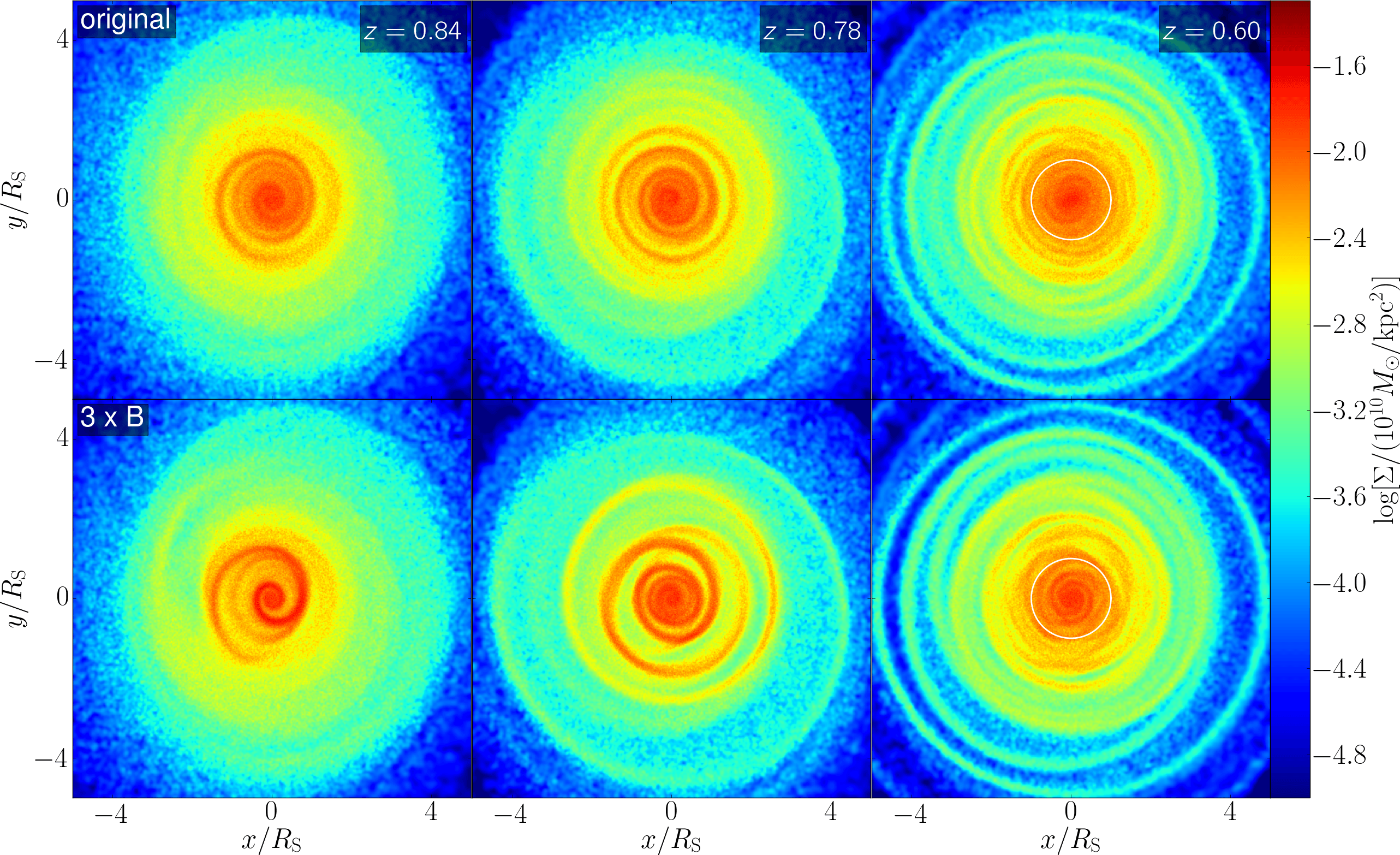
Figure 9: Surface density of the stellar disc in the original simulation (top panels) and the simulation where the mass of subhalo B is tripled (bottom panels). More massive subhalo B leads to very strong modes immediately after it hits the disc. Additionally to the spirals, strong ring structures also develop at $z=0.78$ in both simulations. When the single-armed spirals wind up at $z=0.60$, two-armed spiral structures become prominent in the disc centre, as highlighted by the white circles in the right panels. The two-armed spiral structures are more prominent when the mass of subhalo B is increased, in line with Figure 8.

Subhalo B starts from more than $40\,R_{\rm S}$ away from the disc centre and is mainly responsible for the second generation of modes, offering us a good test for studying the influence of subhalo properties, especially the subhalo mass, on the modes triggered in the disc. We hence find all dark matter particles that belong to subhalo B in the initial conditions, modify their mass, and restart the simulation. We run several simulations with different mass of subhalo B, including $1.5$, $2$ and $3$ times the original subhalo B mass. Note that to increase the mass of subhaloes we increase the mass of each particle in the simulation, which increases the gravitational force within the subhalo, resulting in a immediate shrinkage in the size of the subhalo. We argue that the shrinkage is acceptable because a) the maximum shrinkage in spatial scale is about $30\%$. At the time of impact, the half-mass radius is already small (typically less than $\sim 0.3\,R_{\mathrm{S}}$). The impact of the size change is therefore small; and b) we are more interested in the response of the disc to subhaloes of different mass, where the spatial scale of a subhalo plays a minor role.

The strength of modes when the mass of subhalo B is tripled is shown as dot-dashed curves in Figure 8 (other simulations with a lower subhalo B mass give consistent results which lie in between the original subhalo B mass and the tripled mass). We see a clear increase in mode strength for both $m=1$ and $m=2$ modes at $1\,R_{\rm S}$ (highlighted with the dark blue shade) and $2\,R_{\rm S}$ (highlighted with the green shade). We note that for $m=2$ modes, unlike in the original simulation, strong two-armed spiral structures now develop. This confirms that although the two-armed spiral structures are very weak in the original simulation, they are indeed triggered by the impact of the subhalo B. At $4\,R_{\rm S}$ the strength of modes also increases with the higher mass of subhalo B, and the influence remains for several Gyrs.

It is also worth noting that although both $m=1$ and $m=2$ modes at different radii start to develop at almost the same time, mode strength at $1\,R_{\rm S}$ always reaches its peak before that at $2\,R_{\rm S}$. This is caused by their different winding rate. When the mass of subhalo B is tripled, the second generation of $m=1$ modes reaches its peak strength $\sim 0.2\,\mathrm{Gyr}$ earlier than in the original simulation at $1\,R_{\rm S}$. We verify that when the mass is tripled, the trajectory of subhalo B does not change significantly. Instead, subhalo B interact with the disc earlier because its gravitational force field is stronger and can exert a torque on the disc earlier.

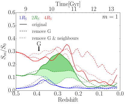
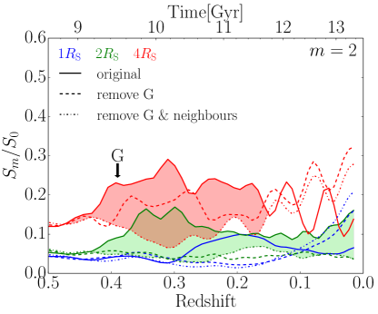
Figure 10: The strength of modes in the simulation where the fly-by subhalo G is removed. We either just remove subhalo G (dashed lines) or the surrounding subhaloes as well (dash dotted lines) which have similar starting positions and subsequent trajectories. The modes at $2\,R_{\rm S}$ are greatly reduced, as highlighted by the dark green region. When we remove the neighbouring subhaloes as well, the strength of the modes at $2\,R_{\rm S}$ and $4\,R_{\rm S}$ is reduced to a greater extend, as highlighted by the light green ($m=1$ and $m=2$) and the red ($m=2$) shaded regions. The strength of modes at $1\,R_{\rm S}$ is not effected significantly by the removal of subhalo G, but is caused by smaller mass subhaloes that interact with the disc.

The increase in the strength of both $m=1$ and $m=2$ modes is also illustrated in Figure 9, where a comparison of the surface density of the original simulation and of the simulation with 3 times subhalo B mass is shown. Similar to the original simulation, single-armed spiral structures are visible first in the simulation with the tripled mass, while two-armed spiral structures can be seen after the single-armed spiral structures wind up. At $z=0.84$, the single-armed spiral structures with tripled subhalo B mass are much more prominent than that in the original simulation, extending from the centre of the disc to $\sim 2\,R_{\rm S}$. The single-armed spiral structures propagate outwards from $z=0.84$ to $z=0.78$. $m=1$ modes soon wind up, and at $z=0.60$, very prominent two-armed spiral structures are in the centre of the disc. In the outer region, lopsided rings also form. This effect is similar to ring galaxies. As shown by Lynds & Toomre (1976), vertical impact of a massive point mass perturber can lead to such features. In fact, it has been shown with $N$-body simulations that energy kicks from minor mergers of satellites give rise to radial oscillation of various frequencies in the disc, leading to ringing in the disc and detectable phase warping in the velocity space (Quillen et al., 2009; Minchev et al., 2009; Gómez et al., 2012).

We also check that subhaloes A/C and B are indeed the main cause of all modes studied so far by removing both subhalo A and B. As shown in Figure 14, almost all modes are removed up to $z=0.7$. Though there are less massive subhaloes that hit the disc during this period, the evolution of the disc is dominated by these massive subhaloes only. We have similarly removed subhalo D, E and F, but no prominent change in spirals is found. We conclude the mass of these subhaloes is too small to have an appreciable effect. This is confirmed by an additional simulation (see Section 3.6), where we increase the mass of subhalo D by a factor of 10 and find that it causes spiral structures in the disc. It is worth noting that these less massive subhaloes have a small impact on spirals in our simulations, although their mass is larger than $10^{9}\,M_{\odot}$, the mass limit found by Pettitt et al. (2016). This may be due to the fact that Pettitt et al. (2016) set up simulations with only one subhalo at a time, while our simulations are much more dynamic with multiple subhaloes interacting at a time which can mask weak spirals.

3.6 Influence of the Fly-by Subhalo

As shown in Table 1 and in the bottom panels of Figure 2, subhalo G passes very close over the disc plane at $z\sim 0.39$ and as we have anticipated in previous sections it perturbs the disc significantly. We restart the original simulation with subhalo G removed to isolate its impact on the disc more clearly. As shown with dashed curves in Figure 10, the strength of the third generation of $m=1$ modes at $2\,R_{\rm S}$ decreases by more than $50\%$. However, unlike direct impacting subhaloes we studied so far, no prominent difference can be seen for $m=1$ modes at $1\,R_{\rm S}$ at $4\,R_{\rm S}$. For $m=2$ modes, strength at all radii decreases after removing subhalo G. When subhalo G is closest to the disc centre, its projection on the $x-y$ plane of the disc is $\sim 1.16\,R_{\rm S}$ away from the disc centre. As will be discussed later, the low strength of spirals in the inner region is related to the resonance effect. For $4\,R_{\rm S}$, the $m=1$ mode is not very effected because there are many more smaller subhaloes that interact with the outer region of the disc.

We notice that some $m=1$ and $m=2$ modes are still present in the disc when subhalo G is removed. We find that apart from the influence of the subhalo G, the third generation of modes also consist of: a) the remains of previously generated modes, b) structures generated by some smaller subhaloes hitting the disc, and c) modes triggered by “neighbours” of subhalo G that also fly over the disc at a similar time. To understand the interplay of these different effects, we remove all smaller subhaloes that hit the disc between $z=0.3$ and $z=0.5$. This removes the $m=1$ modes at $1R_{\rm S}$. As a second experiment, we remove subhalo G and its “neighbours”, i.e. subhaloes whose initial positions and trajectories are very similar to subhalo G’s. The strength of the modes at $2\,R_{\rm S}$ for $m=1$ and $2$ and $4\,R_{\rm S}$ for $m=2$ decreases further, as shown in the light green and red shaded regions in Figure 10. We therefore conclude that although subhalo G makes a crucial contribution to the third generation of modes, several other subhaloes also play a role.

3.7 Tidally-driven Spiral Structures

For all events, including direct subhalo impacts and the fly-by subhalo interaction, single-armed spiral structures form and dissolve before two-armed spiral structures are apparent. As explained in Section 3.4, the longevity of two-armed spirals depends on their flat inner Lindblad resonance curve. Further to this, we find that the interaction of each subhalo with the disc is more of an impulsive nature rather than determined by resonances.

Previous simulation works with a single perturber, e.g. Toomre & Toomre (1972); Howard et al. (1993) have found that prograde perturbers lead to $m=2$ spiral structures as the $m=2$ inner Lindblad resonance has a prograde speed (also see Sellwood (2012) and Fouvry et al. (2015) for the effect of resonance scattering during secular evolution of discs.) If subhaloes interact with the disc for a long time, resonances with the same pattern speed as the subhalo’s rotation angular velocity will have the strongest response. At a first glance this could be the case if we only consider subhaloes A and B. As shown in Table 1, subhaloes A and B are both retrograde. If they interact with the disc through resonances, modes with a negative pattern speed, i.e. $m=1$ modes, will be strongest, which agrees with our findings above (see also Athanassoula, 1978; Thomasson et al., 1989). However, we find that the typical rotational velocity of the subhaloes in our simulation is much higher than the typical pattern speed of $m=1$ and $m=2$ modes in the stellar disc. As a result, the interaction between subhaloes and the disc is rather impulsive, as we show next with a simulation with a massive prograde subhalo. In this simulation, we restart the Phase-3 simulation with the mass of subhalo D increased by a factor of $10$, where subhalo D is prograde. If the subhalo would interact with the disc through resonances, $m=2$ modes should be the strongest (because they have a positive pattern speed). However, we find that single-armed spiral structures still develop first and have a higher amplitude than the $m=2$ modes. This indicates that the explanation of resonances does not hold in our simulations.

Instead of resonances, we find that the strength of the spiral structures is more related to the strength of the torque exerted by the subhalo. The torque strength on the stellar disc at radius $R$ exerted by a subhalo is calculated in the following way. For each point on the trajectory of the subhalo, we calculate the gravitational force field $\mathbf{F}(\mathbf{r},t)$ of the subhalo, where $\mathbf{r}$ is the coordinate on the disc and $t$ is time. For simplicity we model the subhalo as a point mass. As mentioned in Section 3.1, the half-mass radius of subhaloes at impact is smaller than the impact radius, so the point mass model should be sufficient for the estimation of torque strength. We then calculate the torque field in normal direction of the disc $T_{\mathrm{z}}(\mathbf{r},t)$ as

$$T_{\mathrm{z}}(\mathbf{r},t)=\left[\mathbf{r}\times\mathbf{F}(\mathbf{r},t)\right]_{\mathrm{z}}.$$ (10)

To quantify the total torque exerted by a given subhalo over its whole trajectory, we integrate the $z$ component of the torque, $T_{\rm z}(\mathbf{r},t)$, of the subhalo over time to get

$$L(\mathbf{r})=\int_{t_{\rm 0}}^{t_{\rm f}}T_{\rm z}(\mathbf{r},t)\,\mathrm{d}t\,,$$ (11)

where $t_{\rm 0}$ and $t_{\rm f}$ is the starting and the ending time of the impact. As the torque quickly decreases towards 0 when the subhalo is far away, the integral of the torque is not very sensitive to the choice of $t_{\rm 0}$ and $t_{\rm f}$ as long as the subhalo is sufficiently far away from the disc at both times. At a given radius $R$, the integrated torque strength $L$ is a function of the azimuthal angle. We then calculate the $m=1$ and the $m=2$ component of the torque, $L_{1}$ and $L_{2}$, with a Fourier transformation of $L$ over the azimuthal coordinate. The spiral strength caused by each subhalo is calculated by subtracting the corresponding peak spiral strength from the spiral strength in the matching simulation where the subhalo is removed.

We show the spiral strength as a function of the time-integrated, normalized torque strength for several subhaloes, including the original subhalo B, subhalo B with double and triple mass, subhalo D with 10 times its original mass and the fly-by subhalo G, in Figure 11. For both $m=1$ and $m=2$ modes at $1\,R_{\rm S}$ and $2\,R_{\rm S}$, the spiral strength is generally proportional to the torque strength. The only exceptions are: a) subhalo B with tripled mass (square symbol) at $1\,R_{\rm S}$ for $m=1$ modes, whose spiral strength is below the expected value due to a saturation effect, that is, when the strength of the torque is too high, the strength of the spiral no longer grows with the torque strength linearly due to the constraints from the disc, and b) the fly-by subhalo G (diamond symbol) at $1\,R_{\rm S}$ for $m=1$ and $m=2$ modes, where the spiral strength is lower than the value expected for its torque strength. This can be understood by considering the resonance explanation, as we detail below.

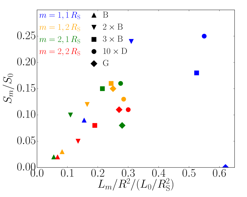
Figure 11: The relation between the relative spiral strength $S_{\rm m}$ and the corresponding integrated torque strength $L_{\rm m}$ for $m=1$ and $m=2$ modes, where $L_{0}=G(10^{10}\mathrm{M_{\odot}})(\mathrm{Gyr})(\mathrm{kpc})^{-1}$ is a unit constant. Here we normalize the integrated torque strength $L_{\rm m}$ by the square of radius, $R^{2}$, to account for the fact that the angular acceleration of particles at different radii is proportional to $R^{-2}$. Different $m$ modes and different radii ($1\,R_{\rm S}$ and $2\,R_{\rm S}$) are shown with different colours, while different symbols stand for different subhaloes, as listed in the legend. There is a good proportional relation between the spiral strength and the time-integrated torque strength across different radii and different $m$ modes, with only a few outliers (see main text for more details).

The underlying reason for the strong relation between the spiral strength and the torque strength is that the time window when the subhalo exerts a strong torque on the disc is very short. Specifically, the time span for a subhalo to generate torque on the disc of more than $2\%$ of the peak value is less than $200\,\mathrm{Myr}$, except for the fly-by subhalo G, whose time span is about $400\,\mathrm{Myr}$. The typical orbiting period of patterns in the stellar disc ranges from $200\,\mathrm{Myr}$ (for $m=1$ modes at $1\,R_{\rm S}$) to $1200\,\mathrm{Myr}$ (for $m=2$ modes at $4\,R_{\rm S}$). This means that for most of the cases patterns evolve for no more than one orbit during the subhalo impact.

Therefore, modes are generated and evolve in the following way: subhaloes impact the disc impulsively, triggering different $m$ modes. Of these, $m=1$ and $m=2$ modes are the strongest because the torque has a strong $m=1$ and $m=2$ component. Between these two kinds of modes, $m=1$ modes are dominant in the disc first partly because they have the shortest winding time, while $m=2$ modes follow and persist longer because of their flat pattern speed curve. Another cause for stronger $m=1$ modes lies in the fact that $m=1$ torques are generally stronger. In fact, we have calculated the strength of $m=1$ and $m=2$ components of the torque on a ring in the stellar disc at a fixed radius when the subhalo is placed at different positions with respect to the ring. For most regions the $m=1$ component is higher in strength. The $m=2$ strength is higher only in a very small region close to the ring.

For the fly-by subhalo, the impacting time is about two times longer than that of the other subhaloes, comparable to or longer than the period of patterns at $1\,R_{\rm S}$. In this particular case, resonance effects become important, leading to a spiral strength that is lower than the expected value.

4 Conclusion

In this paper, we studied the impact of subhaloes on the stellar disc with a series of $N$-body simulations based on the Aquarius simulations (Springel et al., 2008). To clearly pin down the stellar disc response to subhaloes with realistic properties extracted from the cosmological simulations, we first performed cosmological dark matter-only simulation where we have adiabatically introduced analytic stellar disc potential. We have then parameterized the main dark matter halo (both in terms of its density profile and shape and subject to the presence of the stellar disc) with an analytic potential, fixed as a function of time, while we have represented the stellar disc and all subhaloes found in the original Aquarius simulation with “live” particles. We found four massive subhaloes (subhalo A to F) that pass through the disc, two of which (subhalo A and subhalo B) hit the disc twice (labeled as subhaloes C and E). We also found a massive subhalo that does not impact the disc in the innermost regions but flies over it with a very small impact parameter (subhalo G).

In general these subhaloes cause disc heating, rings, warps, disc lopsidedness, a central bar, as well as strong single- and two-armed spiral structures. There is a significant disc heating and warping during the simulation but only at lower redshifts when the massive fly-by subhalo G passes close to the disc. This agrees well with other previous studies (e.g. Velazquez & White, 1999; Kazantzidis et al., 2009; Moetazedian & Just, 2016). Increase of the velocity dispersion leads to an increase in Toomre’s $Q$ parameter, which helps stabilize the disc from self-gravity-induced spiral structures.

Further to disc heating and warping, strong single-armed and two-armed spiral structures develop in the disc. Generally, single-armed spiral structures are apparent first but wind up quickly, and two-armed spiral structures become prominent after single-armed spiral structures wind up. The winding rate of the spiral structures can be well understood by studying the slope of inner Lindblad resonances, as both single-armed and two-armed spirals turn out to be kinematic density waves whose pattern speed follows inner Lindblad resonances. The curve of $\Omega-\kappa/m$ is steeper for $m=1$ then for $m=2$ at all radii, which leads to a faster winding rate of $m=1$ modes. Nevertheless, the winding rate for the outer region of the disc is significantly lower (both for $m=1$ and $m=2$ modes), such that spiral structures can persist for several $\mathrm{Gyrs}$.

In the inner region of the stellar disc, three distinctive generations can be found for the fast-winding single-armed spiral structures, which we attribute to subhalo A, B and G, respectively. We demonstrated such correlation by showing that spiral structures are not present when we remove the corresponding subhaloes, and that the peak strength of spiral structures in most cases correlates very well with the torque exerted by the subhalo. This shows that the majority of interactions between the subhaloes and the disc in our simulations are impulsive with resonances playing a minor role. The fact that strong spiral structures form in response to each massive subhalo, i.e. with a mass comparable to that of the disc, may provide a way to probe the properties of subhaloes interacting with the central galaxy. However, we caution that a further study taking into account the effect of main dark matter halo which is live (rather than static as assumed here) and considering stellar discs with different masses will be needed to shed light on the relation between subhaloes and spiral structures.

It is worth reiterating that we have not simulated the main dark matter halo with live particles to avoid generations of spurious modes in the disc due to the coarse graininess of the halo (i.e. due to the Poisson noise) which is inevitable in present state-of-the-art simulations. In reality, however, subhaloes will suffer from a stronger dynamical friction caused by the main dark matter halo, which may influence the evolution of the subhaloes. We have verified that this does not effect our results in any significant way, as the mass loss of subhaloes is similar regardless of the presence of the live halo as is the time spent in the vicinity of the disc during which subhaloes exert most torque and resonances.

A live dark matter halo may also have an impact on the torque strength and on the waves in the stellar disc. As subhaloes approach the innermost regions, the centre of the dark matter halo and the stellar disc moves slightly in accord with the movement of subhaloes. This may result in a smaller $m=1$ torque (for further details see Appendix D). Additionally, in a live dark matter main halo, subhaloes may lead to distortions in the inner halo, which in turn act upon subhaloes and the disc, and damp bending waves in the disc (Sellwood et al., 1998; Nelson & Tremaine, 1995). As far as the warp structures are concerned, distortions of the inner dark matter main halo due to a passing subhalo can amplify the torques exerted on the disc (Weinberg, 1998; Vesperini & Weinberg, 2000; Gómez et al., 2016). We expect such effects also exist for spiral structures, which may even lead to stronger responses when a live dark matter main halo is present. In this work, we focus only on the impact of torques generated by the subhaloes. A study including the response of the dark matter main halo will require very high resolution simulations (similar to the resolution of level-1 Aquarius simulation), which is beyond the scope of this paper.

Our results demonstrate a clear link between the modes in the disc and the individual passages of massive satellites with realistic masses and orbits extracted from cosmological simulations. Over $7$ Gyrs of cosmic time only $2-3$ encounters are needed to continuously re-generate and sustain grand-design spiral arms in the disc. Our stellar disc has been intentionally setup to have a high Toomre’s $Q$ profile throughout, making it possible to isolate the effects of subhaloes only. With a disc more dominated by self-gravity we expect that grand-design spiral arms triggered by satellites will themselves be a source of flocculent arms thanks to swing amplification. Hence, stellar disc interaction with satellites, within the standard hierarchical structure formation scenario, appears as a very promising and natural way of generating a variety of spiral structures in the discs as well as bars, warps, tilted rings and lopsidedness.

Appendix A Fitting Function for the Halo

In this appendix we describe our fitting function to the density distribution of the smooth part of dark matter halo in the Phase-3 simulation. For the radial density distribution, we split the profile into two regions: the main halo profile $\rho_{\mathrm{I}}(r)$ and the outer region profile $\rho_{\mathrm{O}}(r)$. We fit the main halo region with two Einasto profiles, namely

$$\rho_{\mathrm{I}}(r)=\begin{cases}\rho_{\mathrm{1}}\exp\left[-\frac{2}{\alpha_{1}}\left(\left(r/R_{\mathrm{1}}\right)^{\alpha_{1}}-1\right)\right]&\text{if }r<R_{\mathrm{1}},\\ \rho_{\mathrm{1}}\exp\left[-\frac{2}{\alpha_{2}}\left(\left(r/R_{\mathrm{1}}\right)^{\alpha_{2}}-1\right)\right]&\text{otherwise }\end{cases}$$ (12)

where $R_{\mathrm{1}}=10\,\mathrm{kpc}$ is the scale radius, $\rho_{\mathrm{1}}=9\times 10^{6}\,\mathrm{M_{\odot}}/\mathrm{kpc}^{3}$ is the scale density, $\alpha_{1}=0.2$ and $\alpha_{2}=0.07$ are two shape parameters.

The outer region is fitted with a single Einasto profile,

$$\rho_{\mathrm{O}}=\rho_{\mathrm{2}}\exp\left[-\frac{2}{\alpha_{3}}\left(\left(r/R_{\mathrm{2}}\right)^{\alpha_{3}}-1\right)\right],$$ (13)

where $R_{2}=1.3\,\mathrm{Mpc}$ is the scale radius, $\rho_{2}=1.598\times 10^{2}\,\mathrm{M_{\odot}}/\mathrm{kpc}^{3}$ is the scale density and $\alpha_{3}=3$ is the shape parameter. The spherical density distribution of the whole halo is then

$$\rho_{\mathrm{S}}(r)=\rho_{\mathrm{I}}(r)+\rho_{\mathrm{O}}(r).$$ (14)

The resulting spherically averaged halo profile, compared with the simulated dark matter halo profile is shown in the left panel of Figure 12.

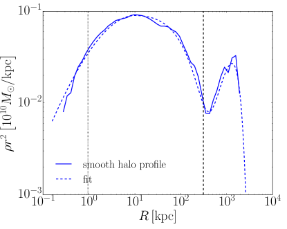
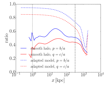
Figure 12: Fit to the smooth part of the halo in a simulation with the Aq-A halo and a static disc potential. The smooth part includes all particles except for those that become part of subhaloes from $z=1$ to $z=0$. In both plots, the solid curves represents the data while the dashed curves represent our analytical model. Left: the $\rho r^{2}$ profile, where $\rho$ is the spherically averaged density. The valley in the density profile at $R=400\,\mathrm{kpc}$ marks the outer boundary of the main halo. Right: the halo shape, i.e. the ratios of the three axes: $p=b/a$ and $q=c/a$, where $a$, $b$ and $c$ are the length of three axes with $a>b>c$. We model the dark matter halo with triaxial models whose central region is more spherical than the data to account for the missing baryonic effect. The vertical dotted lines in both plots indicate $2.8\,\epsilon=0.96\,\mathrm{kpc}$, where $\epsilon$ is the softening length of dark matter particle. The vertical dashed lines represent the virial radius of the halo.

We do not set up the axis ratio profiles of our triaxial dark matter halo model by fitting the triaxial profile of the simulated dark matter halo directly, since we expect a much rounder inner halo profile due to missing baryonic effects. Instead, we model the axis ratios $p=b/a$ and $q=c/a$ with the following equation

$$p(r)=0.35+\frac{0.6}{1+\exp\left[\log(r/r_{\rm c})/\log(r_{\rm s})\right]}\,,$$ (15)

and

$$q(r)=0.25+\frac{0.6}{1+\exp\left[\log(r/r_{\rm c})/\log(r_{\rm s})\right]}\,,$$ (16)

where $r_{\rm c}=5.01\times 10^{2}\,\mathrm{kpc}$ and $r_{\rm s}=3.16\,\mathrm{kpc}$ are the two shape parameters. The triaxial profile is implemented in the simulation as two spherical harmonic density components as described in Appendix B.

Appendix B Estimating Triaxial Density Profile

We need to relate the triaxial profile of the halo with the density profiles representing two triaxial parts $\rho_{\mathrm{T1}}(r)$ and $\rho_{\mathrm{T2}}(r)$ before we can use it in the simulation. The density distribution on the three axes is related to $\rho_{\mathrm{T1}}$ and $\rho_{\mathrm{T2}}$ through

$$\rho_{\mathrm{x}}(r)= \rho_{\mathrm{S}}(r)+\frac{1}{2}\rho_{\mathrm{T1}}(r)+3\rho_{\mathrm{T2}}(r),$$ (17)

$$\rho_{\mathrm{y}}(r)= \rho_{\mathrm{S}}(r)+\frac{1}{2}\rho_{\mathrm{T1}}(r)-3\rho_{\mathrm{T2}}(r),$$ (18)

$$\rho_{\mathrm{z}}(r)= \rho_{\mathrm{S}}(r)-\rho_{\mathrm{T1}}(r).$$ (19)

We have to find $\rho_{\mathrm{T1}}(r)$ and $\rho_{\mathrm{T2}}(r)$ so that the triaxial profile is satisfied, i.e.

$$\rho_{\mathrm{x}}(r)=\rho_{\mathrm{y}}(rp(r))=\rho_{\mathrm{z}}(rq(r)).$$ (20)

This equation is hard to solve analytically. We therefore approximate it by assuming that locally the density profile follows a power law of index $\frac{\mathrm{d}\log(\rho)}{\mathrm{d\log(r)}}$. We can rewrite Equation (20) as

$$\rho_{\mathrm{x}}(r)=\frac{\rho_{\mathrm{y}}(r)}{p(r)^{\alpha}}=\frac{\rho_{\mathrm{z}}(r)}{q(r)^{\alpha}},$$ (21)

where $\alpha=-\frac{\mathrm{d}\log(\rho)}{\mathrm{d\log(r)}}$ is the negative power law index. Solving this equation yields Equation (2) and (3). We implement this approximation and calculated the resulting triaxial profile, as shown in the right panel of Figure 12. The profile is rounder in the inner region and gradually decreases to the simulated profile at the outer region, as expected.

Appendix C Calculating Halo Potential from Its Density Profile

The density distribution of our smooth halo follows Equation (4). It is trivial to calculate the potential for the spherical component $\rho_{\mathrm{S}}(r)$. To calculate potential of the triaxial part, we start from the Poisson’s equation

$$\nabla^{2}\Phi_{\mathrm{T}}(r,\theta,\phi)=4\pi G\rho_{\mathrm{T}}(r,\theta,\phi)\,.$$ (22)

Assuming

$$\Phi_{\mathrm{T}}(r,\theta,\phi)=\sum_{m}\sum_{l}\Phi_{\mathrm{T},m}^{l}(r)Y_{m}^{l}(\theta,\phi)\,,$$ (23)

and taking the density form as

$$\rho_{\mathrm{T}}(r,\theta,\phi)=\rho_{\mathrm{T}}(r)Y_{2}^{l_{0}}(\theta,\phi)\,,$$ (24)

where $l_{0}$ can be $0$ and $2$ for the two spherical harmonic functions used in our model. We can easily find that $\Phi_{\mathrm{T},m}^{l}(r)$ is non-zero if and only if $m=2$ and $l=l_{0}$. For simplicity we let $\Phi_{\mathrm{T}}(r)=\Phi_{\mathrm{T},2}^{l_{0}}(r)$. We find

$$\frac{1}{r^{2}}\frac{\partial}{\partial r}\left(r^{2}\frac{\partial}{\partial r}\Phi_{\mathrm{T}}(r)\right)-\frac{6}{r^{2}}\Phi_{\mathrm{T}}(r)=4\pi G\rho_{\mathrm{T}}(r)\,.$$ (25)

The second term on LHS is contributed by $\nabla^{2}Y_{2}^{l}(\theta,\phi)$. Green’s function for a delta density function at $r_{0}$, i.e. $\rho_{\mathrm{T}}(r)=\delta(r-r_{0})$, is

$$\mathcal{G}(r,r_{0})=-\frac{1}{5}\frac{r_{<}^{2}}{r_{>}^{3}}\,,$$ (26)

where $r_{<}$ and $r_{>}$ is the smaller and larger value in $r$ and $r_{0}$, respectively. The solution to the equation is hence

$$\Phi_{\mathrm{T}}(r)=4\pi G\int_{0}^{\infty}\mathcal{G}(r,r_{0})\rho_{\mathrm{T}}(r_{0})r_{0}^{2}\,\mathrm{d}r_{0}\,.$$ (27)

where we convolve the density profile $\rho_{\mathrm{T}}(r_{0})$ over the radius $r_{0}$ from 0 to $\infty$ with Green’s function $\mathcal{G}(r,r_{0})$. The potential and the force of the halo can then be calculated accurately with a 1-dimensional integration in the simulation.

Appendix D The Artificial Torque caused by the Fixed Dark Matter Main Halo

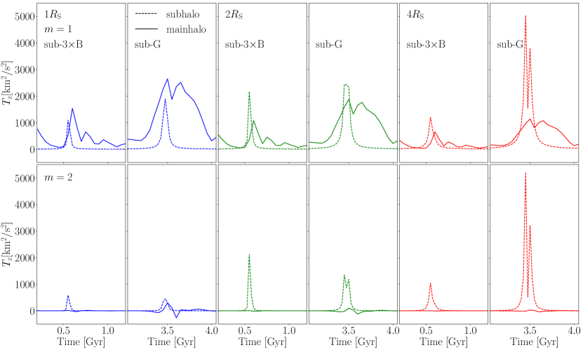
Figure 13: Comparison of torques generated by the displaced main halo and subhaloes $3\times$B and G. The torques at $1R_{\mathrm{S}}$, $2R_{\mathrm{S}}$ and $4R_{\mathrm{S}}$ of $m=1$ (top panels) and $m=2$ (bottom panels) are shown. The torque generated by the main halo is shown with solid curves while the torque from subhaloes is shown with dashed curves. For $m=1$ modes at $1R_{\mathrm{S}}$, the artificial torque from the displaced main halo is comparable to the torque from the subhaloes, while in the outer regions it becomes smaller. The torque from the main halo is negligible for $m=2$ modes.

As a subhalo approaches the innermost region of the system, the centre of both the stellar disc and the dark matter main halo may noticeably move in response to the gravitational force from the subhalo. In our simulation, however, the main dark matter halo is included as a fixed potential, and only the stellar disc responds to the approaching subhalo. This leads to a displacement between the main halo and the disc and hence an artificial torque from the main dark matter halo.

In this appendix we estimate the upper limit on such a torque. We first calculate the displacement of the disc from its original location. We find that for most of the time, the disc moves no further than $0.3\mathrm{kpc}$ ($\sim 0.1R_{\mathrm{S}}$) from its original location, with the only exception of a displacement of $0.82\mathrm{kpc}$ ($\sim 0.26R_{\mathrm{S}}$) when the subhalo G flies over the disc. Note that in reality only the inner region of the dark matter main halo should move in a similar way to that of the disc centre. Therefore in our simulation, the artificial torque results mostly from the fixed inner region of the main halo. Nevertheless, for a rough estimate of the upper bound on such an effect, we consider the main halo as a whole and calculate the torque due to its displacement with respect to the disc using equation (10).

The comparison of this torque, which is highest in the case of the passage of subhalo G, and that caused by subhalo G itself is shown in Figure 13. We also show the results for subhalo B with three times its original mass for comparison. Due to the triaxiality of the main halo, there is a non-zero $m=2$ torque even when the disc is not displaced. For a better comparison, we plot the difference from that non-zero initial torque instead of the absolute value for $m=2$ torques.

For $m=2$ modes, the torque from the main halo is generally much smaller compared to that from subhaloes $3\times$B and G, except at $1R_{\mathrm{S}}$ where torques from both are weak. Therefore our results on $m=2$ spiral structures should be in general unaffected by the artificial torque from the fixed halo. For $m=1$ modes at $4R_{\mathrm{S}}$ the contribution from the displaced halo is weak as well, but it grows in significance moving inwards, and at $1R_{\mathrm{S}}$ it is comparable to the torque caused by subhaloes $3\times$B and G. Note however as mentioned before, the torque calculated here is likely the upper bound both in terms of the peak value and the non-zero torque width.

We further find that the phase of the torque from the displaced main halo follows closely that from subhaloes, therefore enhancing the $m=1$ spiral structures in our simulations. In a simulation with a live main halo, it is hence possible that the $m=1$ torque from the main halo may be weaker or even offset a portion of the torque from subhaloes, therefore leading to weaker $m=1$ spiral structures. Calculating this effect precisely requires dedicated, very high resolution simulations with a live dark matter halo and is beyond the scope of this work.

Appendix E Removing subhalo A and B

Further to Section 3.5 where we study the impact of each halo, we also run a simulation with subhalo A and B removed at a same time. Note that since subhaloes A and C are the same subhalo hitting the disc twice, in this simulation subhalo C is also removed. As shown in Figure 14, when subhaloes A and B are both removed, only very weak modes develop for $z>0.7$, demonstrating that the first two generation of modes are mainly caused by subhaloes A and B.

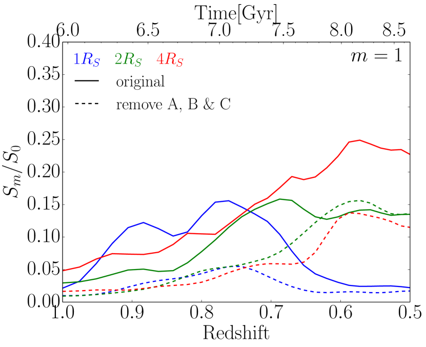
Figure 14: Simulation with subhaloes A and B removed. The first and the second generation of modes are absent, demonstrating clearly that these modes are mostly caused by subhaloes A and B.

Appendix F Subhalo inspirals in live and static haloes

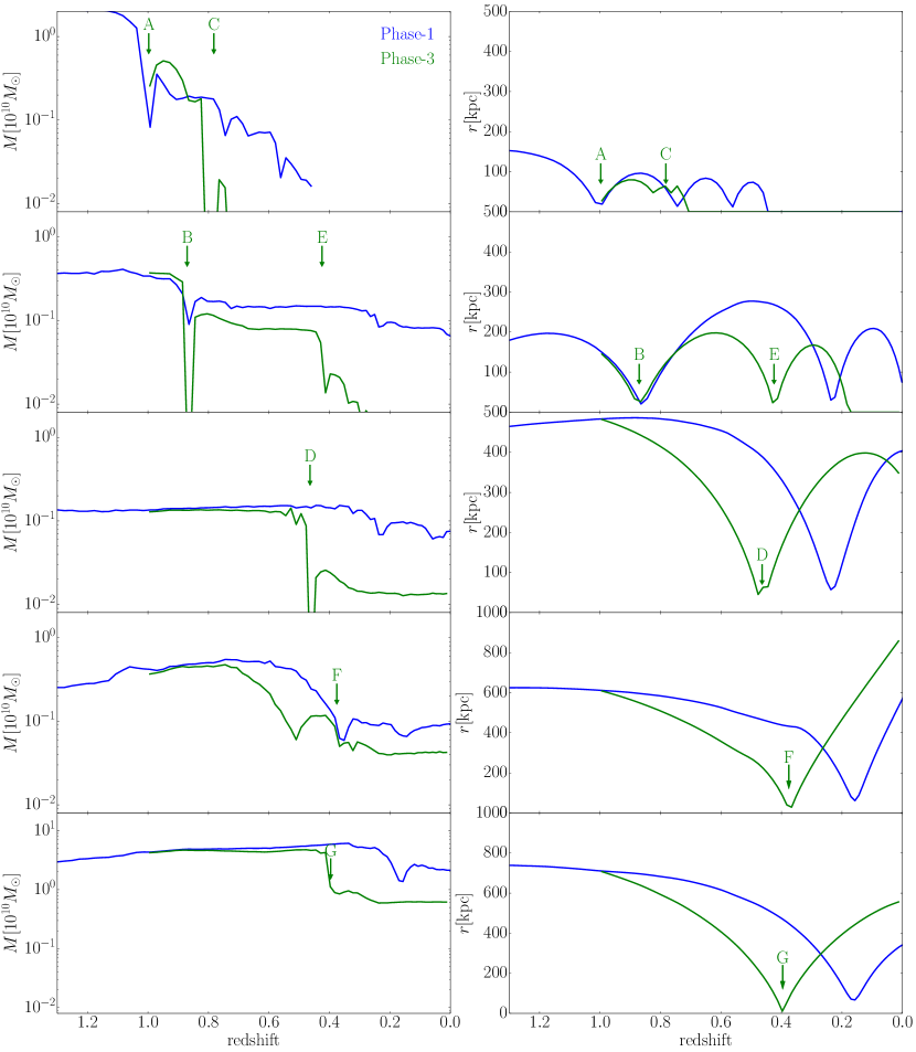
Figure 15: Mass evolution (left) and distance from the centre (right) of subhaloes as they pass through the central region of the halo and the disc. The impact times in the Phase-3 simulation of the subhaloes are marked with vertical arrows. Up to the passage through the pericentre mass loss is comparable in the two simulations. For earlier impacts (subhaloes A, B and C), the impacting time corresponds very well between the two simulations, while impacts happen earlier in the Phase-3 simulation for subhaloes D to G. Note that subhaloes A/C and B/E are largely disrupted at the later times of the simulation, where we truncate the curves.

To study the influence of substituting the live main dark matter halo with an analytic halo potential, we compare the inspiral of subhaloes listed in Table 1 in the Phase-1 and Phase-3 simulation. The evolution of each subhalo’s mass and distance from the centre of the main halo is illustrated in Figure 15. As shown in left panels, subhaloes lose significant amount of mass every time they go through the central region of the main halo. The mass loss with a live halo (in blue) and with an analytic halo (in green) is generally comparable up to the pericentric passage, ranging from $50\%$ to $80\%$. However, after the passage trough the stellar disc the mass loss of subhaloes is typically larger in the Phase-3 than in the Phase-1 simulation (which does not contain a live stellar disc).

As can be seen from the panels on the right, for subhaloes A, B and C the time of the pericentric passage in the two simulations is very similar (as majority of their trajectory has been computed prior to the start of the Phase-3 with the live dark matter halo present), while other subhaloes reach pericentre somewhat earlier in the Phase-3 than in the Phase-1 simulation. This is due to the fact that in the Phase-3 simulation, the lack of the main dark matter halo leads to a much lower dynamical friction on the subhaloes. Nonetheless, this should not affect our results regarding the response of the stellar disc to the subhaloes. In fact, we have verified that the velocity of the impact is comparable (within a factor of $1.2$) and that the time subhaloes spend within half of the apocentre is comparable as well (within factors of $0.85$ to $1.17$).

References

- Athanassoula (1978) Athanassoula E., 1978, A&A, 69, 395
- Bose et al. (2017) Bose S., Hellwing W. A., Frenk C. S., Jenkins A., Lovell M. R., Helly J. C., Li B., Gonzalez-Perez V., Gao L., 2017, MNRAS, 464, 4520
- Bowden et al. (2013) Bowden A., Evans N., Belokurov V., 2013, Monthly Notices of the Royal Astronomical Society, 435, 928
- Boylan-Kolchin et al. (2008) Boylan-Kolchin M., Ma C.-P., Quataert E., 2008, MNRAS, 383, 93
- Bullock (2010) Bullock J. S., 2010, ArXiv e-prints
- Collins et al. (2010) Collins M. L. M., Chapman S. C., Irwin M. J., Martin N. F., Ibata R. A., Zucker D. B., Blain A., Ferguson A. M. N., Lewis G. F., McConnachie A. W., Peñarrubia J., 2010, MNRAS, 407, 2411
- DeBuhr et al. (2012) DeBuhr J., Ma C.-P., White S. D., 2012, Monthly Notices of the Royal Astronomical Society, 426, 983
- Dekel & Silk (1986) Dekel A., Silk J., 1986, ApJ, 303, 39
- Diemand & Moore (2011) Diemand J., Moore B., 2011, Advanced Science Letters, 4, 297
- Dolag et al. (2009) Dolag K., Borgani S., Murante G., Springel V., 2009, MNRAS, 399, 497
- D’Onghia et al. (2010) D’Onghia E., Springel V., Hernquist L., Keres D., 2010, ApJ, 709, 1138
- D’Onghia et al. (2013) D’Onghia E., Vogelsberger M., Hernquist L., 2013, The Astrophysical Journal, 766, 34
- Dubinski & Chakrabarty (2009) Dubinski J., Chakrabarty D., 2009, The Astrophysical Journal, 703, 2068
- Dubinski et al. (2008) Dubinski J., Gauthier J.-R., Widrow L., Nickerson S., 2008, in Funes J. G., Corsini E. M., eds, Formation and Evolution of Galaxy Disks Vol. 396 of Astronomical Society of the Pacific Conference Series, Spiral and Bar Instabilities Provoked by Dark Matter Satellites. p. 321
- Efstathiou (1992) Efstathiou G., 1992, MNRAS, 256, 43P
- Erkal & Belokurov (2015) Erkal D., Belokurov V., 2015, MNRAS, 454, 3542
- Fouvry et al. (2015) Fouvry J. B., Pichon C., Magorrian J., Chavanis P. H., 2015, A&A, 584, A129
- Gao et al. (2004) Gao L., White S. D. M., Jenkins A., Stoehr F., Springel V., 2004, MNRAS, 355, 819
- Gómez et al. (2012) Gómez F. A., Minchev I., Villalobos Á., O’Shea B. W., Williams M. E. K., 2012, MNRAS, 419, 2163
- Gómez et al. (2017) Gómez F. A., White S. D. M., Grand R. J. J., Marinacci F., Springel V., Pakmor R., 2017, MNRAS, 465, 3446
- Gómez et al. (2016) Gómez F. A., White S. D. M., Marinacci F., Slater C. T., Grand R. J. J., Springel V., Pakmor R., 2016, MNRAS, 456, 2779
- Grand et al. (2016) Grand R. J. J., Springel V., Gómez F. A., Marinacci F., Pakmor R., Campbell D. J. R., Jenkins A., 2016, MNRAS, 459, 199
- Howard et al. (1993) Howard S., Keel W. C., Byrd G., Burkey J., 1993, ApJ, 417, 502
- Hu & Sijacki (2016) Hu S., Sijacki D., 2016, MNRAS, 461, 2789
- Jiang et al. (2008) Jiang C. Y., Jing Y. P., Faltenbacher A., Lin W. P., Li C., 2008, ApJ, 675, 1095
- Kazantzidis et al. (2009) Kazantzidis S., Zentner A. R., Kravtsov A. V., Bullock J. S., Debattista V. P., 2009, ApJ, 700, 1896
- Klypin et al. (1999) Klypin A., Kravtsov A. V., Valenzuela O., Prada F., 1999, ApJ, 522, 82
- Koposov et al. (2015) Koposov S. E., Belokurov V., Torrealba G., Evans N. W., 2015, ApJ, 805, 130
- Larson (1974) Larson R. B., 1974, MNRAS, 169, 229
- Lindblad (1963) Lindblad B., 1963, Stockholms Observatoriums Annaler, 22, 5
- Lovell et al. (2014) Lovell M. R., Frenk C. S., Eke V. R., Jenkins A., Gao L., Theuns T., 2014, MNRAS, 439, 300
- Lynds & Toomre (1976) Lynds R., Toomre A., 1976, ApJ, 209, 382
- Mateo (1998) Mateo M. L., 1998, ARA&A, 36, 435
- McConnachie et al. (2009) McConnachie A. W., Irwin M. J., Ibata R. A., Dubinski J., Widrow L. M., e.a. 2009, Nature, 461, 66
- Minchev et al. (2009) Minchev I., Quillen A. C., Williams M., Freeman K. C., Nordhaus J., Siebert A., Bienaymé O., 2009, MNRAS, 396, L56
- Moetazedian & Just (2016) Moetazedian R., Just A., 2016, MNRAS, 459, 2905
- Moore et al. (1999) Moore B., Ghigna S., Governato F., Lake G., Quinn T., Stadel J., Tozzi P., 1999, ApJ, 524, L19
- Navarro et al. (1996) Navarro J. F., Eke V. R., Frenk C. S., 1996, MNRAS, 283, L72
- Nelson & Tremaine (1995) Nelson R. W., Tremaine S., 1995, MNRAS, 275, 897
- Peñarrubia et al. (2010) Peñarrubia J., Benson A. J., Walker M. G., Gilmore G., McConnachie A. W., Mayer L., 2010, MNRAS, 406, 1290
- Pettitt et al. (2016) Pettitt A. R., Tasker E. J., Wadsley J. W., 2016, MNRAS, 458, 3990
- Purcell et al. (2011) Purcell C. W., Bullock J. S., Tollerud E. J., Rocha M., Chakrabarti S., 2011, Nature, 477, 301
- Quillen et al. (2009) Quillen A. C., Minchev I., Bland-Hawthorn J., Haywood M., 2009, MNRAS, 397, 1599
- Sawala et al. (2016) Sawala T., Frenk C. S., Fattahi A., Navarro J. F., Bower R. G., Crain R. A., Dalla Vecchia C., Furlong M., Helly J. C., Jenkins A., Oman K. A., Schaller M., Schaye J., Theuns T., Trayford J., White S. D. M., 2016, MNRAS, 457, 1931
- Sellwood (2012) Sellwood J. A., 2012, ApJ, 751, 44
- Sellwood & Carlberg (2014) Sellwood J. A., Carlberg R. G., 2014, ApJ, 785, 137
- Sellwood et al. (1998) Sellwood J. A., Nelson R. W., Tremaine S., 1998, ApJ, 506, 590
- Springel (2005) Springel V., 2005, Monthly Notices of the Royal Astronomical Society, 364, 1105
- Springel et al. (2005) Springel V., Di Matteo T., Hernquist L., 2005, Monthly Notices of the Royal Astronomical Society, 361, 776
- Springel et al. (2008) Springel V., Wang J., Vogelsberger M., Ludlow A., Jenkins A., Helmi A., Navarro J. F., Frenk C. S., White S. D. M., 2008, MNRAS, 391, 1685
- Springel et al. (2001) Springel V., White S. D. M., Tormen G., Kauffmann G., 2001, MNRAS, 328, 726
- Taylor & Babul (2004) Taylor J. E., Babul A., 2004, MNRAS, 348, 811
- Thomasson et al. (1989) Thomasson M., Donner K. J., Sundelius B., Byrd G. G., Huang T.-Y., Valtonen M. J., 1989, A&A, 211, 25
- Tollerud et al. (2008) Tollerud E. J., Bullock J. S., Strigari L. E., Willman B., 2008, ApJ, 688, 277
- Toomre & Toomre (1972) Toomre A., Toomre J., 1972, ApJ, 178, 623
- Velazquez & White (1999) Velazquez H., White S. D. M., 1999, MNRAS, 304, 254
- Vera-Ciro et al. (2011) Vera-Ciro C. A., Sales L. V., Helmi A., Frenk C. S., Navarro J. F., Springel V., Vogelsberger M., White S. D. M., 2011, MNRAS, 416, 1377
- Vesperini & Weinberg (2000) Vesperini E., Weinberg M. D., 2000, ApJ, 534, 598
- Weinberg (1998) Weinberg M. D., 1998, MNRAS, 299, 499