Efficient Legendre polynomials transforms:
from recurrence relations to Schoenberg’s theorem

Abstract.

We report results on various techniques which allow to compute the expansion into Legendre (or in general Gegenbauer) polynomials in an efficient way. We describe in some detail the algebraic/symbolic approach already presented in Ref.[1] and expand on an alternative approach based on a theorem of Schoenberg [2].

1. Introduction

This investigation stems from a problem regarding unitarity of the pion-pion scattering amplitude in a model proposed by Veneziano and Yankielowicz: one is given the function

(1) $$A(x,M,\alpha)\equiv\sum_{k\in\rm{div}{(M\!+\!1)}}\,c_{k}(\beta,\gamma)\,\frac{1-\alpha\!+\!M+t}{q_{k}!}\;\frac{\Gamma(q_{k}+(\alpha+t)/k)}{\Gamma((\alpha+t)/k)}$$

where the sum runs over the divisors of $M\!\!+\!\!1$, $t=\tfrac{1}{2}(x-1)(1-\alpha+M)$, $x=\cos\vartheta$ ($\vartheta$ is the scattering angle), $\alpha\in(0,1)$ is the Regge slope, $q_{k}=(M+1)/k-1$ and $M=s+\alpha-1$ is a non–negative integer. The coefficients $c_{k}$ are assumed to be given by $c_{k}\propto k^{-(1+\beta)}\,(1+(\log k)^{-\gamma})$, $\beta$ is a real positive parameter ($\beta=2$ is the most popular value) and usually one assumes $\gamma=\beta\!+\!1$. The problem is to determine the range of the real parameters $(\alpha,\beta,\gamma)$ for which the coefficients of the expansion

$${\mathcal{A}}(s,t)\equiv A(x,M,\alpha)=\sum_{n\geq 0}a_{n}\,P_{n}(x)$$

into Legendre polynomials are all non–negative.

At first sight the problem looks rather trivial; one has only to compute the coefficients by Legendre–Fourier inversion

(2) $$a_{n}\propto\int_{-1}^{1}\,{\mathrm{d}}{x}\;A(x,M,\alpha)\,P_{n}(x)\;.$$

and check their sign. However, in practice, one has to face a variety of problems. The number of integrals to be computed is very high if one wants to explore the “critical landscape” parametrized by the pairs $(\beta,M)$ and identify the critical value $\alpha_{\rm crit}=\sup_{M}\alpha(\beta,M)$ such that positivity occurs for $\alpha>\alpha_{\rm crit}$ and for all $M$. Moreover the function to be analyzed is a high–degree polynomial which makes the integrals rather sensitive to accuracy. Hence it is advisable to employ exact arithmetic or at least extended precision. This is easily achieved using a symbolic language like Mathematica or adopting an extended precision package in Matlab. We found that an alternative technique, not requiring the calculation of even a single integral, is however preferable if one wants to reach the result in a reasonable time. Another strategy, which also does not require to compute Fourier coefficients explicitly, has been developed based on a theorem of Schoenberg which relates the non–negativity of the expansion coefficients to a positivity property of some matrices built out of the function $A(s,t)$. In the following sections we present the “algebraic approach” and the “Schoenberg’s theorem” approach.

2. The algebraic approach

We note that $A(x,M,\alpha)$ is a polynomial of degree $M\!+\!1$ which is defined as a sum of terms which are easily factorized in simple monomials, being a quotient of gamma-functions (Pochammer’s symbols). It follows that an easy technique to derive its expansion into Legendre polynomials is provided by the recurrence relation

(3) $$x\,P_{n}(x)=\frac{n\!+\!1}{2n\!+\!1}\,P_{n+1}(x)+\frac{n}{2n\!+\!1}\,P_{n-1}(x)\;.$$

On the $d-$dimensional sphere $S^{d}$ one has to consider the recurrence for Gegenbauer’s polynomials, namely

(4) $$x\,C^{\lambda}_{n}(x)=\frac{n\!+\!1}{2(n\!+\lambda)}\,C^{\lambda}_{n\!+\!1}(x)\!+\!\frac{n\!+2\lambda-1}{2(n\!+\lambda)}\,C^{\lambda}_{n-1}(x),\;\left(\lambda=\tfrac{1}{2}(d-1)\right)\;.$$

Let $A_{k}=\prod_{j}(x-x_{j})$ be the factorization of the $k-th$ term in Eq.(1), suitably normalized; starting from $A_{k,0}(x)\equiv 1$ and applying the first factor we get

$$A_{k,1}=(x-x_{1})=P_{1}-x_{1}\,P_{0}$$

and, subsequently

$$A_{k,2} =(x-x_{2})\,A_{k,1}=x(P_{1}-x_{1}\,P_{0})-x_{2}(P_{1}-x_{1}\,P_{0})$$

$$=\frac{2}{3}P_{2}-(x_{1}+x_{2})P_{1}+(x_{1}x_{2}+\frac{1}{3})P_{0}$$

and so forth, so that after applying this formula a number of times to reach the degree of the polynomial, we get by inspection the required expansion. The process is easily realized by using a symbolic language like Mathematica or form; alternatively we can represent the multiplication by a factor $x$ as an infinite matrix

$${\mathcal{X}}=\begin{pmatrix}0&\frac{1}{3}&0&0&0&0&\ldots\\ 1&0&\frac{2}{5}&0&0&0&\ldots\\ 0&\frac{2}{3}&0&\frac{3}{7}&0&0&\ldots\\ 0&0&\frac{3}{5}&0&\frac{4}{9}&0&\ldots\\ \vdots&&&\ddots&&\ddots&\end{pmatrix}$$

and in general for any dimension, using Eq. (4). The expansion is then computed by applying the product $\prod_{j}({\mathcal{X}}-x_{j})$ to the initial vector $A_{k,0}=\{1,0,0,\ldots\}^{\prime}$. Let us note that using a symbolic approach makes it possible to derive the result by working with symbolic parameters $(a,\beta)$ ; using a floating point representation for the coefficients, instead, one loses this possibility and moreover one has to pay attention to arithmetic accuracy, since floating point errors can be amplified in the process. Hence in a floating point approach one has to use multiple precision arithmetic. Having developed an efficient algorithm to compute the expansion coefficients, the range of values in the $(\alpha,\beta)$ plane where positivity holds for any $M$ can be determined by the classical bisection method in the following way:

1. fix a value for $M$ and $\beta$;

2. fix a tolerance $\varepsilon$, e.g. $\varepsilon=10^{-6}$;

3. start with an interval for $\alpha$, say $\alpha_{\rm min}=0$, $\alpha_{\rm max}=1$ such that positivity is known to hold for $\alpha=1$ and it does not hold for $\alpha=0$;

4. compute the coefficients at the midpoint $\alpha=\tfrac{1}{2}(\alpha_{\rm min}+\alpha_{\rm max})$;

5. if all coefficients are positive, then set $\alpha_{\rm max}=\alpha$, otherwise set $\alpha_{\rm min}=\alpha$;

6. repeat until $|\alpha_{\rm max}-\alpha_{\rm min}|\leq\varepsilon$ and keep the mean value as $\alpha_{\rm crit}(M,\beta)$ up to $O(\varepsilon)$;

7. loop on $M$ and $\beta$ .

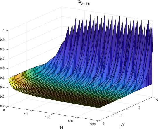
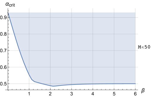
One is interested to identify the points $(\alpha,\beta)$ where positivity holds for every $M$, i.e. we have to compute $\alpha_{\rm crit}(\beta)=\max_{M}\alpha_{\rm crit}(M,\beta)$. This requires, of course, a compromise, since we have to fix a maximum value of $M$ to make the calculation in a finite time, but a posteriori we see that after some large $M\approx 100$ the profile stabilizes. Here we borrow some pictures from Ref[1] (Fig.1 and 2).

Figure 1. The “critical landscape”: values of $\alpha$ above the surface give positive residues (here and in the following $\gamma=\beta+1$)

Figure 2. Same as the plot of Fig.1 projected on the ${\footnotesize(\beta,\alpha)}$ plane. Shaded region corresponds to positive residues.

2.1. Chebfun

A very simple approach, which essentially makes it trivial to write the floating point code, adopts the Chebfun environment in Matlab. Here the expansion coefficients are built in and we get the result with essentially a single instruction. The bisection strategy then is again used to get the critical values of $\alpha$. This option, however, would require a multiprecision extension of Chebfun, which is not available at present, and it does not appear to be around the corner. Hence this method has been mainly used for debugging purposes.

2.2. Spectral method

The matrix representing multiplication by $x$, namely $\mathcal{X}$ defined in Eq.(2), is known to have the zeros of the Legendre polynomial $P_{N+1}(x)$ as eigenvalues and its eigenvectors are exactly known in terms of Legendre polynomials of lower indices evaluated at the eigenvalues. This means that we exactly know the spectral representation of ${\mathcal{X}}$ and any function of it can be computed in algebraic form. This is particularly useful if the function to be expanded is not a polynomial. However in this case the maximum order $N$ is not defined, hence it must be introduced as a cutoff, which involves an error in the calculation of the coefficients which must be estimated by extrapolating to large $N$. It turns out that this spectral strategy coincides step by step with the idea of computing the integrals in Eq.(2) by Gaussian quadrature: since this is builtin in Mathematica it does not cost much to try this alternative strategy. Our experience is that we are not going to earn much in terms of computing efficiency. See Ref.[1] for details.

3. The alternative route: Schoenberg’s theorem

The main new contribution of this report regards a further strategy we may adopt to solve the original problem. This is based on a theorem going back to 1942 due to I. J. Schoenberg [2]: given a function $f(\cos\vartheta)$, the positivity of the coefficients in its expansion into Legendre functions is directly linked to a property of the function which is know as “positive definiteness” (or “semi-positive definitness”).

Definition: a function $f(\cos\vartheta)$ is said to be positive semi-definite on $S^{d}$ if for any integer $n>0$ and any $n$-tuple of unit vectors $\{\boldsymbol{v}_{1},\ldots,\boldsymbol{v}_{n}\}$ on $S^{d}$ the matrix $F_{ij}\equiv f(\boldsymbol{v_{i}}\cdot\boldsymbol{v}_{j})$ is positive semi-definite, i.e. $\sum_{ij}F_{ij}\,\alpha_{i}\,\alpha_{j}\geq 0$.
Theorem (Schoenberg 1942): A function $f(\cos\vartheta)$ is positive semi-definite if and only if its expansion into Legendre functions has non-negative coefficients.

By “Legendre functions” it is understood Legendre polynomials $P_{\ell}(x)$ in dimension $d=2$, and Gegenbauer’s polynomials $C_{n}^{\lambda}$ in any dimension $d$, with $\lambda=\tfrac{1}{2}(d-1)$.

The question then arises whether this equivalence can be exploited in a practical way to prove positivity of the expansion coefficients. There is an obvious difficulty: the theorem requires in principle to test the positivity of the matrix $F_{ij}$ for every integer $n$ and this is clearly impossible in practice. One is then led to ask whether it would be sufficient to perform the test in a suitable range of values for $n$, say $n<N_{\rm max}$. Assuming that a negative coefficient is present at some level $\ell$, is there a connection between $\ell$ and the range of $n$ which will allow to detect the presence of this negative coefficient? We need some condition similar to what is known to hold in the theory of signals, where getting information about the spectrum of a signal around a frequency $\nu$ requires sampling the signal at least with a frequency $2\nu$ (Nyquist-Shannon theorem). In the case of functions defined on the $d$-dimensional sphere what should be the minimal dimension of the $n$-tuples of vectors which can detect a negative component in the Legendre expansion? To investigate this problem we performed a series of tests which point to a preliminary result: “if the first negative component is at level $\ell$ then one should check positivity with $n$-tuples such that $n$ is at least twice as large as the number of spherical harmonics of index less or equal to $\ell$”. In dimension $2$ this requires testing positivity of the matrix $F$ for $n$-tuples with $n\geq 2(\ell+1)^{2}$, in higher dimensions the correct formula can be found in Ref.[4] or in the book by Hochstadt Ref.[5] (see next section).

In a recent paper by Beatson, W. zu Castell and Xu [6] it is conjectured that a necessary and suffcient condition for positivity for every dimension is that the power expansion $f(x)=\sum c_{k}\,(\cos\vartheta)^{k}$ has all positive Taylor coefficients. Unfortunately again we cannot take profit of this conjecture, since the positivity condition for every $S^{d}$ (any $d$!) which is too strong a requirement to be applied to the amplitude given in Eq.(1) and one readily realizes that the condition is not respected for any value of $\alpha$ signaling the fact that the amplitude fails positivity for sufficiently high dimension (perhaps 25?).

Let us remark that the analysis in terms of Schoenberg’s theorem allows one to infer that, since the set of $n$-tuples in $d$ dimensions contains all $n$-tuples in less than $d$ dimensions, positivity at a given value of the parameters for a given function $f(x)$ in dimension $d$ implies positivity for the same function for all dimensions lower than $d$ . This property has been checked by the algebraic method but is far from obvious looking at the recursion relations. On the other hand this property may be difficult to check numerically, the problem being that going up with $d$ the detection of a negative component requires to go to higher dimensional $n$tuples, typically $n\propto\ell_{0}^{d}$. This means that our estimate of a critical $\alpha_{c}$ in $d-$dimensions can be affected by a systematic error much higher than in lower dimensions. On the other hand, if we choose the same function $f(x)$ and apply the test in various dimensions, we check that positivity in dimension $d_{>}$ implies positivity in dimension $d$ with $d<d_{>}$. From this point of view, let’s say that from an algorithmic point of view, the statement/conjecture of Ref. [6] is rather trivial: in the limit of large dimension it is well-known that $\lim_{d\to\infty}C_{n}^{(d-1)/2}(z)/d^{n}=z^{n}/n!\;,$ hence the series of hyperspherical polynomials converges to a simple Taylor series (see [8], pag.303)!

3.1. Numerical results

The numerical test we have devised runs as follows (initially for dimension 2)

1. build the function $f(x)$ directly as a finite sum of Legendre functions with known coefficients $c_{\ell}$ depending on a parameter $\alpha$, explicitly $c_{\ell}\propto 1-\alpha/\alpha_{0}$ starting at some index $\ell_{\rm min}$;

2. extract an $n$-tuple of unit vectors, $\{\boldsymbol{v}_{1},\ldots,\boldsymbol{v}_{n}\}$ uniformly at random on $S^{d}$;

3. evaluate the spectrum of the matrix $f(\boldsymbol{v}_{i}\cdot\boldsymbol{v}_{j})$;

4. determine the value of $\alpha_{0}$ by a bisection strategy as discussed previously depending on the presence of negative eigenvalues;

5. for each value of $\ell_{\rm min}$ perform the test on a range $n\in\{1,2\,(\ell_{\rm min}\!+\!1)^{2}\}$ and check the accuracy in determining $\alpha_{0}$;

6. repeat (b) a number of times and gather the statistics;

7. examine the dependence of the estimate for $\alpha_{0}$ depending on $n\;.$

8. Extend the experiment to higher dimensions.

3.1.1. Test runs

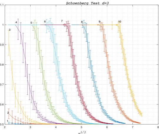
Here we report on a number of test runs in dimension 2, 3, and higher. In the first three runs we examine the effect of applying Schoenberg’s test to functions characterised by the same coefficients in the expansion of hyperspherical polynomials irrespective of dimension. We stress that in this case the coefficients are the same but the functions are different. The critical value for $\alpha$ is the same. The pattern which emerges is the following: for small sets of unit vectors (small $n$) the negative coefficients are often overlooked and as a result the critical $\alpha_{0}$ is overestimated; as $n$ grows the estimate is better and better. If the occurrence of negative components starts at $\ell$ the value of $n$ must be compared to $\ell^{d}$; a rationale for this is probably that the number $H(\ell,d)$ of (hyper)spherical harmonics of index up to $\ell$ on $S^{d}$ grows as $O(\ell^{d})$, precisely

$$H(\ell,2) =(\ell+1)^{2}$$

$$H(\ell,3) =(\ell+1)(2+\ell)(2\ell+3)/6$$

$$H(\ell,4) =(\ell+1)(\ell+2)^{2}(\ell+3)/12$$

$$H(\ell,5) =(1+\ell])(2+\ell)(3+\ell)(4+\ell)(5+2\ell)/120$$

$$... ...$$

etc.

Figure 3. Schoenberg’s test at work: $\alpha_{0}=0.25$

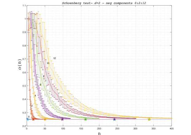
In this experiment we find that the critical value $\alpha_{0}$ is computed with an error $\approx 5\%$ for $n\approx 2(\ell_{\rm min}+1)^{2}$; these values are shown by the symbols $\star$ on the line at $\alpha=0.25$. It is clear that there is a systematic error for small $n$ which dominates the statistical error represented by the errorbars. In a real problem we do not know the value of $\ell_{\rm min}$, hence one has to compute at the highest value reachable for $n$ and one should try to extrapolate at infinite $n$.

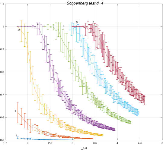
In the following two plots we report the same test performed for dimensions $d=3$ and $4$. The $x$-axis is scaled as $n^{1/3}$ and $n^{1/4}$, respectively, to make the plot more compact; this is based on the fact that a good range for $n$ starts at $2H(\ell_{\rm min},d)=O(\ell_{\rm min}^{d})$.

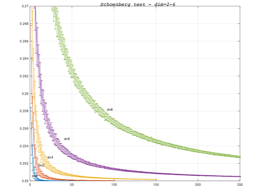
In Fig.6 we see many values of $d$ at the same time: also here the function is not the same, rather the coefficients of the expansion in hyperspherical polynomials are the same, and we see how convergence is slower in higher dimensions. To check Schoenberg test in all dimensions is obviously impossible, but here we see that the approximation improves with the number of vectors in the $n$-tuple.

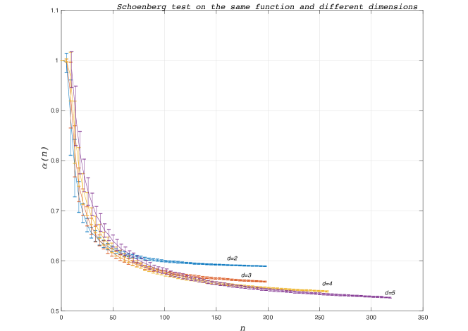
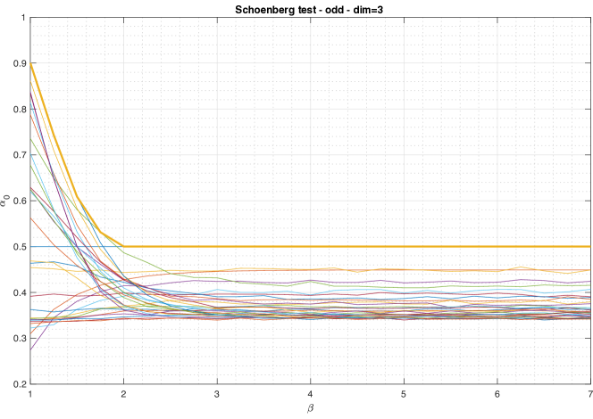
Finally in Fig.7 we report the result in the case of the same function tested in different dimensions. As expected the limiting values which approach the critical values of the parameter $\alpha$ are ordered in such a way that positivity in $d$ implies positivity in lower dimensions. This property applies to the limiting values, while there is no reason to expect that it apply to any value of the dimension of the $n$-tuples. We applied the technique based on Schoenberg’s theorem to the original problem of finding the positivity range for $\alpha_{0}$. A preliminary result is encouraging (see Fig.8). However, if applicable, the algebraic method is much more efficient. The alternative tecnique based on Schoenberg’s theorem may turn out to be the right choice in cases where an explicit analytic expression is not available for the function $f(x)$.

Appendix A The matlab code for Schoenberg’s test

We report here relevant parts of the code. The complete working code can be downloaded from the author’s website.

  ’SchoenbTest.m’    function [alpha, dalpha, setup, nout,Y] = SchoenbTest(setup)  % Schoenberg test. A number of n-tuples are extracted for  % each n in an interval fixed in setup. The mean and std over all runs  % is recorded. The output "alpha" contains the best  % estimate of alpha as a function of the cardinality n of n-tuples and  % dalpha gives the statistical error.  Y is a structure containing  % the data needed by the various subroutines. The main loop on sweeps  % is parallelized on the available cores (parfor)  %  % Usage:  %       [alpha, dalpha, setup, nout , Y] = SchoenbTestS([setup])if nargin<1,  setup = initialize();     % setup parameterelse   setup = initialize(setup);     % setup parameterendY.dim      = str2num(setup{1});samples  = str2num(setup{2});  % putting in Y all parameters to be passed to subroutinesY.tol        = str2num(setup{3});NN           = str2num(setup{4}); % interval for nY.a0         = str2num(setup{5}); % critical value of alphaY.nmax   = str2num(setup{6});hits          = str2num(setup{7});cf             = str2num(setup{8}); % expansion coefficientsrng(’shuffle’,’twister’)        % initialize random numbersY.cf  = cf;Y.cfP = zeros(size(cf));Y.cfP(hits) = Y.cf(hits); % selects coefficients dependent on alphaalpha  = zeros(length(NN),1);dalpha = zeros(length(NN),1);nout = zeros(length(NN),1);index = 1;for n = NN,   acum = zeros(samples,1);   parfor rep = 1:samples,                % parallelized loop      dim = Y.dim(1);      v = randn(dim,n);               % N vectors at random in R^{dim}      s = ones(dim,1)*sum(v.^2);      v = v./sqrt(s);      z = v’*v;                         % matrix v_i . v_j      a = bisec(z, Y, n);      acum(rep)=a;   end   nout(index) = n;   av = mean(acum);    dev = std(acum);   alpha(index)   = av; dalpha(index)  = dev;   index = index+1;end%------------------------------------------function a = bisec(z, Y, n)a1 = 0.0; a2 = 1.0;while(a2-a1 > Y.tol)   a = (a1+a2)/2;   flag = negeig(a, z, Y, n);   if flag,      a2 = a;   else,         a1 = a;   endend%%-------------------------------------------------function flag = negeig(a, z, Y, N)% sampling n-tuples on S^{dim-1} to study positivity of function F% defined below. Fires a flag when a negative eigenvalue is detected:flag = 0;warning offnu = Y.dim(2)/2-1;                       % parameter of Gegenbauer                                          % polyn. sph.harm. on S^(dim-1)C  = Y.cf;P  = Y.cfP;a0 = Y.a0;C0 = 1;              % Gegenbauer computed by recurrenceC1 = 2*nu*z;F  = C0*(C(1)-a/a0*P(1))*ones(size(z)); % P_0for k = 1:Y.nmax,   F = F + C1*(C(k)-a/a0*P(k));% P_{k+1}(z) ....   C2 = (2*(k+nu)*z.*C1 - (k-1+2*nu)*C0)/(k+1);<   C0 = C1;   C1 = C2;endF = F.*(ones(size(F)));F = 0.5*(F+F’);if(N<500),   ev  = min(eig(F));else   opts.issym = true;   opts.p = 40;   ev = eigs(F, 1, ’sr’, opts);endif(ev < 0),   flag = 1;end  % set flag and return%%----- setting up parameters via "inputdlg"function data = initialize(setup)% ......  instructions to set the parameters values interactivelydata = inputdlg(entries, title, lines, default, AddOpts); 

Figure 4. Schoenberg’s test at work: $\alpha_{0}=0.5$

Figure 5. Schoenberg’s test at work: $\alpha_{0}=0.5$

Figure 6. Exploring $n$-tuples in various dimensions at fixed parameters. $\alpha_{c}=0.25$.

Figure 7. Exploring $n$-tuples in various dimensions keeping the function $f(x)$ fixed.

Figure 8. Fig.2 reproduced by Schoenberg’s theorem.

References

- [1] G. Veneziano, S. Yankielowicz and E. Onofri, JHEP04 (2017) 151, ariv .
- [2] I. J. Schoenberg, Duke Math. J. 9(No.1) 1942
- [3] J. Stewart, Rocky Mountain J. Math. Volume 6, Number 3 (1976), 409-434.
- [4] C. Müller, Spherical Harmonics, Springer-Verlag (1966) (Lecture Notes in Mathematics).
- [5] H. Hochstadt, The functions of Mathematical Physics, Wiley-Interscience, New York 1971.
- [6] R.K. Beatson, W. zu Castell and Y. Xu, IMA J. Numer. Anal. (2014) 34 (2): 550-568.
- [7] G.H. Golub and J.H. Welsch, Math. Comput. 23 (1969) 221-230.
- [8] G.E. Andrews, R. Askey and R. Roy, “Special functions”, Cambridge U.P., 1999.