∎
Education, Science, and Technology of São Paulo
Caraguatatuba, São Paulo – Brazil
22email: venezian@ifsp.edu.br 33institutetext: L. Venezian Povoa 44institutetext: Aeronautics Institute of Technology
São José dos Campos, São Paulo – Brazil 55institutetext: C. Marcondes 66institutetext: H. Senger 77institutetext: Computer Science Department,
Federal University of São Carlos
São Carlos, São Paulo – Brazil
77email: {senger, marcondes}@dc.ufscar.br
Modelling Energy Consumption based on Resource Utilization
Abstract
Power management is an expensive and important issue for large computational infrastructures such as datacenters, large clusters, and computational grids. However, measuring energy consumption of scalable systems may be impractical due to both cost and complexity for deploying power metering devices on a large number of machines. In this paper, we propose the use of information about resource utilization (e.g. processor, memory, disk operations, and network traffic) as proxies for estimating power consumption. We employ machine learning techniques to estimate power consumption using such information which are provided by common operating systems. Experiments with linear regression, regression tree, and multilayer perceptron on data from different hardware resulted into a model with 99.94% of accuracy and 6.32 watts of error in the best case.
Keywords:
Computer architecture; Energy consumption modeling1 Introduction
Over the years, managing energy efficiency of Information and Communication Technologies (ICT) has increasingly emerged as one of the most critical environmental challenges. Due to ever increasing demand for computing resources, emissions footprint, increased energy price and tougher regulations, improving energy efficient became priority for datacenters, especially to the massive ones. This concern is pervasive in ICT, from development of more energy efficient devices to greener virtualization, resource consolidation, and, finally, definition of new architectures, services, and best practices.
In 2007, a Gartner’s Report showed that ICT industry generated 2% of global CO2 gartner_co2 emissions. From which, 23% came from datacenters. A Greenpeace’s report greenpeace stated that “datacenters are the factories of the 21st century in the Information Age”, however, they can consume as much electricity as 180,000 homes.
The constant reduction in computation resources prices, accompanied with popularization of on-line businesses, and wide spread of Internet and wireless networks, lead to the rapid growth of massive datacenters, consuming large amounts of energy. Indeed, nowadays, datacenters that execute Internet applications consume around 1.3% of the energy produced in the world gao2012s . It is expected in 2020 that this amount will rise to near 8% koomey2011growth . In such scenario, improving power efficiency on ICT installations and datacenters is mandatory. To overcome this challenge, several strategies have been proposed, such as resource consolidation orgerie_et_al_2010 ; lee_e_zomaya_2012 ; song_et_al_2009 , and improving resources utilization barroso_e_holzle_2007 .
In general, better energy efficiency can be achieved by means of actuation strategies which need the continuous power consumption measurement. The deployment of power meters may be prohibitive in terms of cost in datacenters with many thousands of computers. Furthermore, external metering instruments require physical system access or invasive probing song2013simplified , which can be not avaliable. On the other hand, software estimators for power consumption can be easily deployed at almost negligible cost.
An usual approach is to use internal performance counters provided by the hardware naveh2011power and by the operating system to derive models that estimate power consumption contreras2005power ; joseph2001run ; isci2003runtime ; bertran2010decomposable . Such models can be used by on-the-fly power saving strategies which need continuous power consumption estimation. Other possible applications include simulators that evaluate the power consumption of workloads based on performance and resource usage counters (e.g., register file usage, number of page faults, number of I/O operations per second).
In this paper, we propose models that use counter of both performance and resource utilization as proxies for power consumption. Differently from most of the related work, our models are not limited to predict power consumption of specific components, but of whole machine.
We assume a good model should include all performance counters which significantly influence the power consumption. However, the excess of parameters and non-linear relations between these variables and power consumption can produce complex and inaccurate models. Having this on mind, we also investigate which operating system counters can be used to build robust and accurate models.
In a previous work povoa2013model , we studied the correlation between a set of resource utilization counters provided by an operating system and the power consumption on a typical server machine. We also proposed a first-cut linear regression model with encouraging results.
Now, we further elaborate on correlation analysis and estimation of power consumption from resource utilization variables (i.e., counters) provided by operating systems. With this purpose, we apply nine models based on () Multiple Linear Regression (MLR), () Regression Tree (RET), and () Multilayer Perceptron (MLP), an Artificial Neural Network (ANN) which are experimentally evaluated on two different hardware 111The models were implemented in R (using RSNNS) and they are available under the GNU General Public License version 3 at https://github.com/lucasvenez/ecm along with the employed dataset.
The remainder of this paper is organized as follows. Section 2 describes the modeling approach, the workload, and the testbed used for experiments. Section 3 shows the collected variables and which of them have most impact on power consumption to be considered in the models. Section 4 describes the power consumption models based on the MLR, RET, and MLP methods. Section 5 presents accuracy and performance analysis of each proposed model. Section 6 presents some related work. Finally, Section 7 presents our final remarks.
2 Materials and Methods
This paper aims to provide a characterization of the power consumption for a wide variety of machines. With this purpose, we propose new models which provide accurate estimates for the power consumption based on resource utilization measurements commonly supported by the operating system used from commodity computers to datacenter servers. In this section, we describe the initial steps to develop such models.
2.1 Modelling Approach
In order to model power consumption for different computers, we employed a five-step method as depicted in Figure 1.
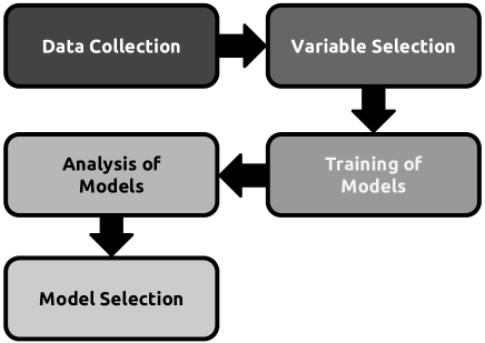
In Data Collection step, a synthetic workload is executed and an agent is used to collect data about resource utilization from the operating system iaee ; iaee_impl . The agent captures forty-seven variables from /proc directory. Second step is the Variables Selection, which aims to select variables that are influential to power consumption. We employed a correlation method called Maximal Information Coefficient (MIC) mine that evaluates the correlation of a pair variables regardless of the distribution. Next step, called Training of Models, aims to fed models with resource utilization samples and reads of the actual energy consumption measured in the testbed. Analysis of Models is the next step, in which focus on evaluating models accuracy through a set of different metrics. The final step is Model Selection, where the best estimation model for power consumption is selected.
2.2 Data Collection
Our objective is to characterize power consumption using operating system counters as proxies for energy consumption. We built a synthetic workload instead of using real applications or benchmarks aiming to conceive energy consumption models which are suitable for any application, while avoiding collinearity problems which may compromise regression models pazzani1999independent ; bertran2010decomposable .
The workload was designed to avoid cross dependency among the features fed to the model and produce all power consumption states for all system components such as memory, hard disk, processor, network interfaces and I/O da2010methodology . Workload was produced by using three open source tools: () stress stress was used to produce utilization of resources such as processor, memory, hard disk and input and output; () cpulimit cpulimit was used to generate random periods of idleness to produce several levels of processor utilization; and () iperf iperf to generate network traffic.
Workload was produced with the following characteristics. CPU utilization varied between 0% and 100% in several cycles, being increased in steps of 5% each. Each experiment was composed by processes with , where is the number of processors in the machine for the test. Memory utilization ranged from 512MB to the physical memory size. For the experiment, one application process allocates MB of memory, such that . Hard disk utilization varied from 1GB to 64GB, being produced by one process. For each experiment, the amount of disk space allocated is GB, where .
I/O workload was expressed by the number of processes that performed the message exchanges between the memory and the hard disk. The amount of processors exchanging messages was given by , with , where is the number of the experiment.
In the beginning, only one parameter was selected to vary for each experiment, in order to capture its influence on power consumption. Then, parameters were varied to test every all-to-all combinations of the several parameter levels, in order to capture their influence on power consumption and as well as parameter interactions. For each combination of parameters and level, the workload is executed for two minutes. The overall experiment took about fifteen hours to be carried out, producing about 51,000 entries, each entry containing measures from 29 variables of resources utilization and the power consumption.
2.3 Testbed Used for Experiments
The testbed used for experiments is depicted in Figure 2. Some cluster nodes were instrumented to measure power consumption while running workloads. We employed two nodes with different architectures in the experiments, which have their hardware configuration summarized in Table 1.
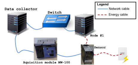
In order to obtain precise power consumption measures, we used a power sensor Yokogawa model 2375A10 2375a10 . This device works connected to the power supply, and provides data to one data acquisition module model MW-100-E-1D mw100 . The acquisition module probes and saves measures on power consumption in watts every 100 milliseconds. A software agent was implemented for collecting data from the acquisition module via a network interface using the telnet protocol.
| Hardware | A1 | A2 |
|---|---|---|
| Processor model | Intel Core i5-2400 | AMD Opteron 246 |
| Cores | 4 | 2 |
| Frequency | 3.10 GHz | 2.00 GHz |
| Memory | 4GB SDRAN | 8GB SDRAN |
| Disk | 1 500GB | 4 240GB |
3 Variables Selection
The design of accurate models depend upon a good selection of resource utilization counters 222Details about each independent variable considered in this paper are described in Supplementary Material. which present significant influence on power consumption and do not produce noise.
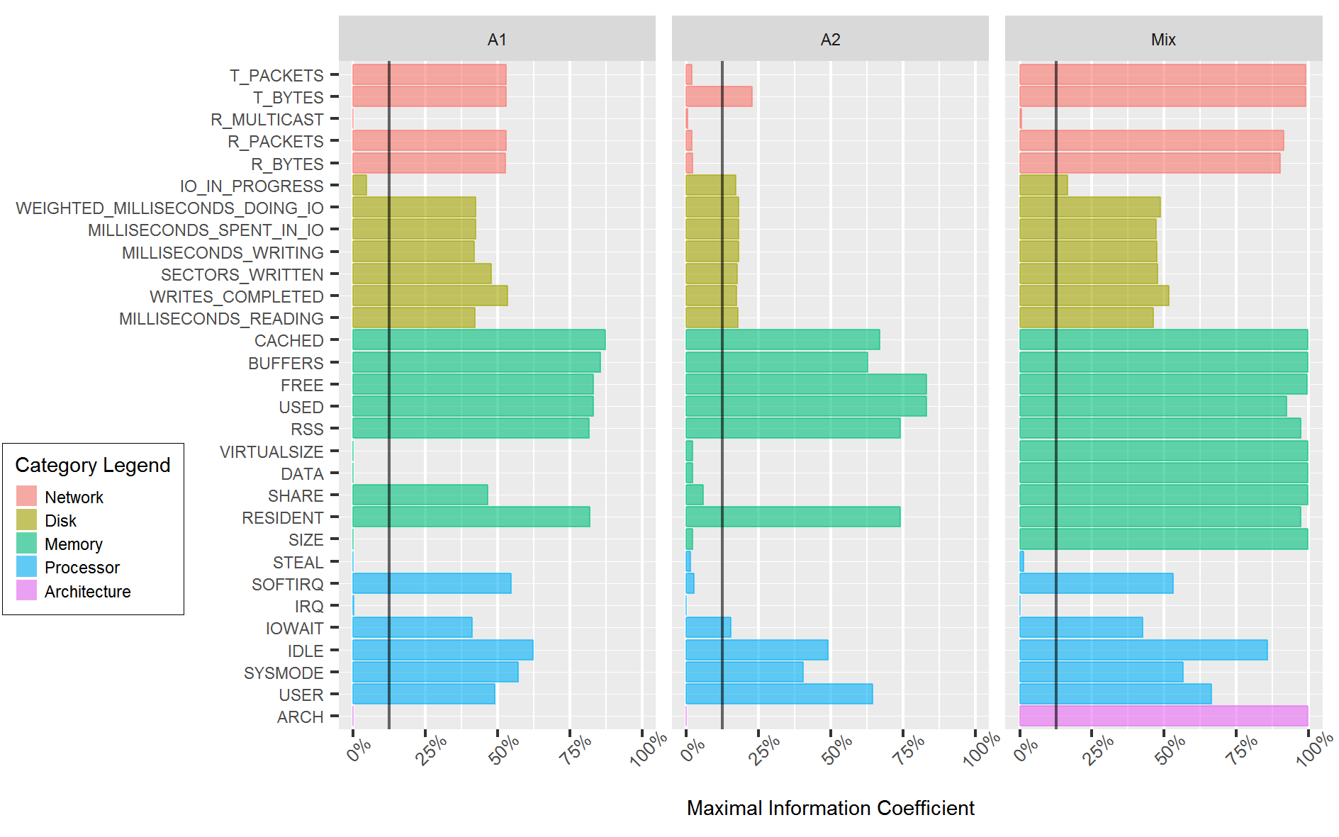
For the sake of clearness and understandability, a model for estimating energy consumption should be simple, i.e., to consider only a subset composed of the most influential variables on energy consumption. With this purpose, we identified from the set of observed variables, the subset with the highest correlation with the dependent variable (i.e., the energy consumption).
In order to evaluate correlation among variables, two main criteria should be considered. The first on is generality, which means capacity of identifying any relation type, not limited to specific types of correlation functions such as linear, exponential and periodic correlations, for instance. The later is equitability, that means the ability to provide a unique index to express relation with the same noise level, even for functions of different types.
Consequently, we chose a statistical method MIC to discover what are the most impacting variables for energy consumption. It is part of a set of tools named Maximal Information-based Nonparametric Exploration (MINE) mine . As result, MIC produces values between 0 and 1, where zero means absence of correlation between the pair of variables and 1 means full correlation.
Each architecture generated a dataset of the variables described previously. Based on these two datasets was generated a third one containing all data of both architectures, called Mix, joined to another variable, which determines whether the data is related to the architecture A1, described as -1, or to the architecture A2, described as 1.
Figure 3 shows results of the MIC between each independent variable, i.e., operating system’s variables, and the dependent variable, i.e., energy consumption. In the chart the vertical black line represents the threshold of 10%, which was applied with the purpose of finding a reduced set of the most impacting coefficients and produce a model with good understandability.
3.1 Dependent variable analysis
The distribution followed by the dependent variable of a model, which is the energy consumption our case, defines the method that can be used for modeling its behavior. The conventional Linear Regression method, for example, is not appropriated for modeling dependent variables that has no a Gaussian distribution.
Figure 4 shows the histogram of the energy consumption of each architecture, A1, A2, and Mix. Visually it is noteworthy that neither architecture have a normal distribution.
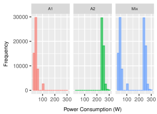
In order to confirm that power consumption do not present a Gaussian distribution we applied the Kolmogorov-Smirnov test ks-test for each architecture (A1, A2, and Mix). These tests resulted in p-values less than , which confirm that the dependent variable has no a Gaussian distribution considering a significance level of 5%.
The datasets A1, A2, and Mix present an average energy consumption (watts) of , , and , respectively. Their standard deviation are , , and . It is noteworthy that the architectures A1 and A2 have an stable energy consumption but in different ranges as also showed in Figure 4.
4 Models for Power Consumption
In this section we describe three models for estimating power consumption based on the most influential variables described in the previous Section.
4.1 Multiple Linear Regression Model
A MLR is a type of regression analysis that maps a set of input values to a response value , requiring that . However, as show in Section 3.1, neither datasets follow a normal distribution.
For dealing with this divergence, we consider the Central Limit Theorem (CLT), which states that when the size of a given sample increases, the sampling distribution of its average or sum tends to a normal distribution clt . Hence, the CLT justifies modelling the energy consumption with the MLR defined as
| (1) |
where
-
•
is the estimated value of the energy consumption;
-
•
is the intersection point of the line of adjustment with the ordinate;
-
•
is the regression coefficients vector;
-
•
is the independents variables vector; and
-
•
is the average random error.
This model employs the least-squares method for estimating the vector of coefficients , which is defined as
| (2) |
where
-
•
is the matrix of independent variable values; and
-
•
is the array of dependent variable values.
Figure 5 shows the model’s coefficient values for each architecture under analysis after applying Equation 2. The models for A1, A2, and Mix architectures have the intercept values , , and , respectively.
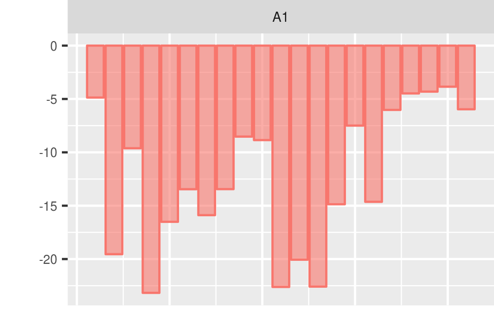
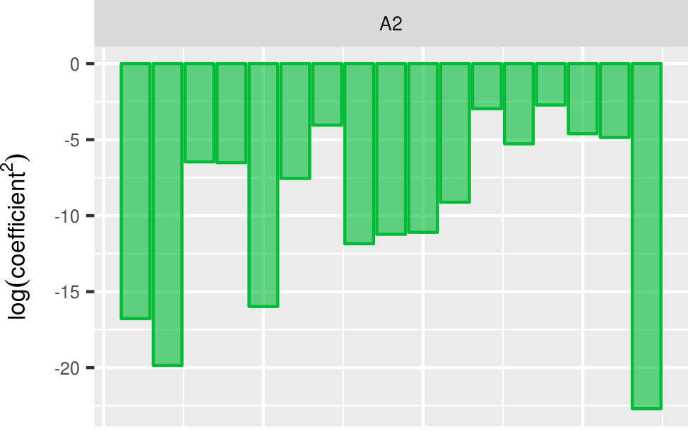
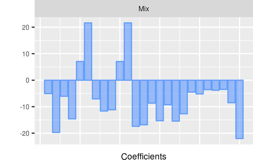
Despite the correlation analysis demonstrate high relation between the dependent variable and the independent variable labeled ARCH, the MRL method cannot incorporate this former into the resultant model for the Both dataset.
Despite of the high correlation analysis between the dependent variable and the independent variable ARCH, the MRL method cannot incorporate this former into the resultant model for the Both dataset. This is limitation for the MLR method for generating a global energy consumption model. A detailed analysis is presented in Section 5.1.
4.2 Regression Tree Model
A Decision Tree (DT) has a structure composed by leaves, branches and nodes aiming to define a nonlinear predictive model. A RET is a particular case of a DT, where values of dependent variables are continuous. Using a RET as predictor requires a sample be dropped down via the tree until a leaf, which returns the average of its values of the dependent variable CART .
A RET defines its configuration by splitting a node into two children nodes and . The split criterion of that is used to defined which variables gives the best split, is based on the sum of squared errors and defined in Equation 3 intro_rpart .
| (3) |
The tree stops to grow when the complexity index of a node is less or equals to a threshold . The complexity index of a node is calculated as follows:
| (4) |
where and are number of elements in the children nodes and , respectively.
For the experiments the threshold was set as . Applying our dataset of energy consumption in RETs generated the model illustrated in Figure 6.
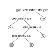
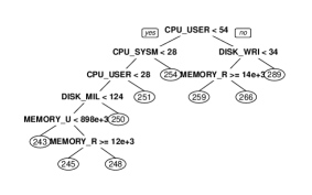
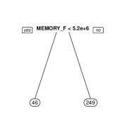
RET models are easy interpreted, but our results show that important variables are excluded for the model, which evidence a limitation of this method for modeling energy consumption. The resultant model for the Mix dataset represents our worst model, which considers only one independent variable for defining itself.
4.3 Multilayer Perceptron Model
A MLP is an Artificial Neural Network model that maps a set of input values into a set of output values mlp after a learning process. Recently, it is being successfully applied in different areas, e.g., Biometrics mlp_biometric , Thermal Engineering mlp_thermal , Ocean Engineering mlp_ocean , Climatology mlp_climatology .
The MLP is composed by an input layer with sensory units, hidden layers with neurons each, and an output layer with neurons. A MLP has layers, excluding the input layer, and its input values are propagated layer-by-layer. Figure 7 shows the general structure of this model.
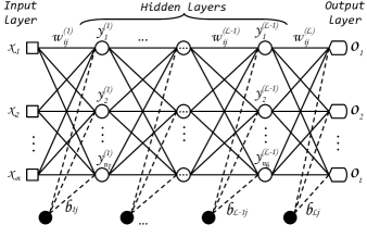
The neuron at layer has an induced local field defined by:
| (5) |
where
-
•
is the number of neurons at layer ;
-
•
is the weight between the neuron at layer and the neuron at layer ;
-
•
is the value of the neuron at antecedent layer ; and
-
•
is a bias at layer connected to neuron .
Each neuron is a computational unit composed by an input signal, a weight, and a nonlinear activation function. The output value for neuron at layer is denoted by
| (6) |
where is an activation function.
If neuron is located at layer , its output value . The output value for neuron at layer is denoted thought the variable .
The MLP’s learning process can be supervised or unsupervised. Once we collected both the input and output variables, this research applied the supervised learning process, i.e. a process that uses the expect output for correcting the model’s weights. The supervised learning process was performed with the backpropagation algorithm with chunk update, which has the following steps:
-
1.
forward step, where a set of input values is provided to the sensory units, and its effect is propagated layer-by-layer; and
-
2.
backward step, where the weights are adjusted in accordance with an error-correction rule respecting the Mini-Batch Stochastic Gradient Descent method minibatch after (chunk size) executions of the forward step.
The forward step applies Equation 6 for each neuron in each hidden layer . After that, an error signal related to neuron at output layer is denoted by:
| (7) |
where is the element of the desired response vector.
The backward step starts by computing the local gradient related to neuron at output layer according to:
| (8) |
When neuron is located at a hidden layer , the local gradient related to neuron at hidden layer is defined in by
| (9) |
where
-
•
is the derivative of ; and
-
•
is the number of neurons at layer .
The new value for the weight at layer is defined according to
| (10) |
where
-
•
is the iteration number, such that or ;
-
•
;
-
•
is the chunk size; and
-
•
is the learning-rate.
For setting the MLP’s configuration for each architecture, we applied an empirical method that consists of:
-
1.
selecting a random and non-sequential subset of registers from our sample, approximately of all registers;
-
2.
starting the model weights with a random Gaussian distribution with values between and ;
-
3.
ranging the number of hidden layers from until a descendant precision of the model;
-
4.
ranging the number of neurons at each layer from to , where is the number of independent variables at the model;
-
5.
ranging the learning-rate from to by ; and
-
6.
calculating the model precising using the Coefficient of Determination R2 metric for each possible configuration considering previous steps.
After finding the better combination for each architecture, where better combination refers to the one that results in the greatest R2, we applied the full sample for the learning process. In our study, the better configuration for the MLP consists of 3 hidden layers, where each one has the number of nodes equals to double of the number of input variables, a learning rate , and a chunk size . As activation function we used the function defined in Equation 11.
| (11) |
where is the Euler’s number.
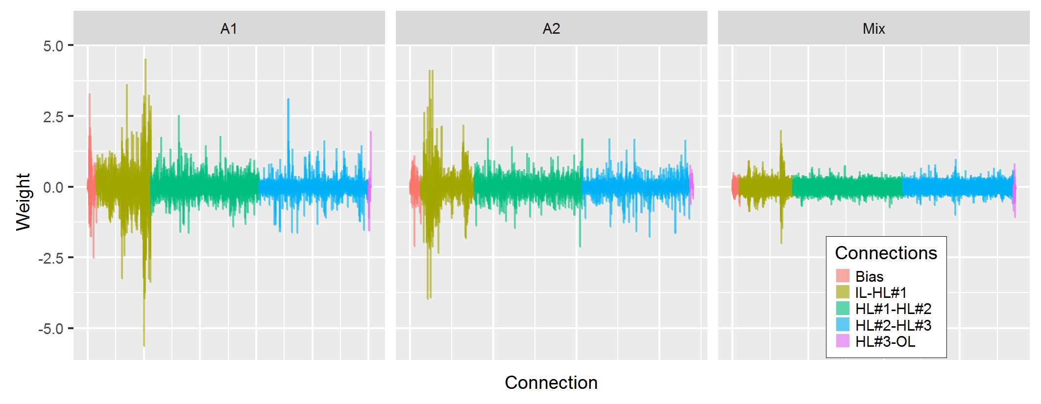
Figure 8 shows the models’ weights for each architecture under analysis after the learning process. The MLP models incorporate all independent variables with a relevant correlation to the dependent variable, which indicates MLP is acceptable for generating a global model for energy consumption.
5 Evaluating the proposed models
In this section, the power consumption models proposed in previous sections are evaluated both in terms of their accuracy and computational cost. For this purpose, different metrics and the 10-fold cross-validation (CV) method were employed.
5.1 The accuracy of the models
In order to evaluate the accuracy of each model, we applied four different classes of metrics: scale-dependent, percentage error, relative error, and scale-free error metrics mape .
Scale-dependent metrics are simple to understand and calculate, but cannot be applied to compared models of series with different scales. Percentage error metrics are scale independent, overcoming the limitations of scale dependent metrics. However, such metrics return infinite or undefined values when zeroes exist within the series. Relative error metrics are also scale independent metrics but they are restricted to some statistic methods when errors are small. Finally, scale-free error metrics never provide infinite or undefined values, and they can be applied to compare different estimate methods either over a single or multiple series.
In this paper, we used six metrics to evaluate our methods in order to ease future comparison with other methods. The first metric used is Squared Error (SE) given by:
| (12) |
where is the observed value, and is the estimate value.
The second metric is the Absolute Error (AE), which is defined by:
| (13) |
Although these two metrics are scale-dependent, they are used in related literature, such as in povoa2013model ; piga-2013 . The Percentage Error (PE) mape is a metric given by the ratio between the difference:
| (14) |
In this metric, positive and negative values can cancel each other, leading the average to approach to zero. The Absolute Percentage Error (APE) mape is another percentage error metric like PE, except by absolute function as defined by:
| (15) |
The Absolute Scaled Error (ASE) mase is a scale-free error metric, which is frequently used to measure the estimation accuracy. ASE avoids the common problems in conventional accuracy metrics described previously. It is defined as:
| (16) |
where is the sample size.
For the above mentioned metrics, the closer are the results to zero, the more accurate are the models. Another metric is R2, given by:
| (17) |
This metric show how well the estimated values produced by a model fit the actual ones. The result lies between 0 and 1, where 0 means the model does not provide any explanation about the data, and 1 refers to a perfect adjust.
| Average | Standard Deviation | |||||||||||
|---|---|---|---|---|---|---|---|---|---|---|---|---|
| Arch. | Method | SE | AE | PE | APE | ASE | SE | AE | PE | APE | ASE | R2 |
| A1 | MLR | 7.2878 | 1.6858 | -0.4008% | 3.8598% | 1.2426 | 56.1252 | 2.1064 | 5.6912% | 4.1994% | 1.5532 | 96.8650% |
| RET | 14.8066 | 2.8970 | -0.7901% | 6.8144% | 2.1249 | 54.7590 | 2.5281 | 8.9543% | 5.8610% | 1.8534 | 93.6364% | |
| MLP | 6.1053 | 1.4895 | 0.0332% | 3.3382% | 1.1040 | 56.3053 | 1.9594 | 5.1738% | 3.9961% | 1.4517 | 97.3777% | |
| A2 | MLR | 4.9962 | 1.3446 | -0.0078% | 0.5332% | 2.2536 | 21.4396 | 1.7845 | 0.8705% | 0.6880% | 2.9887 | 91.6575% |
| RET | 4.8958 | 1.3094 | -0.0067% | 0.5164% | 2.2015 | 20.3679 | 1.7828 | 0.8573% | 0.6844% | 2.9973 | 91.8226% | |
| MLP | 3.7707 | 1.1169 | -0.0115% | 0.4424% | 1.8725 | 18.0375 | 1.5873 | 0.7533% | 0.6115% | 2.6572 | 93.7082% | |
| Mix | MLR | 14.0595 | 2.6209 | -0.4336% | 3.7864% | 2.5888 | 53.7892 | 2.6807 | 5.9828% | 4.6517% | 2.6474 | 99.8654% |
| RET | 150.7207 | 7.7339 | -4.1102% | 11.7914% | 7.6287 | 533.8658 | 9.5315 | 19.3902% | 15.9341% | 9.4011 | 98.5565% | |
| MLP | 6.3264 | 1.5471 | -0.3946% | 2.3506% | 1.5232 | 48.7559 | 1.9796 | 4.3027% | 3.6313% | 1.9479 | 99.9394% | |
The metrics described above provide values closer to for better models and far from for worse ones. The PE metric can provide either negative and positive values, and the remainder metrics result only in positive values.
Next, the accuracy of each proposed model is evaluated applying the 10-fold cross validation method cv . For each test, the estimated value for the power consumption is compared to the actual measured value. Table 2 presents the average and standard deviation for the six metrics. All models presented . In particular, MLR models have low average errors for all metrics considering A1 and A2 architectures. However, when MLR is applied to fit the mix of architectures into a unique model, the error increases significantly. A similar effect occurs with RET models, whose accuracy is even worse than MLR models for the mix of architectures.
MLP models presented the best accuracy from the experiments. However, MLR are simpler and less costly models whose accuracy approach the MLP’s accuracy. It suggests non-linear relations with low significance between the independent variables and the dependent one. This evidence is supported by the the average and standard deviation, which are close but not equal.
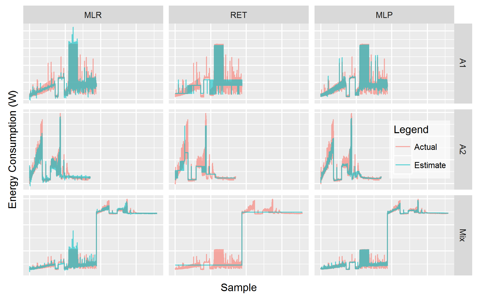
Noticeably, RET models present the worst accuracy from the three models. This can be explained as RET clusters data before estimating the power consumption. Indeed, power consumption cannot be explained for a small subset of dependent variables. However, all of the variables provide enough information for estimating power consumption, which hinders the clustering.
As depicted in Figure 9, the estimated and actual power consumption are close. Considering the results, we can conclude the MLP models provide better estimations for power consumption, while MLR are simpler models which present similar performance in terms of accuracy. Furthermore, experimental results also show that RET models do not provide accurate estimations for power consumption when compared to MLP and MLR models, mainly when dealing with mixed architectures in the same estimator.
5.2 Computational cost
Besides accuracy, computational cost to estimate power consumption is also assessed. All the three methods have a training phase and the application phase. During the training phase the method is fed with traces of operating system variables and actual power consumption reads from a meter, and calibrates its internal parameters to produce accurate estimates. Usually, the training phase is far more computationally expensive than the application phase. Table 3 shows the execution times (in minutes) for the training phase of each method. Executoin times were obtained with the GNU time tool time .
MLR presents the fastest training phase, around minutes. Not surprisingly, MLP is the slowest one (around 6.7 days). In general, such models will be trained once for each particular architecture profile. Machines with similar architecture can reuse the same model.
| A1 | A2 | Mix | |
|---|---|---|---|
| MLR | 0.81 | 0.65 | 2.69 |
| RET | 5.48 | 5.50 | 5.58 |
| MLP | 3,693.26 | 2,446.07 | 9,738.97 |
During the application phase, the model fed with an array of measures of resources utilization collected from the operating system and produces an estimate of power consumption. This is a computationally low cost operation that requires a few dozens of floating-point operations. Depending on the frequency that such calculation need to be executed (e.g. once a second), its computational cost may be negligible (far less than 1% of cpu utilization).
6 Related Work
A large number of papers has been published on modeling computers power consumption, including some surveys reda2012power ; orgerie2014survey ; model_survey . Several models have been proposed to estimate the energy consumption of processors joseph2001run ; contreras2005power ; bertran2013systematic ; bertran2010decomposable . Most of them consist of linear regression-based models which are fed with hardware performance counters. In isci2003runtime , a model was proposed combining real total power measurement with hardware counters measurement to estimate per-component energy consumption. Our approach is different from those works because our goal is to estimate energy consumption for the entire machine, not limited to the processor.
Other papers address the modeling of the entire computer (e.g., from commodity computers to datacenter servers) proposing linear models composed by the summation of the energy consumed by its subcomponents lewis2008run ; orgerie2012energy ; xiao2013virtual ; lent2013model . For instance, Lewis et al. lewis2008run propose an aggregated model which considers CPU, memory, electromechanical components, peripherals, and hard disk consumption. The models have coefficients for each component that are adjusted using linear regression. The energy consumed by virtual machines is also modeled in xiao2013virtual . Other non linear models are also proposed for modeling the entire computer energy consumption fan2007power ; tang2011dynamic . Our work is different as our objective is not to model energy consumption of the computer as an explicit summation of the consumption of its subcomponents. Instead, our models are fed with system variables carefully selected (by their ability to explain the model) in order to estimate energy consumption with high accuracy. Also, our work propose and compare models based on three different techniques.
As mentioned, regression models are numerous for modeling energy consumption. For instance, Piga piga-2013 defined a global center-level approach to power and performance optimization for Web Server Datacenters. Their model is based on linear and non-linear regression techniques, while using the k-means to identify non-linear correlation and the Correlation-based Feature Selection (CFS) for removing independents variables that do not provide significant explanation for the power consumption. Our focus, instead is to model individual computers based on observable operating system measures.
Da Costa et al. da2010methodology modeled computer energy consumption based on performance counters provided by two tools (Linux pidstat and collectd). The paper describes the methodology for reducing from a set of 165 explanatory variables to a small number of variables which can explain the model with high accuracy. The model is intended to estimate energy consumption at process level. Our work is different regarding the variety of techniques used, and modeling the whole machine energy consumption.
Comparing our models with the best related work results, considering the absolute percentage error, our best MLP specific and global models presented an error rate of 2.35%, and 0.44%, correspondingly, while lewis2008run ; piga-2013 ; da2010methodology ; dhiman have an error rate of , , , and , respectively.
We did not compare our models against all related work once some models have no direct correlation with our approach, measuring, for example, energy consumption of a specific hardware component or a whole data center, or providing an abstract model evaluation.
By the best of our knowledge, our work provides the following novel contribution: () propose and compare three different models to estimate the power consumption for more than one hardware configuration; () employ the MIC method to analysis the correlation between independent variables and the power consumption variable; () the proposed models are fed with commodity system variables commonly provided by Linux, for better portability; () accuracy analysis using several metrics along with cross-validation in order to verify precision and overfitting issues.
7 Conclusion
This paper presented a characterization of energy consumption of entire machines based on resources utilization variables. Experiments were carried out using synthetic workloads in order to discover what resources and modeling methods present higher correlation to energy consumption. We show that it is possible to estimate energy consumption by sampling variables provided by common operating systems and employing MLR, RET, or MLP methods. We proposed nine models that provide accurate estimation on energy consumption with an accuracy of 99.9%, and average squared error of watts with standard deviation of .
All models evaluated can be fully implemented in software, providing a cost-effective mechanism for estimating energy consumption. Such models can be deployed from a single machine to all machines in a large datacenter at no cost and negligible overhead. Our proposal can be useful for several aims, e.g., to provide instant information on energy consumption in a per machine basis in a datacenter. Such information can be consumed by management tools to provide accurate views of energy efficiency of the datacenter. Also, resource schedulers and consolidation tools could benefit from our proposal on different environments such as high performance clusters and cloud infrastructures.
Acknowledgements.
Authors thank CAPES and RNP for partially supporting this research project. Hermes Senger thanks CNPq (Contract Number 305032/2015-1) for their support. The authors declare that no funding body played any role in the design or conclusion of this study.References
- (1) Gartner, Gartner energy & utilities it summit 2007: an invitation only event. Tech. rep., Gartner, Dallas, EUA (2007)
- (2) G. Cook, How clear is your cloud? catalysing an energy revolution. Tech. rep., Greenpeace International, Amsterdam, The Netherlands (2012). URL http://goo.gl/yd1FAS
- (3) P.X. Gao, A.R. Curtis, B. Wong, S. Keshav, in Proceedings of the ACM SIGCOMM 2012 Conference on Applications, Technologies, Architectures, and Protocols for Computer Communication (ACM, New York, NY, USA, 2012), SIGCOMM ’12, pp. 211–222
- (4) J. Koomey, Growth in data center electricity use 2005 to 2010, vol. 1 (Analytics Press, Oakland, CA, 2011)
- (5) A.C. Orgerie, M. Assunção, L. Lefèvre, in Grids, Clouds and Virtualization, ed. by M. Cafaro, G. Aloisio, Computer Communications and Networks (Springer London, 2011), pp. 143–166
- (6) Y. Lee, A. Zomaya, The Journal of Supercomputing 60, 268 (2012)
- (7) Y. Song, H. Wang, Y. Li, B. Feng, Y. Sun, in CCGRID 0́9. (2009), pp. 148 –155
- (8) L.A. Barroso, U. Hölzle, Computer 40(12), 33 (2007)
- (9) S. Song, C. Su, B. Rountree, K.W. Cameron, in Parallel & Distributed Processing (IPDPS), 2013 IEEE 27th International Symposium on (IEEE, 2013), pp. 673–686
- (10) A. Naveh, D. Rajwan, A. Ananthakrishnan, E. Weissmann, in Hot Chips (2011)
- (11) G. Contreras, M. Martonosi, in Low Power Electronics and Design, 2005. ISLPED’05. Proceedings of the 2005 International Symposium on (IEEE, 2005), pp. 221–226
- (12) R. Joseph, M. Martonosi, in Proceedings of the 2001 international symposium on Low power electronics and design (ACM, 2001), pp. 135–140
- (13) C. Isci, M. Martonosi, in Proceedings of the 36th annual IEEE/ACM International Symposium on Microarchitecture (IEEE Computer Society, 2003), p. 93
- (14) R. Bertran, M. Gonzalez, X. Martorell, N. Navarro, E. Ayguade, in Proceedings of the 24th ACM International Conference on Supercomputing (ACM, 2010), pp. 147–158
- (15) L. Venezian Povoa, P. Bignatto Junior, C. Monteiro, D. Mueller, C. Marcondes, H. Senger, in IEEE Symposium on Computers and Communications (ISCC) (IEEE Computer Society, 2013), pp. 1–6
- (16) P.M. Dusso, A monitoring system for wattdb: An energy-proportional database cluster. Graduation thesis, Informatics Institute, Federal University of Rio Grande do Sul, Porto Alegre, Brazil (2012). URL http://goo.gl/8gheFW
- (17) P.M. Dusso. energyagent (2012). URL https://github.com/pmdusso/energyagent
- (18) D.N. Reshef, Y.A. Reshef, H.K. Finucane, S.R. Grossman, G. McVean, P.J. Turnbaugh, E.S. Lander, M. Mitzenmacher, P.C. Sabeti, Science 334(6062), 1518 (2011)
- (19) M.J. Pazzani, S.D. Bay, in Proceedings of the Twenty-First Annual Meeting of the Cognitive Science Society (1999), pp. 525–530
- (20) G. Da Costa, H. Hlavacs, in 2010 11th IEEE/ACM International Conference on Grid Computing (IEEE, 2010), pp. 290–297
- (21) A. Waterland. stress (2014). URL http://people.seas.harvard.edu/~apw/stress/
- (22) A. Marletta. cpulimit (2012). URL https://github.com/opsengine/cpulimit
- (23) NLANR/DAST. Iperf - the tcp/udp bandwidth measurement tool (2011). URL https://iperf.fr/
- (24) Yokogawa Electric Corporation, 0.5 Class Transducer for Power Application (2009). URL http://goo.gl/f43ZwV
- (25) Yokogawa Electric Corporation, Data Acquisition Unit MW100 (2013). URL http://goo.gl/7mcNV8
- (26) G. Marsaglia, W.W. Tsang, J. Wang, Journal of Statistical Software 8(18), 1 (2003)
- (27) J.R. Rice, Mathematical Statistics and Data Analysis (Thomson Books/Cole, United States of America, 2007), 3rd edn., chap. 5 - Limit Theorems
- (28) L. Breiman, J. Friedman, C.J. Stone, R. Olshen, Classification and Regression Trees (Chapman and Hall, New York, USA, 1984)
- (29) T.M. Therneau, E.J. Atkinson, An introduction to recursive partitioning using the rpart routines. Tech. rep., The R Foundation (2015). URL https://goo.gl/YmMfNb
- (30) S. Haykin, Neural Networks: A Comprehensive Foundation, 2nd edn. (Prentice Hall, 1998)
- (31) V.B. Semwal, M. Raj, G. Nandi, Robotics and Autonomous Systems 65, 65 (2015). DOI 10.1016/j.robot.2014.11.010
- (32) M. De Lozzo, P. Klotz, B. Laurent, Engineering Applications of Artificial Intelligence 26(10), 2270 (2013). DOI 10.1016/j.engappai.2013.07.001
- (33) A. Altunkaynak, Ocean Engineering 58, 144 (2013). DOI 10.1016/j.oceaneng.2012.08.005
- (34) R. Velo, P. López, F. Maseda, Energy Conversion and Management 81, 1 (2014). DOI 10.1016/j.enconman.2014.02.017
- (35) M. Li, T. Zhang, Y. Chen, A.J. Smola, in Proceedings of the 20th ACM SIGKDD International Conference on Knowledge Discovery and Data Mining (ACM, New York, NY, USA, 2014), KDD ’14, pp. 661–670. DOI 10.1145/2623330.2623612
- (36) R.J. Hyndman, A.B. Koehler, International Journal of Forecasting pp. 679–688 (2006)
- (37) L. de Paula Rosa Piga, Modeling, characterization, and optimization of web server power in data centers. Ph.D. thesis, Institute of Computing (IC), University of Campinas (UNICAMP), Campinas, Brazil (2013)
- (38) R.J. Hyndman, Foresight: The International Journal of Applied Forecasting (4), 43 (2006)
- (39) R. Kohavi, in Proceedings of the 14th International Joint Conference on Artificial Intelligence - Volume 2 (Morgan Kaufmann Publishers Inc., San Francisco, CA, USA, 1995), IJCAI’95, pp. 1137–1143
- (40) D. MacKenzie, GNU time 1.7 (2010). URL http://goo.gl/QYPqN3
- (41) S. Reda, A.N. Nowroz, Foundations and Trends in Electronic Design Automation 6(2), 121 (2012)
- (42) A.C. Orgerie, M.D.d. Assuncao, L. Lefevre, ACM Computing Surveys (CSUR) 46(4), 47 (2014)
- (43) M. Dayarathna, Y. Wen, R. Fan, IEEE Communications Surveys Tutorials 18(1), 732 (2016). DOI 10.1109/COMST.2015.2481183
- (44) R. Bertran, M. Gonzalez, X. Martorell, N. Navarro, E. Ayguade, IEEE Transactions on Computers 62(7), 1289 (2013)
- (45) A.W. Lewis, S. Ghosh, N.F. Tzeng, HotPower 8, 17 (2008)
- (46) A.C. Orgerie, L. Lefèvre, I. Guérin-Lassous, The Journal of Supercomputing 62(3), 1139 (2012)
- (47) P. Xiao, Z. Hu, D. Liu, G. Yan, X. Qu, Journal of Network and Computer Applications 36(2), 818 (2013)
- (48) R. Lent, Sustainable Computing: Informatics and Systems 3(2), 80 (2013)
- (49) X. Fan, W.D. Weber, L.A. Barroso, in ACM SIGARCH Computer Architecture News (ACM, 2007), pp. 13–23
- (50) C.J. Tang, M.R. Dai, in System Integration (SII), 2011 IEEE/SICE International Symposium on (IEEE, 2011), pp. 1159–1164
- (51) G. Dhiman, K. Mihic, T. Rosing, in Design Automation Conference (DAC), 2010 47th ACM/IEEE (2010), pp. 807 – 812. DOI 10.1145/1837274.1837478