Probing the anomalous dynamical phase in long-range quantum spin chains through Fisher-zero lines
Abstract
Using the framework of infinite Matrix Product States, the existence of an anomalous dynamical phase for the transverse-field Ising chain with sufficiently long-range interactions was first reported in [J. C. Halimeh and V. Zauner-Stauber, arXiv:1610:02019], where it was shown that anomalous cusps arise in the Loschmidt-echo return rate for sufficiently small quenches within the ferromagnetic phase. In this work we further probe the nature of the anomalous phase through calculating the corresponding Fisher-zero lines in the complex time plane. We find that these Fisher-zero lines exhibit a qualitative difference in their behavior, where, unlike in the case of the regular phase, some of them terminate before intersecting the imaginary axis, indicating the existence of smooth peaks in the return rate preceding the cusps. Additionally, we discuss in detail the infinite Matrix Product State time-evolution method used to calculate Fisher zeros and the Loschmidt-echo return rate using the Matrix Product State transfer matrix. Our work sheds further light on the nature of the anomalous phase in the long-range transverse-field Ising chain, while the numerical treatment presented can be applied to more general quantum spin chains.
I Introduction
Equilibrium phase transitions are a hallmark of statistical mechanics and condensed-matter physics. They are well-understood textbook subjects that have been treated through various theories. From Landau’s theory of symmetry breaking Cardy ; Sachdev that presents an intuitive field-theoretical approach built upon the symmetries of the model under consideration to Wilson’s renormalization group Fisher1974 that utilizes scale invariance, the theoretical description of equilibrium phase transitions has been validated in numerous experiments, not the least in quantum many-body systems. Nevertheless, the field of dynamical phase transitions, particularly in quantum many-body systems, is still in its infancy, and much is left unanswered.
One of the most interesting notions of dynamical criticality in quantum many-body systems in the thermodynamic limit is that manifested in non-analyticities in the Loschmidt-echo return rate Heyl2013 ; Heyl2015 of a quenched system. We have termed this type of dynamical phase transition as DPT-II Halimeh2016b , in contrast to dynamical phase transitions defined in terms of dynamical order parameters (DPT-I). One of the paradigmatic models of statistical mechanics, the one-dimensional transverse-field Ising model (TFIM), has been the bulwark of investigations of the DPT-II in its nearest-neighbor (NN-TFIM) Heyl2013 ; Heyl2015 and long-range interacting (LR-TFIM) Zunkovic2016 ; Zunkovic2016b ; Halimeh2016b ; Halimeh2017 variants. For short-range interactions the Loschmidt-echo return rate displays cusps for quenches across a dynamical critical point (regular phase) and no cusps otherwise (trivial phase), where for nearest-neighbor interactions in particular the equilibrium and dynamical critical points coincide Heyl2013 ; Zunkovic2016b ; Halimeh2016b . With sufficiently long-range interactions, however, the Loschmidt-echo return rate shows cusps also for quenches within the equilibrium ordered phase that do not cross the dynamical critical point, with these cusps being of a different nature Halimeh2016b ; Halimeh2017 .
In particular, considering in the case of long-range interactions only quenches from an ordered initial state, it has been shown in Refs. Halimeh2016b, ; Halimeh2017, that the Loschmidt-echo return rate displays anomalous cusps for quenches below the dynamical critical point (which in this case does not coincide with the equilibrium critical point), whereas for quenches above it, the traditional regular cusps familiar from the NN-TFIM case are present. Besides other qualities distinguishing the anomalous cusps from their regular counterparts, the defining feature of the anomalous phase is that the Loschmidt-echo return rate displays cusps only after its first minimum. Especially for small quenches these cusps typically only appear at rather late times after a number of preceding smooth peaks. Moreover, at least in the limit the anomalous (regular) phase coincides with a finite (zero) long-time average of the order parameter Halimeh2017 .
In this paper we seek to shed more light on the qualitative difference between the anomalous and regular cusps, in particular in terms of Fisher zeros, as computed in the framework of infinite Matrix Product States (iMPS). Much like the Lee-Yang analysis of equilibrium phase transitions in the complex external-magnetic-field plane Yang1952 ; Lee1952 where a phase transition exists only if Lee-Yang zeros (or more specifically, the Lee-Yang singularity edges Kortman1971 ; Fisher1978 ) cross the positive real axis in the thermodynamic limit, the partition function is an entire function in the complex temperature plane Fisher1965 where Fisher zeros cross the real axis at a phase transition in the thermodynamic limit. Fisher zeros in the context of the DPT-II were first discussed in Ref. Heyl2013, , where it was shown that Fisher zeros cut the time axis, i.e. a dynamical phase transition exists, when the quench is across the equilibrium critical point in the case of the NN-TFIM. However, the equilibrium critical point is not always the dynamical critical point Andraschko2014 ; Vajna2014 , and the latter departs further from the former with increased range of interactions in the LR-TFIM Zunkovic2016b ; Halimeh2016b ; Halimeh2017 .
The paper is organized as follows: In Sec. II we discuss in some detail the workings of the iMPS method and its use in calculating our results. In Sec. III we present the Fisher-zero data, and discuss the qualitative difference between the anomalous and regular cases. In Sec. IV we discuss the existence of double cusps in the anomalous phase and we illustrate the crossover between the anomalous and regular phases around the dynamical critical point, both in terms of the level crossings of the rate-function branches of the Matrix Product State (MPS) transfer matrix. We conclude in Sec. V.
II Infinite Matrix Product State technique
As shown in the seminal works Heyl2013 ; Heyl2015 for the NN-TFIM, a DPT-II manifests itself as non-analyticities in the form of cusps in the Loschmidt-echo return rate. Due to finite-size effects, these cusps will be smoothened out in finite systems, thus indicating no non-analyticity (and thus no criticality) in the Loschmidt-echo return rate. One can in principle employ conventional MPS time-evolution techniques for finite-size systems TEBD_supp ; tDMRG1_supp ; tDMRG2_supp and use finite-size scaling in order to surmise a cusp in the thermodynamic limit, but such a procedure might be error-prone, cumbersome, and requires unrealistic numerical resources. It is therefore desirable to perform simulations directly in the thermodynamic limit, which can be done very efficiently using iMPS MPS1_supp ; MPS2_supp ; Uli_supp without any approximations in addition to using Matrix Product State representations. One can then directly see sharp cusps in the Loschmidt-echo return rate, which are due to level crossings in the eigenvalues of the MPS transfer matrix (see below). This constitutes an additional advantage over a finite-size-scaling approach, where it can be very unclear if a maximum in the return rate will develop into a non-analytic cusp in the limit of infinite system size. In the case of iMPS, due to translation invariance, the presence or absence of level crossings in the spectrum of a single MPS transfer matrix is a clear indicator of the occurrence of non-analytic cusps.
Conventional techniques for MPS time evolution in the thermodynamic limit ITEBD_supp relying on an efficient Trotter-Suzuki decomposition Trotter_supp ; Suzuki_supp of the time-evolution operator can be employed for long-range interacting systems, however only by introducing additional approximations Pollmann2015_supp . MPS tangent-space methods based on the time-dependent variational principle (TDVP) TDVP_supp ; MPS_tangent_supp ; TDVP_Uni_supp on the other hand directly integrate the time-dependent Schrödinger equation within the variational manifold of MPS and therefore only require the application of the Hamiltonian onto an MPS, thus avoiding an approximate Trotter-Suzuki decomposition of .
In order to efficiently apply a Hamiltonian with (e.g. decaying power-law) long-range interactions onto an MPS, we expand it in a sum of exponentially decaying interaction terms, which we outline in Sec. II.1. We then describe the algorithm we use to simulate the real-time evolution of a pure state on a spin chain under such a Hamiltonian in the thermodynamic limit in Sec. II.2. In Sec. II.3 and Sec. II.4 we finally describe how to efficiently calculate the Loschmidt-echo return rate in the framework of iMPS and how non-analyticities in the form of cusps naturally arise due to level crossings in the (mixed) MPS transfer matrix arising in the overlap between the time-evolved and initial states.
II.1 Long-range interactions
We assume the Hamiltonian to contain a sum of two-body interactions of the form , where operators act on a single site and commute when acting on different sites . Specifically, we consider the long-range transverse-field Ising model
| (1) |
where are Pauli matrices acting on site , is the spin-spin coupling constant, is the transverse magnetic field, and is the number of sites. We consider the thermodynamic limit . The distance function decays as a power law and we assume to be well approximated Crosswhite2008 by a sum of exponentials, i.e. , with and . With this approximation the overall Hamiltonian is then given by
| (2) |
For an infinite system we perform a non-linear least-squares fit of with a suitable number of exponentials over a distance large enough such that , where is of the order - and the largest residuals are of the order . This usually amounts to in the range of . For further details on this implementation, we refer the reader to Ref. Crosswhite2008, .
II.2 MPS real-time evolution
To simulate the real-time evolution of a pure quantum state within the variational space of MPS with respect to (2), we adapt the algorithm of Ref. TDVP_Uni_supp, to the thermodynamic limit. The method of Ref. TDVP_Uni_supp, integrates the time-dependent Schrödinger equation by applying the time-dependent variational principle (TDVP) onto the variational manifold of MPS TDVP_supp , but uses a Lie-Trotter splitting scheme of the projector onto the tangent space of the variational manifold to directly integrate the effective differential equations for the MPS tensors. Due to this splitting scheme it is necessary to evolve the state in small time steps only. Note, however, that this is conceptually very different from a Lie-Trotter splitting of the global time evolution operator , as employed in many conventional MPS time-evolution algorithms. For details on notation and the algorithm we refer the reader to Refs. TDVP_supp, ; TDVP_Uni_supp, .
In the following we describe the evolution of a translation-invariant MPS in the thermodynamic limit (iMPS) by a small time step . We assume the state at time to be given in terms of a translation-invariant iMPS in the mixed canonical form Uli_supp , i.e. the state is well approximated by an MPS given by (site-independent) MPS tensors and in the left and right gauge, and a bond matrix whose singular values are the Schmidt values of a bipartition of the state
| (3) |
where is an arbitrary site on the chain. This also defines a center-tensor
| (4) |
and the gauge conditions read
| (5) | ||||||
| (6) |
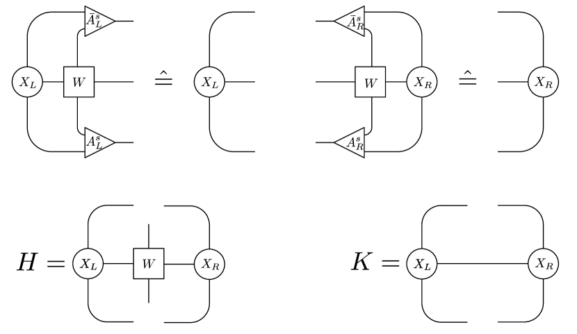
We represent the Hamiltonian (2) in terms of a Matrix Product Operator (MPO) mpo1_supp ; mpo2_supp ; mpo3_supp ; mpolong_supp ; Crosswhite2008 with bond dimension . The projection of onto the MPS tangent plane defines effective Hamiltonians for and for TDVP_Uni_supp . In order to calculate these efficiently it is necessary to determine the left and right (quasi) fixed points of the MPO transfer matrices (c.f. Ref. mpoinf_supp, and Fig. 1)
| (7) |
where a bar denotes complex conjugation and indices (see Fig. 1).
The algorithm in Ref. TDVP_Uni_supp, for a finite chain proceeds by performing the following steps sequentially for each site of the lattice (e.g. in a left-to-right sweep)
-
1.
Calculate as a function of and .
-
2.
Evolve forward in time.
-
3.
Split .
-
4.
Calculate as a function of and .
-
5.
Evolve backward in time and form .
Here refers to tensors updated in previous steps and bold symbols refer to vectorizations of the tensors. Note that both and are calculated from evolved and as-of-yet-unevolved . In the thermodynamic limit, and correspond to the same state and we want to evolve both of them at the same time. The adapted algorithm given in Table 1 achieves this.
The quantities and can be used as a measure of the quality of a time step and of the constraint (4). We reorthonormalize the state according to (5) and (6) if and rise above a certain threshold footnoteA . This new algorithm corresponds to a first-order splitting scheme footnote1_supp with an error scaling of TDVP_Uni_supp .
Notice also, that just as time-dependent density matrix renormalization group (DMRG) tDMRG1_supp ; tDMRG2_supp replaces the effective eigenvalue problem step of ground-state DMRG DMRG1_supp ; DMRG2_supp with a time evolution step, the above scheme replaces the effective eigenvalue problem step of the new ground state algorithm (VUMPS) presented in Ref. VUMPS2017, with a time evolution step.
We increase the bond dimension of the MPS whenever the smallest of the Schmidt values (which are the singular values of ) rises above a certain threshold . For this we use the procedure presented in Appendix B of Ref. VUMPS2017, . In practice we use a time step of , a reorthonormalization threshold of , a bond dimension increase threshold of and a maximum bond dimension of , which – depending on – limits the maximum reachable simulation time severely due to the (at worst) linear increase of entanglement entropy blowS_supp ; Prosen07_supp .
-
1.
Calculate and from current and and form .
-
2.
Evolve forward in time.
-
3.
Evolve forward in time.
-
4.
Determine the optimal updated and by minimizing and under the constraints .
-
5.
(optional) If or rise above some threshold , reorthonormalize the state.
II.3 Loschmidt echo and the return rate
With the definition of the Loschmidt amplitude
| (8) |
the return probability rate function per site
| (9) |
corresponds to (minus) the logarithm of the dominant eigenvalue of the mixed MPS transfer matrix Karrasch13_supp
| (10) |
between MPS tensors at time zero and , whose spectral radius is footnote2_supp . If are the eigenvalues of (10) in descending order by magnitude (i.e. being the largest), then we define the rate-function branches
| (11) |
and the rate function (9) is simply , with all other .
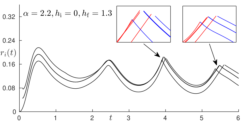
Nonanalyticities of (9) in in the form of cusps arise due to level crossings in the eigenspectrum of (10), which is a feature characteristic of first-order phase transitions. The occurrence of such non-analyticities can thus nicely be anticipated by calculating and following the first few rate-function branches. Cusps arise at branch crossings, where a higher branch becomes the lowest one at some time (see Fig. 2).
The mixed MPS transfer matrix (10) represents an approximation of the true Quantum transfer matrix (QTM) of a real-time path-integral formulation of (8), which can be understood as the result of a renormalization procedure of an effective impurity problem for the true QTM along the real time axis Zauner15_supp ; Rams2015_supp ; Bal2015_supp . Due to this fact, the eigenvalues of the QTM which are reproduced with the highest accuracy are the dominant ones, with smaller and smaller ones being reproduced with less and less accuracy. This also means that the lowest few rate function branches (11) are the most accurate ones with a given finite bond dimension, and the approximation of the return rate function by is valid.
II.4 Alternative calculation of the rate function
Trivially, (8) can also be written as
| (12) |
where in the present case the backward-evolved state can be obtained from the forward-evolved state as , i.e. by complex conjugation. We exploit this fact to evaluate the rate function at time with the MPS at time , i.e. we use the leading eigenvalues of
| (13) |
Thus, can be calculated both from (10) at time and also from (13) at time , and the agreement of both serves as an additional check for the validity of the numerical results. Return rates of the LR-TFIM computed in the framework of iMPS can be found in Ref. Halimeh2016b, .
III Fisher-Zero Lines
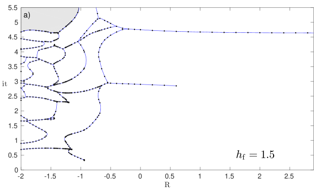
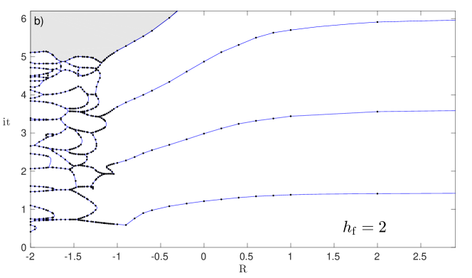
In this section we present additional evidence for the qualitative difference between regular and anomalous cusps by calculating Fisher-zero lines (FZL) in the complex planes for various quenches from for . In particular we show data for a quench to (showing anomalous cusps), and a quench to (showing regular cusps). The plots in Fig. 3 show that the FZL crossing the imaginary axis are also qualitatively different for the two different quenches, which further corroborates that the two types of cusps are distinct.
We consider the boundary partition function
| (14) |
in the complex plane , with . The complex zeros of cause the free energy density analog
| (15) |
to be non-analytic at these points. In the limit of infinite system size these zeros tend to arrange along lines, a fact which was pointed out by Fisher who studied the analytic properties of the thermal partition function of the classical two-dimensional Ising model in the complex temperature plane Fisher1965 . As already discussed, this is similar to the famous Lee-Yang circle theorem Yang1952 ; Lee1952 , which states that the zeros of a classical thermal partition function form circles in the complex fugacity-plane, where is the fugacity, with real and complex and the particle number.
Nonanalyticities in the return rate function therefore appear whenever an FZL crosses the imaginary axis , such that and (14) turns into the Loschmidt amplitude , and equivalently, turns into the return rate function .
Numerically, we can calculate the FZL by utilizing
| (16) |
where we have defined in the last line. To scan the complex plane for non-analyticities of , we therefore prepare the system in state for some fixed (e.g. through imaginary-time evolution) and then perform real-time evolution. A non-analyticity at during this evolution thus implies a Fisher zero at . Note that a similar strategy for calculating FZL in the NN-XXZ model has also been employed in Ref. Andraschko2014, .
In Fig. 3 we show examples for and , with panel (a) for in the anomalous phase where shows anomalous cusps for regular real-time evolution, and panel (b) for in the regular phase, where shows regular cusps. In both cases the Fisher zeros form intricate patterns in the half plane, reminiscent of quenches within the same phase in the NN-TFIM model (cf. e.g. Fig. 1 in Ref. Heyl2013, ) or more complicated quenches in the NN-XXZ model Andraschko2014 .
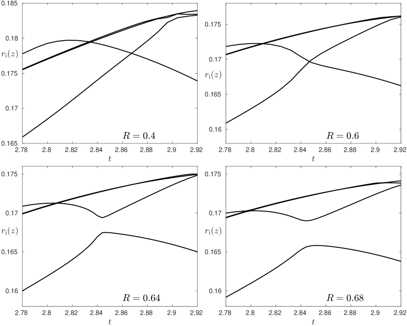
In both cases, a number of FZL emanate from the half plane to cross the imaginary axis and cause cusps in the rate function in the case of pure real-time evolution (). In the regular phase these FZL look very similar to the case of the NN-TFIM, i.e. they continue on to while monotonically increasing (in vs. , see Fig. 3(b)). In contrast, in the anomalous phase, these emanating FZL terminate at some finite (this can be seen in Fig. 3(a) for for the lowest FZL crossing the imaginary axis, which terminates at ). Additionally, the emanating FZL for do not increase monotonically (at least within the considered simulation parameters), which necessarily requires them to terminate at some finite , as there can be no non-analyticities in for footnoteB . Upon decreasing the endpoints of these lines move to smaller and smaller . Whenever such an endpoint crosses the imaginary axis, the corresponding anomalous cusp consequently vanishes in the rate function for real-time evolution. While further decreasing more and more anomalous cusps thus vanish one by one at larger and larger times. This observation is also consistent with Ref. Halimeh2016b, (cf. Fig. 7 therein).
Cusps in the regular phase appear or disappear solely due to individual rate function branches moving relative to one another upon varying . Anomalous cusps on the other hand can also disappear due to branch crossings turning into avoided crossings. Such a scenario is depicted in Fig. 4, which demonstrates how the lowest FZL cutting the imaginary axis in Fig. 3 terminates around .
These additional qualitative differences between FZL in the regular and the anomalous phase further corroborate the existence of two distinct dynamical critical phases for quenches above or below and .
IV Additional anomalous behavior
IV.1 Double cusps
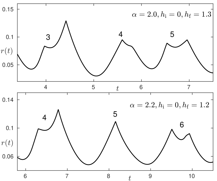
Some of the anomalous cusps that show up for quenches with and develop a double cusp structure in the sense that the tip of these cusps seems to be cut off by another rate-function branch coming down at exactly that time. Examples for such double cusps are shown in Fig. 5. The location of these double cusps also seems to drift with (see also Fig. 7 in Ref. Halimeh2016b, ). The nature and origin of these double cusps remains elusive, although we suspect they could be due to FZL cutting the imaginary axis coming from the half-plane and returning again immediately. As such double cusps do not appear in the regular phase, they constitute another feature distinguishing both phases. It is however worth noting that such double cusps have previously also been observed for the transverse axial next-nearest-neighbor and tilted-field Ising model Karrasch13_supp . We leave the investigation of this double-cusp feature open for future work, as it currently challenges the limits of our numerical capabilities.
IV.2 Crossover between regular and anomalous cusps
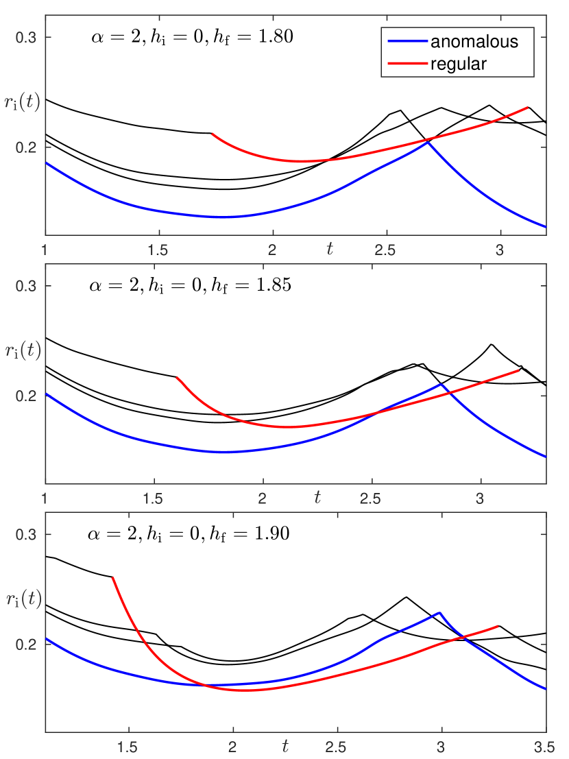
In this section we describe for quenches with and , how regular cusps replace anomalous cusps with approaching and going over . This process is in fact due to a group of rate-function branches (11) that are initially high up for , but come down with increasing , and – after a narrow regime of coexistence around – eventually become lower than the branches responsible for developing anomalous cusps. This new group of rate-function branches then develops regular cusps by crossing one another for all . Such a crossover situation is depicted in Fig. 6 for . Further increasing will cause all anomalous cusps to be completely covered by these new regular branches. The anomalous cusps could in principle still be followed and identified in the now higher-up anomalous rate-function branches, but they no longer contribute to the actual return rate function (which is strictly given by the lowest branch) and cusps therein. Indeed, this provides further evidence of how the anomalous cusps are distinct from their regular counterparts in the sense that they do not simply morph into the regular cusps upon increasing above the dynamical critical point .
V Conclusion
We have presented and discussed in detail how the Loschmidt-echo return rate (and non-analytic cusps therein, related to dynamical phase transitions) for a global quench scenario in the one-dimensional long-range (power-law interacting) transverse-field Ising model can be efficiently calculated in the framework of infinite Matrix Product States. We demonstrate in particular, that – in contrast to finite-size approaches – working directly in the thermodynamic limit enables an unambiguous identification of non-analyticities, which arise from level crossings in the eigenvalues of the Matrix Product State transfer matrix. We have further illustrated how the anomalous and regular dynamical critical phases, first reported in Ref. Halimeh2016b, , are distinct by showing that they arise due to qualitatively different Fisher-zero-line behavior. Whereas the regular phase constitutes cusps that arise due to the relative movement of so-called rate function branches of the Matrix Product State transfer matrix, the anomalous cusps are related to avoided crossings of these branches turning into actual crossings. Moreover, we have presented results showing double-cusp properties that further set the anomalous phase apart from its regular counterpart. Even though we cannot ascertain the origin of these double cusps, we do hypothesize that they arise due to Fisher-zero lines cutting the imaginary axis and then quickly turning around and cutting it again. Our work further validates the existence of the anomalous phase in the one-dimensional transverse-field Ising model for quenches from the -symmetry-broken equilibrium phase to a final value of the transverse field below the dynamical critical point. Moreover, the method discussed in this work provides a versatile tool that is suitable to investigate, naturally in the thermodynamic limit, dynamical phase transitions in the context of non-analyticities in the Loschmidt-echo return rate, and properly characterize its different phases in various models, even though here we only tackle the transverse-field Ising chain with power-law interactions.
Acknowledgments
We thank Damian Draxler, Jutho Haegeman, Frank Verstraete, Ian P. McCulloch, and Johannes Lang for inspiring and helpful discussions. V. Z.-S. gratefully acknowledges support from the Austrian Science Fund (FWF): F4104 SFB ViCoM and F4014 SFB FoQuS. The computational results presented have been achieved in part using the Vienna Scientific Cluster (VSC).
References
- (1) J. Cardy, Scaling and Renormalization in Statistical Physics (Cambridge University Press, 1996).
- (2) S. Sachdev, Quantum Phase Transitions (Cambridge University Press, 1999).
- (3) M. Fisher, Rev. Mod. Phys. 46, 597 (1974).
- (4) M. Heyl, A. Polkovnikov, and S. Kehrein, Phys. Rev. Lett. 110, 135704 (2013).
- (5) M. Heyl, Phys. Rev. Lett. 115, 140602 (2015).
- (6) J. C. Halimeh and V. Zauner-Stauber, arXiv:1610:02019.
- (7) B. Zunkovic, A. Silva, and M. Fabrizio, Phil. Trans. R. Soc. A 374, 20150160 (2016).
- (8) B. Zunkovic, M. Heyl, M. Knap, and A. Silva, arxiv:1609.08482.
- (9) I. Homrighausen, N. O. Abeling, V. Zauner-Stauber, and J. C. Halimeh, arXiv:1703:09195.
- (10) C. N. Yang and T. D. Lee, Phys. Rev. 87, 404 (1952).
- (11) T. D. Lee and C. N. Yang, Phys. Rev. 87, 410 (1952).
- (12) P. J. Kortman and R. B. Griffiths, Phys. Rev. Lett. 27, 1439 (1971).
- (13) M. E. Fisher, Phys. Rev. Lett. 40, 1610 (1978).
- (14) M. E. Fisher, Statistical Physics, Weak Interactions, Field Theory, Lectures in Theoretical Physics Vol. VII C (University of Colorado Press, Boulder, 1965).
- (15) F. Andraschko and J. Sirker, Phys. Rev. B 89, 125120 (2014).
- (16) S. Vajna and B. Dóra, Phys. Rev. B 89, 161105(R) (2014).
- (17) G. Vidal, Phys. Rev. Lett. 93, 040502 (2004).
- (18) A. J. Daley, C. Kollath, U. Schollwöck, and G. Vidal, J. Stat. Mech.: Theor. Exp. P04005 (2004).
- (19) S.R. White and A.E. Feiguin, Phys. Rev. Lett. 93, 076401 (2004).
- (20) S.R. White, Phys. Rev. Lett. 69, 2863 (1992).
- (21) S.R. White, Phys. Rev. B 48, 10345 (1993).
- (22) M. Fannes, B. Nachtergaele, and R. Werner, Comm. Math. Phys. 144, 443 (1992).
- (23) F. Verstraete and V. Murg, J. I. Cirac, Adv. Phys. 57, 143 (2008).
- (24) U. Schollwöck, Ann. Phys. (NY) 326, 96 (2011).
- (25) G. Vidal, Phys. Rev. Lett. 98, 070201 (2007).
- (26) H. F. Trotter, Proc. Am. Math. Soc. 10, 545 (1959).
- (27) M. Suzuki, Prog. Theor. Phys. 56, 1454 (1976).
- (28) M. P. Zaletel, R. S. K. Mong, C. Karrasch, J. E. Moore, and F. Pollmann, Phys. Rev. B 91, 165112 (2015).
- (29) J. Haegeman, T. J. Osborne, and F. Verstraete, Phys. Rev. B 88, 075133 (2013).
- (30) J. Haegeman et al., Phys. Rev. Lett. 107, 070601 (2011).
- (31) J. Haegeman et al., Phys. Rev. B 94, 165116 (2016).
- (32) G. M. Crosswhite, A. C. Doherty, and G. Vidal, Phys. Rev. B 78, 035116 (2008).
- (33) F. Verstraete, J. J. Garcia-Ripoll, and J. I. Cirac, Phys. Rev. Lett. 93, 207204 (2004).
- (34) I. P. McCulloch, J. Stat. Mech.: Theor. Exp. (2007) P10014.
- (35) B. Pirvu, V. Murg, J. I. Cirac, and F. Verstraete, New J. Phys. 12, 025012 (2010).
- (36) G. M. Crosswhite and D. Bacon, Phys. Rev. A 78, 012356 (2008); F. Fröwis, V. Nebendahl, and W. Dür, Phys. Rev. A 81, 062337 (2010).
- (37) L. Michel and I.P. McCulloch, arXiv:1008.4667 (2010).
- (38) For an inverse-free method of reorthonormalizing an iMPS, see e.g. Ref. MPO_review_supp, .
- (39) J. Haegeman, F. Verstraete, Ann. Rev. Cond. Mat. Phys. 8, 355 (2017).
- (40) Higher order schemes can be constructed in a slightly different way, but are computationally much more unfavorable than performing a first order step several times for a smaller time step.
- (41) V. Zauner-Stauber, L. Vanderstraeten, M.T. Fishman, F. Verstraete, and J. Haegeman, arXiv:1701.07035.
- (42) N. Schuch, M. M. Wolf, K. G. H. Vollbrecht, and J. I. Cirac, New J. Phys. 10, 033032 (2008).
- (43) T. Prosen and M. Znidaric, Phys. Rev. E 75, 015202 (2007).
- (44) C. Karrasch and D. Schuricht, Phys. Rev. B 87, 195104 (2013).
- (45) The gauge choices for and do not affect the eigenvalues of and are therefore irrelevant.
- (46) V. Zauner et al., New J. Phys. 17, 053002 (2015).
- (47) M. M. Rams, V. Zauner, M. Bal, J. Haegeman, and F. Verstraete, Phys. Rev. B 92, 235150 (2015).
- (48) M. Bal, M. M. Rams, V. Zauner, J. Haegeman, and F. Verstraete, Phys. Rev. B 94, 205122 (2016).
- (49) For the initial state is the ground state of the evolution Hamiltonian and therefore a stationary state of the evolution.