Efficient simulation of Brown-Resnick processes
based on variance reduction of Gaussian processes

Abstract

  
Brown-Resnick processes are max-stable processes that are associated to Gaussian processes. Their simulation is often based on the corresponding spectral representation which is not unique. We study to what extent simulation accuracy and efficiency can be improved by minimizing the maximal variance of the underlying Gaussian process. Such a minimization is a difficult mathematical problem that also depends on the geometry of the simulation domain. We extend Matheron’s (1974) seminal contribution in two aspects: (i) making his description of a minimal maximal variance explicit for convex variograms on symmetric domains and (ii) proving that the same strategy reduces the maximal variance also for a huge class of non-convex variograms representable through a Bernstein function. A simulation study confirms that our non-costly modification can lead to substantial improvements among Gaussian representations. We also compare it with three other established algorithms.

Keywords: Brown-Resnick process, Gaussian process, max-stable process, simulation, spatial extremes, variance reduction, variogram
2010 MSC: Primary 60G70; 60G15
2010 MSC: Secondary 60G60

1 Introduction

Many powerful tools in geostatistics are conveniently based on Gaussian processes as an underlying probabilistic model for uncertainty (Chilès and Delfiner, 2012; Gelfand et al., 2010). By contrast, assessing the extreme values of spatial data genuinely requires statistical methodology that goes beyond such tools. A common approach from extreme value analysis is the usage of max-stable models instead. In particular, the class of Brown-Resnick processes (Brown and Resnick, 1977; Kabluchko et al., 2009) has emerged as a now widely adopted class of processes considered in the analysis of spatial data, cf. e.g. Asadi et al. (2015); Buhl and Klüppelberg (2016); Davison et al. (2013); Einmahl et al. (2016); Engelke et al. (2015); Gaume et al. (2013); Oesting et al. (2017); Sang and Genton (2014); Oesting and Stein (2017); Thibaud et al. (2016).

There is a strong connection between Brown-Resnick processes and Gaussian processes: First, Brown-Resnick processes arise as the only possible non-degenerate limits of maxima of appropriately rescaled independent Gaussian processes (Kabluchko et al., 2009; Kabluchko, 2011). Second, they can be represented as maxima of a convolution of the points of a Poisson point process and Gaussian processes. As the number of Gaussian processes involved in the maximum is locally finite, Brown-Resnick processes still inherit various properties from Gaussian processes on a local level. They are parsimonious models in the sense that their law is fully specified by a bivariate quantity, namely the variogram of the underlying Gaussian process. On the other hand, they are still very flexible in the sense that various features such as smoothness, scale or nugget effect can be controlled by the choice of variogram family. All of this makes Brown-Resnick processes popular consistent spatial models and marks their status as a benchmark in spatial extremes.

To extract probabilistic properties of interest from a fitted Brown-Resnick model, it is usually necessary to be able to efficiently simulate from the fitted model. Meanwhile, several approaches for this task have been developed. Starting from the basic threshold stopping approach based on the work of Schlather (2002) using plainly the original definition of a Brown-Resnick process, Oesting et al. (2012), Dieker and Mikosch (2015) and Oesting et al. (2018) achieved further improvements that are based on modified spectral representations. Based on different techniques, Dombry et al. (2016) and Liu et al. (2016) proposed the extremal functions and the record-breakers approach, respectively, both of which together with the normalization method of Oesting et al. (2018) can now be seen as state-of-the-art algorithms for the exact simulation of Brown-Resnick processes.

When dealing with spatial data, the study area on which the process should be simulated may be large with respect to its spatial extent or the number of locations therein. In such situations, exact simulation of Brown-Resnick processes via one of the state-of-art algorithms can be very time-consuming and depending on the purpose of the application it can be more appropriate to admit (desirably small) simulation errors. Once a trade-off between accuracy and efficiency is necessary, it is no longer clear which of the previously considered simulation approaches performs “best”. Keeping this in mind, we return to the initial threshold stopping approach devised by Schlather (2002) from a new perspective in this work. We explore to what extent a modified choice of Gaussian spectral representation of Brown-Resnick processes can improve the efficiency or accuracy of the simulation and whether an improved threshold stopping approach can compete with state-of-the-art simulation when an error is admitted. Dealing with these questions ultimately leads us to a classical minimization problem for Gaussian processes, namely, to find a Gaussian process whose maximal variance across the simulation domain is minimized, while its variogram on this domain is fixed. In this regard, we extent Matheron’s (1974) seminal contribution in two aspects: (i) making his description of a minimal maximal variance explicit for convex variograms on symmetric domains and (ii) proving that the same strategy reduces the maximal variance also for the huge class of non-convex variograms that can be represented via Bernstein functions.

The manuscript is organized as follows. Section 2 recalls the spectral representation of Brown-Resnick processes and revisits Schlather’s threshold stopping algorithm for the simulation of max-stable processes on a compact domain. We explain why it is beneficial for the underlying Gaussian process to have a reduced maximal variance across the simulation domain. Subsequently, Section 3, the main contribution, provides two results complementing Matheron (1974) for the corresponding minimization problem and elaborates on discretization effects. Throughout the text, the most popular family of Brown-Resnick processes that are associated to fractional Brownian sheets, figure as an example. In Section 4 we report the setup and results of a simulation study for this family of models, where we also compare our approach with three other methods. Finally, we end with a discussion of our findings in Section 5. Proofs and additional auxiliary results are deferred to Appendix A.

2 Spectral representations and threshold stopping

Let $Z=\{Z(\bm{x})\}_{\bm{x}\in\mathbb{R}^{d}}$ be a simple max-stable process on $\mathbb{R}^{d}$, which means that for each $n\in\mathbb{N}$ and $n$ i.i.d. copies $Z_{1},\dots,Z_{n}$ of $Z$, the process $Z_{1}\vee\dots\vee Z_{n}$ of the pointwise maxima has the same law as $nZ$ and that $Z$ has standard Fréchet margins: $\mathbb{P}(Z(\bm{x})\leq z)=\exp(-1/z)$ for $z>0$, $\bm{x}\in\mathbb{R}^{d}$. It was shown by de Haan (1984) that, if $Z$ is continuous in probability, there exists a non-negative stochastic process $V=\{V(\bm{x})\}_{\bm{x}\in\mathbb{R}^{d}}$ on $\mathbb{R}^{d}$ with $\mathbb{E}(V(\bm{x}))=1$, $\bm{x}\in\mathbb{R}^{d}$, such that the law of the simple max-stable process $Z$ is recovered from the following max-series

$$\{Z(\bm{x})\}_{\bm{x}\in\mathbb{R}^{d}}\stackrel{{\scriptstyle\mathcal{D}}}{{=}}\bigg{\{}\bigvee_{k=1}^{\infty}U_{k}V_{k}(\bm{x})\bigg{\}}_{\bm{x}\in\mathbb{R}^{d}}.$$ (1)

Here $\{U_{k}\}_{k=1}^{\infty}$ denotes a Poisson point process on $(0,\infty)$ with intensity measure $u^{-2}\mathrm{d}u$, which is independent of the i.i.d. sequence $\{V_{k}\}_{k=1}^{\infty}$ of copies of $V$. The process $V$ is often called spectral process and the representation (1) referred to as spectral representation of $Z$. By Giné et al. (1990), if $Z$ has continuous sample paths, the trajectories of $V$ will also be continuous and vice versa, such that the sequence $\{(U_{k},V_{k})\}_{k=1}^{\infty}$ may be considered as an independently marked Poisson process $\Pi$ on $(0,\infty)\times C(\mathbb{R}^{d})$ with intensity measure

$$\Lambda((u,\infty)\times A)=u^{-1}\mathbb{P}(V\in A),\quad u>0,\ A\subset C(\mathbb{R}^{d})\ \text{Borel},$$

where $C(\mathbb{R}^{d})$ is endowed with the usual topology of uniform convergence on compact subsets.

One popular choice for the spectral process $V$ of a max-stable process $Z$ is a log-Gaussian process of the form

$$V(\bm{x})=e^{\eta(\bm{x})}\quad\text{with}\quad\eta(\bm{x})=W(\bm{x})-\frac{\mathrm{Var}(W(\bm{x}))}{2},\quad\bm{x}\in\mathbb{R}^{d},$$ (2)

where $W$ is a zero-mean Gaussian process $W$ with stationary increments. The associated max-stable process $Z$, called Brown-Resnick process, was introduced and many of its properties were analysed in Kabluchko et al. (2009). The requirement that $W$ has stationary increments means that the law of the process $\{W(\bm{x}+\bm{h})-W(\bm{x})\}_{\bm{h}\in\mathbb{R}^{d}}$ does not depend on $\bm{x}\in\mathbb{R}^{d}$. Since $W$ is zero-mean Gaussian, it is equivalent to the intrinsic stationarity of the process $W$, that is, the stationarity of the process $\{W(\bm{x}+\bm{h})-W(\bm{x})\}_{\bm{x}\in\mathbb{R}^{d}}$ for all $\bm{h}\in\mathbb{R}^{d}$, cf. e.g. page 108 in Strokorb (2013). It ensures that the resulting max-stable process $Z$ is stationary and its law is uniquely specified by the variogram

$$\gamma(\bm{x}-\bm{y})=\mathbb{E}(W(\bm{x})-W(\bm{y}))^{2},\quad\bm{x},\bm{y}\in\mathbb{R}^{d}.$$

Gneiting et al. (2001) show that a function $\gamma:\mathbb{R}^{d}\rightarrow\mathbb{R}$ is a (not necessarily centered) variogram of an intrinsically stationary Gaussian random field $W$ if and only if $\gamma(\bm{0})=0$ and $\gamma$ is negative definite in the sense that $\gamma(-\bm{x})=\gamma(\bm{x})$ for $\bm{x}\in\mathbb{R}^{d}$ and

$$\sum_{i=1}^{n}\sum_{j=1}^{n}a_{i}\gamma(\bm{x}_{i}-\bm{x}_{j})a_{j}\leq 0$$ (3)

for all finite systems $\bm{x}_{1},\dots,\bm{x}_{n}\in\mathbb{R}^{d}$ and $a_{1},\dots,a_{n}\in\mathbb{R}$ with $a_{1}+\dots+a_{n}=0$. The most popular family of variograms used in practice is $\gamma(\bm{h})=\lVert\bm{h}/s\rVert^{\alpha}$ for some $\alpha\in(0,2]$ and $s>0$ corresponding to fractional Brownian sheets. This family of variograms will also serve as an illustrating example throughout this text. It can be shown that all fractional Brownian sheets admit continuous trajectories (cf. Thm. 1.4.1. in Adler and Taylor, 2009, for instance). Hence, the resulting max-stable process is also continuous.

Henceforth, we will restrict our attention to a compact subset $K\subset\mathbb{R}^{d}$. Let $\{E_{i}\}_{i=1}^{\infty}$ and $\{V_{k}\}_{k=1}^{\infty}$ be two independent i.i.d. sequences of standard exponential random variables and copies of $V$, respectively, and set $U_{k}=(\sum_{i=1}^{k}E_{i})^{-1}$, $k=1,2,\dots$. As the points $\{(U_{k},V_{k})\}_{k=1}^{\infty}$ form a Poisson point process with intensity measure $\Lambda$, the finite approximations

$$Z^{(n)}(\bm{x})=\bigvee_{k=1}^{n}U_{k}V_{k}(\bm{x}),\quad\bm{x}\in K,$$

almost surely converge to a limit process $Z^{(\infty)}$ (as $n\to\infty$) satisfying $Z^{(\infty)}\stackrel{{\scriptstyle\mathcal{D}}}{{=}}Z$. To obtain an approximation built from a finite number of exponential random variables $E_{k}$ and stochastic processes $V_{k}$, often the process $Z^{(T)}$ is considered where $T$ is a stopping time defined as

$$T=T_{K,\tau}=\min\Big{\{}k\geq 1:U_{k+1}\tau\leq\inf_{\bm{x}\in K}Z^{(k)}(\bm{x})\Big{\}}$$ (4)

for some $\tau>0$. Such an approximation $Z^{(T)}$ yields an exact simulation of a general max-stable process $Z$, i.e. $Z^{(T)}=Z^{(\infty)}$ a.s., if the condition $\sup_{\bm{x}\in K}V(\bm{x})<\tau$ is a.s. satisfied and for such situations this approach has been proposed in Schlather (2002). In the case when $V$ is log-Gaussian, however, as in (2), an approximation error may occur. The probability that such an error occurs is given by

$${}\mathcal{P}_{K,\tau}={} \mathbb{P}(Z^{(T)}\neq Z^{(\infty)}\text{ on }K)$$

$$={} 1-\mathbb{E}_{Z^{(T)}}\bigg{\{}\exp\bigg{(}-\mathbb{E}_{V}\bigg{(}\sup_{\bm{x}\in K}\frac{V(\bm{x})}{Z^{(T)}(\bm{x})}-\sup_{\bm{x}\in K}\frac{\tau}{Z^{(T)}(\bm{x})}\bigg{)}_{+}\bigg{)}\bigg{\}}$$ (5)

(Oesting and Strokorb, 2018), where the symbol $\mathbb{E}$ with a stochastic process as a subscript means that the expectation is meant with respect to this process.

The situation is particulary difficult, when the spectral functions’ variance $\mathrm{Var}(V(\bm{x}))$ is large, since trajectories $U_{k}V_{k}(\bm{x})$ that are generated late in a hypothetical unstopped simulation can have an outsize influence on the sample path, i.e. stopping too soon has profound consequences on the quality of the output. Specifically, for Brown-Resnick processes, the variance $\mathrm{Var}(V(\bm{x}))$ of the log-Gaussian spectral functions in (2) is of order $\exp({\mathrm{Var}(W(\bm{x}))})$ and this order can be excessive depending on the values of $\mathrm{Var}(W(\bm{x}))$ on the simulation domain $K$. For instance, if $W$ is the standard (“original”) fractional Brownian sheet that vanishes at the origin $\bm{0}\in\mathbb{R}^{d}$ (i.e. $W(\bm{0})=0$ a.s.), the variance $\mathrm{Var}(V(\bm{x}))$ is exponential in $\lVert\bm{x}\rVert^{\alpha}$. This poses a major challenge for stopping-time based approximate simulation.

What might however mitigate this challenge to some extent is the fact that there is still some choice among the log-Gaussian representations of Brown-Resnick processes. While the variogram $\gamma$ uniquely determines the law of the associated Brown-Resnick process $Z$, it does not uniquely determine the law of the Gaussian process $W$ in its spectral representation (2). Various covariance functions $C(\bm{x},\bm{y})=\mathrm{Cov}(W(\bm{x}),W(\bm{y}))$ on $K$ share the same variogram

$$\gamma(\bm{x}-\bm{y})=C(\bm{x},\bm{x})-2C(\bm{x},\bm{y})+C(\bm{y},\bm{y}),\quad\bm{x},\bm{y}\in K.$$

In what follows, we seek to find such Gaussian representations $W$ for a prescribed variogram $\gamma$, whose variances $\mathrm{Var}(V(\bm{x}))$ are uniformly small over the simulation domain $K$. More precisely, we address the following problem in Section 3 and study the consequences of using low-variance Gaussian representations in the threshold stopping procedure in Section 4.

Problem 1.

Let $\mathcal{W}_{K}(\gamma)$ be the set of Gaussian processes with variogram $\gamma$ on the compact simulation window $K$. If it exists, identify a Gaussian process $W_{\min}\in\mathcal{W}_{K}(\gamma)$ that minimizes the functional

$$W\mapsto\sup_{\bm{x}\in K}\mathrm{Var}(W(\bm{x})).$$

Remark 2.1.

Addressing Problem 1 will also be beneficial for reducing the error probability $\mathcal{P}_{K,\tau}$ in (5) for high thresholds $\tau$ or several other error terms in Oesting and Strokorb (2018). To see this, note that Proposition A.1 in the Appendix A ensures that, for each positive $z\in C(K)$, the tail probabilities

$$\mathbb{P}\bigg{(}\sup_{\bm{x}\in K}\frac{V(\bm{x})}{{z(\bm{x})}}>u\bigg{)}=\mathbb{P}\bigg{(}\sup_{\bm{x}\in K}\exp\bigg{\{}W(\bm{x})-\frac{\mathrm{Var}(W(\bm{x}))}{2}-\log z(\bm{x})\bigg{\}}>u\bigg{)}$$

decay as fast as possible as $u\uparrow\infty$ if $V$ is built from the solution of Problem 1. This property entails that

$$\mathbb{E}\bigg{(}\sup_{\bm{x}\in K}\frac{V(\bm{x})}{{z(\bm{x})}}-\sup_{\bm{x}\in K}\frac{\tau}{{z(\bm{x})}}\bigg{)}_{+}=\int_{\tau\,\sup_{\bm{x}\in K}{{1/z(\bm{x})}}}^{\infty}\mathbb{P}\bigg{(}\sup_{\bm{x}\in K}\frac{V(\bm{x})}{{z(\bm{x})}}>u\bigg{)}\,\mathrm{d}u$$

becomes smaller for each positive function $z\in C(K)$ and for high thresholds $\tau>0$.

3 Minimal log-Gaussian representations

To the best of our knowledge, Problem 1 has first been addressed by Matheron (1974) who introduced the notion of the minimal representation of an intrinsically stationary process. Starting from the fact that – given a specific centered Gaussian process $W_{0}$ on $K$ with variogram $\gamma$ – any other centered Gaussian process $W$ on $K$ with the same variogram is of the form $W(\bm{x})=W_{0}(\bm{x})+B$ for some square-integrable random variable $B$, he defined the minimal representation of $W_{0}$ as the process $W_{\min}(\bm{x})=W_{0}(\bm{x})+B_{\min}$ such that

$$\sup_{\bm{x}\in K}\mathrm{Var}(W_{\min}(\bm{x}))=\inf_{B\in L^{2}(\Omega,\mathcal{A},\mathbb{P})}\sup_{\bm{x}\in K}\mathrm{Var}(W_{0}(\bm{x})+B),$$

i.e. the process whose covariance function $C_{\min}$ is the solution of Problem 1. Matheron (1974) further showed that, for any sample-continuous intrinsically stationary Gaussian process, a unique minimal representation exists and has the form

$$W_{\min}(\bm{x})=W_{0}(\bm{x})-\int_{K}W_{0}(\tilde{\bm{x}})\,\lambda_{\min}(\mathrm{d}\tilde{\bm{x}}),\quad\bm{x}\in K,$$ (6)

for some probability measure $\lambda_{\min}$ on $K$. The resulting covariance function $C_{\min}$ on $K\times K$ can be obtained from

$$2C_{\min}(\bm{x},\bm{y})=-\gamma(\bm{x}-\bm{y}) +\int_{K}\gamma(\bm{x}-\tilde{\bm{x}})\,\lambda_{\min}(\mathrm{d}\tilde{\bm{x}})$$

$$+\int_{K}\gamma(\bm{y}-\tilde{\bm{y}})\,\lambda_{\min}(\mathrm{d}\tilde{\bm{y}})-\int_{K}\int_{K}\gamma(\tilde{\bm{x}}-\tilde{\bm{y}})\,\lambda_{\min}(\mathrm{d}\tilde{\bm{x}})\,\lambda_{\min}(\mathrm{d}\tilde{\bm{y}}).$$ (7)

Note that the covariance and, consequently, the law of the minimal representation does not depend on the initially chosen random field $W_{0}$.

3.1 Minimal solution for convex variograms

If the variogram $\gamma$ is convex and regular in the sense that for two probability measures $\lambda$ and $\mu$ on the compact domain $K$ the equality

$$\int_{K}\int_{K}\gamma(\bm{x}-\bm{y})(\lambda-\mu)(\mathrm{d}\bm{x})(\lambda-\mu)(\mathrm{d}\bm{y})=0$$

implies $\lambda=\mu$, then Matheron (1974) characterizes the minimizing probability measure $\lambda_{\min}$ by the following two properties

$$\text{Supp}(\lambda_{\min}) \subset\text{Ex}(K),$$ (8)

$$\int_{K}\gamma(\bm{x}-\tilde{\bm{y}})\,\lambda_{\min}(\mathrm{d}\tilde{\bm{y}}) \leq\int_{K}\int_{K}\gamma(\tilde{\bm{x}}-\tilde{\bm{y}})\,\lambda_{\min}(\mathrm{d}\tilde{\bm{x}})\,\lambda_{\min}(\mathrm{d}\tilde{\bm{y}})\quad\text{ for all }\bm{x}\in\text{Ex}(K).$$ (9)

Here, $\text{Ex}(K)$ denotes the set of extremal points of $K$, i.e. the elements of $K$ that cannot be decomposed non-trivially as a convex combination of any two other points of $K$. For instance, the $2^{d}$ vertices $(\pm R_{1},\pm R_{2},\dots,\pm R_{d})$ of a $d$-dimensional hyperrectangle $K=\prod_{i=1}^{d}[-R_{i},R_{i}]$ form its extremal points. In fact, hyperrectangles are the most natural simulation domains that we consider in practice and we will be mainly interested in this case. For a hyperrectangle $K=\prod_{i=1}^{d}[-R_{i},R_{i}]$ it is also often convenient to label its vertex set $\text{Ex}(K)$ by subsets $A$ of $\{1,\dots,d\}$ through

$$\text{Ex}\Big{(}\prod_{i=1}^{d}[-R_{i},R_{i}]\Big{)}=\{\bm{v}_{A}\,:\,A\subset\{1,\dots,d\}\},\quad\bm{v}_{A}=(\sigma^{A}_{i}R_{i})_{i=1}^{d},\quad\sigma^{A}_{i}=\begin{cases}+1&i\in A\\ -1&i\not\in A\end{cases}.$$ (10)

When the variogram $\gamma$ and the simulation domain $K$ are sufficiently symmetric, the measure $\lambda_{\min}$ can be made even more explicit. To this end, we refer to the set of orthogonal transformations $\bm{M}\in O(\mathbb{R}^{d})$, such that $\bm{M}A=\{\bm{M}\bm{a}\,:\,\bm{a}\in A\}$ coincides with $A$, as the symmetry group $\text{Sym}(A)$ of a set $A\subset\mathbb{R}^{d}$.

Proposition 3.1.

Let $W_{0}$ be a sample-continuous intrinsically stationary Gaussian process on $\mathbb{R}^{d}$ with convex variogram $\gamma(\bm{h})=\psi(\lVert\bm{h}\rVert^{2})$, $\bm{h}\in\mathbb{R}^{d}$. Let $K\subset\mathbb{R}^{d}$ be a compact domain, whose symmetry group ${\text{Sym}}({\text{Ex}}(K))$ acts transitively on the set of extremal points ${\text{Ex}}(K)$. Then the minimizing measure $\lambda_{\min}$ in the sense of (6) is the uniform distribution on ${\text{Ex}}(K)$.

Example 3.2.

Let $W_{0}$ be a fractional Brownian sheet on $\mathbb{R}^{d}$ with variogram $\gamma(\bm{h})=\lVert\bm{h}/s\rVert^{\alpha}$ for some $\alpha\in[1,2)$, $s>0$. Let $K=\prod_{i=1}^{d}[-R_{i},R_{i}]$ be a $d$-dimensional hyperrectangle, whose vertices $\bm{v}_{A}$ are labelled by subsets $A\subset\{1,\dots,d\}$ as in (10). Then Proposition 3.1 applies and says that the process

$$W(\bm{x})=W_{0}(\bm{x})-\frac{1}{2^{d}}\sum_{A\subset\{1,\dots,d\}}W_{0}(\bm{v}_{A}),\quad\bm{x}\in K,$$ (11)

possesses the smallest maximal variance on $K$ among the family of intrinsically stationary Gaussian processes with variogram $\gamma$.

Remark 3.3.

Matheron (1974) provides the argument for (8) and (9) being necessary and sufficient for $\lambda_{\min}$ to be the minimal measure for compact and convex sets $K$. It is however easily checked that convexity of $K$ can be dispensed with.

3.2 Reduction of maximal variance for non-convex variograms

For non-convex variograms it is not so clear how to obtain the minimizing measure $\lambda_{\min}$ explicitly, not even for hyperrectangles. However, in many situations it is still possible to apply the same strategy as in Example 3.2 to substantially reduce the maximal variance. At least we show below that this is possible when the variogram $\gamma$ can be represented as $\gamma(\bm{h})=\psi(\lVert\bm{h}\rVert^{2})$, $\bm{h}\in\mathbb{R}^{d}$, for a Bernstein function $\psi$.

There are several definitions of Bernstein functions and various properties and examples have been summarized in the recent monograph Schilling et al. (2010). For us it will be convenient to define a Bernstein function as a function $\psi:\mathbb{R}_{+}\rightarrow\mathbb{R}$ on the positive real line $\mathbb{R}_{+}=[0,\infty)$ that is bounded from below and negative definite in the sense that

$$\sum_{i=1}^{n}\sum_{j=1}^{n}a_{i}\psi(s_{i}+s_{j})a_{j}\leq 0$$ (12)

for all finite systems $s_{1},\dots,s_{n}\in\mathbb{R}_{+}$ and $a_{1},\dots,a_{n}\in\mathbb{R}$ with $a_{1}+\dots+a_{n}=0$, cf. page 113/114 of Berg et al. (1984). Note that we deviate from most of the literature where continuity at $0$ is additionally required. The following lemma shows that considering only variograms that can be represented by Bernstein functions is not a serious restriction and, secondly, that Bernstein functions obey certain monotonicity properties defined as follows: A function $f:\mathbb{R}_{+}\rightarrow\mathbb{R}$ is $n$-alternating if it satisfies

$$\Delta_{s_{1}}\Delta_{s_{2}}\dots\Delta_{s_{n}}f(s)=\sum_{A\subset\{1,\dots,n\}}(-1)^{\lvert A\rvert}f\bigg{(}s+\sum_{i\in A}s_{i}\bigg{)}\leq 0$$ (13)

for $s,s_{1},s_{2},\dots,s_{n}\in\mathbb{R}_{+}$. In particular, $f$ is $1$-alternating if and only if it is non-decreasing.

Lemma 3.4.

Let $\psi:\mathbb{R}_{+}\rightarrow\mathbb{R}$ be bounded from below. Then the following statements are equivalent.

1. $\psi$ is a Bernstein function.

2. $\psi(\lVert\bm{h}\rVert^{2})$, $\bm{h}\in\mathbb{R}^{d}$, is negative definite in the sense of (3) for any dimension $d\in\mathbb{N}$.

3. $\psi$ is $n$-alternating of any order $n\in\mathbb{N}$.

In particular, the equivalence of (i) and (ii) means that $\psi$ is a Bernstein function if and only if $\gamma(\bm{h})=\psi(\lVert\bm{h}\rVert^{2})$, $\bm{h}\in\mathbb{R}^{d}$, is a valid (not necessarily centred) variogram in any dimension $d\in\mathbb{N}$. Finally, this allows us to transfer the strategy from Example 3.2 to non-convex variograms as follows.

Proposition 3.5.

Let $W_{0}$ be an intrinsically stationary Gaussian process on $\mathbb{R}^{d}$ with variogram $\gamma(\bm{h})=\psi(\lVert\bm{h}\rVert^{2})$, $\bm{h}\in\mathbb{R}^{d}$, for a Bernstein function $\psi$, and $W_{0}(\bm{0})=0$ almost surely. Let $K=\prod_{i=1}^{d}[-R_{i},R_{i}]$ be a $d$-dimensional hyperrectangle, whose vertices $\bm{v}_{A}$ are labelled by subsets $A\subset\{1,\dots,d\}$ as in (10). Then the maximal variance of the modified process $W$ in (11) is at least as small as the maximal variance of the original process $W_{0}$ on the domain $K$, i.e.

$$\sup_{\bm{x}\in K}\mathrm{Var}(W(\bm{x}))\leq\sup_{\bm{x}\in K}\mathrm{Var}(W_{0}(\bm{x})).$$

Example 3.6.

Proposition 3.5 applies to the situation of Example 3.2 with $\alpha\in[1,2)$ replaced by arbitrary $\alpha\in(0,2)$ and $W_{0}(\bm{0})=0$ almost surely. In particular, the maximal variance on the hyperrectangle $K$ can also be reduced for $\alpha\in(0,1)$ by the same simple trick of subtracting the vertices of $K$ with equal weights that we applied already for $\alpha\in[1,2)$ in Example 3.2. Summarizing, we see that this trick reduces the maximal variance on $K$ for any fractional Brownian sheet. For $\alpha\in[1,2)$ it even minimizes this maximal variance, cf. Example 3.2.

Remark 3.7.

1. In fact, the proof of Proposition 3.5 only requires $n$-alternation of $\psi$ for $n\leq 3$ and not necessarily that $\psi$ is a Bernstein function.

2. In Examples 3.2, 3.6 and Proposition 3.5 the variogram $\gamma(\bm{h})$ can be replaced by $\tilde{\gamma}(\bm{h})=\gamma(\bm{M}\bm{h})$, where $\bm{M}$ is any invertible symmetric $d\times d$ matrix. This is possible, since such a transformation of $\mathbb{R}^{d}$ maps hyperrectangles that are centered at the origin again into hyperrectangles that are centered at the origin, whence Propositions 3.1 and 3.5 can be applied to the transformed processes $W_{0}(\bm{M}^{-1}\bm{x})$, $W(\bm{M}^{-1}\bm{x})$, $\bm{x}\in\mathbb{R}^{d}$, and their variogram $\tilde{\gamma}(\bm{M}^{-1}\bm{h})=\gamma(\bm{h})$, $\bm{h}\in\mathbb{R}^{d}$.

3.3 Minimal $K$-stationary representations

There are some situations, in which we can even compare the improvements of the variance reduction of Proposition 3.5 to the true minimal maximal variance on the simulation domain $K$. This is the case when the minimizing measure $\lambda_{\min}$ leads to a $K$-stationary solution, that is, when $C_{\min}(\bm{x},\bm{y})$ in (7) only depends on $\bm{x}-\bm{y}$ for $\bm{x},\bm{y}\in K$. In general, it is not clear that a given variogram $\gamma(\bm{x}-\bm{y})$, $\bm{x},\bm{y}\in K$ possesses a $K$-stationary representation at all, cf. Remark 3.2.5 in Berg et al. (1984) for a counterexample. For fractional Brownian sheets on a $d$-dimensional Euclidean ball $B_{R}(\bm{0})=\{\bm{h}\in\mathbb{R}^{d}\,:\,\lVert\bm{h}\rVert\leq R\}$ however, the following proposition restating Gneiting (2000) and Matheron (1974) confirms their existence and makes their covariance explicit.

Proposition 3.8.

1. [Gneiting (2000)] For $\alpha\in(0,2)$, $s>0$ and $R>0$ the function

   $$C(\bm{x},\bm{y})=a-\frac{1}{2}\big{\lVert}(\bm{x}-\bm{y})/s\big{\rVert}^{\alpha},\quad\bm{x},\bm{y}\in B_{R}(\bm{0})$$

   is a covariance function if and only if $a\geq(A_{\alpha,d}/2)(R/s)^{\alpha}$, where

   $$A_{\alpha,d}={\Gamma\bigg{(}\frac{2-\alpha}{2}\bigg{)}\Gamma\bigg{(}\frac{d+\alpha}{2}\bigg{)}}{\Gamma\bigg{(}\frac{d}{2}\bigg{)}^{-1}}.$$

2. [Matheron (1974)] Choosing $a=(A_{\alpha,d}/2)(R/s)^{\alpha}$ minimizes the maximal variance

   $$\sup_{\bm{x}\in B_{R}(\bm{0})}C(\bm{x},\bm{x})=\sup_{\bm{x}\in B_{R}(\bm{0})}\mathrm{Var}(W(\bm{x}))$$

   among all intrinsically stationary Gaussian representations $W$ on the domain $B_{R}(\bm{0})$ for the variogram $\gamma(\bm{h})=\lVert\bm{h}/s\rVert^{\alpha}$ if and only if $d=1$ and $\alpha\in(0,1]$.

Generally, the choice in (b) only minimizes the maximal variance among the $K$-stationary Gaussian representations of the variogram $\gamma(\bm{h})=\lVert\bm{h}/s\rVert^{\alpha}$ on the domain $K=B_{R}(\bm{0})$, not necessarily among all intrinsically stationary Gaussian representations of $\gamma$ on $B_{R}(\bm{0})$.

$\bm{\alpha=0.7}$

$\bm{\alpha=1.0}$

$\bm{\alpha=1.3}$

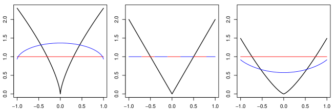
Figure 1: Variances $\sigma^{2}(t)$ of the Gaussian representations of the variogram $\gamma({h})=\lvert h/s\rvert^{\alpha}$ on the domain $K=[-1,1]$. The plots show the variance for the original representation with $W_{0}(0)=0$ (black), the minimal $K$-stationary representation (red) and the $\lambda$-modified representation with $\lambda=\text{Unif}(\text{Ex}(K))$ (blue). For $\alpha=1$ the last two coincide. The scale $s>0$ is chosen such that the variance of the minimal $K$-stationary representation (red) is normalized to 1.

$\bm{\lambda}$-modified $K$-stationary original $\bm{\alpha=0.7}$ $\bm{\alpha=1.0}$ $\bm{\alpha=1.3}$

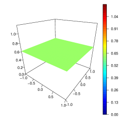
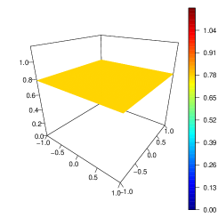
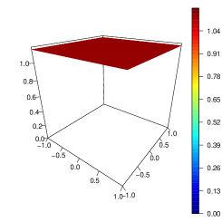
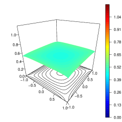
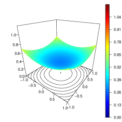
Figure 2: Variances $\sigma^{2}(t)$ of the Gaussian representations of the variogram $\gamma(\bm{h})=\lVert\bm{h}/\sqrt{2}\rVert^{\alpha}$ on the domain $K=[-1,1]^{2}$ for $\alpha\in\{0.7,1.0,1.3\}$ (left to right). The plots show the variance for the original representation with $W_{0}(\bm{0})=0$, the minimal $K$-stationary representation and the $\lambda$-modified representation with $\lambda=\text{Unif}(\text{Ex}(K))$ (top to bottom). Minimality of the $K$-stationary representation refers to the minimal ball $B_{\sqrt{2}}(\bm{0})$ containing $K$.

Example 3.9.

Let $\gamma({h})=\lvert{h}/s\rvert^{\alpha}$, $\alpha\in(0,2)$, $s>0$, be the family of fractional Brownian motion variograms in dimension $1$. Collectively, the results from Examples 3.2 and 3.6, Proposition 3.8 (b) provide a full description of the intrinsically stationary Gaussian representations $W_{\min}$ of $\gamma$ on the domain $[-R,R]\subset\mathbb{R}$ that minimize the maximal variance therein.

• For $\alpha\in[1,2)$ it is given by the minimizing measure $\lambda_{\min}=\frac{1}{2}(\delta_{-R}+\delta_{R})$ as described in Proposition 3.1 and Example 3.2. If $W_{0}$ is any intrinsically stationary Gaussian representation of $\gamma$, it can be obtained as the $\lambda_{\min}$-modified process

  $$W_{\min}(x)=W_{0}(x)-\frac{1}{2}(W_{0}(-R)+W_{0}(R)),\quad x\in[-R,R].$$ (14)

• For $\alpha\in(0,1]$ Proposition 3.8 (b) tells us that the covariance function of $W_{\min}$ is

  $$C_{\min}(x,y)=\frac{A_{\alpha,1}-\lvert x-y\lvert^{\alpha}}{2s^{\alpha}},\quad x,y\in[-R,R],$$ (15)

  which is the minimal $K$-stationary representation of $\gamma$ on $K=B_{R}(0)=[-R,R]$.

This description was already obtained by Matheron (1974). In particular, the case $\alpha=1$ in dimension $1$ is very special in the sense that (i) $d$-dimensional balls and $d$-dimensional hyperrectangles are the same and (ii) the functions $h\mapsto\lvert h/s\rvert^{\alpha}$, $s>0$, are both concave and convex on $[0,\infty)$ for $\alpha=1$. This leads to the situation that the minimizing representation can be obtained either way. The covariance of (14) is precisely (15) for $\alpha=1$.

As an illustration of the different cases, Figure 2 shows the variances of the original representation (with $W_{0}(0)=0$), the $\lambda$-modified representation (with $\lambda=\frac{1}{2}(\delta_{-1}+\delta_{1})$) and the minimal $K$-stationary representation of Gaussian random fields on $K=[-1,1]$ with variogram $\gamma(h)=\lvert h/s\rvert^{\alpha}$ for $\alpha\in\{0.7,1,1.3\}$.

Example 3.10.

Let $\gamma(\bm{h})=\lVert\bm{h}/s\rVert^{\alpha}$, $\alpha\in(0,2)$, $s>0$, be the family of variograms of fractional Brownian sheets in dimension $d\geq 2$ and consider the (hyper-)rectangular simulation domain $K=\prod_{i=1}^{d}[-R_{i},R_{i}]$. Again we are interested in the intrinsically stationary Gaussian representation $W_{\min}$ of $\gamma$ on the domain $K\subset\mathbb{R}^{d}$ that minimize the maximal variance therein.

• When $\alpha\in[1,2)$, still Proposition 3.1 and Example 3.2 provide the minimizing measure

  $$\lambda_{\min}=\frac{1}{2^{d}}\sum_{A\subset\{1,\dots,d\}}\delta_{\bm{v}_{A}},\quad\bm{v}_{A}=(\sigma^{A}_{i}R_{i})_{i=1}^{d},\quad\sigma^{A}_{i}=\begin{cases}+1&i\in A\\ -1&i\not\in A\end{cases},$$

  and $W_{\min}$ can be obtained as the $\lambda$-modified process from (11).

• However, for $\alpha\in(0,1)$, we do not know the minimizing measure $\lambda_{\min}$ or the corresponding covariance $C_{\min}$, not even if we replace the domain $K$ by the $d$-dimensional ball $B_{R}(\bm{0})$. At least, Proposition 3.8 identifies on $\widetilde{K}=B_{R}(\bm{0})$ the minimal $\widetilde{K}$-stationary Gaussian representations of the variogram $\gamma$ for $\alpha\in(0,2)$. For $R=(R_{1}^{2}+\dots+R_{d}^{2})^{1/2}$ the domain $\widetilde{K}=B_{R}(\bm{0})$ is the smallest ball that contains $K$. Therefore, the covariance

  $$C(\bm{x},\bm{y})=\frac{A_{\alpha,d}R^{\alpha}-\big{\lVert}(\bm{x}-\bm{y})\big{\rVert}^{\alpha}}{2s^{\alpha}},\quad\bm{x},\bm{y}\in K,$$ (16)

  also describes a $K$-stationary Gaussian representation of $\gamma$, but we do not know if it is minimal among $K$-stationary Gaussian representations of $\gamma$ on $K$. However, Figure 2 illustrates that it is certainly not minimal among general Gaussian representations of $\gamma$. In each situation, the $\lambda$-modified processes (11) has an even smaller maximal variance on $K$ than the $K$-stationary process derived from (16). While this is not a surprise for $\alpha=1$ or $\alpha=1.3$, where we know that (11) is minimal, it seems quite remarkable how much the maximal variance of (11) is reduced even in the case $\alpha=0.7$ compared to the $K$-stationary process from (16). This is a major difference to the 1-dimensional case that we considered in Example 3.9, where the $K$-stationary process provides the minimal representation.

Remark 3.11.

In the literature, there are different other terms related to the concept of $K$-stationarity. In Gneiting et al. (2001), for instance, a locally equivalent stationary covariance is defined as covariance function $C$ on $\mathbb{R}^{d}\times\mathbb{R}^{d}$ such that $C(\bm{x},\bm{y})$ only depends on $\bm{x}-\bm{y}$ for all $\bm{x},\bm{y}\in\mathbb{R}^{d}$ and

$$C(\bm{x},\bm{y})=C(\bm{0})-\frac{1}{2}\gamma(\bm{x}-\bm{y}),\quad\bm{x},\bm{y}\in K.$$ (17)

In general, this assumption is stronger than the one in our definition, as it additionally requires that the locally defined covariance function $C$ on $K\times K$ can be extended to a stationary covariance function on $\mathbb{R}^{d}\times\mathbb{R}^{d}$. There are numerous examples of variograms $\gamma$ and corresponding functions of the form (17) that are positive definite on a small (potentially discrete and finite) domain $K$ for sufficiently large $C(\bm{0})$, but cannot be extended to a positive definite function on $\mathbb{R}^{d}\times\mathbb{R}^{d}$. In case of an isotropic variogram and a domain of the type $K=B_{R}(\bm{0})$ for some $R>0$, i.e. in the case considered in Proposition 3.8, however, such an extension is always possible by Rudin’s Theorem (Rudin, 1970). Thus, the terms locally equivalent stationary covariance and covariance of a $K$-stationary representation are equivalent in case $K=B_{R}(\bm{0})$.

3.4 Discretization effects

In our examples above, we always considered processes on convex $d$-dimensional domains $K$ with non-trivial interior (such as $d$-dimensional hyperrectangles or $d$-dimensional balls of some radius). Indeed the regions of interest are usually of such kind. On the other hand, the simulation domain $K$ in a computer experiment is necessarily a finite set of points $K=\{\bm{x}_{i}\}_{i=1,\dots,N}$ (such as a subgrid of a hyperrectangle) and the minimizing measure $\lambda_{\min}$ can depend on this choice of discretization. In case that the variogram $\gamma$ is convex, not much changes. Proposition 3.1 still applies and in particular, if the discritization consists of a subgrid of some rectangular domain, the minimizing measure $\lambda_{\min}$ will be equal to the uniform distribution on the vertices of the chosen subgrid. The modified process $W$ as in (11) still yields the minimal representation of the variogram $\gamma$.

It is again the case of a non-convex variogram $\gamma$, which is more intricate. First, we know that Proposition 3.5 also still applies and typically, we can reduce the maximal variance by a significant amount by the same strategy as before, i.e. by considering the modification $W$ in (11) instead of the original representation $W_{0}$. In the example of an $\alpha$-fractional Brownian sheet we found this strategy useful when $\alpha$ is close to 1. Secondly, since we discretized our space, it is usually possible to solve

$$\int_{K}\gamma(\bm{x}-\bm{y})\lambda_{0}(\mathrm{d}\bm{y})=1,\qquad\bm{x}\in K$$

explicitly for $\lambda_{0}$. If $\lambda_{0}$ is a non-negative measure (and not a signed measure), normalizing $\lambda_{0}$ so that it becomes a probability measure will then provide the minimal ($K$-stationary) solution $\lambda_{\min}$, see Matheron (1974), page 8. In case of an $\alpha$-fractional Brownian sheet, we found this strategy useful for $d=1$ or $\alpha$ close to zero and our numerical experiments led us to the following conjecture.

Conjecture 3.12.

Let $K=\{\bm{x}_{i}\}_{i=1,\dots,N}$ be a finite set of distinct points in $\mathbb{R}^{d}$, which contains at least two elements. Set $\bm{\Gamma}_{ij}=\lVert\bm{x}_{i}-\bm{x}_{j}\rVert^{\alpha}$, $i,j=1,\dots,N$, $\alpha\in(0,1]$ and let $\bm{e}\in\mathbb{R}^{N}$ be the vector, whose entries are all equal to $1$.

1. For $d=1$ and $\alpha\in(0,1]$ all entries of $\bm{\Gamma}^{-1}\bm{e}$ are non-negative (we write $\bm{\Gamma}^{-1}\bm{e}\geq 0$).

2. For $d\geq 2$ there exists $\alpha_{\text{critical}}=\alpha_{\text{critical}}(K)\in(0,1]$, such that $\bm{\Gamma}^{-1}\bm{e}\geq 0$ for $\alpha\in(0,\alpha_{\text{critical}}]$.

3. We have $\alpha_{\text{critical}}(K)=1$ if and only if the points in $K$ are collinear.

For the remaining cases the minimal solution $\lambda_{\min}=\sum_{i=1}^{N}\lambda_{i}\delta_{\bm{x}_{i}}$ can be obtained from the solution $\bm{\lambda}\in\mathbb{R}^{N}$ of the optimization problem

$$\min_{\bm{\lambda}}\quad\max_{i=1}^{N}\frac{1}{2}(\bm{\lambda}-\bm{e}^{i})^{\text{T}}(-\bm{\Gamma})(\bm{\lambda}-\bm{e}^{i})\qquad\text{subject to}\qquad\bm{e}^{\text{T}}\bm{\lambda}=1,\quad\bm{\lambda}\geq\bm{0},$$ (18)

where the vector $\bm{e}^{i}$ is the $i$-th unit vector in $\mathbb{R}^{N}$, the matrix $\bm{\Gamma}$ has entries $\bm{\Gamma}_{ij}=\gamma(\bm{x}_{i}-\bm{x}_{j})$ and $\bm{e}=\sum_{i=1}^{N}\bm{e}^{i}$. This is a non-linear convex optimization problem that can be solved via standard optimization techniques.

4 Numerical results

Table 1: Simulation scenarios in dimension 1 on the interval $K=[-1,1]$ for Brown-Resnick processes associated to the variogram $\gamma({h})=\lvert h/s\rvert^{\alpha}$, see Section 4. The scale $s$ is obtained from (19).

	Feature of	Minimal Gaussian	Scale 1	Scale 2	Scale 3
	variogram	representation	$\sigma^{2}_{K}=0.5$	$\sigma^{2}_{K}=1$	$\sigma^{2}_{K}=2$
$\alpha=0.7$	concave	$K$-stationary	$s=0.818$	$s=0.304$	$s=0.113$
$\alpha=1.0$	linear	$K$-stat. / $\lambda=\text{Unif}(\text{Ex}(K))$	$s=1.000$	$s=0.500$	$s=0.250$
$\alpha=1.3$	convex	$\lambda=\text{Unif}(\text{Ex}(K))$	$s=1.253$	$s=0.735$	$s=0.431$

Our numerical study focuses on Brown-Resnick processes on the hyperrectangle $K=[-1,1]^{d}$ in dimensions $d\in\{1,2\}$ with the underlying variograms belonging to the fractional Brownian sheet family $\gamma(\bm{h})=\lVert\bm{h}/s\rVert^{\alpha}$. It compares the performance of the threshold stopping algorithms that are based on

1. the original Gaussian representation $W_{0}$ of the variogram $\gamma$ with $W_{0}(\bm{0})=0$,

2. the minimal $K$-stationary Gaussian representation from (16),

3. the $\lambda$-modified Gaussian representation from (11).

In dimension 1 we fix the actual simulation domain as the grid $\{-1,-0.996,\dots,1\}\subset[-1,1]=K$ that consists of 501 equally spaced points and vary both the smoothness parameter $\alpha\in(0,2)$ and scale $s>0$ as shown in Table 1. In each column the scale is chosen such that the minimal $K$-stationary Gaussian representation of the variogram (15) has the same variance $\sigma^{2}_{K}$ across the domain $K=[-1,1]$, that is

$$s=\bigg{(}\frac{1}{{2}\sqrt{\pi}\sigma^{2}_{K}}{\Gamma\Big{(}\frac{2-\alpha}{2}\Big{)}\Gamma\Big{(}\frac{1+\alpha}{2}\Big{)}}\bigg{)}^{1/\alpha},\quad\sigma^{2}_{K}\in\{0.5,1,2\}.$$ (19)

In the case $\alpha=1$ one could equivalently fix the scale as $s=1$ and vary the domain $K=[-R,R]$ across $R=1$, $R=2$ and $R=4$. In dimension 2 we fix the simulation domain as the grid $\{-1,-0.9,\dots,1\}^{2}\subset[-1,1]^{2}=K$ that consists of $21\times 21$ points and consider as a variogram the classical two-dimensional Brownian sheet variogram $\gamma(\bm{h})=(2\sqrt{2}/\pi)\lVert\bm{h}\rVert$ where $\alpha=1$. The scale $s=\pi/{(2\sqrt{2})}$ is chosen in such a way that the variance $\sigma^{2}_{K}$ of the associated $K$-stationary representation from (16) equals 1.

All simulation experiments are repeated $50\,000$ times. Based on the $50\,000$ simulated realizations of $Z^{(T)}$ and $50\,000$ independent realizations of the corresponding spectral process $V$, we estimate the benchmark simulation error $\mathcal{P}_{K,\tau}$ according to (5). The estimated errors are reported in Table 3 for dimension 1 and Table 3 for dimension 2. The smallest error term in each scenario is always marked bold. To ensure consistency across the different scenarios, we first fix $\tau_{\text{$\lambda$-mod}}$ such that the resulting benchmark error term $\widehat{\mathcal{P}}_{K,\tau}$ assumes a value around 0.1, i.e. the third column in Tables 3 and 3 is always fixed (up to small deviations). To ensure a fair comparison of the different algorithms, we then choose the other thresholds $\tau_{\text{orig}}$, $\tau_{\text{$K$-stat}}$ in such a way that the mean number $\mathbb{E}T_{K,\tau}$ of Gaussian processes that need to be simulated to obtain one single approximation to the Brown-Resnick process stays fixed within each scenario (up to relative deviations smaller than $1\%$).

Table 2: Benchmark error terms ${\widehat{\mathcal{P}}}_{K,\tau}$ for threshold stopping algorithms based on Gaussian representations for the simulation scenarios of Table 1, where $\alpha\in\{0.7,1.0,1.3\}$, see Section 4.

		Original	$\bm{K}$-	$\bm{\lambda=}\text{Unif}(\text{Ex}(K))$
Scenario		definition	stationary	modification
Scale 1	$\alpha=0.7$	0.19	0.05	0.10
	$\alpha=1.0$	0.17	0.10	0.10
	$\alpha=1.3$	0.16	0.17	0.10
Scale 2	$\alpha=0.7$	0.25	0.04	0.11
	$\alpha=1.0$	0.22	0.11	0.11
	$\alpha=1.3$	0.20	0.20	0.10
Scale 3	$\alpha=0.7$	0.32	0.03	0.10
	$\alpha=1.0$	0.24	0.11	0.09
	$\alpha=1.3$	0.21	0.24	0.10

Table 3: Benchmark error terms ${\widehat{\mathcal{P}}}_{K,\tau}$ for threshold stopping algorithms based on Gaussian representations for the simulation of Brown-Resnick processes on the square $K=[-1,1]^{2}$ associated to the variogram $\gamma(\bm{h})=(2\sqrt{2}/\pi)\lVert\bm{h}\rVert$.

		Original	$\bm{K}$-	$\bm{\lambda=}\text{Unif}(\text{Ex}(K))$
Scenario		definition	stationary	modification
$\sigma^{2}_{K}=1$, $\alpha=1.0$		0.23	0.30	0.10

The results in Tables 3 and 3 allow us to compare the performance of the different algorithms according to the error term ${\widehat{\mathcal{P}}}_{K,\tau}$ within a given scenario $(\alpha,s)$. As explained in Example 3.9, in dimension 1 we know for each scenario $(\alpha,s)$ which of the Gaussian representations of the variogram $\gamma(h)=\lvert h/s\rvert^{\alpha}$ leads to the minimal maximal variance across the simulation domain $[-1,1]$. It only depends on the value of $\alpha$ as listed in Table 1. Indeed the simulation results in Table 3 show that the smallest error term ${\widehat{\mathcal{P}}}_{K,\tau}$ is always attained by the algorithm that corresponds to the minimal representation. This confirms our previous theoretical considerations on the influence of the maximal variance of the spectral process on the performance of the threshold stopping algorithms. In dimension 2 we focus on the classical scenario of a two-dimensional Brownian sheet. As we can see from Table 3 and as anticipated, simulations via the threshold stopping algorithm based on the $\lambda$-modified representation exhibit smaller errors than simulations based on the $K$-stationary representation and simulations based on the original definition. This observation is well in line with our theoretical considerations, since the maximal variance of the $\lambda$-modified representation is the smallest among those three (cf. Figure 2). It is even minimal in the sense of Problem 1, cf. Proposition 3.1. In case $\alpha=1.3$ in dimension 1 and $\alpha=1$ in dimension $2$, the threshold-stopping algorithm that is based on the $K$-stationary representation performs slightly worse than the original definition. Here, Figures 2 and 2 show (for both cases) that the variance of the original field is much smaller than the $K$-stationary variance on a large proportion of the relevant domain $[-1,1]^{d}$, which can explain this phenomenon as a reasonable subasymptotic effect. Otherwise, the ranking of the threshold stopping algorithms according to the error terms even corresponds precisely to the ranking of the maximal variance on $[-1,1]$ for each of the remaining scenarios in dimension 1.

In addition, we compare the performance of the above threshold stopping algorithms that are based on Gaussian processes to the performance of three other established algorithms for simulation of max-stable processes, namely

1. the random shift approach (cf. Oesting et al. (2012)), a threshold stopping algorithm, where the original log-Gaussian spectral process $V^{\text{(orig)}}$ is additionally shifted uniformly across the (finite!) simulation domain $K=\{\bm{x}_{1},\ldots,\bm{x}_{N}\}$, i.e. its spectral process is

   $$V^{\text{(shift)}}(\bm{x})=V^{\text{(orig)}}(\bm{x}-\bm{S}),\quad\bm{x}\in K=\{\bm{x}_{1},\ldots,\bm{x}_{N}\},$$

   where ${\bm{S}}$ is uniformly distributed on $K=\{\bm{x}_{1},\ldots,\bm{x}_{N}\}$ and independent of $V^{\text{(orig)}}$.

2. the Dieker-Mikosch approach (cf. Dieker and Mikosch (2015) and Dombry et al. (2016)), another threshold stopping algorithm, which is based on the (sum-)normalized spectral process of the form

   $$V(\bm{x})=N\frac{\exp(W^{\text{(orig)}}(\bm{x}-\bm{S}))}{\sum_{k=1}^{N}\exp(W^{\text{(orig)}}(\bm{x}-\bm{x}_{k}))},\quad\bm{x}\in K=\{\bm{x}_{1},\ldots,\bm{x}_{N}\},$$ (20)

   where ${\bm{S}}$ is again uniformly distributed on $K=\{\bm{x}_{1},\ldots,\bm{x}_{N}\}$ and independent of $W^{\text{(orig)}}$.

3. the extremal functions approach (cf. Dombry et al. (2016)) with exact simulation taking place on a subset of $N_{\text{extrfun}}$ pre-specified equi-spaced locations in the simulation domain only.

To ensure a fair comparison, the thresholds for the random shift approach and the Dieker-Mikosch algorithm are again chosen in such a way that the mean number $\mathbb{E}T_{K,\tau}$ of Gaussian processes is fixed within each scenario (up to relative deviations smaller than $1\%$). Likewise, we fix the expected number of simulated Gaussian processes for the extremal functions approach, for which it corresponds to the expected number $N_{\text{extrfun}}$ of locations for which exact simulation is ensured (cf. Dombry et al., 2016). Since all scales in Table 3 seem to reproduce a similar qualitative behaviour, we focus in this experiment on the scenarios in Table 1 corresponding to Scale 1 ($\sigma_{K}^{2}=0.5$) and explore a slightly larger range of $\alpha\in\{0.1,0.4,\dots,1.9\}$. The results are reported in Table 4 and plotted in Figure 3.

Table 4: Benchmark error terms ${\widehat{\mathcal{P}}}_{K,\tau}$ for threshold stopping algorithms based on Gaussian representations and three further algorithms for the simulation scenarios of Table 1 with Scale 1 ($\sigma_{K}^{2}=0.5$), see Figure 3 for an illustration.

		Original	$\bm{K}$-	$\bm{\lambda=}\text{Unif}(\text{Ex}(K))$	Random	Dieker-	Extremal
Scenario		definition	stationary	modification	shift	Mikosch	functions
Scale 1	$\alpha=0.1$	0.244	0.007	0.098	0.263	0.005	0.899
	$\alpha=0.4$	0.204	0.018	0.095	0.245	0.003	0.822
	$\alpha=0.7$	0.186	0.051	0.103	0.265	0.006	0.686
	$\alpha=1.0$	0.168	0.102	0.101	0.236	0.017	0.521
	$\alpha=1.3$	0.161	0.172	0.102	0.223	0.037	0.364
	$\alpha=1.6$	0.130	0.241	0.102	0.171	0.063	0.231
	$\alpha=1.9$	0.109	0.362	0.101	0.121	0.094	0.210

Average Error Probability ${\widehat{\mathcal{P}}}_{K,\tau}$
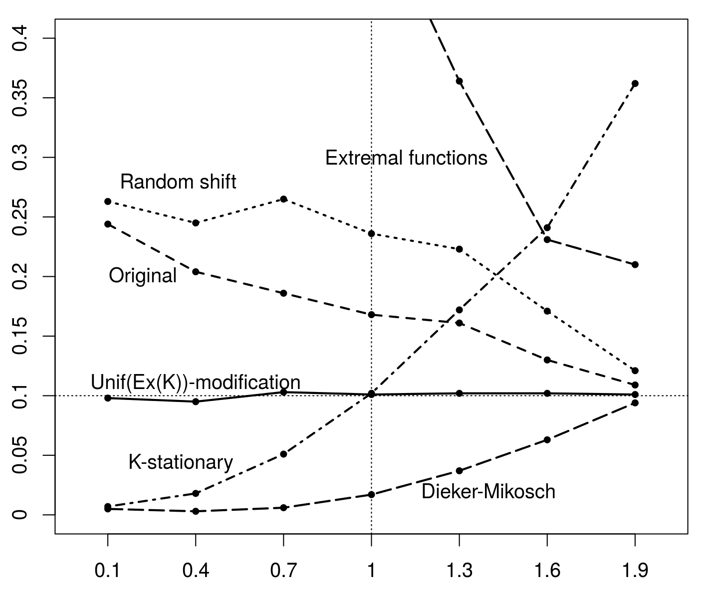
	$\alpha$

Figure 3: Benchmark error terms ${\widehat{\mathcal{P}}}_{K,\tau}$ for threshold stopping algorithms based on Gaussian representations (“Original”, “Unif(Ex(K))-modification”, “K-stationary”) and three further algorithms (“Random shift”, “Dieker-Mikosch”, “Extremal functions”) for the simulation scenarios of Table 1 with Scale 1 ($\sigma_{K}^{2}=0.5$), see Table 4 for the estimated values.

A first observation (that we found surprising at first sight) is the poor performance of the extremal functions approach and the strong performance of the Dieker-Mikosch approach in this experiment. We did not expect this previously, since for exact simulation the extremal functions approach always outperforms the Dieker-Mikosch algorithm in terms of expected number of simulated Gaussian processes, see Dombry et al. (2016) and Oesting and Strokorb (2018), i.e. one should prefer the extremal functions approach in this case. We conclude that allowing for a simulation error makes the Dieker-Mikosch approach competitive again with other methods. Intuitively, this can be explained by its spectral functions (20) being bounded and probabilistically homogeneous in space which makes its convergence rate be quite fast at the beginning. While the random shift approach also enforces homogeneity of the spectral functions, this is however done in this case at the cost of increasing the maximal variance of the spectral functions, which explains why its performance is even worse than the performance of the original Gaussian representation. Generally, the three threshold-stopping algorithms that are based on Gaussian representation lie all inbetween the random shift approach (apart from too high values of $\alpha$, when the $K$-stationary approach is the worst) and the Dieker-Mikosch approach. Among them, one can also see the phase transition at $\alpha=1$ between the $K$-stationary approach performing better for $\alpha<1$ and the $\lambda$-modification taking over for $\alpha>1$ quite well. As $\alpha$ gets close to zero, the $K$-stationary approach and the Dieker-Mikosch approach show a similar error rate, whereas the $\lambda$-modification and the Dieker-Mikosch approach perform similarly as $\alpha$ gets close to $2$.

5 Discussion

Efficient simulation of Brown-Resnick processes is an important task that is often needed to describe the extremal behaviour of spatial random fields. As exact simulation of such processes can be very time-consuming, in particular when the simulation domain consists of a large number of points, it is often necessary to resort to the simulation of approximations of these processes. This can be done by either cutting an exact algorithm short or by running an inexact stopping algorithm. A priori it is unclear which algorithm will lead to the smallest error term for a fixed simulation time or vice versa. Our focus here lies on the classical threshold-stopping algorithm (Schlather, 2002), where we consider different (log-)Gaussian spectral representations. Trying to mitigate the problem of the occurrence of exessively large variances of the spectral functions has lead us to the following optimization problem:

Minimization problem. Among Gaussian processes with prescribed variogram $\gamma$,
find a process $W$ such that $\sup_{x\in K}\mathrm{Var}(W(x))$ is minimal.

This is a difficult mathematical problem that has been of independent interest for the case of $K$-stationary solutions in geostatistics (or locally equivalent stationary solutions, respectively), see e.g. Gneiting et al. (2001); Gneiting (1999, 2000); Stein (2001); Chilès and Delfiner (2012); Matheron (1973). To the best of our knowledge, an explicit solution is known only in very few cases such as for the variogram of a fractional Brownian motion on an interval (cf. Example 3.9 stating Matheron (1974)). Solutions also depend quite heavily on the geometry of the simulation domain $K$. Generally, Matheron’s (1974) contribution does not seem to have received very much attention in the literature so far.

Here, we first make his description of a solution for convex variograms more explicit for symmetric domains (cf. Proposition 3.1) and second, we prove that the strategy that is employed for symmetric domains can even be applied to most practically relevant non-convex variograms on hyperrectangular domains in order to achieve a substantial reduction of the maximal variance $\sup_{x\in K}\mathrm{Var}(W(x))$, albeit not a minimal solution (cf. Proposition 3.5). We also consider discretization effects and conjecture for the fractional Brownian sheet family with variogram $\lVert h\rVert^{\alpha}$ the existence of a critical value of $\alpha$, below of which the solution to the minimization problem is $K$-stationary (cf. Conjecture 3.12).

One of the nice features of the variance reduction is that it can be very easily implemented. Our simulation study confirms that the proposed modification of threshold-stopping algorithms that are based on a Gaussian representation can lead to significant improvements of the probability that no approximation error occurs while the expected running time is fixed. We expect similar performance improvements also for other features, e.g. when other types of errors are considered, cf. Oesting and Strokorb (2018). Further improvements are possible, when taking into account discretization effects, i.e. modifying the Gaussian representation of the variogram $\gamma$ according to (6) using the discrete minimizing measure (18). In our numerical study, we always considered a relatively dense grid, such that discretization effects (not reported) did not play a significant role. However, we conclude from further experiments (not reported) that they can become relevant for coarser designs.

A comparison with three other established simulation algorithms demonstrates that our approach can compete with the (potentially exact) extremal functions method (Dombry et al., 2016) and always outperforms the random shift modification (Oesting et al., 2012) due to its increased variance. We were unable to detect a scenario, in which our approach would outperform the Dieker-Mikosch algorithm (Dieker and Mikosch, 2015). The latter seems to converge relatively fast at the beginning stages of a simulation due to the boundedness and probabilistic homogeneity of the spectral functions in this threshold-stopping approach. However, when increasing the required accuracy, one should expect a phase transition, in which the Dieker-Mikosch approach performs better first, before the extremal functions approach takes over again. If we consider only the threshold-stopping approach based on Gaussian spectral representations, the proposed variance reduction leads to the best performances as expected. Further comparisons of different simulation algorithms are beyond the scope of this paper, but will be addressed in Oesting and Strokorb (2018).

Appendix A Proofs

A.1 Proofs for Section 2

Proposition A.1.

Let $\{W_{1}(\bm{x}),\bm{x}\in K\}$ and $\{W_{2}(\bm{x}),\bm{x}\in K\}$ be two centered Gaussian processes with a.s. bounded sample paths and bounded variance functions $\sigma_{i}^{2}(\bm{x})=\mathrm{Var}(W_{i}(\bm{x}))$, $i=1,2$. Further, let $\sigma_{1,\max}^{2}<\sigma_{2,\max}^{2}$ where $\sigma_{i,\max}^{2}=\sup_{\bm{x}\in K}\sigma_{i}^{2}(\bm{x})<\infty$ for $i=1,2$. Then, for any function $y\in C(K)$

$$\lim_{u\to\infty}\frac{\mathbb{P}\big{(}\sup_{\bm{x}\in K}W_{1}(\bm{x})-\sigma_{1}^{2}(\bm{x})/2-y(\bm{x})>u\big{)}}{\mathbb{P}\big{(}\sup_{\bm{x}\in K}W_{2}(\bm{x})-\sigma_{2}^{2}(\bm{x})/2-y(\bm{x})>u\big{)}}=0.$$

Proof of Proposition A.1.

By Proposition 1 in Debicki et al. (2010), for $i=1,2$, we have

$$-\log\mathbb{P}\bigg{(}\sup_{\bm{x}\in K}W_{i}(\bm{x})-\sigma_{i}^{2}(\bm{x})/2-y(\bm{x})>u\bigg{)}\sim-\log\mathbb{P}\bigg{(}\sup_{\bm{x}\in K}W_{i}(\bm{x})>u\bigg{)}\sim\frac{u^{2}}{2\sigma^{2}_{i,\max}}$$

as $u\to\infty$. Consequently, for each $\varepsilon>0$, there is some $u_{i}(\varepsilon)>0$ such that for all $u>u_{i}(\varepsilon)$

$$\exp\bigg{(}-\frac{u^{2}(1+\varepsilon)}{2\sigma_{i,\max}^{2}}\bigg{)}\leq{}\mathbb{P}\bigg{(}\sup_{\bm{x}\in K}W_{i}(\bm{x})-\sigma_{i}^{2}(\bm{x})/2-y(\bm{x})>u\bigg{)}\leq{}\exp\bigg{(}-\frac{u^{2}(1-\varepsilon)}{2\sigma_{i,\max}^{2}}\bigg{)}.$$

Now, let $\varepsilon>0$ be sufficiently small such that $(1-\varepsilon)\sigma^{2}_{2,\max}>(1+\varepsilon)\sigma^{2}_{1,\max}$. Then, for all $u>\max\{u_{1}(\varepsilon),u_{2}(\varepsilon)\}$, we have

$$\frac{\mathbb{P}\big{(}\sup_{\bm{x}\in K}W_{1}(\bm{x})-\sigma_{1}^{2}(\bm{x})/2-y(\bm{x})>u\big{)}}{\mathbb{P}\big{(}\sup_{\bm{x}\in K}W_{2}(\bm{x})-\sigma_{2}^{2}(\bm{x})/2-y(\bm{x})>u\big{)}}\leq{} \exp\bigg{(}-\frac{u^{2}}{2}\cdot\bigg{(}\frac{1-\varepsilon}{\sigma^{2}_{1,\max}}-\frac{1+\varepsilon}{\sigma^{2}_{2,\max}}\bigg{)}\bigg{)},$$

which implies the assertion. ∎

A.2 Proofs for Section 3

Proof of Proposition 3.1.

First note that $\text{Ex}(K)$ is a (locally compact) homogeneous space with respect to the action of $\text{Sym}(\text{Ex}(K))\subset O(\mathbb{R}^{d})$ and so a unique normalized left invariant Haar measure $\lambda$ exists on $\text{Ex}(K)$ which we call uniform distribution, cf. e.g. Nachbin (1976) or Mardia and Khatri (1977). Its support $\text{Supp}(\lambda)=\text{Ex}(K)$ is necessarily a subset of $\text{Ex}(K)$, which establishes (8) for $\lambda$. Further, observe that the assignment

$$\bm{x}\mapsto\int_{K}\gamma(\bm{x}-\tilde{\bm{y}})\,\lambda(\mathrm{d}\tilde{\bm{y}})=\int_{\text{Ex}(K)}\gamma(\bm{x}-\tilde{\bm{y}})\,\lambda(\mathrm{d}\tilde{\bm{y}})$$

is also a convex function (since $\gamma$ is convex). In particular, it attains its maximal value $m$ on $K$ for some $v\in\text{Ex}(K)$. Since $\text{Sym}(\text{Ex}(K))\subset O(\mathbb{R}^{d})$ acts transitively on $\text{Ex}(K)$, any element in $\text{Ex}(K)$ can be represented as $\bm{M}\bm{v}$ for some $\bm{M}\in O(\mathbb{R}^{d})$. Since $\gamma(\bm{h})$ depends only on $\lVert\bm{h}\rVert$, this gives

$$\int_{\text{Ex}(K)}\gamma(\bm{M}\bm{v}-\tilde{\bm{y}})\,\lambda(\mathrm{d}\tilde{\bm{y}})=\int_{\text{Ex}(K)}\gamma(\bm{M}\bm{v}-\bm{M}\tilde{\bm{y}})\,\lambda(\mathrm{d}\tilde{\bm{y}})=\int_{\text{Ex}(K)}\gamma(\bm{v}-\tilde{\bm{y}})\,\lambda(\mathrm{d}\tilde{\bm{y}}).$$

So, in fact, all elements of $\text{Ex}(K)$ attain this maximal value $m$, which implies

$$\int_{K}\int_{K}\gamma(\tilde{\bm{x}}-\tilde{\bm{y}})\,\lambda(\mathrm{d}\tilde{\bm{x}})\,\lambda(\mathrm{d}\tilde{\bm{y}})=\int_{\text{Ex}(K)}\int_{\text{Ex}(K)}\gamma(\tilde{\bm{x}}-\tilde{\bm{y}})\,\lambda(\mathrm{d}\tilde{\bm{x}})\,\lambda(\mathrm{d}\tilde{\bm{y}})=\int_{\text{Ex}(K)}m\lambda(\mathrm{d}\tilde{\bm{y}})=m.$$

Finally, this gives

$$\int_{K}\gamma(\bm{x}-\tilde{\bm{y}})\,\lambda(\mathrm{d}\tilde{\bm{y}}) \leq m\leq\int_{K}\int_{K}\gamma(\tilde{\bm{x}}-\tilde{\bm{y}})\,\lambda(\mathrm{d}\tilde{\bm{x}})\,\lambda(\mathrm{d}\tilde{\bm{y}})$$

for all $\bm{x}\in\text{Ex}(K)$, as desired (cf. Condition (9)). ∎

Proof of Lemma 3.4.

First note that (i) is equivalent to $\psi$ being negative definite in the sense of (12). The equivalence “(i) $\Leftrightarrow$ (ii)” is then immediate from Corollary 5.1.8 of Berg et al. (1984) (page 150 therein) and the fact that $(\mathbb{R},\mathbb{R}_{+},x^{2})$ is a Schoenberg triple, cf. Example 5.1.3 of Berg et al. (1984) (page 146 therein). Second, the equivalence “(i) $\Leftrightarrow$ (iii)” follows from Corollary 4.6.8 of Berg et al. (1984) (page 133 therein) and the 2-divisibility of the semigroup $(\mathbb{R}_{+},+)$. ∎

Lemma A.2.

Let $\psi:\mathbb{R}_{+}\rightarrow\mathbb{R}$ be $n$-alternating up to $n\leq 2$ and $0\leq x\leq R$ as well as $0\leq x_{i}\leq R_{i}$ for $i=1,\dots,d$. Then the following inequalities hold true for any $a\geq 0$.

1. $\psi(a+(R-x)^{2})+\psi(a+(R+x)^{2})\leq\psi(a+R^{2})+\psi(a+3R^{2})$

2. $\sum_{A\subset\{1,\dots,d\}}\psi(a+\sum_{i\in A}(x_{i}-R_{i})^{2}+\sum_{j\in A^{c}}(x_{j}+R_{j})^{2})$
   $\phantom{(a)}\leq\sum_{A\subset\{1,\dots,d\}}\psi(a+3\sum_{i\in A}R_{i}^{2}+\sum_{j\in A^{c}}R_{j}^{2})$

Proof.

1. By the alternation properties of $\psi$, we have that

   $$\psi(a+(R-x)^{2})+\psi(a+(R+x)^{2})-\psi(a+R^{2})-\psi(a+3R^{2})$$

   $$\leq{} \psi(a+(R-x)^{2})+\psi(a+(R+x)^{2})-\psi(a+R^{2})-\psi(a+R^{2}+2x^{2})$$

   $$={} \Delta_{2Rx-x^{2}}\Delta_{2Rx+x^{2}}\psi(a+(R-x)^{2})\leq 0$$

2. The assertion follows by induction on $d$. For $d=1$ it is evident from (a). For the step from $d$ to $d+1$ note that

   $$\sum_{A\subset\{1,\dots,d+1\}}\psi\bigg{(}a+\sum_{i\in A}(x_{i}-R_{i})^{2}+\sum_{j\in A^{c}}(x_{j}+R_{j})^{2}\bigg{)}$$

   $$={} \sum_{B\subset\{1,\dots,d\}}\psi\bigg{(}a+\sum_{i\in B}(x_{i}-R_{i})^{2}+\sum_{j\in B^{c}}(x_{j}+R_{j})^{2}+(x_{d+1}-R_{d+1})^{2}\bigg{)}$$

   $$+\sum_{B\subset\{1,\dots,d\}}\psi\bigg{(}a+\sum_{i\in B}(x_{i}-R_{i})^{2}+\sum_{j\in B^{c}}(x_{j}+R_{j})^{2}+(x_{d+1}+R_{d+1})^{2}\bigg{)}.$$

   According to (a) the latter is less than or equal to

   $$\sum_{B\subset\{1,\dots,d\}}\psi\bigg{(}a+\sum_{i\in B}(x_{i}-R_{i})^{2}+\sum_{j\in B^{c}}(x_{j}+R_{j})^{2}+3R_{d+1}^{2}\bigg{)}$$

   $$+\sum_{B\subset\{1,\dots,d\}}\psi\bigg{(}a+\sum_{i\in B}(x_{i}-R_{i})^{2}+\sum_{j\in B^{c}}(x_{j}+R_{j})^{2}+R_{d+1}^{2}\bigg{)}.$$

   Now, the induction hypothesis can be applied and gives that the latter is less than or equal to

   $$\sum_{B\subset\{1,\dots,d\}}\psi\bigg{(}a+3\sum_{i\in B}R_{i}^{2}+\sum_{j\in B^{c}}R_{j}^{2}+R_{d+1}^{2}\bigg{)}+\sum_{B\subset\{1,\dots,d\}}\psi\bigg{(}a+3\sum_{i\in B}R_{i}^{2}+\sum_{j\in B^{c}}R_{j}^{2}+3R_{d+1}^{2}\bigg{)}$$

   $$={} \sum_{A\subset\{1,\dots,d+1\}}\psi\bigg{(}a+3\sum_{i\in A}R_{i}^{2}+\sum_{j\in A^{c}}R_{j}^{2}\bigg{)}.\qed$$

Lemma A.3.

Let $\psi:\mathbb{R}_{+}\rightarrow\mathbb{R}$ be $n$-alternating up to $n\leq 3$ and $\psi(0)=0$. Then we have that for $a,b\geq 0$

$$\psi(3a+b)-\frac{1}{2}\psi(4a)\leq\psi(a+b).$$

Proof.

The assertion follows from

$$-\psi(a+b)+\psi(3a+b)-\frac{1}{2}\psi(4a)$$

$$={} \big{[}\psi(a)-\psi(3a)-\psi(a+b)+\psi(3a+b)\big{]}$$

$$+\frac{1}{2}\big{[}\psi(0)-\psi(2a)-\psi(a)-\psi(a)+\psi(3a)+\psi(3a)+\psi(2a)-\psi(4a)\big{]}$$

$$={} \Delta_{2a}\Delta_{b}\psi(a)+\frac{1}{2}\Delta_{2a}\Delta_{a}\Delta_{a}\psi(0)\leq 0\qed$$

Proof of Proposition 3.5.

We need to show that

$$\mathrm{Var}\bigg{(}W_{0}(\bm{x})-\frac{1}{2^{d}}\sum_{A\subset\{1,\dots,d\}}W_{0}(\bm{v}_{A})\bigg{)}\leq\sup_{\bm{x}\in K}\mathrm{Var}(W_{0}(\bm{x}))$$ (21)

for all $\bm{x}\in K$. Since

$$2\,\mathrm{Cov}(W_{0}(\bm{x})-W_{0}(\bm{y}),W_{0}(\bm{x^{\prime}})-W_{0}(\bm{y^{\prime}}))=\gamma(\bm{x}-\bm{y^{\prime}})+\gamma(\bm{y}-\bm{x^{\prime}})-\gamma(\bm{x}-\bm{x^{\prime}})-\gamma(\bm{y}-\bm{y^{\prime}}),$$

the left-hand side of (21) equals

$$\mathrm{Var}\bigg{(}W_{0}(\bm{x})-\frac{1}{2^{d}}\sum_{A\subset\{1,\dots,d\}}W_{0}(\bm{v}_{A})\bigg{)}$$

$$={} \frac{1}{2^{2d}}\sum_{A\subset\{1,\dots,d\}}\sum_{B\subset\{1,\dots,d\}}\mathrm{Cov}\bigg{(}W_{0}(\bm{x})-W_{0}(\bm{v}_{A}),W_{0}(\bm{x})-W_{0}(\bm{v}_{B})\bigg{)}$$

$$={} \frac{1}{2^{2d+1}}\sum_{A\subset\{1,\dots,d\}}\sum_{B\subset\{1,\dots,d\}}\gamma(\bm{x}-\bm{v}_{A})+\gamma(\bm{x}-\bm{v}_{B})+\gamma(\bm{v}_{A}-\bm{v}_{B})$$

$$={} \frac{1}{2^{d}}\sum_{A\subset\{1,\dots,d\}}\gamma(\bm{x}-\bm{v}_{A})-\frac{1}{2}\gamma(\bm{v}_{\emptyset}-\bm{v}_{A}).$$

On the other hand, since $W_{0}(\bm{0})=0$ and $\gamma(\bm{h})=\psi(\lVert\bm{h}\rVert^{2})$ for a monotonously increasing function $\psi$, the right-hand side of (21) coincides with $\gamma(\bm{v}_{A})$ for any vertex $\bm{v}_{A}$ of $K$. Hence, we need to show that for all $\bm{x}\in K$

$$\frac{1}{2^{d}}\sum_{A\subset\{1,\dots,d\}}\gamma(\bm{x}-\bm{v}_{A})-\frac{1}{2}\gamma(\bm{v}_{\emptyset}-\bm{v}_{A})\leq\gamma(\bm{v}_{\emptyset}),$$

which is equivalent to

$$\frac{1}{2^{d}}\sum_{A\subset\{1,\dots,d\}}\psi\bigg{(}\sum_{i\in A}(x_{i}-R_{i})^{2}+\sum_{j\in A^{c}}(x_{j}+R_{j})^{2}\bigg{)}-\frac{1}{2}\psi\bigg{(}4\sum_{i\in A}R^{2}_{i}\bigg{)}\leq\psi\big{(}R_{1}^{2}+\dots+R_{d}^{2}\big{)}.$$

By Lemma A.2, it suffices to show that

$$\frac{1}{2^{d}}\sum_{A\subset\{1,\dots,d\}}\psi\bigg{(}3\sum_{i\in A}R^{2}_{i}+\sum_{j\in A^{c}}R_{j}^{2}\bigg{)}-\frac{1}{2}\psi\bigg{(}4\sum_{i\in A}R^{2}_{i}\bigg{)}\leq\frac{1}{2^{d}}\sum_{A\subset\{1,\dots,d\}}\psi\bigg{(}\sum_{i\in A}R^{2}_{i}+\sum_{j\in A^{c}}R_{j}^{2}\bigg{)}.$$

The latter follows from Lemma A.3. ∎

Acknowledgements. The authors would like to thank an anonymous referee for a lot of well-conceived feedback on our work including the suggestion to include the Dieker-Mikosch algorithm in our simulation study. The authors would also like to thank Stilian Stoev and Holger Drees for their very helpful comments during EVA 2017 in Delft, which lead to rethinking the error assessment. The sole responsibility for all directions taken lies, of course, with the authors.

References

- (1)
- Adler and Taylor (2009) Adler, R. J. and Taylor, J. E. (2009), Random Fields and Geometry, Springer Verlag.
- Asadi et al. (2015) Asadi, P., Davison, A. C. and Engelke, S. (2015), ‘Extremes on river networks’, Ann. Appl. Stat. 9(4), 2023–2050.
- Berg et al. (1984) Berg, C., Christensen, J. P. R. and Ressel, P. (1984), Harmonic Analysis on Semigroups, Vol. 100 of Graduate Texts in Mathematics, Springer-Verlag, NY.
- Brown and Resnick (1977) Brown, B. M. and Resnick, S. I. (1977), ‘Extreme values of independent stochastic processes’, J. Appl. Probability 14(4), 732–739.
- Buhl and Klüppelberg (2016) Buhl, S. and Klüppelberg, C. (2016), ‘Anisotropic Brown-Resnick space-time processes: estimation and model assessment’, Extremes 19(4), 627–660.
- Chilès and Delfiner (2012) Chilès, J. P. and Delfiner, P. (2012), Geostatistics. Modeling spatial uncertainty, Wiley Series in Probability and Statistics, second edn, John Wiley & Sons, Inc., Hoboken, NJ.
- Davison et al. (2013) Davison, A. C., Huser, R. and Thibaud, E. (2013), ‘Geostatistics of dependent and asymptotically independent extremes’, Mathematical Geosciences 45(5), 511–529.
- de Haan (1984) de Haan, L. (1984), ‘A spectral representation for max-stable processes’, Ann. Probab. 12(4), 1194–1204.
- Debicki et al. (2010) Debicki, K., Kosinski, K. M., Mandjes, M. and Rolski, T. (2010), ‘Extremes of multidimensional Gaussian processes’, Stochastic Process. Appl. 120(12), 2289–2301.
- Dieker and Mikosch (2015) Dieker, A. B. and Mikosch, T. (2015), ‘Exact simulation of Brown-Resnick random fields at a finite number of locations’, Extremes 18(2), 301–314.
- Dombry et al. (2016) Dombry, C., Engelke, S. and Oesting, M. (2016), ‘Exact simulation of max-stable processes’, Biometrika 103(2), 303–317.
- Einmahl et al. (2016) Einmahl, J. H. J., Kiriliouk, A., Krajina, A. and Segers, J. (2016), ‘An M-estimator of spatial tail dependence’, J. R. Stat. Soc. Ser. B. Stat. Methodol. 78(1), 275–298.
- Engelke et al. (2015) Engelke, S., Malinowski, A., Kabluchko, Z. and Schlather, M. (2015), ‘Estimation of Hüsler-Reiss distributions and Brown-Resnick processes’, J. R. Stat. Soc. Ser. B. Stat. Methodol. 77(1), 239–265.
- Gaume et al. (2013) Gaume, J., Eckert, N., Chambon, G., Naaim, M. and Bel, L. (2013), ‘Mapping extreme snowfalls in the French Alps using max-stable processes’, Water Resour. Res. 49(2), 1079–1098.
- Gelfand et al. (2010) Gelfand, A. E., Diggle, P., Guttorp, P. and Fuentes, M., eds (2010), Handbook of spatial statistics, Chapman & Hall/CRC Handbooks of Modern Statistical Methods, CRC press, Boca Raton, FL.
- Giné et al. (1990) Giné, E., Hahn, M. G. and Vatan, P. (1990), ‘Max-infinitely divisible and max-stable sample continuous processes’, Probab. Theory Related Fields 87(2), 139–165.
- Gneiting (1999) Gneiting, T. (1999), ‘Isotropic correlation functions on d-dimensional balls’, Adv. Appl. Probab. 31(3), 625–631.
- Gneiting (2000) Gneiting, T. (2000), ‘Addendum to ‘isotropic correlation functions on d-dimensional balls”, Adv. Appl. Probab. 32(4), 960–961.
- Gneiting et al. (2001) Gneiting, T., Sasvári, Z. and Schlather, M. (2001), ‘Analogies and correspondences between variograms and covariance functions’, Adv. Appl. Probab. 33, 617–630.
- Kabluchko (2011) Kabluchko, Z. (2011), ‘Extremes of independent Gaussian processes’, Extremes 14(3), 285–310.
- Kabluchko et al. (2009) Kabluchko, Z., Schlather, M. and de Haan, L. (2009), ‘Stationary max-stable fields associated to negative definite functions’, Ann. Probab. 37(5), 2042–2065.
- Liu et al. (2016) Liu, Z., Blanchet, J. H., Dieker, A. B. and Mikosch, T. (2016), ‘Optimal exact simulation of max-stable and related random fields’, arXiv preprint arXiv:1609.06001 .
- Mardia and Khatri (1977) Mardia, K. V. and Khatri, C. G. (1977), ‘Uniform distribution on a Stiefel manifold’, J. Multivariate Anal. 7(3), 468–473.
- Matheron (1973) Matheron, G. (1973), ‘The intrinsic random functions and their applications’, Adv. Appl. Probab. 5, 439–468.
- Matheron (1974) Matheron, G. (1974), Représentations stationnaires et représentations minimales pour les F.A.I.-k, Technical Report Note Géostatistique 125, Centre de Morphologie Mathematique Fontainebleau, École des Mines de Paris.
- Nachbin (1976) Nachbin, L. (1976), The Haar Integral, Robert E. Krieger Publishing Co., Huntington, N.Y.
- Oesting et al. (2012) Oesting, M., Kabluchko, Z. and Schlather, M. (2012), ‘Simulation of Brown-Resnick processes’, Extremes 15(1), 89–107.
- Oesting et al. (2017) Oesting, M., Schlather, M. and Friederichs, P. (2017), ‘Statistical post-processing of forecasts for extremes using bivariate Brown-Resnick processes with an application to wind gusts’, Extremes 20(2), 309–332.
- Oesting et al. (2018) Oesting, M., Schlather, M. and Zhou, C. (2018), ‘Exact and fast simulation of max-stable processes on a compact set using the normalized spectral representation’, Bernoulli 24(2), 1497–1530.
- Oesting and Stein (2017) Oesting, M. and Stein, A. (2017), ‘Spatial modeling of drought events using max-stable processes’, Stoch. Environ. Res. Risk Assess. pp. 1–19.