The Optical – Mid-infrared Extinction Law of the $l=165^{\circ}$ Sightline in the Galactic Plane:
Diversity of Extinction Law in the Diffuse Interstellar Medium

Abstract

Understanding the effects of dust extinction is important to properly interpret observations. The optical total-to-selective extinction ratio, $R_{V}=A_{V}/E(B-V)$, is widely used to describe extinction variations in ultraviolet and optical bands. Since the $R_{V}=3.1$ extinction curve adequately represents the average extinction law of diffuse regions in the Milky Way, it is commonly used to correct observational measurements along sightlines toward diffuse regions in the interstellar medium. However, the $R_{V}$ value may vary even along different diffuse interstellar medium sightlines. In this paper, we investigate the optical–mid-infrared (mid-IR) extinction law toward a very diffuse region at $l=165^{\circ}$ in the Galactic plane, which was selected based on a CO emission map. Adopting red clump stars as extinction tracers, we determine the optical-to-mid-IR extinction law for our diffuse region in the two APASS bands ($B,V$), the three XSTPS-GAC bands ($g,r,i$), the three 2MASS bands ($J,H,{K_{\rm s}}$), and the two WISE bands ($W1,W2$). Specifically, 18 red clump stars were selected from the APOGEE–RC catalog based on spectroscopic data in order to explore the diversity of the extinction law. We find that the optical extinction curves exhibit appreciable diversity. The corresponding $R_{V}$ ranges from 1.7 to 3.8, while the mean $R_{V}$ value of 2.8 is consistent with the widely adopted average value of 3.1 for Galactic diffuse clouds. There is no apparent correlation between $R_{V}$ value and color excess $E(B-V)$ in the range of interest, from 0.2 to 0.6 mag, or with specific visual extinction per kiloparsec, $A_{V}/d$.

1 Introduction

The continuous interstellar extinction, the ‘extinction law’ along each sightline, or the variation of extinction with wavelength $\lambda$ are usually expressed as a ratio of color excesses—such as $E(\lambda-V)/E(B-V)$—or of the absolute extinction (such as $A_{\lambda}/A_{V}$), where adoption of the $B$ and $V$ bands as reference bands is a convention from the optical era. The information about the extinction law is independent as to how the law is expressed. The ultraviolet (UV)/optical extinction at $\lambda<0.9\,{\rm\mu m}$ is known to vary significantly between sightlines. Cardelli et al. (1989; hereafter CCM89) explored the extinction laws in various environments, including in diffuse regions, molecular clouds, and Hii regions, over the available wavelength ranges. CCM89 used the optical total-to-selective extinction ratio $R_{V}=A_{V}/E(B-V)$ to describe extinction variations in UV/optical bands. Sightlines towards the low-density interstellar medium (ISM) are usually characterized by rather small $R_{V}$ values, as low as $R_{V}\sim 2.1$ (sightline towards HD210121, Welty & Fowler 1992), with an average of $R_{V}=3.1$ (see Draine 2003; Schlafly & Finkbeiner 2011). Sightlines penetrating into dense clouds usually show rather high values of $R_{V}$, such as the Ophiuchus or Taurus molecular clouds with $4<R_{V}<6$ (see Mathis 1990). More recently, Schlafly et al. (2016) measured optical–infrared (IR) reddening values to 37,000 stars in the Galactic disk, with fewer than 1% of sightlines having $R_{V}>4$.

As the extinction law exhibits significant differences in various environments at UV/optical wavelengths, one might expect corresponding variations at longer, IR wavelengths. Previous studies have found that the near-IR extinction, within the wavelength range $0.9\,{\rm\mu m}<\lambda<3\,{\rm\mu m}$, follows a power law defined by $A_{\lambda}\propto{\lambda^{-\alpha}}$, with the index spanning a small range of $1.61<\alpha<1.80$ (Draine 2003). Starting from the current century, newly derived values of $\alpha$ have become systematically larger, mostly $\alpha>2.0$ (Wang & Jiang 2014). Wang & Jiang (2014) re-investigated the near-IR extinction law by using a sample of K-type giants selected from the APOGEE spectroscopic survey. They confirmed that the near-IR extinction law is universal, with $E(J-H)/E(J-{K_{\rm s}})=0.64$, corresponding to $\alpha=1.95$. Meanwhile, the mid-IR ($3\,{\rm\mu m}<\lambda<8\,{\rm\mu m}$) extinction law seems flat in both diffuse and dense environments, as suggested by studies along numerous sightlines, including toward the Galactic Center (Lutz 1999; Nishiyama et al. 2009), the Galactic plane (Indebetouw et al. 2005; Jiang et al. 2006; Gao et al. 2009), and nearby star-forming regions (Flaherty et al. 2007). Wang et al. (2013) investigated the mid-IR extinction law and its variation in the Coalsack nebula. They found that the mid-IR extinction curves are all flat and the relative extinction $A_{\lambda}/A_{\rm K_{S}}$ decreases from diffuse to dense environments in the four Spitzer IRAC bands. In addition, there is some evidence that the mid-IR extinction law may vary. Gao et al. (2009) claimed that the 3–8$\,{\rm\mu m}$ extinction law may vary with Galactic longitude (see also Zasowski et al. 2009). However, their results disagree about the actual variations in the extinction law, although both studies are based on very similar data and methods. Xue et al. (2016) obtained precise average mid-IR extinction law and found no apparent variation with the extinction depth. Thus, the IR extinction law may be universal, and its variation, if any, is small.

Since the CCM89 $R_{V}=3.1$ extinction curve adequately represents the average extinction law of diffuse regions, it is commonly used to correct observations for the effects of interstellar extinction along diffuse ISM sightlines. However, a given value of $R_{V}$ may not be able to reflect the true interstellar environment along some lines of sight. For example, the star Cyg OB2 12, the 12th brightest member of the Cygnus OB2 association, is located behind a dense cloud (Mathis 1990) or a pile-up of diffuse molecular clouds along the line of sight (Snow & McCall 2006), but it has $R_{V}=2.65$ (Clark et al. 2012; $A_{V}=10.18$ mag) or $R_{V}=3.04$ (Torres-Dodgen et al. 1991; $A_{V}=10.20$ mag), a value appropriate for the diffuse ISM. Moreover, for a true sightline, there exists apparent deviation from the CCM89 analytical extinction curve calculated for a given value of $R_{V}$ (Mathis 1990). The extinction toward HD 210121, located behind the core of a molecular cloud (Deśert et al. 1988; de Vries & van Dishoeck 1988), can be best fitted by the CCM89 $R_{V}$ = 2.1 curve, but it shows a significantly lower bump at 2175 $\,{\rm\AA}$ and a much steeper rise in the far-UV compared with the average behavior for the same value of $R_{V}$ (Larson et al. 2000). The present work aims at revealing the diversity of the extinction law in diffuse regions by carefully examining a very diffuse sightline covering an area of four square degrees. To achieve this goal, we first explore interstellar environments in the Galactic plane and search for a diffuse region (Section 2). Then, we investigate the extinction laws characteristic of the diffuse region by means of red clump (RC) stars (Sections 3 and 4). Finally, we analyze the diversity of the extinction law (Section 5).

2 The Diffuse Region: G$l165.0^{\circ}+0.0$

2.1 Selection criteria

Three criteria can independently be used to characterize the ISM: Visual extinction, IR dust emission, and CO line intensity. The extinction $A_{\lambda}$ depends on the dust column density, $N_{\rm d}$, and the optical properties of the dust: $A_{\lambda}=1.086\,N_{\rm d}\,C_{\rm ext}(a,\lambda)$, where $C_{\rm ext}(a,\lambda)$ is the extinction cross-section of the dust with a typical size $a$ at a wavelength $\lambda$. Hence, a high $A_{\lambda}$ implies a dense cloud or a pile-up of many diffuse clouds along the line of sight. The dust-emission intensity $I_{\lambda}$ is proportional to the dust column density, the absorption cross-section, and the specific emission intensity of the dust: $I_{\lambda}\propto N_{\rm d}\,C_{\rm abs}(a,\lambda)\,B_{\lambda}(T)$, where $B_{\lambda}(T)$ is the Planck function at the dust temperature $T$ and wavelength $\lambda$. The high intensity of the CO emission line is often used to indicate dense interstellar environments. Generally speaking, with the intensity of the CO emission line, $I$(CO), the total mass of the molecular gas can be derived using an empirical CO-to-H₂ conversion factor $X_{\rm CO}\equiv N_{\rm H_{2}}/I_{\rm CO}$. If the gas is well mixed with the dust, with a constant gas-to-dust ratio, the total dust mass can be derived. Thus, the intensity of the CO emission line is also proportional to the dust column density. Indeed, Zasowski et al. (2009) used the ¹³CO ($J$=1–0) line to trace dense interstellar clouds. Wang et al. (2013) used these criteria to distinguish complex environments in the Coalsack nebula region to investigate the variation of the mid-IR extinction law.

2.2 The G$l165.0^{\circ}+0.0$ Region

As described in the previous section, the CO (1–0) line intensity $I$(CO) is often used to characterize dense interstellar environments. Integrated CO line intensity contours reveal complex Galactic structures. Guided by this, we checked the CO emission intensity maps of the Galactic plane to find candidate diffuse ISM regions. A wealth of CO line intensity databases exists for the Galactic plane and some well-known molecular clouds. The Milky Way’s CO emission map of Dame et al. (2001) covers the entire Galactic plane at Galactic latitudes $\mid b\mid\leq 30^{\circ}$ with an effective angular resolution of 0.5^∘. The European Space Agency’s Planck satellite observed the sky in nine bands covering frequencies of 30–857 GHz with high sensitivity and high spatial resolution. Planck CO maps have been extracted from the Planck HFI data. In this work, we adopt the Planck Type 3 CO (1–0) map because of its high resolution and sensitivity (Planck Collaboration XIII et al. 2014). The angular resolution is $5.5^{\prime}$, and the standard deviation is 0.16 K km s^-1 at an angular resolution of $15^{\prime}$. For comparison, the CO survey of Dame (2011) has a typical uncertainty of 0.6 K km s^-1. Figure 1 displays integrated CO line intensity contours for $90^{\circ}<l<180^{\circ}$, $\mid b\mid\leq 5^{\circ}$, where molecular clouds stand out clearly because of their intense CO line emission, while some regions are diffuse with low CO line intensities. Our candidate regions are restricted to the Galactic plane because the stars in the Galactic halo are usually metal-poor. We plan to use RC stars as the tracers of the interstellar extinction. The intrinsic colors of RC stars are needed to be determined (Section 4). The optical intrinsic color of RC stars relates to their metallicity (e.g. Sarajedini 1999; Girardi & Salaris 2001; Nataf et al. 2010). Therefore, if we were to include stars in the Galactic halo, we should also consider the effect of metallicity in deriving the intrinsic color for RC stars. For this reason, we limit our candidate diffuse regions in the Galactic plane. In addition, RC stars will be selected based on the APOGEE survey, the diffuse region targeted must have been observed by it. The APOGEE survey targeted more than 100,000 red-giant stars selected from the 2MASS database (Skrutskie et al. 2006), for which accurate stellar parameters were derived. However, APOGEE is not an all-sky survey. Therefore, the diffuse region targeted here was chosen by overlaying the APOGEE stars on the integrated CO emission intensity map. In Figure 1, the blue dots are giants from APOGEE.

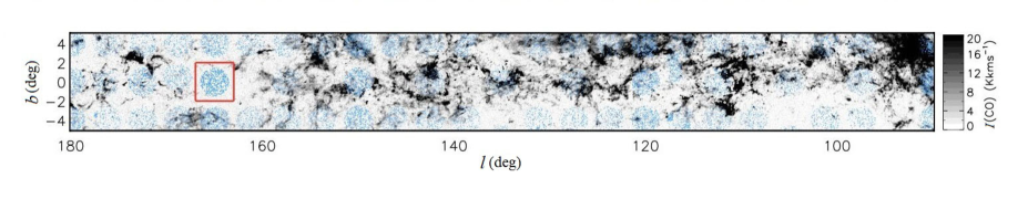
Figure 1: Planck velocity-integrated CO (1–0) emission intensity contours of the Galactic plane region $\mid b\mid\leq 5^{\circ}$. Blue dots: APOGEE giants; red square: selected G$l165^{\circ}\pm 0$ region.

Based on Figure 1, we selected one candidate diffuse region, ‘$l165^{\circ}$,’ centered on ($l=165.0^{\circ},b=0.0^{\circ}$). It covers $4^{\circ}\times 4^{\circ}$ on the sky, and the mean $I$(CO) is about 2 K km s^-1; the region is indicated by the red square. The other two factors, the visual extinction and the dust IR emission intensity, are also used in selecting the diffuse region (see for more details Section 1). The $l165^{\circ}$ region shows essentially very little extinction with $A_{V}\sim 1.0\,{\rm mag}$ in the visual extinction maps of Dobashi et al. (2005) and from Chen et al. (2015). This amount of extinction matches very well the characteristic extinction of diffuse clouds, i.e., the total visual extinction $A_{V}$ is $\sim$0–1 mag (Snow & McCall 2006; Draine 2011). In addition, the Spitzer/MIPS 24$\,{\rm\mu m}$ image shows no detectable 24$\,{\rm\mu m}$ emission for $l165^{\circ}$. Therefore, the CO line intensity, visual extinction, and dust emission all indicate that the $l165^{\circ}$ region is very diffuse.

3 Data and Tracers

The extinction is most reliably determined by comparing spectrophotometry of two stars (one with negligible foreground dust, the other heavily reddened) of the same spectral class under the assumption that the dust extinction decreases to zero at very long wavelengths (Draine 2003). Lutz (1996) probed the extinction law toward the Galactic Center between 2.5 and $19\,{\rm\mu m}$ by comparing the observed and expected intensity ratios of the hydrogen recombination lines. In addition, the color-excess method is widely applied to photometric data; it can probe more deeply than the spectrum-pair method. Hence, most IR extinction studies are performed using the color-excess method. In brief, this statistical method computes the ratio of two color excesses for a group of tracers with homogeneous intrinsic color indices. Red-giant stars (RGs) and RC stars are appropriate tracers. The advantages of using these tracers are that they are bright and numerous, and they can be selected based on near-IR color–magnitude diagrams (CMDs). Their disadvantage is that contamination by other types of stars is unavoidable (Wang & Jiang 2014). Recently, Wang & Jiang (2014) and Xue et al. (2016) adopted a new method that combines photometry and spectroscopy to derive accurate stellar extinction values. In this work, we will follow their method to investigate the optical-to-mid-IR extinction law of the $l165^{\circ}$ diffuse region. In essence, the intrinsic color index is calculated based on the stellar parameters, and the color excess is subsequently derived.

3.1 Data

Broad-band photometric data from APASS, XSTPS-GAC, 2MASS, and WISE are used to derive the observed colors, while the stellar spectroscopic data set from APOGEE is used to determine the intrinsic colors.

3.1.1 Optical to Infrared Photometric Data: APASS, XSTPS-GAC, 2MASS, WISE Surveys

The American Association of Variable Star Observers (AAVSO) Photometric All-Sky Survey (APASS) is conducted in five filters: Landolt $B$ and $V$ and Sloan $g^{\prime},r^{\prime}$, and $i^{\prime}$. The reliable magnitude range in the $V$ band runs from $V=7\,{\rm mag}$ to 17$\,{\rm mag}$ (Henden & Munari 2014). The latest, DR9 catalog contains photometry for approximately 62 million objects, covering about 99% of the sky (Henden et al. 2016). Munari et al. (2014) investigated the external accuracy of APASS photometry, based on secondary Landolt and Sloan photometric standard stars, and on a large body of literature data on field and cluster stars. They confirmed that the APASS photometry did not show any offsets or trends. We obtained the $B$ and $V$ data from the APASS/DR9.

Xuyi 1.04/1.20 m Schmidt Telescope Photometric Survey of the Galactic Anticenter (XSTPS-GAC) consists of two parts, one centered in the Galactic Anticenter area covering $140^{\circ}<l<240^{\circ}$ and $-60^{\circ}<b<40^{\circ}$, the other covering the M31/M33 area (for more details, see Liu et al. 2014; Zhang et al. 2014). The XSTPS-GAC photometric catalog provides $g$-, $r$-, and $i$-band data for more than 100 million stars; the passbands are the same as for the Sloan Digital Sky Survey (SDSS). The limiting magnitude is about 19$\,{\rm mag}$ in the $r$ band ($\sim 10\sigma$), with an astrometric accuracy of $\sim 0.1$ arcsec (Liu et al. 2014). Chen et al. (2014) and Liu et al. (2014) pointed out that flux calibration with respect to the SDSS photometry produces a photometric accuracy of better than 2% for a single frame and $\sim$2–3% for the whole observation area. We take the $g,r$, and $i$ photometric data from the sample of Chen et al. (2014), who used it to determine the three-dimensional extinction map of the Galactic Anticenter.

The Two Micron All Sky Survey (2MASS) is a near-IR ground-based whole-sky survey using two 1.3 m aperture telescopes (Skrutskie et al. 1997). Over 470 million sources in its point-source catalog provide measurements in the $J$, $H$, and ${K_{\rm s}}$ bands.

The Wide-Field Infrared Survey Explorer (WISE) survey is a full-sky mid-IR survey with a 40 cm space-borne telescope (Wright et al. 2010). It mapped the sky in the $W1,W2,W3$, and $W4$ bands (with central wavelengths of, respectively, 3.4, 4.6, 12, and 22$\,{\rm\mu m}$) and yielded a source catalog of over 563 million objects with 5$\sigma$ photometric sensitivities of about 0.068, 0.098, 0.86, and 5.4 mJy in $W1,W2,W3$, and $W4$, respectively, in unconfused regions along the ecliptic plane. Because the sensitivities of the $W3$ and $W4$ bands are relatively low, we only consider the $W1$ and $W2$ bands here. The WISE photometric data are taken from the sample of Chen et al. (2014), who adopted the WISE All-Sky source catalog.

3.1.2 Spectroscopic Data: The SDSS/APOGEE Survey

APOGEE is a near-IR $H$-band (1.51–1.70$\,{\rm\mu m}$), high-resolution ($R\sim 22,500$) spectroscopic survey. Part of SDSS-III DR12, it includes all data obtained from 2008 August to 2014 June (Alam et al. 2015). The APOGEE Stellar Parameter and Chemical Abundances Pipeline (ASPCAP) extracts stellar parameters, including effective temperatures $T_{\rm eff}$, surface gravities $\log g$, and detailed elemental abundances such as metallicities [Fe/H] (Holtzman et al. 2015). The uncertainties are typically 50–100 K in $T_{\rm eff}$, 0.2 dex in $\log g$, and 0.03–0.08 dex in [Fe/H] (Mészáros et al. 2013). It is a good tool to investigate the composition and dynamics of stars in the Galaxy. The APOGEE data release also includes the APOGEE red-clump (APOGEE–RC) catalog from DR11 and DR12. The stellar parameters in the APOGE–RC catalog are based on APOGEE data and calibrated using stellar evolution models and asteroseismology data. RC stars are selected by their position in color–metallicity–surface-gravity–effective-temperature space (Bovy et al. 2014). The APOGEE–RC DR12 catalog contains about 20,000 likely RC stars with an estimated contamination of less than 3.5% (Bovy et al. 2014).

By cross-matching the photometric and spectroscopic catalogs, we have constructed a multiband stellar sample. To summarize, in total ten-band optical-to-IR (i.e., $B,V,g,r,i$, $J$, $H$, ${K_{\rm s}}$, $W1$, and $W2$) photometric data have been collected from the APASS, XSTPS-GAC, 2MASS, and WISE survey programs. The stellar parameters $T_{\rm eff}$, $\log g$, and [Fe/H] were extracted from the APOGEE catalog.

3.2 Tracers

RGs and RC stars are frequently used as IR interstellar extinction tracers. RGs with a small scatter in the IR intrinsic color index ($C_{J{K_{\rm s}}}^{0}$; Gao et al. 2009; Wang et al. 2013) are usually selected based on mid-IR color restrictions: $[3.6]-[4.5]<0.6$ mag and $[5.8]-[8.0]<0.2$ mag (Flaherty et al. 2007). Although these criteria could effectively remove sources with intrinsic IR excesses, some asymptotic giant-branch (AGB) stars that suffer from circumstellar extinction may contaminate the RG sample. RC stars are a group of K2III-type stars in the core-helium-burning stage. Their absolute magnitude is around $M_{K}=-1.61\pm 0.03\,{\rm mag}$ (Alves 2000), and their near-IR intrinsic color index is $0.65\leq C_{J{K_{\rm s}}}^{0}\leq 0.75$ mag (Wainscoat et al., 1992; González-Fernández et al., 2014; Wang & Jiang, 2014). Because of the constant IR luminosity and very small scatter in $J-{K_{\rm s}}$, their distribution in the near-IR $(J-{K_{\rm s}})$ versus ${K_{\rm s}}$ CMD forms a narrow strip, which is commonly adopted to identify RCs. However, the observed $(J-{K_{\rm s}})$ color ($C_{J{K_{\rm s}}}$) depends only on the interstellar extinction, while ${K_{\rm s}}$ magnitudes depend on both interstellar extinction and distance, leading to a large dispersion of RC stars in the CMD. Therefore, selection of RC stars from the CMD may include some dwarf stars, specifically a fraction of $\,{\sim}$ 2.5–5% for ${K_{\rm s}}<12.5\,{\rm mag}$, and up to $\,{\sim}$ 10–40% for $13\,{\rm mag}<{K_{\rm s}}<14\,{\rm mag}$ (López-Corredoira et al., 2002; Cabrera-Lavers et al., 2007). In addition, selection of the RC strip in the CMD is not universal for all sightlines, and it is also somewhat subjective on the basis of empirical and visual inspection.

To avoid these uncertainties and contamination, we obtained a homogeneous RC sample with the current-best available quality from a combination of photometric and spectroscopic data. First, the photometric quality must be $\sigma<0.1$ mag in the $B$ and $V$ bands and $\sigma<0.05$ mag in the $g,r,i,J,H,{K_{\rm s}},W1$, and $W2$ bands. As the metallicity [Fe/H] would affect the intrinsic color at short wavelengths, we limit the [Fe/H] of giants ($\log g\leq 3.0$) to [Fe/H]$>-0.5$ dex. Next, likely RC candidates were selected based on their clumping in the $T_{\rm eff}$–$\log g$ contour map resulting from the entire APOGEE DR12 catalog, in the ranges $4550\,{\rm K}\leq T_{\rm eff}\leq 5050\,{\rm K}$ and $2.3\leq\log g\leq 3.0$. In addition, the selected candidates were cross-matched with the APOGEE–RC catalog. In fact, not all RC candidates are included in the APOGEE–RC catalog. Therefore, our final, homogeneous RC sample contains those RC candidates that are included in the APOGEE–RC catalog. For the diffuse $l165^{\circ}$ region, there are only 18 RC stars with the full ten-band data of high quality. Their names, locations, stellar parameters, and the $B,V$, and $J$-band photometric data are listed in Table 1, sorted by increasing $T_{\rm eff}$.

Table 1: Eighteen RCs in the $l165^{\circ}$ region selected for our extinction study

No.	Name	$l$	$b$	$T_{\rm eff}$	$\log g$	[Fe/H]	$V$	$B-V$	$V-J$
		(∘)	(∘)	(K)			(mag)	(mag)	(mag)
1	2M05114361+4105251	166.05	0.97	4691.40	2.55	0.26	15.45	1.44	2.77
2	2M04564963+4125154	164.09	$-$1.05	4844.28	2.45	$-$0.19	14.61	1.53	2.83
3	2M05113045+4121184	165.82	1.10	4867.70	2.66	$-$0.04	14.60	1.47	2.41
4	2M05103457+4157164	165.23	1.31	4878.76	2.69	$-$0.45	13.99	1.24	2.19
5	2M05063114+4025047	166.01	$-$0.22	4907.07	2.75	0.10	14.45	1.41	2.62
6	2M05104317+4051399	166.13	0.68	4909.86	2.65	$-$0.10	14.19	1.26	2.37
7	2M05072939+4019254	166.19	$-$0.13	4910.46	2.66	$-$0.13	14.21	1.28	2.43
8	2M05014034+4045148	165.18	$-$0.75	4926.30	2.54	$-$0.28	15.11	1.30	2.60
9	2M05113657+4102440	166.08	0.93	4935.57	2.70	$-$0.42	15.42	1.09	2.30
10	2M05055643+4124051	165.16	0.29	4943.94	2.71	$-$0.15	14.36	1.38	2.51
11	2M05081159+4135433	165.25	0.74	4977.03	2.61	$-$0.23	14.48	1.48	2.79
12	2M05041714+4232248	164.06	0.73	4977.43	2.76	$-$0.33	13.95	1.21	2.37
13	2M05070978+4134192	165.16	0.57	4982.41	2.76	$-$0.27	14.25	1.26	2.38
14	2M05111337+4102241	166.04	0.87	4989.09	2.75	$-$0.03	13.77	1.32	2.41
15	2M05031839+4000169	165.96	$-$0.96	4992.78	2.63	$-$0.34	15.82	1.43	3.05
16	2M04592396+4023594	165.19	$-$1.30	4993.97	2.67	$-$0.39	15.14	1.49	2.95
17	2M05000136+4219417	163.75	$-$0.02	5007.93	2.93	$-$0.01	14.68	1.47	2.58
18	2M05102193+4121433	165.68	0.98	5027.16	2.79	$-$0.22	14.39	1.20	2.39

4 Method

We use the color-excess ratio to express the extinction law, where the color excess $E(\lambda_{1}-\lambda_{2})=C_{\lambda_{1}\lambda_{2}}-C_{\lambda_{1}\lambda_{2}}^{0}$ is the difference between the observed color index $C_{\lambda_{1}\lambda_{2}}$ and the intrinsic color index $C_{\lambda_{1}\lambda_{2}}^{0}$. We use $E(V-\lambda_{x})/E(B-V)$ ($\lambda_{x}:B,g,r,i,J,H,{K_{\rm s}},W1,W2$) to represent the interstellar extinction law. The key problem is to determine the intrinsic color index $(V-\lambda_{x})_{0}$. Here, we will introduce two methods to obtain $(V-\lambda_{x})_{0}$.

4.1 Intrinsic Colors

4.1.1 Analytic $T_{\rm eff}$–intrinsic color $C_{\lambda_{1}\lambda_{2}}^{0}$ relation

Wang & Jiang (2014) suggested that the intrinsic color index could be represented by the bluest observed color index under some circumstances for a given $T_{\rm eff}$. This means that the intrinsic color index $C_{\lambda_{1}\lambda_{2}}^{0}$ can be derived from their effective temperatures $T_{\rm eff}$ by considering the bluest star at the same $T_{\rm eff}$ not affected by reddening. They determined the $T_{\rm eff}$–near-IR intrinsic color index relation by means of a quadratic fit to the bluest stars in the $T_{\rm eff}$ vs. observed color index diagram for APOGEE K-type giants ($3500\,{\rm K}\leq T_{\rm eff}\leq 4800\,{\rm K}$). Xue et al. (2016) further applied this method to multiple mid-IR bands for the APOGEE G- and K-type giants ($3600\,{\rm K}\leq T_{\rm eff}\leq 5200\,{\rm K}$). In order to determine the blue envelope in the $T_{\rm eff}$ vs. observed color index diagram, they adopted a mathematical definition for the blue edge. First, they chose the median color of the bluest 5% of stars in bins of $\Delta T_{\rm eff}=100\,{\rm K}$ to represent the unreddened color. Then, they used an exponential or quadratic function to fit the bluest color. The original idea underlying this method was developed by Ducati (2001).

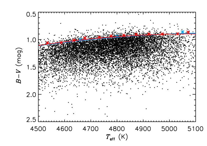
Figure 2: $T_{\rm eff}$ vs. observed color $(B-V)$ diagram. Black dots are the selected K-type giants, red asterisks show the median values of the bluest stars in bins of $\Delta T_{\rm eff}=50\,{\rm K}$. The red solid line denotes the quadratic fit result to these red asterisks. For comparison, the blue line is the quadratic fit result to the discrete intrinsic color data (blue asterisks) of Johnson (1966).

Since RC stars in the range $4550\,{\rm K}\leq T_{\rm eff}\leq 5050\,{\rm K}$ are selected as tracers for investigating the interstellar extinction, we concentrate on the APOGEE K-type giants with $4500\,{\rm K}\leq T_{\rm eff}\leq 5100\,{\rm K}$ to determine the intrinsic colors in the optical bands, since the relation between IR color and $T_{\rm eff}$ has already been derived (Xue et al. 2016). The following constraints are used to obtain a K-giant sample: (1) $4500\,{\rm K}\leq T_{\rm eff}\leq 5100\,{\rm K}$; (2) $\log g\leq 3.0$; (3) photometric uncertainties $\sigma<0.1$ mag in the $B,V$ bands and $\sigma<0.05$ mag in the $g,r,i,J,H,{K_{\rm s}},W1,W2$ bands; (4) observed spectral signal-to-noise ratio $>100$ and difference between the observed and synthetic model spectra $\chi^{2}_{\rm ASPCAP}<30$; (5) [Fe/H] $>-0.5$ dex. Note that this step employs stars from all fields, including from high Galactic latitude areas, and is unbiased as to any specific environment. A series of discrete median effective temperatures $\langle T_{\rm eff}\rangle$ and median observed colors $\langle C_{\lambda_{1}\lambda_{2}}\rangle$ in bins of $\Delta T_{\rm eff}=50\,{\rm K}$ are selected from the bluest 5% of stars. A quadratic function is fitted to this [$\langle T_{\rm eff}\rangle$, $\langle C_{\lambda_{1}\lambda_{2}}\rangle$] series to determine the analytic expression for the $T_{\rm eff}$–intrinsic color relation. Figure 2 is the $T_{\rm eff}$ vs. observed color $(B-V)$ diagram for the K-giant sample (black dots). The red asterisks are the median values for the bluest 5% of stars, and the red line is the quadratic best-fitting result. For comparison, we also plot the quadratic fit result for discrete intrinsic color data (blue asterisks) given by Johnson (1966; blue line). The two lines are highly consistent. The results in other bands are as follows:

$$C^{0}_{\rm BV}=17.10-6.38(\frac{T_{\rm eff}}{10^{3}\,{\rm K}})+0.628(\frac{T_{\rm eff}}{10^{3}\,{\rm K}})^{2}~{}~{},$$ (1)

$$C^{0}_{\rm gV}=11.40-4.31(\frac{T_{\rm eff}}{10^{3}\,{\rm K}})+0.424(\frac{T_{\rm eff}}{10^{3}\,{\rm K}})^{2}~{}~{},$$ (2)

$$C^{0}_{\rm Vr}=12.93-5.03(\frac{T_{\rm eff}}{10^{3}\,{\rm K}})+0.500(\frac{T_{\rm eff}}{10^{3}\,{\rm K}})^{2}~{}~{},$$ (3)

$$C^{0}_{\rm Vi}=21.12-8.20(\frac{T_{\rm eff}}{10^{3}\,{\rm K}})+0.818(\frac{T_{\rm eff}}{10^{3}\,{\rm K}})^{2}~{}~{},$$ (4)

$$C^{0}_{\rm VJ}=23.57-8.50(\frac{T_{\rm eff}}{10^{3}\,{\rm K}})+0.823(\frac{T_{\rm eff}}{10^{3}\,{\rm K}})^{2}~{}~{},$$ (5)

where $C^{0}_{\rm BV}$, $C^{0}_{\rm gV}$, $C^{0}_{\rm Vr}$, $C^{0}_{\rm Vi}$, and $C^{0}_{\rm VJ}$ represent the intrinsic color indices $(B-V)_{0},(g-V)_{0},(V-r)_{0}$, $(V-i)_{0}$, and $(V-J)_{0}$, respectively. Xue et al. (2016) already determined the multi-band intrinsic IR colors for APOGEE G- and K-type giants with $3600\,{\rm K}\leq T_{\rm eff}\leq 5200\,{\rm K}$. Therefore, we adopt the IR intrinsic colors ($J-H)_{0}$, $(J-{K_{\rm s}})_{0}$, $({K_{\rm s}}-W1)_{0}$, and $({K_{\rm s}}-W2)_{0}$ from their work to determine $(V-H)_{0}$, $(V-{K_{\rm s}})_{0}$, $(V-W1)_{0}$, and $(V-W2)_{0}$ (hereafter $C^{0}_{\rm VH}$, $C^{0}_{\rm VK}$, $C^{0}_{\rm VW1}$, and $C^{0}_{\rm VW2}$, respectively).

4.1.2 Padova stellar models

The stellar intrinsic color can be calculated from stellar evolution models once the metallicity, effective temperature, and surface gravity are known. One of the most commonly used stellar evolution models are the Padova isochrone sets of Marigo et al. (2008) with the Girardi et al. (2010) Case A correction for low-mass, low-metallicity AGB tracks. This isochrone set was used to determine extinction maps toward the Milky Way bulge based on APOGEE targets by Schultheis et al. (2014). We adopt very similar procedures: a step of 0.2 dex in metallicity in the range of $-0.5<$[Fe/H]$<0.5$ dex and $\bigtriangleup(\log$ age)=0.05 [Gyr] within the range $6.6\leq\log\rm{age/yr}\leq 10.13$. Specific steps are as follows: (1) according to the stellar [Fe/H], we derive the sequence of isochrones with the closest, constant metallicity for each star; (2) the absolute magnitude is derived from a two-dimensional interpolation in the corresponding $\log g$ vs. $T_{\rm eff}$ plane, rather than based simply on the closest data point. The interpolated value is based on a cubic interpolation of the values of the neighboring grid points for each $\log g$ and $T_{\rm eff}$, and absolute magnitude dimension, respectively. In this way, we derived the absolute magnitudes in ten bands ($B,V,g,r,i,J,H,{K_{\rm s}},W1,W2$) for each RC star, and the intrinsic colors for any pair of bands are thus available.

4.1.3 Comparison

Table 2: Multi-band intrinsic color indices for the 18 RCs in the $l165^{\circ}$ region

No.	$M_{K_{\rm s}}$	$C^{0}_{\rm BV}$	$C^{0}_{\rm gV}$	$C^{0}_{\rm Vr}$	$C^{0}_{\rm Vi}$	$C^{0}_{\rm VJ}$	$C^{0}_{\rm VH}$	$C^{0}_{\rm VK}$	$C^{0}_{\rm VW1}$	$C^{0}_{\rm VW2}$
Analytic results
1	–	0.992	0.505	0.337	0.644	1.81	2.35	2.45	2.52	2.43
2	–	0.932	0.463	0.297	0.582	1.71	2.21	2.30	2.37	2.29
3	–	0.925	0.459	0.293	0.576	1.70	2.19	2.28	2.35	2.27
4	–	0.922	0.457	0.291	0.573	1.70	2.19	2.27	2.34	2.26
5	–	0.916	0.452	0.287	0.568	1.68	2.17	2.25	2.32	2.24
6	–	0.915	0.452	0.287	0.567	1.68	2.16	2.25	2.32	2.24
7	–	0.915	0.451	0.287	0.567	1.68	2.16	2.25	2.32	2.24
8	–	0.912	0.449	0.285	0.565	1.68	2.15	2.24	2.31	2.23
9	–	0.910	0.448	0.284	0.563	1.67	2.15	2.23	2.30	2.22
10	–	0.908	0.447	0.283	0.562	1.67	2.14	2.22	2.30	2.22
11	–	0.903	0.443	0.281	0.559	1.66	2.12	2.20	2.28	2.20
12	–	0.903	0.443	0.281	0.559	1.66	2.12	2.20	2.28	2.20
13	–	0.903	0.443	0.281	0.559	1.66	2.12	2.20	2.27	2.20
14	–	0.902	0.442	0.280	0.559	1.65	2.12	2.20	2.27	2.19
15	–	0.901	0.442	0.280	0.559	1.65	2.12	2.19	2.27	2.19
16	–	0.901	0.442	0.280	0.559	1.65	2.11	2.19	2.27	2.19
17	–	0.900	0.441	0.280	0.558	1.65	2.11	2.19	2.26	2.18
18	–	0.898	0.440	0.279	0.558	1.64	2.10	2.18	2.25	2.18
Model results
1	$-$2.17	1.14	0.59	0.32	0.58	1.85	2.39	2.48	2.52	2.44
2	$-$2.40	1.01	0.51	0.26	0.50	1.71	2.23	2.30	2.34	2.28
3	$-$1.83	1.01	0.52	0.27	0.50	1.70	2.20	2.28	2.32	2.25
4	$-$0.97	0.95	0.48	0.25	0.48	1.68	2.20	2.27	2.31	2.26
5	$-$1.74	1.01	0.52	0.27	0.49	1.68	2.17	2.25	2.28	2.21
6	–	–	–	–	–	–	–	–	–	–
7	$-$1.81	0.98	0.5	0.26	0.48	1.67	2.16	2.24	2.27	2.21
8	$-$2.18	0.95	0.48	0.25	0.48	1.66	2.15	2.23	2.26	2.2
9	$-$1.19	0.92	0.47	0.24	0.46	1.64	2.14	2.21	2.24	2.2
10	–	–	–	–	–	–	–	–	–	–
11	$-$2.00	0.94	0.47	0.24	0.46	1.62	2.10	2.17	2.2	2.15
12	$-$1.34	0.92	0.46	0.24	0.46	1.62	2.11	2.18	2.21	2.16
13	$-$1.41	0.93	0.47	0.24	0.46	1.62	2.10	2.17	2.20	2.15
14	$-$1.74	0.96	0.49	0.25	0.46	1.61	2.09	2.16	2.19	2.13
15	$-$1.80	0.92	0.46	0.23	0.45	1.60	2.08	2.15	2.18	2.14
16	$-$1.65	0.91	0.46	0.23	0.45	1.60	2.09	2.15	2.18	2.14
17	$-$1.11	0.96	0.49	0.24	0.45	1.61	2.08	2.15	2.19	2.13
18	$-$1.48	0.91	0.46	0.24	0.45	1.59	2.06	2.13	2.16	2.11

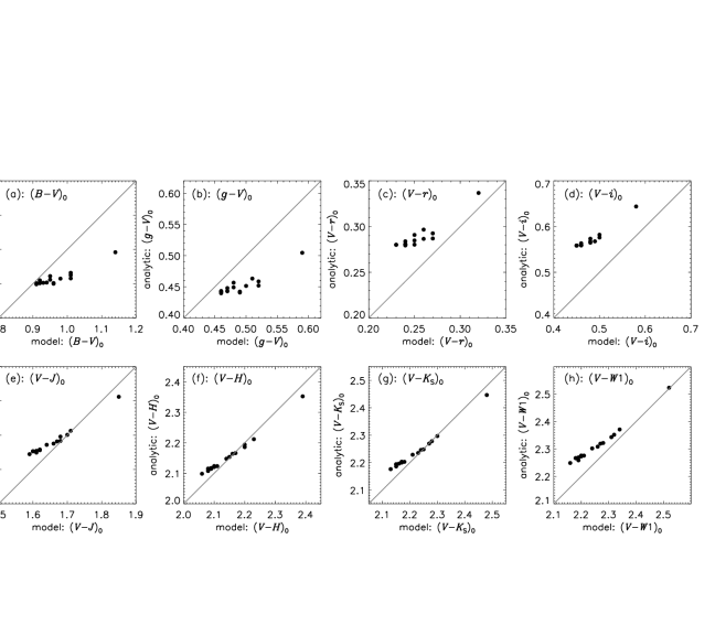
Figure 3: Comparison of the 18 RC intrinsic color indices derived from the analytic $T_{\rm eff}$–$C_{\lambda 1\lambda 2}^{0}$ relation with those derived from the Padova isochrone models. The values are listed in Table 2.

The intrinsic color indices of the 18 RC stars in the $l165^{\circ}$ region are included in Table 2. The top part displays the intrinsic values derived from the analytic $T_{\rm eff}$–$C_{\lambda 1\lambda 2}^{0}$ relation; the bottom part displays the values derived from the Padova stellar models. The ${K_{\rm s}}$-band absolute magnitudes from the Padova stellar models are also listed in the first column of Table 2. They range from ${K_{\rm s}}=-0.97\,{\rm mag}$ to $-2.40\,{\rm mag}$. The average ${K_{\rm s}}$-band absolute magnitude value, ${K_{\rm s}}=-1.68\,{\rm mag}$, is slighter smaller than the typical RC value, $-1.54\,{\rm mag}$ – $-1.61\,{\rm mag}$, which results in a higher extinction value. We also compare the intrinsic color indices determined based on these two methods. Figure 3 shows the comparison. The vertical axis shows the intrinsic color indices derived from the analytic $T_{\rm eff}$–$C_{\lambda 1\lambda 2}^{0}$ relation, and the horizontal axis shows the values derived from the Padova models. The intrinsic IR color indices, i.e., $C^{0}_{\rm VJ}$, $C^{0}_{\rm VH}$, $C^{0}_{\rm VK}$, and $C^{0}_{\rm VW1}$, are internally consistent. However, Figure 3 shows that the optical color indices exhibit notable differences: for $C^{0}_{\rm BV}$ and $C^{0}_{\rm gV}$, the analytic results are lower than the model results; for $C^{0}_{\rm Vr}$ and $C^{0}_{\rm Vi}$, the analytic results are higher than the model results. It is unclear whether these differences are caused by flaws in the stellar models or by the analytic method. Nevertheless, the difference is mostly smaller than 0.05 $\,{\rm mag}$ in color, comparable to the photometric uncertainties.

4.2 Color-Excess Ratio

With the observed color index (the difference between two observed magnitudes) and the intrinsic color index (derived from its dependence on $T_{\rm eff}$ or on isochrone sets), the color excess can be calculated easily. The color excesses $E(V-\lambda_{x})$ ($\lambda_{x}:B,g,r,i,J,H,{K_{\rm s}},W1,W2$) were derived for each sample star. In principle, the color-excess ratio, e.g., $E(V-\lambda_{x})/E(B-V)$, can be regarded as indicator of the extinction law.

5 Results and Discussion

5.1 Optical–Mid-IR Extinction

Table 3: Multi-band color-excess ratios for the 18 RC stars in the $l165^{\circ}$ region

No.	$E_{\rm BV}$	$E_{\rm gV}/E_{\rm BV}$	$E_{\rm Vr}/E_{\rm BV}$	$E_{\rm Vi}/E_{\rm BV}$	$E_{\rm VJ}/E_{\rm BV}$	$E_{\rm VH}/E_{\rm BV}$	$E_{\rm VK_{S}}/E_{\rm BV}$	$E_{\rm VW1}/E_{\rm BV}$	$E_{\rm VW2}/E_{\rm BV}$
Analytic results
1	0.448	0.398	0.731	1.22	2.13	2.45	2.62	2.73	2.72
2	0.598	0.599	0.455	0.980	1.87	2.12	2.33	2.44	2.45
3	0.540	0.501	0.314	0.690	1.31	1.59	1.63	1.79	1.78
4	0.319	0.459	0.428	0.952	1.55	1.76	2.02	2.18	2.25
5	0.493	0.441	0.563	1.04	1.91	2.13	2.31	2.44	2.44
6	0.347	0.387	0.692	1.12	1.97	2.28	2.47	2.66	2.67
7	0.362	0.481	0.605	1.03	2.07	2.39	2.66	2.64	2.73
8	0.386	0.583	0.701	1.33	2.40	2.78	3.03	3.21	3.27
9	0.184	0.448	1.309	2.17	3.43	4.16	4.54	4.72	4.78
10	0.476	0.610	0.433	0.942	1.76	2.03	2.22	2.29	2.28
11	0.575	0.554	0.472	0.991	1.96	2.28	2.48	2.59	2.62
12	0.308	0.482	0.716	1.30	2.33	2.62	2.79	3.05	3.07
13	0.361	0.596	0.501	1.01	1.99	2.32	2.58	2.69	2.67
14	0.416	0.636	0.489	0.992	1.81	2.11	2.23	2.35	2.36
15	0.533	0.561	0.650	1.31	2.62	3.03	3.31	3.41	3.49
16	0.586	0.591	0.512	1.08	2.21	2.59	2.75	2.89	2.93
17	0.573	0.572	0.384	0.828	1.62	1.90	2.06	2.15	2.17
18	0.303	0.544	0.698	1.40	2.47	2.90	3.07	3.20	3.25
Model results
1	0.300	0.309	1.15	2.04	3.05	3.54	3.81	4.09	4.03
2	0.520	0.599	0.594	1.29	2.16	2.41	2.68	2.86	2.83
3	0.455	0.460	0.423	0.99	1.56	1.88	1.93	2.19	2.15
4	0.291	0.423	0.609	1.36	1.75	1.88	2.21	2.51	2.47
5	0.399	0.374	0.739	1.48	2.37	2.63	2.85	3.12	3.10
6	–	–	–	–	–	–	–	–	–
7	0.297	0.423	0.828	1.56	2.56	2.93	3.26	3.38	3.42
8	0.348	0.559	0.878	1.72	2.71	3.10	3.38	3.70	3.71
9	0.174	0.348	1.64	2.90	3.81	4.45	4.92	5.36	5.20
10	–	–	–	–	–	–	–	–	–
11	0.538	0.542	0.580	1.24	2.17	2.48	2.71	2.91	2.89
12	0.291	0.452	0.897	1.72	2.59	2.82	3.03	3.45	3.38
13	0.334	0.563	0.664	1.38	2.26	2.57	2.88	3.13	3.02
14	0.358	0.606	0.653	1.43	2.23	2.53	2.70	2.96	2.92
15	0.514	0.546	0.771	1.57	2.82	3.21	3.52	3.70	3.72
16	0.577	0.569	0.606	1.28	2.34	2.67	2.87	3.08	3.07
17	0.513	0.543	0.506	1.14	1.88	2.18	2.37	2.54	2.53
18	0.291	0.496	0.861	1.83	2.75	3.15	3.35	3.64	3.60

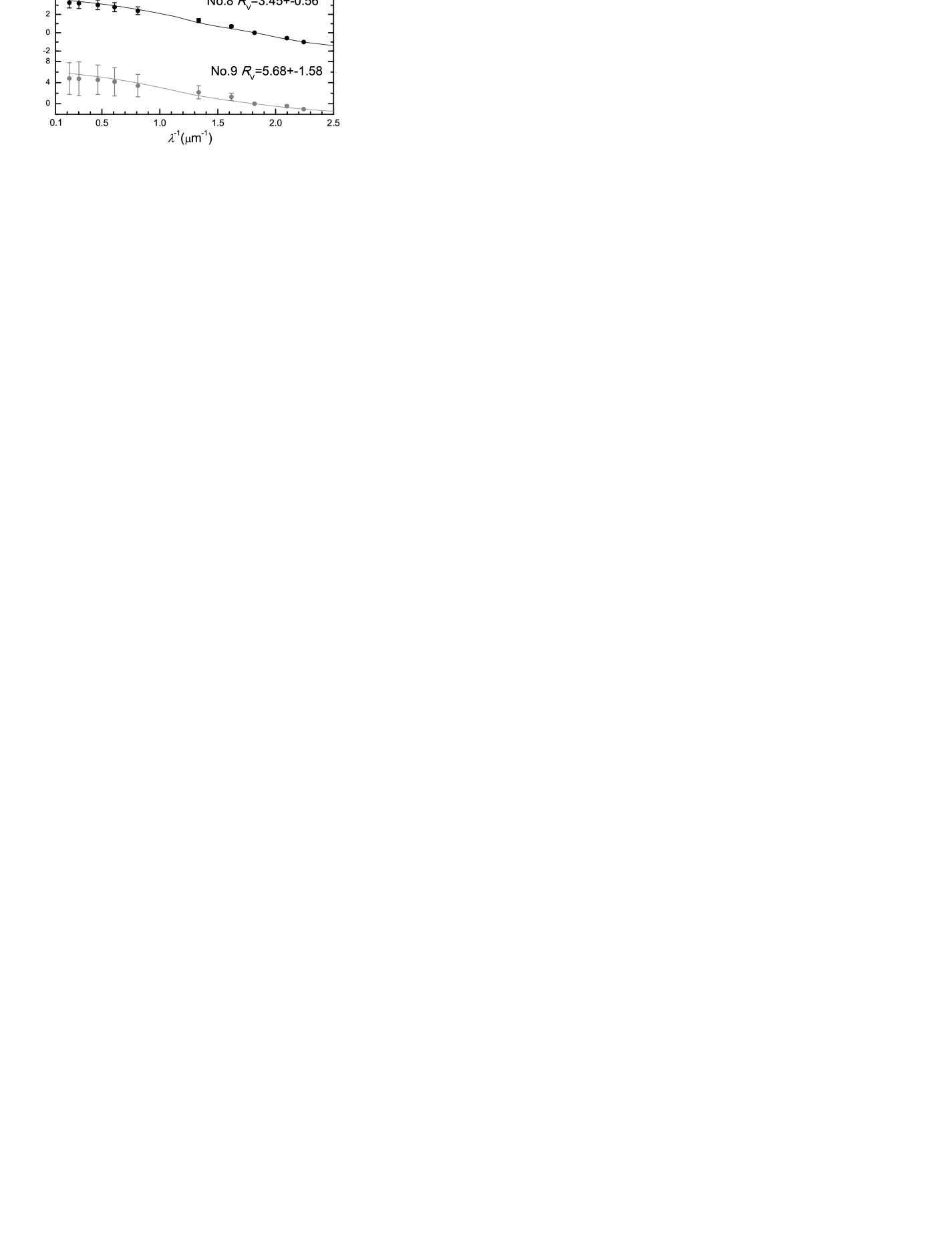
Figure 4: Multi-band extinction and corresponding $R_{V}$ values for the 18 RC stars. Color excesses have been determined by adopting intrinsic colors based on the analytic $T_{\rm eff}$–$C_{\lambda 1\lambda 2}^{0}$ relation. The black line shows the best-fitting results based on using CCM89’s equations. The error bar associated with the $R_{V}$ values were derived based on 20,000 Monte Carlo simulations.

Using the method described above, the color-excess ratios $E(V-\lambda_{x})/E(B-V)$ were derived for the 18 RC stars in the $l165^{\circ}$ region. The results are tabulated in Table 3. Figure 4 displays the variations in the color-excess ratios with waveband, where the color-excess ratios were derived from the analytic $T_{\rm eff}$–$C_{\lambda 1\lambda 2}^{0}$ relation.

The derived extinction law is fitted with the CCM89 equations. Since CCM89 suggested that the extinction law can be described by $R_{V}$, this yields the best-fitting $R_{V}$ value for the prevailing extinction law. In practice, steps of 0.001 are adopted for $0.5\leq R_{V}\leq 7.0$. For each $R_{V}$, $A_{\lambda_{x}}/A_{V}$ is calculated based on the CCM89 equations in all ten bands, from which the color-excess ratio $E(V-\lambda_{x})/E(B-V)$ is derived. The best-fitting $R_{V}$ is determined by assessment of the minimum chi-squared value between the color-excess ratio derived using the CCM89 equations and this work.

The $R_{V}$ values and best-fitting CCM89 lines are shown in Figure 4. The CCM89 extinction curve can fit all cases. Table 3 shows that the $E_{\rm BV}$ and $E_{\rm gV}$ of RC star No. 9 are rather small and the color-excess ratios $E_{\rm V\lambda_{x}}/E_{\rm BV}$ in the $r,i,J,H,{K_{\rm s}},W1$, and $W2$ bands are all apparently larger than the values for the other 17 RC stars. This is caused by the extremely small $E_{\rm BV}$ value, which may be owing to unreliable calibrations in the $B,V$, and $g$ bands. This star was removed from further analysis.

The mean $R_{V}$ value of the remaining 17 RCs is 2.8, which is close to $R_{V}=3.1$, commonly adopted for the average extinction law toward Galactic diffuse clouds. Schlafly & Finkbeiner (2011) measured reddening values for the diffuse ISM based on a large sample of SDSS sources, and found an average extinction law consistent with $R_{V}=3.1$. On the other hand, as can be seen from Figure 4, there is a clear diversity of $R_{V}$ values among stars even in such a small region, which was carefully selected to be very diffuse along any of its sightlines. The lowest $R_{V}$ value is $R_{V}=1.72$ (No. 3); the highest value reaches $R_{V}=3.79$ (No. 15). This diversity significantly exceeds the intrinsic errors (see the next section), and so it is likely real. Moreover, the lowest value of $R_{V}=1.72$ is smaller than the previously published lowest value of $R_{V}=2.1$ towards the HD 210101 sightline. The reddening towards Type Ia supernovae commonly shows a low $R_{V}$ value $<$ 2.0 (Howell 2011, and references therein), in some cases smaller than 1.0, which means the possibility for $R_{V}$ being smaller than 1.7. If we search in larger sample sizes, even lower $R_{V}$ values may be found in the Milky Way. As for the IR bands, there is little variation in $E(J-H)/E(J-{K_{\rm s}})$, with a mean around 0.64, which agrees with the result of Wang & Jiang (2014). The $W1$ and $W2$ bands seem to show some diversity, but with less confidence because of their low sensitivity.

5.2 Error Analysis

The error in the color-excess ratios $[E(V-\lambda_{x})/E(B-V)]_{\rm err}$ originates from a few contributors, including the observed and intrinsic color indices. By constraining the photometric quality of our sample stars to $\sigma<0.1$ mag in the $B,V$ bands and $\sigma<0.05$ mag in the $g,r,i,J,H,{K_{\rm s}},W1$, and $W2$ bands, the average photometric error is $\sim$ 0.06 mag in $B$, $\sim$ 0.04 mag in $V$, and $\sim$ 0.02 mag in $g,r,i,J,H,{K_{\rm s}},W1$, and $W2$ . Consequently, the average error in the observed color index is $\sim$ 0.1 mag for $C_{\rm BV}$ and $\sim$ 0.06 mag for $C_{\rm gV}$, $C_{\rm Vr}$, $C_{\rm Vi}$, $C_{\rm VJ}$, $C_{\rm VH}$, $C_{\rm VK_{S}}$, $C_{\rm K_{S}W1}$, and $C_{\rm K_{S}W2}$. The average error in the APOGEE $T_{\rm eff}$ is $\sim 50\,{\rm K}$. Using the $T_{\rm eff}$—intrinsic color index relation to derive the intrinsic colors from Eqs (1)–(6), the $T_{\rm eff}$ error causes an average error of $\sim$ 0.006 mag for $C^{0}_{\rm BV}$, $\sim$ 0.004 mag for $C^{0}_{\rm gV}$, $\sim$ 0.003 mag for $C^{0}_{\rm Vr}$, $\sim$ 0.004 mag for $C^{0}_{\rm Vi}$, $\sim$ 0.013 mag for $C^{0}_{\rm VJ}$, $\sim$ 0.022 mag for $C^{0}_{\rm VH}$, $\sim$ 0.023 mag for $C^{0}_{\rm VK}$, $\sim$ 0.023 mag for $C^{0}_{\rm VW1}$, and $\sim$ 0.025 mag for $C^{0}_{\rm VW2}$. Combining the photometric and intrinsic color errors, the uncertainties in the color excesses are $(E_{\rm BV})_{\rm err}\sim 0.11$ mag, $(E_{\rm gV})_{\rm err}\sim 0.064$ mag, $(E_{\rm Vr})_{\rm err}\sim 0.063$ mag, $(E_{\rm Vi})_{\rm err}\sim 0.064$ mag, $(E_{\rm VJ})_{\rm err}\sim 0.073$ mag, $(E_{\rm VH})_{\rm err}\sim 0.082$ mag, $(E_{\rm VK_{S}})_{\rm err}\sim 0.083$ mag, $(E_{\rm VW1})_{\rm err}\sim 0.083$ mag, and $(E_{\rm VW2})_{\rm err}\sim 0.085$ mag.

Having thus determined the errors in the color excesses, we use Monte Carlo simulations to calculate the statistical uncertainties in the color-excess ratios $[E(V-\lambda_{x})/E(B-V)]_{\rm err}$ and in the total-to-selective ratio $(R_{V})_{\rm err}$. Taking the error in the color excess into account, we performed 20,000 simulations. A Gaussian function was used to fit the distributions of $E(V-\lambda_{x})/E(B-V)$ and $R_{V}$. The widths of the Gaussian distributions were considered to represent the errors in the color-excess ratios $[E(V-\lambda_{x})/E(B-V)]_{\rm err}$ and the error in the reddening $(R_{V})_{\rm err}$.

The distributions of $E(V-J)/E(B-V)$ and $R_{V}$ resulting from the Monte Carlo resampling for RC star No. 1 are shown in Figure 5 as an example. The distributions of $E(V-J)/E(B-V)$ and $R_{V}$ are both well-fitted by a Gaussian function, with a peak at 2.13 and a width of 0.07, and with a peak at 3.19 and a width of 0.10, respectively. In comparison, our best-fitting results $E(V-J)/E(B-V)=2.13$ and $R_{V}=3.20$ are highly consistent with the Monte Carlo simulation results. The Monte Carlo method reconfirms our fits. The results of our error analysis for the 18 RC stars are presented in Table 4. Except for RC star No. 9, the average error in $R_{V}$ is about 13.4%. In comparison, the range of the derived $R_{V}$ values, from 1.7 to 3.8, is much larger than the typical error, and thus the variation in $R_{V}$ is real and cannot be attributed merely to errors.

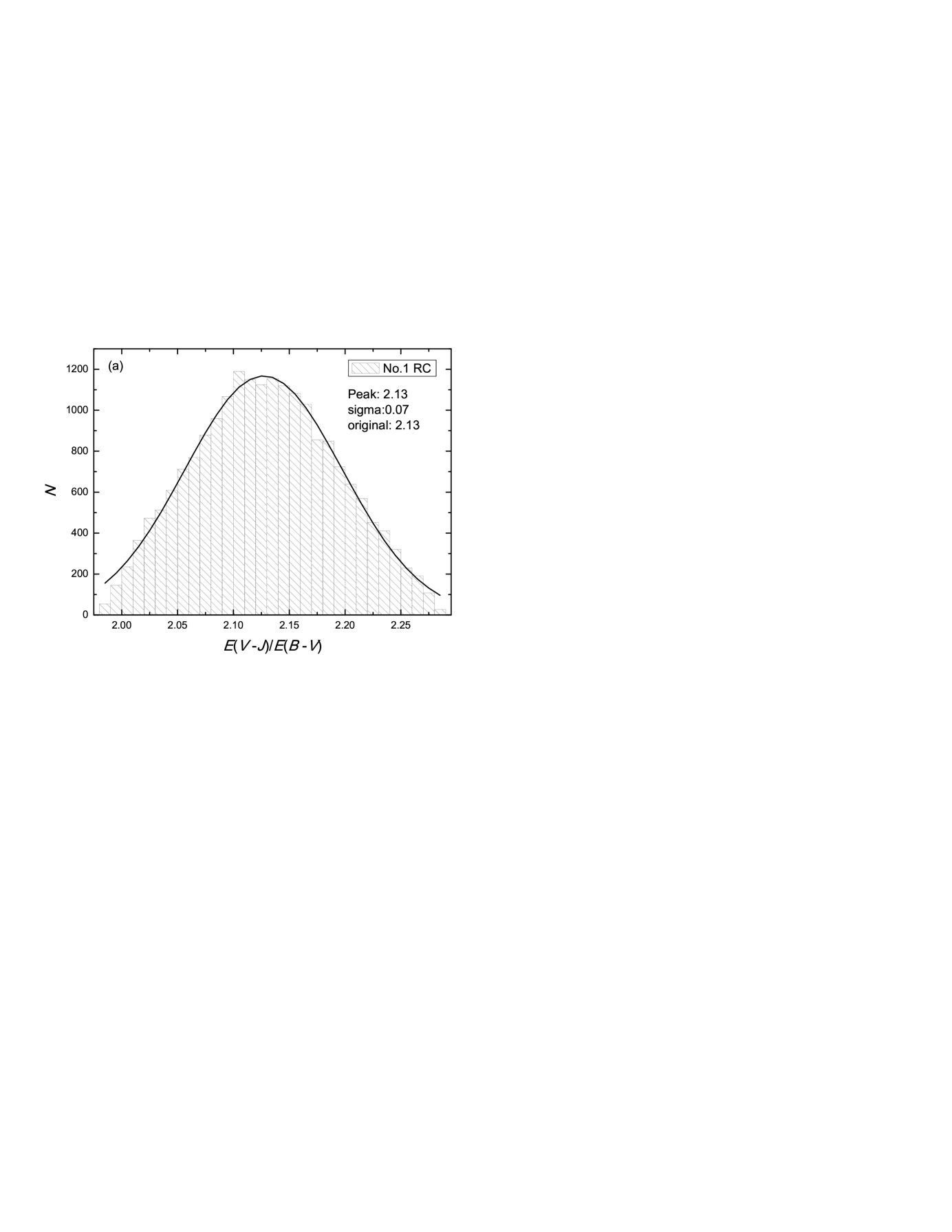
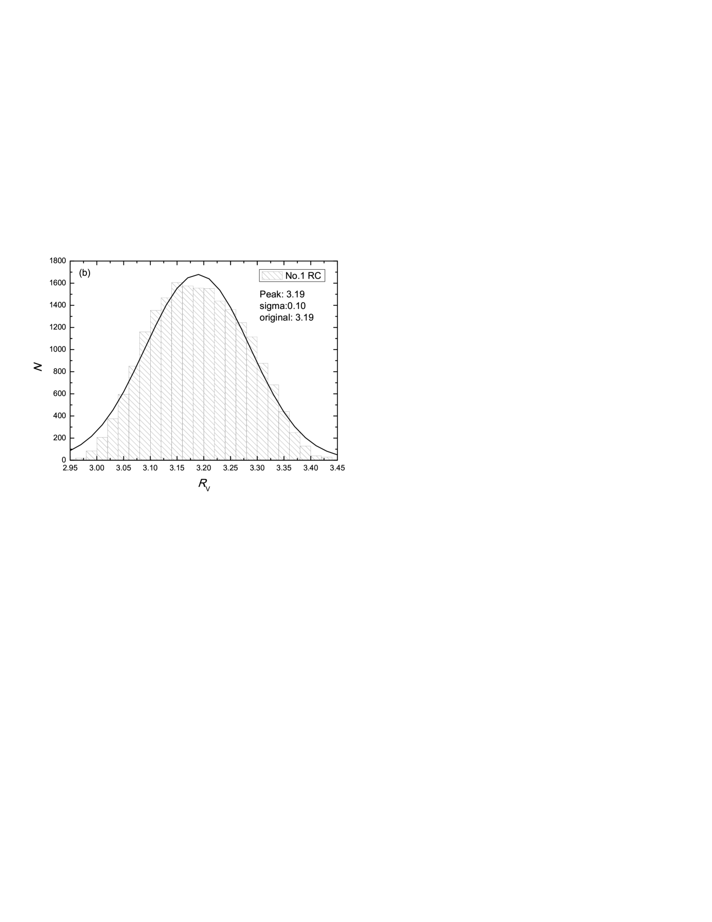
Figure 5: (a) Color-excess ratio $E_{\rm VJ}/E_{\rm BV}$ distribution and (b) reddening $R_{V}$ distributions of 20,000 Monte Carlo resampling results for RC star No. 1.

Table 4: Results of our error analysis for the 18 RC stars in the $l165^{\circ}$ region

No.	1	2	3	4	5	6	7	8	9	10	11	12	13	14	15	16	17	18
$R_{V}$	3.19	2.47	1.72	2.18	2.68	2.97	2.98	3.45	5.68	2.41	2.77	3.45	2.90	2.52	3.79	3.11	2.25	3.75
$(R_{V})_{\rm err}$	0.10	0.20	0.16	0.29	0.23	0.54	0.34	0.56	1.58	0.28	0.20	0.88	0.44	0.38	0.33	0.36	0.24	0.95
Peak($R_{V}$)	3.19	2.47	1.74	2.17	2.68	2.90	2.95	3.41	5.10	2.31	2.68	3.22	2.71	2.37	3.73	2.99	2.15	3.36

5.3 Distances to the RC stars

Variations in $R_{V}$ are usually related to the interstellar environment, whether diffuse or dense. Although the sightlines in the $l165^{\circ}$ region are essentially diffuse, the extinction law still exhibits significant variations. A possible reason may be that the degree of diffusivity varies along different sightlines. In order to quantify the interstellar environment, we derived the distances to the sample stars so that the specific extinction per kiloparsec (kpc) can be measured.

Figure 6: Distribution of reddening $R_{V}$ with (a) color excess $E_{\rm BV}$ and (b) specific visual extinction per kiloparsec $A_{V}/d$ for the 17 RC stars in the $l165^{\circ}$ region.

RC stars are good standard candles for estimating astronomical distances, since their absolute luminosities are fairly independent of stellar composition or age. In particular, the near-IR $I$- and ${K_{\rm s}}$-band luminosities have been widely used to retrieve RC distances. Alves (2000) was the first to consider using the RC ${K_{\rm s}}$-band magnitude as a distance indicator. He found $M_{{K_{\rm s}}}=-1.61\pm 0.03\,{\rm mag}$, with a weak dependence on metallicity. Groenewegen (2008) reinvestigated the absolute magnitude of the RC stars based on revised Hipparcos parallaxes. He obtained $M_{{K_{\rm s}}}=-1.54\pm 0.04\,{\rm mag}$, which is slightly fainter than previously published values. In addition, Nishiyama et al. (2006) used $M_{{K_{\rm s}}}=-1.59\,{\rm mag}$ based on Bonatto et al. (2004) to measure the distance to the Galactic Center. The distance to the Galactic Center measured this way is in agreement with results obtained based on other methods (e.g., de Grijs & Bono 2016). Therefore, we adopt $M_{{K_{\rm s}}}=-1.59\,{\rm mag}$ to estimate the distances to our RC stars.

In order to calculate the distance $d$ using $\log d=1+0.2(m_{K_{\rm s}}-M_{K_{\rm s}}-A_{K_{\rm s}})$, we need to know $A_{K_{\rm s}}$, the ${K_{\rm s}}$-band extinction. As we have derived a series of color excesses $E(V-\lambda_{x})$ and the relative extinction $A_{\lambda_{x}}/A_{V}$ using CCM89’s equations, a series of corresponding $A_{V}$ values can be obtained: $A_{V}=E(V-\lambda_{x})/(1-A_{\lambda_{x}}/A_{V})$. The median $\langle A_{V}\rangle$ of this series is taken as the absolute $V$-band extinction. Then, $A_{\rm K_{S}}=A_{\rm K_{S}}/A_{V}\times\langle A_{V}\rangle$ is obtained. The derived distances range from 2.67 kpc to 4.49 kpc. The average $A_{V}$ per kiloparsec is 0.37 mag kpc^-1, based on taking all 17 RC stars in this region. Considering that the average rate of interstellar extinction in the $V$ band is usually taken as 0.7–1.0 mag kpc^-1, simply based on observations in the solar neighborhood (Gottlieb & Upson 1969; Milne & Aller 1980), a gradient of 0.37 mag kpc^-1 means that we are dealing with a really diffuse medium. The highest specific extinction in our region of interest is approximately 0.56 mag kpc^-1, still significantly below the average rate.

Since the color excess $E(B-V)$ represents in general the density of dust, larger $R_{V}$ is expected at larger $E(B-V)$, like dense clouds usually show high $R_{V}$ values. We investigate the variation in $R_{V}$ with $E(B-V)$ shown in Figure 6a. The Pearson correlation coefficient is $-0.34$, indicating no correlation between $R_{V}$ and $E(B-V)$ in the $E(B-V)$ range from 0.2 to 0.6 mag. Schlafly et al. (2016) measured optical–IR extinction curve spatial variations to tens of thousands of APOGEE stars. They also found that the variation in $R_{V}$ is uncorrelated with dust column density up to $E(B-V)\approx 2$ mag. This non-correlation seems to contradict with normal expectation. However, dense molecular clouds exhibit high dust extinction with $A_{V}>$ 5–10 mag (Snow & McCall 2006), corresponding to $E(B-V)$ $>1.6$ mag (for $R_{V}=3.1$). Therefore, these RC sightlines are still diffuse regions. Dense regions are needed to investigate a possible correlation between $R_{V}$ and $E(B-V)$. On the other hand, a large E(B-V) may result from a pile of diffuse clouds. The specific extinction per distance would be a better measure of the ISM environment. Figure 6b displays the variation in $R_{V}$ with specific visual extinction per kpc, $A_{V}/d$. The error bars were determined using error-propagation theory and based on Monte Carlo simulations. Since the Pearson correlation coefficient between $R_{V}$ and $A_{V}/d$ is 0.14, There is no apparent trend for $R_{V}$ with $A_{V}/d$. If we were to adopt different $M_{{K_{\rm s}}}$ values, $M_{{K_{\rm s}}}$ = $-1.54\,{\rm mag}$ or $-1.61\,{\rm mag}$, the distance would change by about 3%, but this change is systematic and would therefore not change our conclusion, i.e., that the variation in $R_{V}$ is independent of both $E(B-V)$ and $A_{V}/d$ within this small range of $E(B-V)(<0.6)$ mag.

5.4 Effects of Metallicity

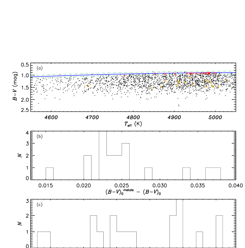
Figure 7: Effects of metallicity on intrinsic RC colors. (a) Similar stars to the 18 target RC stars in the effective temperature $T_{\rm eff}$ vs. observed color index ($B-V$) diagram. The red asterisks are the average values for stars that are similar to each of the 18 target RC stars (yellow asterisks) in $l165^{\circ}$; the blue solid line denotes the $T_{\rm eff}$–$C^{0}_{\rm BV}$ relation, with the green dashed line representing the 1$\sigma$ envelope. (b) Comparison of the intrinsic colors derived above with those determined from the $T_{\rm eff}$–$C^{0}_{\rm BV}$ intrinsic color relation. (c) Comparison of the $R_{V}$ values determined from the intrinsic color indices derived above and those derived from the $T_{\rm eff}$–intrinsic color relation.

The extinction toward the $l165^{\circ}$ region is relatively small, with $A_{V}$ ranging from about 0.7 to 2.0 mag, i.e., $E(B-V)$ ranges from about 0.2 to 0.6 mag. For such a low extinction, a small variation in color excess would lead to a significant difference in the color-excess ratio $E(V-\lambda_{x})/E(B-V)$. Metallicity is a secondary parameter affecting the intrinsic color index, in addition to the effective temperature. In our derivation of the intrinsic colors (Section 4.1.1), metallicity was not taken into account. Therefore, here we discuss the effect of metallicity on the intrinsic colors of RC stars. For each of the 18 target RC stars, stars were selected that have similar stellar parameters (including metallicities) to the target stars and are located ‘close to’ the analytic best-fitting $T_{\rm eff}$–$C^{0}_{\rm BV}$ intrinsic color line. Instead of reading the intrinsic color index from the best-fitting line, the average values of the observed color indices of these similar stars were taken as the intrinsic color indices for each target RC star. The ‘similar’ stellar parameters are defined as those parameters that are found within the ranges $T_{\rm eff}(\rm target)\pm 100\,{\rm K}$, $\log g(\rm target)\pm 0.2$, and $[Fe/H](\rm target)\pm 0.4$ dex. The ‘close’ distance is defined in the sense that the star deviates from the best-fitting $T_{\rm eff}$–$C^{0}_{\rm BV}$ line by less than the uncertainty of 0.06 $\,{\rm mag}$ in the observed color index $(C_{\rm BV})_{\rm err}$. These stars are considered reddening-free, since the deviation from the line of intrinsic color is not larger than the photometric uncertainty. Therefore, the observed color indices of these stars can represent the intrinsic colors. This method was used by Yuan et al. (2013) to derive the empirical extinction law.

Fig 7a exhibits the results for the similar stars selected for the 18 target RC stars in the effective temperature $T_{\rm eff}$ vs. observed color index ($B-V$) diagram. The yellow asterisks represent the 18 target RC stars in the $l165^{\circ}$ region, the blue solid line denotes the $T_{\rm eff}$–$C^{0}_{\rm BV}$ relation, with the cyan dashed line representing the 1$\sigma$ envelope. The red asterisks are the average observed color index values $[C_{\rm BV}]$ of the similar stars, and these average values turn out to be the intrinsic color indices of the 18 RC stars. This method is affected by a systematic bias, as shown in Figure 7a: all reference stars lie below the best-fitting line, which means that they suffer from some extinction. Consequently, the derived $(B-V)_{0}^{\rm metals}$ is redder than the $(B-V)_{0}$ from the $T_{\rm eff}$–$C^{0}_{\rm BV}$ relation, as shown in Figure 7b. Except for $C^{0}_{\rm gV}$, this method results in redder intrinsic color indices $(V-\lambda_{x})_{0}$ in the $r,i,J,H,{K_{\rm s}},W1$, and $W2$ bands. The corresponding color excesses $E(B-V)$ and $E(V-\lambda_{x})$ become smaller, and $E(g-V)$ becomes larger. We also investigated the effect on the $R_{V}$ value. The slightly different intrinsic color indices cause the $R_{V}$ value to become smaller, as shown in Figure 7c: $-0.42<(R_{V})_{\rm metals}-(R_{V})_{0}<-0.14$, while the diversity is still there.

6 Summary

The optical-to-mid-IR extinction law has been derived for the diffuse $l165^{\circ}$ region in the two APASS bands ($B,V$), the three XSTPS-GAC bands ($g,r,i$), the three 2MASS bands ($J,H,{K_{\rm s}}$), and the two WISE bands ($W1,W2$) using RC stars as extinction tracers. Specifically, 18 RC stars in this region were selected from the APOGEE–RC catalog based on their stellar parameters $T_{\rm eff}$, $\log g$, and [Fe/H]. The major results of this paper are as follows:

1. The stellar intrinsic colors were determined for RC stars with effective temperatures in the range $4500\,{\rm K}\leq T_{\rm eff}\leq 5100\,{\rm K}$. Two methods were adopted, one is based on the analytic $T_{\rm eff}$–intrinsic color relation, the other uses Padova isochrone models. The IR intrinsic color indices are consistent with each other. Although the optical color indices exhibit notable differences, the differences in color are mostly smaller than 0.05 $\,{\rm mag}$, comparable to the photometric uncertainties.

2. The extinction curves were derived toward sightlines of 18 RC stars in the diffuse region around $l=165^{\circ}$. The corresponding $R_{V}$ values are determined by fitting the extinction curves with the CCM89 law. The mean $R_{V}$ value of 2.8 is consistent with the commonly adopted value for Galactic diffuse clouds ($R_{V}=3.1$). However, the $R_{V}$ values ranging from 1.7 to 3.8 suggest that the optical extinction law exhibits significant diversity in the $l=165^{\circ}$ region, which is interesting, because it is such a small region (in angular size) of the diffuse ISM. This diversity is beyond the normal expectation that diffuse environments would exhibit an average law with a small variation. Since the extinction law is determined by the dust properties, the result implies that the dust properties are very heterogeneous in their spatial distribution. Consequently, one should be cautious to take an average law to correct for the interstellar extinction. A high spatial resolution study of the extinction law is needed.

3. There is no correlation between $R_{V}$ and $E(B-V)$ in the $E(B-V)$ range of interest, between 0.2 and 0.6 mag. Since these RC sightlines still coincide with the diffuse region, dense regions are needed to investigate any correlation between $R_{V}$ and $E(B-V)$.

4. The distances to our RC sample were derived. They range from 2.67 kpc to 4.49 kpc. The average visual extinction per kiloparsec, $A_{V}/d$ is 0.37 mag kpc^-1, which is lower than the average value for the Milky Way. There is no apparent relation between $R_{V}$ and the specific visual extinction per kpc.

References

- Alam et al. (2015) Alam, S., Albareti, F. D., Allende Prieto, C., et al. 2015, ApJS, 219, 12
- Alves (2000) Alves, D. R. 2000, ApJ, 539, 732
- Bonatto et al. (2004) Bonatto, C., Bica, E., & Girardi, L. 2004, A&A, 415, 571
- Bovy et al. (2014) Bovy, J., Nidever, D. L., Rix, H.-W., et al. 2014, ApJ, 790, 127
- Cabrera-Lavers et al. (2007) Cabrera-Lavers, A., Hammersley, P. L., et al. 2007, A&A, 465, 825
- Cardelli et al. (1989) Cardelli, J. A.,Clayton, G. C., & Mathis, J. S. 1989, ApJ, 345, 245 (CCM89)
- Chen et al. (2014) Chen, B.-Q., Liu, X.-W., Yuan, H.-B., et al. 2014, MNRAS, 443, 1192
- Chen et al. (2015) Chen, B.-Q., Liu, X.-W., Yuan, H.-B., et al. 2015, MNRAS, 448, 2187
- Clark et al. (2012) Clark, J. S., Najarro, F., Negueruela, I., et al. 2012, A&A, 541, 145
- Dame et al. (2001) Dame, T. M., Hartmann, D., & Thaddeus, P. 2001, ApJ, 547, 792
- Deśertet al. (1988) Deśert, F. X., Bazell, D., & Boulanger, F. 1988. ApJ, 334, 815
- de Grijs & Bono (2016) de Grijs, R., & Bono, G. 2016, ApJS, 227, 5
- de Vries & van Dishoeck (1988) de Vries, C. P., & van Dishoeck, E. F. 1988, A&A, 203, 23
- Draine (2003) Draine, B. T. 2003, ARA&A, 41, 241
- Draine (2011) Draine, B. T. 2011, Physics of the Interstellar and Intergalactic Medium (Princeton, NJ: Princeton Univ. Press)
- Dobashi et al. (2005) Dobashi, K., Uehara, H., et al. 2005, PASJ, 57, S1
- Ducati et al. (2001) Ducati, J. R., Bevilacqua, C. M., et al. 2001, ApJ, 558, 309
- Flaherty et al. (2007) Flaherty, K., Pipher, J., Megeath, S., et al. 2007, ApJ, 663, 1069
- Gao et al. (2009) Gao, J., Jiang, B. W., & Li, A. 2009, ApJ, 707, 89
- Girardi & Salaris (2001) Girardi, L., & Salaris, M. 2001, MNRAS, 323, 109
- Girardi et al. (2010) Girardi, L., Williams, B. F., Gilbert, K. M., et al. 2010, ApJ, 724, 1030
- González-Fernández et al. (2014) González-Fernández, C., Asensio Ramos, A., et al. 2014, ApJ, 782, 86
- Gottlieb & Upson (2009) Gottlieb, D., & Upson, W. 1969, ApJ, 157, 611
- Groenewegen (2008) Groenewegen, M. A. T. 2008, A&A, 488, 935
- Henden & Munari (2014) Henden, A., & Munari, U. 2014, Contrib. Astron. Obs. Skalnate Pleso, 43, 518
- Henden et al. (2016) Henden, A., Templeton, M., Terrell, D., et al. 2016, VizieR Online Data Catalog, II/336
- Hodapp et al. (2004) Hodapp, K. W., Kaiser, N., Aussel, H., et al. 2004, AN, 325, 636
- Holtzman et al. (2015) Holtzman, J. A., Shetrone, M., Johnson, J. A., et al. 2015, AJ, 150, 148
- Howell (2011) Howell, D. A. 2011, NatCo, 2, 350
- Indebetouw et al. (2005) Indebetouw, R., et al. 2005, ApJ, 619, 931
- Jiang et al. (2006) Jiang, B. W., Gao, J., Omont, A., Schuller, F., & Simon, G. 2006, A&A, 446, 551
- Liu et al. (2014) Liu, X.-W., et al., 2014, in Feltzing, S., Zhao, G., Walton, N., & Whitelock, P., eds, Proc. IAU Symp. 298, Setting the Scene for Gaia and LAMOST (Cambridge: Cambridge Univ. Press), p. 310
- Johnson (1966) Johnson, H. L. 1966, ARA&A, 4, 193
- Larson et al. (2000) Larson, K. A., Wolff, M. J., et al. 2000, ApJ, 532, 1021
- López-Corredoira et al. (2002) López-Corredoira, M., Cabrera-Lavers, A., et al. 2002, A&A, 394, 883
- Lutz et al. (1996) Lutz, D., et al. 1996, A&A, 315, L269
- Lutz et al. (1999) Lutz, D. 1999, in The Universe as Seen by ISO, eds P. Cox & M. Kessler (ESA Special Publ., Vol. 427; Noordwijk: ESA), p. 623
- Marigo et al. (2008) Marigo, P., Girardi, L., Bressan, A., et al. 2008, A&A, 482, 883
- Mathis (1990) Mathis, J. S. 1990, ARA&A, 28, 37
- Mészáros et al. (2013) Mészáros, S., Holtzman, J., et al. 2013, AJ, 146, 133
- Milne & Aller (1980) Milne, D. K., & Aller, L. H. 1980, AJ, 85, 17
- Munari et al. (2014) Munari, U., Henden, A., Frigo, A., et al. 2014, AJ, 148, 81
- Nataf et al. (2010) Nataf, D. M., Udalski, A., Gould, A., et al. 2010, ApJ, 721, L28
- Nishiyama et al. (2006) Nishiyama, S., Nagata, T., Kusakabe, N., et al. 2006, ApJ, 638, 839
- Nishiyama et al. (2009) Nishiyama, S., Tamura, M., Hatano, H., et al. 2009, ApJ, 696, 1407
- Planck Collaboration XIII (2014) Planck Collaboration XIII, 2014, A&A, 571, A13
- Sarajedini (1990) Sarajedini, A. 1999, AJ, 118, 2321
- Schlafly & Finkbeiner (2011) Schlafly, E. F., & Finkbeiner, D. P. 2011, ApJ, 737, 103
- Schlafly et al. (2016) Schlafly, E. F., Meisner, A. M., Stutz, A. M., et al. 2016, ApJ, 821, 78
- Schultheis et al. (2014) Schultheis, M., Zasowski, G., et al. 2014, AJ, 148, 24
- Skrutskie et al. (1997) Skrutskie, M. F., et al., 1997, in Garzon, F., Epchtein, N., Omont, A., Burton, B., & Persi, P., eds, Astrophys. Space Sci. Libr., 210, The Impact of Large Scale Near-IR Sky Surveys (Dordrecht: Kluwer), p. 25
- Skrutskie et al. (2006) Skrutskie, M. F., et al. 2006, AJ, 131, 1163
- Snow & McCall (2006) Snow, T. P., & McCall, B. J. 2006, ARA&A, 44, 367
- Torres et al. (1991) Torres-Dodgen, A. V., Carroll, M., & Tapia, M. 1991, MNRAS, 249, 1
- Wainscoat et al. (1992) Wainscoat, R., Cohen, M., Volk, K., et al. 1992, ApJS, 83, 146
- Wang et al. (2013) Wang, S., Gao, J., Jiang, B. W., Li, A., & Chen, Y. 2013, ApJ, 773, 30
- Wang & Jiang (2014) Wang, S., & Jiang, B. W. 2014, ApJ, 788, L12
- Welty & Fowler (1992) Welty, D. E., & Fowler, J. R. 1992, ApJ, 393, 193
- Wright et al. (2010) Wright, E. L. et al. 2010, AJ, 140, 1868
- Xue et al. (2016) Xue, M., Jiang, B. W., Gao, J., et al. 2016, ApJS, 224, 23
- Yuan et al. (2013) Yuan, H. B., Liu, X. W., & Xiang, M. S. 2013, MNRAS, 430, 2188
- Zasowski et al. (2009) Zasowski, G., Majewski, S. R., Indebetouw, R., et al. 2009, ApJ, 707, 510
- Zhang et al. (2014) Zhang, H. H., Liu, X. W., Yuan, H. B., et al. 2014, Res. Astron. Astrophys., 14, 456