Multi-Person Pose Estimation via Column Generation

Abstract

We study the problem of multi-person pose estimation in natural images. A pose estimate describes the spatial position and identity (head, foot, knee, etc.) of every non-occluded body part of a person. Pose estimation is difficult due to issues such as deformation and variation in body configurations and occlusion of parts, while multi-person settings add complications such as an unknown number of people, with unknown appearance and possible interactions in their poses and part locations. We give a novel integer program formulation of the multi-person pose estimation problem, in which variables correspond to assignments of parts in the image to poses in a two-tier, hierarchical way. This enables us to develop an efficient custom optimization procedure based on column generation, where columns are produced by exact optimization of very small scale integer programs. We demonstrate improved accuracy and speed for our method on the MPII multi-person pose estimation benchmark.

1 Introduction

In this paper we consider the problem of multi-person pose estimation (MPPE) in natural images. MPPE is the problem of detecting and localizing people and their corresponding body parts. In practice, most MPPE systems work by running part detectors over the image, extracting a number of possible part locations, then integrating this information using a pose model to determine both the number of people present in the image, and the assignment of detected parts to people (the pose).

For instance, [21] employs a flexible mixture-of-parts model for joint detection and estimation of human poses, where human poses are modeled by pictorial structure [8] and efficient inference is achieved via dynamic programming and distance transform. In [21] the problem of finding the pose of a person is equivalent to finding the maximum a posterior (MAP) configuration of a probabilistic graphical model where the likelihood function trades off two terms. The first encourages that the part locations of a predicted person are supported by evidence in the image as described by local image features [4, 19]. The second encourages that the part locations of a predicted person satisfy the angular and distance relationships consistent with a person [8]. An example of such a relationship is that the head of a person tends to be above neck.

Often, the part detectors may detect the presence of a given part several times in close proximity, leading to a multiple detection problem; a simple way to solve this is via non-max suppression (NMS), which removes all but the best detections in a small region. NMS can be done either as a pre-processing step to suppress non-local-maximum part detections, or as a post-processing step to suppress poses with lower scores/probabilities that overlap with poses of high scores/probabilities. Either way, distortion or missing detection problems may occur, particularly in multi-person images, either by removing the correct detections, or by removing detections corresponding to separate persons.

More recent works [12, 16] cast the MPPE problem as an integer linear program (ILP), in which multiple detections of a single part may be assigned to the same person. This allows non-max suppression to be folded into the pose model, improving its ability to find the correct pose. The cost function of the ILP is generated using deep neural networks [17, 2], and the ILP is optimized using a state of the art ILP solver, assisted by a greedy multi-stage optimization procedure.

We propose an alternative ILP formulation of MPPE, in which we impose several additional structure assumptions on the ILP. In particular, we model the part assignments using a two-tier structure, in which a local assignment tier handles non-max suppression by grouping multiple detections, while a global pose tier handles the overall pose shape using an augmented-tree structure for the human body. We exploit this problem structure to design a highly efficient column generation algorithm for optimizing the ILP [9, 3] tailored to this model; for example, the global pose tier exploits the tree structured body model [7, 6, 21] to generate columns efficiently using dynamic programming. Figure 1 shows an illustration contrasting [12] with our model; given many detections, [12] uses a dense model to associate parts with individuals, while our model corresponds to a two-tier structure with a tree-like body model. In combination, this results in a novel MPPE model that is both more accurate, and significantly faster, than the baseline method of [12, 16].

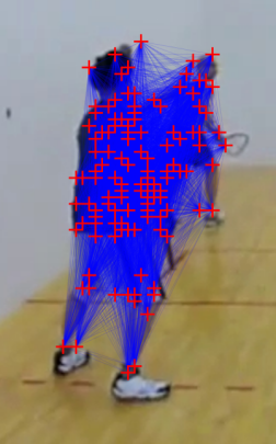
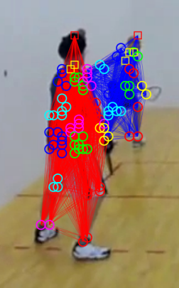
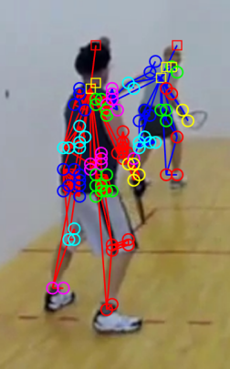
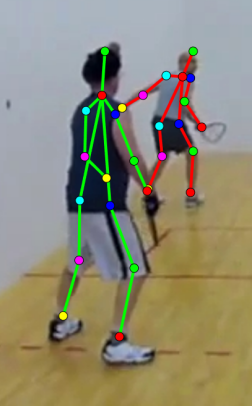
(a) raw input	(b) Deeper Cut [12]	(c) our approach	(d) final output

Figure 1: Overview of our approach. (a) Raw input which consists of unary terms (red crosses) and pairwise terms (blue connections). (b) [12] employs a fully-connected body model. (c) Our approach models the human body as an “augmented tree” graph. (d) We achieve more accurate results while being 100x faster than [12].

We also note that a more recent approach of [15] achieves considerable speed up over [12]: it is about three orders of magnitude faster than [12] while being 10x faster than our proposed method. Nevertheless, as will be shown later in experiments section, it is not as accurate as our method, especially for difficult-to-localize parts such as ankles and wrist.

Our paper is organized as follows. In Section 2 we outline the assumptions of our model and its structure, then formulate it more precisely as an ILP. In Section 3 we introduce our column generation approach for computing the optimal MPPE assignment, where the column generation steps are solved using efficient dynamic programming and small scale, exactly solvable integer programs (IP). In Section 4 we demonstrate that our model and inference process provide state of the art results for MPPE on benchmark data. Finally, we conclude and discuss extensions in Section 5. Additional derivations and discussion are provided in the supplements.

2 Multi-Person Pose Estimation Model

In this section, we describe our two-tiered structure for reasoning about pose estimation. The input to our model is a set of body part detections; in practice, we use the body part detector of [12], which employs a deep convolutional neural network [5, 14]. Each detection is associated with exactly one body part. Our model uses fourteen parts, consisting of the head and neck, along with right and left variants of the ankle, knee, hip, wrist, elbow, and shoulder. We use the term complete pose to describe a person in an image, as represented by the detections associated with their body parts.

2.1 Assignment of Parts and Validity

We partition the body parts into two types: major parts, of which at least one is required to be present (not occluded) in any complete pose, and minor parts, any of which may be occluded. In practice, we take the neck to be the only major part, thus requiring that each complete pose be associated with at least one neck detection.

We reason about the assignment of parts to a complete pose in two tiers: a local assignment, which corresponds to a grouping of detections for a single part that are all associated with a single complete pose; and a global pose, which corresponds to at most one detection of each part. In practice, the score of a local assignment evaluates the coherence of the detections for that part (for example, two visually similar detections of a part in close proximity are more likely to correspond to the same person), while the score of the global pose captures the coherence of these part locations according to a (nearly) tree structured model of the human body (for example, the head is typically located above the neck). In any local assignment, we require that exactly one detection be assigned to some global pose, so that the global pose reasons about the overall position and visibility of the person, and the local assignment captures any additional detections associated with each visible part. A complete pose corresponds to a single person in the image, and consists of a single global pose and the local assignments (additional detections) associated with each of its visible parts.

Finally, we categorize detections as either global, local, or false positive. Global detections are those associated with some global pose; local detections are the non-global detections in a local assignment; and false positives are detections not contained in any global pose or local assignment.

These definitions result in the following requirements for a set of complete poses, which describe a group of people in the image:

1. A detection can only be global, local, or neither.

2. No two global poses can share a common detection.

3. No two local assignments can share a common detection.

4. The global detection of a local assignment must also be included in a global pose.

We refer to these conditions as the validity conditions and a selection of global poses and local assignments that meet them is referred to as valid.

2.2 Integer Linear Program Formulation

Term	Form	Index	Meaning
$\mathcal{D}$	set	$d$	set of detections
$\mathcal{R}$	set	$r$	set of parts
$\mathcal{R}^{\prime}$	set	$r$	set of major parts; $\mathcal{R}^{\prime}\subseteq\mathcal{R}$
$R$	$\{0,1\}^{|\mathcal{D}|\times|\mathcal{R}|}$	$R_{dr}$,$R_{d}$	$R_{dr}=1$ indicates that detection $d$ is associated with part $r$.
$R_{d}$	$R_{d}\in\mathcal{R}$	none	short hand for $\mbox{arg}\max_{r}R_{dr}$
$\mathcal{G}$	set	$q$	set of all global poses
$\mathcal{L}$	set	$l$	set of all local assignments
$\hat{\mathcal{G}}$	set	$q$	set of global poses generated during column generation
$\hat{\mathcal{L}}$	set	$l$	set of local assignments generated during column generation
$\theta$	$\mathbb{R}^{|\mathcal{D}|}$	$d$	$\theta_{d}$ is the cost of including $d$ in a complete pose
$\phi$	$\mathbb{R}^{|\mathcal{D}|\times|\mathcal{D}|}$	$d_{1},d_{2}$	$\phi_{d_{1}d_{2}}$ is the cost of including $d_{1},d_{2}$ in the same local assignment or global pose
$G$	$\{0,1\}^{|\mathcal{D}|\times|\mathcal{G}|}$	$d,q$	$G_{dq}=1$ indicates that $d$ is a global detection in global pose $q$
$L$	$\{0,1\}^{|\mathcal{D}|\times|\mathcal{L}|}$	$d,l$	$L_{dl}=1$ indicates that $d$ is a local detection in local assignment $l$
$M$	$\{0,1\}^{|\mathcal{D}|\times|\mathcal{L}|}$	$d,l$	$M_{dl}=1$ indicates that $d$ is a global detection in local assignment $l$
$\Gamma$	$\mathbb{R}^{|\mathcal{G}|}$	$q$	$\Gamma_{q}$ is the cost of global pose $q$
$\Psi$	$\mathbb{R}^{|\mathcal{L}|}$	$l$	$\Psi_{l}$ is the cost of local assignment $l$
$\gamma$	$\{0,1\}^{|\mathcal{G}|}$	$q$	$\gamma_{q}=1$ indicates that global pose $q$ is selected.
$\psi$	$\{0,1\}^{|\mathcal{L}|}$	$l$	$\psi_{l}=1$ indicates that local assignment $l$ is selected.

Table 1: Summary of Notation

We now formally define the MPPE task as an integer linear program (ILP). We first describe the variables associated with detections and parts, global poses, and local assignments; give the validity constraints on these variables as linear inequalities; and finally define the cost of a pose and the overall optimization problem, and discuss its linear program (LP) relaxation. We summarize our notation in Table 1.

Detections and Parts.

We denote the set of detections in the image as $\mathcal{D}$, and index these detections by $d$. Similarly, we use $\mathcal{R}$ to denote the set of parts, indexed by $r$, and denote the set of major parts by $\mathcal{R}^{\prime}\subseteq\mathcal{R}$. We describe the mapping of detections to parts using a matrix $R\in\{0,1\}^{|\mathcal{D}|\times|\mathcal{R}|}$, indexed by $d,r$. Specifically, $R_{dr}=1$ indicates that detection $d$ is associated with part $r$. As a useful shorthand, we define $R_{d}$ to be the part associated with detection $d$.

Global Poses.

Given the set of detections $\mathcal{D}$, we define the set of all possible global poses over $\mathcal{D}$ as $\mathcal{G}$. Members of $\mathcal{G}$ have at least one global detection corresponding to a major part and no more than one detection corresponding to any given part. We describe mappings of detections to global poses using a matrix $G\in\{0,1\}^{|\mathcal{D}|\times|\mathcal{G}|}$, and set $G_{dq}=1$ if and only if detection $d$ is associated with global pose $q$.

Note that the set of all possible poses $\mathcal{G}$ is impractically large (it contains all valid assignments of detections to a global pose). Thus in practice, we never construct $G$ explicitly; instead, we maintain an active set of poses, $\hat{\mathcal{G}}$, restricting $G$ to this set.

Local Assignments.

Next we denote the set of all possible local assignments over the detections $\mathcal{D}$ by $\mathcal{L}$, and index these possible local assignments by $l$. Since we require that, for any local assignment $l\in\mathcal{L}$, exactly one of the detections in $l$ is global, we describe $\mathcal{L}$ using two matrices $L,M\in\{0,1\}^{|\mathcal{D}|\times|\mathcal{L}|}$, where $L_{dl}=1$ if and only if detection $d$ is associated with $l$ as a local (non-global) detection, and $M_{dl}=1$ if and only if detection $d$ is associated with $l$ as a global detection.

The set $\mathcal{L}$ is too large to be considered explicitly during optimization. We maintain a subset $\hat{\mathcal{L}}\subseteq\mathcal{L}$ during optimization, and explictly represent $L$ and $M$ restricted to $\hat{\mathcal{L}}$.

Validity Constraints.

We index a set of global poses and local assignments using indicator vectors, so that $\gamma\in\{0,1\}^{|\mathcal{G}|}$ with $\gamma_{q}=1$ to indicate that global pose $q\in\mathcal{G}$ is selected, and $\gamma_{q}=0$ otherwise. Similarly, we let $\psi\in\{0,1\}^{|\mathcal{L}|}$ with $\psi_{l}=1$ to indicate that local assignment $l\in\mathcal{L}$ is selected, with $\psi_{l}=0$ otherwise.

A solution $\gamma,\psi$ is a valid solution if and only if it satisfies the rules defined previously, which is written formally as the following set of linear inequalities:

$$G\gamma+L\psi \leq 1 :\ \mbox{A detection can only be global, local, or neither;}$$

no two global poses can share the same detection.

$$L\psi+M\psi \leq 1 :\ \mbox{No two local assignments can share the same detection.}$$

$$-G\gamma+M\psi \leq 0 :\ \mbox{The global detection of a local assignment is included in some global pose.}$$

Cost Function.

We now describe the cost function for MPPE. Our total cost is expressed in terms of unary costs $\theta\in\mathbb{R}^{|\mathcal{D}|}$, where $\theta_{d}$ is the cost of assigning detection $d$ to a pose, and pairwise costs $\phi\in\mathbb{R}^{|\mathcal{D}|\times|\mathcal{D}|}$, where $\phi_{d_{1}d_{2}}$ is the cost of assigning detections $d_{1}$ and $d_{2}$ to a common global pose or local assignment. We use $\omega$ to denote the cost of instancing a pose, which serves to regularize the number of people in an image.

The cost of a complete pose is thus the sum of the costs of the following.

• $\phi$ terms associated with pairs of detections in its global pose

• $\phi$ terms associated with pairs of detections within each of its local assignments

• $\theta$ terms associated with detections in either its global or local assignments

• $\omega$ term associated with instancing a pose.

For convenience, we separate these costs into $\Gamma_{q}$ as the cost associated with the global pose $q$, and $\Psi_{l}$ as the cost of local assignment $l$, respectively:

$$\Gamma_{q} =\omega+\sum_{d\in\mathcal{D}}\theta_{d}G_{dq}+\sum_{\begin{subarray}{c}d_{1}\in\mathcal{D}\\ d_{2}\in\mathcal{D}\end{subarray}}\phi_{d_{1}d_{2}}G_{d_{1}q}G_{d_{2}q}$$

$$\Psi_{l} =\sum_{d\in\mathcal{D}}\theta_{d}L_{dl}+\sum_{\begin{subarray}{c}d_{1}\in\mathcal{D}\\ d_{2}\in\mathcal{D}\end{subarray}}\phi_{d_{1}d_{2}}(L_{d_{1}l}+M_{d_{1}l})(M_{d_{2}l}+L_{d_{2}l})$$

Integer Linear Program.

We now cast the problem of finding the lowest cost set of poses as an integer linear program subject to our validity constraints:

$$\min_{\begin{subarray}{c}\gamma\in\{0,1\}^{|\mathcal{G}|}\\ \psi\in\{0,1\}^{|\mathcal{L}|}\end{subarray}} \Gamma^{\top}\gamma+\Psi^{\top}\psi G\gamma+L\psi\leq 1\quad L\psi+M\psi\leq 1 -G\gamma+M\psi\leq 0$$ s.t. (1)

By relaxing the integrality constraints on $\gamma,\psi$, we obtain a linear program relaxation of the ILP, and can convert Eq. (1) to its dual form using Lagrange multiplier sets $\lambda^{1},\lambda^{2},\lambda^{3}\in\mathbb{R}_{0+}^{|\mathcal{D}|}$:

$$\min_{\begin{subarray}{c}\gamma\geq 0\\ \psi\geq 0\\ G\gamma+L\psi\leq 1\\ L\psi+M\psi\leq 1\\ -G\gamma+M\psi\leq 0\end{subarray}}\Gamma^{\top}\gamma+\Psi^{\top}\psi=\max_{\begin{subarray}{c}\lambda^{1}\geq 0\\ \lambda^{2}\geq 0\\ \lambda^{3}\geq 0\\ \Gamma+G^{\top}(\lambda^{1}-\lambda^{3})\geq 0\\ \Psi+L^{\top}\lambda^{1}+(M^{\top}+L^{\top})\lambda^{2}+M^{\top}\lambda^{3}\geq 0\end{subarray}}-1^{\top}\lambda^{1}-1^{\top}\lambda^{2}$$ (2)

3 Column Generation Solution

In this section we consider optimization of the LP relaxation in Eq. (2). As discussed, the primary difficulty is the intractable sizes of the sets $\mathcal{G},\mathcal{L}$. Instead, we consider subsets $\hat{\mathcal{G}}\subseteq\mathcal{G}$ and $\hat{\mathcal{L}}\subseteq\mathcal{L}$ that are constructed strategically during optimization so as to be small, while still solving the LP in Eq. (2) exactly. This type of column generation approach is common in the operations research literature, in which the task of generating the columns is often called pricing [3].

We solve the dual form LP in Eq. (2) iteratively with two steps. We first solve the dual LP over constraint sets $\hat{\mathcal{G}}$ and $\hat{\mathcal{L}}$, which are initialized to be empty. Then, we identify violated constraints in the dual using combinatorial optimization and add these to sets $\hat{\mathcal{G}}$ and $\hat{\mathcal{L}}$. One local assignment is identified corresponding to each possible selection of a global detection, and one global pose is identified for each selection of a detection corresponding to a major part. We repeat these two steps until no more violated constraints exist. We then solve the integer linear program over sets $\hat{\mathcal{G}}$ and $\hat{\mathcal{L}}$. We diagram this procedure in Figure 3 and show the corresponding algorithm in Alg  1.

Algorithm 1 Dual Optimization

1:  $\hat{\mathcal{G}}\leftarrow\{\}$

2:  $\hat{\mathcal{L}}\leftarrow\{\}$

3:  repeat

4:     $\lambda\leftarrow$ Maximize dual in Eq. (2) over column sets $\hat{\mathcal{G}},\hat{\mathcal{L}}$

5:     for $d_{*}\in\mathcal{D}$ do

6:        $l_{*}\leftarrow\mbox{arg}\min_{\begin{subarray}{c}l\in\mathcal{L}\\ M_{d_{*}l}=1\end{subarray}}(\lambda^{3}_{d_{*}}+\lambda^{2}_{d_{*}})M_{d_{*}l}+\sum_{d\in\mathcal{D}}(\lambda^{1}_{d}+\lambda^{2}_{d})L_{dl}+\Psi_{l}$

7:        if $(\lambda^{3}_{d_{*}}+\lambda^{2}_{d_{*}})M_{d_{*}l_{*}}+\sum_{d\in\mathcal{D}}(\lambda^{1}_{d}+\lambda^{2}_{d})L_{dl_{*}}+\Psi_{l_{*}}<0$ then

8:           $\dot{\mathcal{L}}\leftarrow[\dot{\mathcal{L}}\cup l_{*}]$

9:        end if

10:     end for

11:     for $d_{*}\in\mathcal{D}$ s.t. $R_{d_{*}}$ $\in\mathcal{R}^{\prime}$ do

12:        $q_{*}\leftarrow\mbox{arg}\min_{\begin{subarray}{c}q\in\mathcal{G}\\ G_{d_{*}q}=1\end{subarray}}\Gamma_{q}+\sum_{d\in\mathcal{D}}G_{dq}(\lambda^{1}_{d}-\lambda^{3}_{d})$

13:        if $\Gamma_{q_{*}}+\sum_{d\in\mathcal{D}}G_{dq_{*}}(\lambda^{1}_{d}-\lambda^{3}_{d})<0$ then

14:           $\dot{\mathcal{G}}\leftarrow[\dot{\mathcal{G}}\cup q_{*}]$

15:        end if

16:     end for

17:     $\hat{\mathcal{L}}\leftarrow[\hat{\mathcal{L}},\dot{\mathcal{L}}]$

18:     $\hat{\mathcal{G}}\leftarrow[\hat{\mathcal{G}},\dot{\mathcal{G}}]$

19:  until  $|\dot{\mathcal{G}}|+|\dot{\mathcal{L}}|=0$

3.1 Identifying Violated Local Assignments

For each detection $d_{*}\in\mathcal{D}$, we compute the most violated constraint corresponding to a local assignment in which $d_{*}$ is the global detection. We write this as an IP using the indicator vector $x\in\{0,1\}^{|\mathcal{D}|}$, and define a new column $l$ for inclusion in matrices $L$ and $M$, assigning $M_{d^{*}l}=1$ and $L_{dl}=x^{*}_{d}$ for all $d\in\mathcal{D}$, where $x^{*}$ is the solution to

$$\min_{\begin{subarray}{c}l\in\mathcal{L}\\ M_{d_{*}l}=1\end{subarray}}(\lambda^{2}_{d_{*}}+\lambda^{3}_{d_{*}})M_{d_{*}l}+\sum_{d\in\mathcal{D}}(\lambda^{1}_{d}+\lambda^{2}_{d})L_{dl}+\Psi_{l}$$

$$= \min_{\begin{subarray}{c}x\in\{0,1\}^{|\mathcal{D}|}\\ x_{d_{*}}=1\\ x_{d}=0\;\;\forall R_{d}\neq R_{d_{*}}\end{subarray}}(\lambda^{2}_{d_{*}}+\lambda^{3}_{d_{*}})+\sum_{d\in\mathcal{D}\setminus d_{*}}(\theta_{d}+\lambda^{1}_{d}+\lambda^{2}_{d})x_{d}+\sum_{d_{1},d_{2}\in\mathcal{D}}x_{d_{1}}x_{d_{2}}\phi_{d_{1}d_{2}}$$ (3)

In practice, we solve this IP by explicit enumeration over the possible local assignments. Since the number of detections associated with any given part (and thus eligible to participate in the local assignment of $d^{*}$) is small – no larger than 15 and usually less than 10 – exhaustive search is feasible. One can convert this problem to an equivalent ILP problem and use an off-the-shelf ILP solver that employs branch-and-cut to solve it.

3.2 Identifying Violated Global Poses

For each detection $d_{*}$ such that $R_{d_{*}}\in\mathcal{R}^{\prime}$ (i.e., $d_{*}$ corresponds to a major part), we compute the most violated constraint corresponding to a global pose that includes detection $d_{*}$. Again, we write this as an IP using an indicator vector $x\in\{0,1\}^{|\mathcal{D}|}$, and define a new column $q$ to be included in $G$, defined by $G_{dq}=x^{*}_{d}$ for all $d\in\mathcal{D}$, where $x^{*}$ is the solution to:

$$\min_{\begin{subarray}{c}q\in\mathcal{G}\\ G_{d_{*}q}=1\end{subarray}}\Gamma_{q}+\sum_{d\in\mathcal{D}}G_{dq}(\lambda^{1}_{d}-\lambda^{3}_{d})\quad=\quad\omega+\!\!\!\!\!\!\min_{\begin{subarray}{c}x\in\{0,1\}^{|\mathcal{D}|}\\ x_{d_{*}}=1\\ \sum_{d\in\mathcal{D}}R_{dr}x_{d}\leq 1\;\;\forall r\in\mathcal{R}\end{subarray}}\!\!\!\!\!\!\!\sum_{d\in\mathcal{D}}(\theta_{d}+\lambda^{1}_{d}-\lambda^{3}_{d})x_{d}+\sum_{d_{1}d_{2}\in\mathcal{D}}\phi_{d_{1}d_{2}}x_{d_{1}}x_{d_{2}}$$ (4)

By enforcing some structure in the pairwise costs $\phi$, we can ensure that this optimization problem is tractable. A common model in computer vision is to represent the location of parts in the body using a tree-structured model, for example in the deformable part model of [7, 6, 21]; this forces the $\phi$ terms to be zero between non-adjacent parts on the tree.

In our application we augment this tree model with additional edges from the major part (i.e., the neck) to all other non-adjacent body parts. This is illustrated in Fig 2. Then, given the global detection associated with the neck, the conditional model is tree-structured and can be optimized using dynamic programming in $O(|\mathcal{R}|k^{2})$ time, where $k$ is the maximum number of detections per part ($k<15$ in practice).

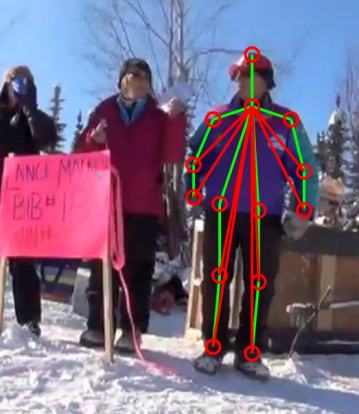
(a) augmented-tree for global pose

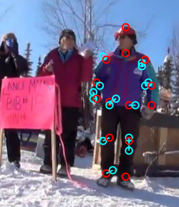
(b) fully-connected graph for local assignment

Figure 2: Graphical representation of our pose model. (a) A global pose is modeled by an augmented-tree, in which each red node represents a global detection, green edges are connections of traditional pictorial structure, while red edges are augmented connections from neck to all non-adjacent parts of neck. (b) Each local assignment is modeled by a fully-connected graph, where red node represents the global detection in this local assignment, while cyan nodes represents local detections.

Figure 3: Diagram of our system: blue blocks represent steps for generating unary and pairwise costs, which are identical to that of [12]. Cost generator is the procedure for mapping the output scores of the deep neural network to unary cost terms and computing pairwise costs based on geometric features. Green blocks represent steps for generating columns. Opt Local and Opt Global correspond to the pricing problems in line 5-10 and line 11-16 of Alg 1, respectively. The brown block represents a dual LP solver while red blocks show steps for producing the final integer solutions at termination.

4 Experiments

Part	Head	Shoulder	Elbow	Wrist	Hip	Knee	Ankle	mAP(UBody)	mAP	time (s/frame)
Ours	93.3	89.6	79.8	70.1	78.8	73.2	66.6	83.2	79.1	2.7
[15]	93.4	89.7	79.1	68.6	78.8	72.5	65.2	82.7	78.5	0.16
[12]	92.4	88.9	79.1	67.9	78.7	72.4	65.4	82.1	78.1	270*

Table 2: We display average precision of our approach versus the baselines for the various human parts as well as whole body. Running times are measured on an Intel i7-6700 quad-core CPU. Note that due to software and hardware limitations we cannot run [12] on our own machine and thus we directly cite the running time on validation set which was reported in their paper.

Deeper Cut [12]
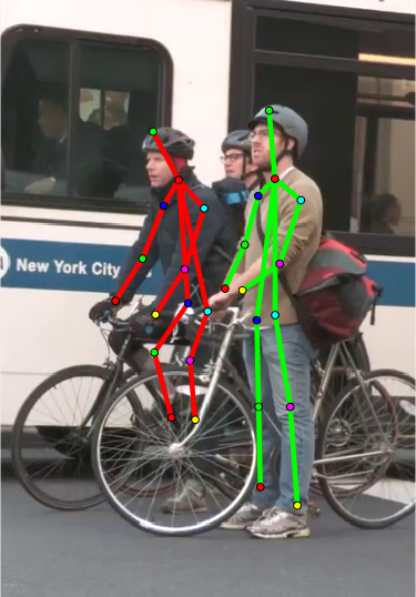
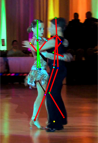
Our Approach

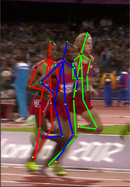
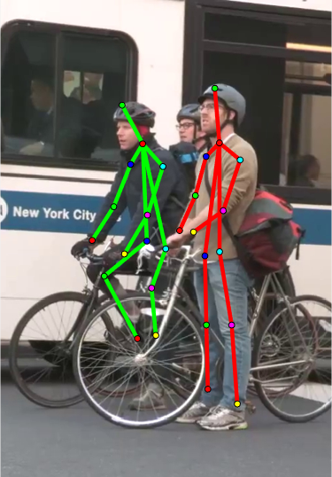
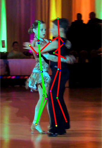
Figure 4: Qualitative comparison of [12] (top row) and our approach (bottom row). (Left column) [12] occasionally fails and produces many false positives per detection, while our approach avoid this by enforcing the fact that each individual person must have a neck. (Middle column) We predict left knee of the person on the left better than [12]. (Right column) [12] fails to find the lower body parts of the person on the left and confuses ankle and kneel of the two people, while we successfully avoid these errors.

4.1 Experiment Setup

We evaluate our approach in terms of the Average Precision (AP) on the of MPII–Multiperson training set [1], which consists of 3844 images. For a fair comparison, we use the unary and pairwise costs directly provided by Insafutdinov et al., and did not modify or weight these costs in any way for any approach considered in this experiment. Our model thus only differs from [12] and [15] in that our two-tier structure defines a distinct and novel cost function. In particular, our introduction of the two-tier structure forces us to ignore the pairwise $\phi$ terms corresponding to interactions between non-global detections that are associated with different parts in a given pose. A major benefit of this difference is a fast and typically exact optimization process. Besides, local detections in a local assignment often do not align well with the ground-truth position of a body-part (e.g. Figure 1 and 2), thus pairwise interactions between such detections across part types can be noisy due to inaccurate localization, and ignoring such interactions may contribute to more accurate localization of body-parts.

In addition to the structure depicted in Figure 2(a), we found that adding additional edges for global pose that does not break the conditional tree structure slightly improves Mean Average Precision (mAP) from 78.8 to 79.1 with negligible increase in running time. The additional edges we employ in our final model are left-hip to left-shoulder, right-hip to right-shoulder and shoulders to head.

We set $\omega=30$ heuristically to discourage the selection of global poses that include few detections, which tend to be lower magnitude in their cost. After solving the LP (2), we tighten the relaxation if necessary using odd set inequalities of size three [10, 20], which does not interfere with pricing; more details can be found in the supplements. In practice, however, we find that these refinements are rarely necessary to produce integer solutions with identical cost to the LP relaxation at termination.

We compare our results against two baselines: 1) [12], whose results are obtained by its authors upon our request due to our limited acess to computing resources and commercial LP solvers. 2) [15], whose results are obtained via running their code over the costs from [12]. We found that employing the augmented-tree structure instead of a fully-connected structure gives [15] sligntly better performance (from 78.4 to 78.5). Note that even based on the same graph structure, [15] still has more pairwise connections than our model as it considers connections between all detections from different parts.

4.2 Benchmark Results

As shown in Table 2, our approach runs much faster than [12] due to both the reduced model size and our more sophisticated inference algorithm. While [15] runs about 10x faster than our approach, we achieve more accurate results than it: the improvement in mAP might seem small (78.5 to 79.1), however we achieve much better AP on difficult-to-localize parts such as wrist (70.1 versus 68.6) and ankle (66.6 versus 65.2), while we only use a subset of edges compared to [12] and [15]. Also keep in mind that all experiments are based on the same set of unary/pairwise costs without any form of learning, thus our improvement is solely due to our novel modeling for MPEE problem and the ability to find global minimum of our cost.

We also note that the code of [15] is in pure C++ and is heavily optimized, while our code is in pure Python and we did not take advantage of the parallelizable nature of our pricing problems. Nevertheless, we still achieve considerable speed up over [12]. We will release the code and data we used upon acceptance of this paper.

5 Conclusion

We introduce a new formulation of the multi-person pose estimation problem, along with a novel inference algorithm based on column generation that admits efficient inference. We compare our results to a state of the art algorithm and demonstrate that our approach rapidly produces more accurate results than the baseline.

In future work we intend to apply our method to other domains where similar local/global structure is present, and can assist in non-maximum suppression or clustering, for example in relevant ILP optimization formulations of multi-object tracking [18], moral lineage tracking[13], and MPPE tasks on video [11].

Appendix A Tighter Bound for Multi-Person Pose Estimation

A tighter LP relaxation than that in the main paper can be motivated by the following observations: (1) no more than one global pose can include more than two members of a given set of three detections. (2) No more than one local assignment can include more than two members of a given set of three detections (either as local or global). These constraints are called odd set inequalities of order three [10]. We formalize this below.

We refer to the set of all sets of three unique detections (triples) as $\mathcal{C}$. We use $C^{\mathcal{L}}\in\{0,1\}^{|\mathcal{C}|\times|\mathcal{L}|}$ to define the adjacency matrix between triples and local assignments. Similarly we use $C^{\mathcal{G}}\in\{0,1\}^{|\mathcal{C}|\times|\mathcal{G}|}$ to define the adjacency matrix between triples and global poses. Here $C^{\mathcal{L}}_{cl}=1$ if and only if local assignment $l$ contains two or more members of set $c$. Similarly we set $C^{\mathcal{G}}_{cq}=1$ if and only if global pose $q$ contains two or more members of set $c$. We define $C^{\mathcal{L}},C^{\mathcal{G}}$ formally below.

$$C^{\mathcal{G}}_{cq}=[(\sum_{d\in c}G_{dq})\geq 2] \quad\forall c\in\mathcal{C},q\in\mathcal{G}$$ (5)

$$C^{\mathcal{L}}_{cl}=[(\sum_{d\in c}L_{dl}+M_{dl})\geq 2] \quad\forall c\in\mathcal{C},l\in\mathcal{L}$$

A.1 Dual Form

We now write the corresponding primal LP for multi-person pose estimation with triples added.

$$\min_{\begin{subarray}{c}\gamma\geq 0\\ \psi\geq 0\\ G\gamma+L\psi\leq 1\\ L\psi+M\psi\leq 1\\ -G\gamma+M\psi\leq 0\\ C^{\mathcal{G}}\gamma\leq 1\\ C^{\mathcal{L}}\psi\leq 1\end{subarray}}\Gamma^{\top}\gamma+\Psi^{\top}\psi$$ (6)

The constraints $C^{\mathcal{G}}\gamma\leq 1$ and $C^{\mathcal{L}}\psi\leq 1$ are referred to as “rows" of the primal problem. We now take the dual of Eq. (6). This induces two additional sets of Lagrange multipliers $\lambda^{4},\lambda^{5}\in\mathbb{R}_{0+}^{\mathcal{C}}$. We now write the dual below.

$$\max_{\begin{subarray}{c}\lambda\geq 0\\ \Gamma+G^{\top}(\lambda^{1}-\lambda^{3})+C^{\mathcal{G}\top}\lambda^{4}\geq 0\\ \Psi+L^{\top}\lambda^{1}+(M^{\top}+L^{\top})\lambda^{2}\\ +M^{\top}\lambda^{3}+C^{\mathcal{L}\top}\lambda^{5}\geq 0\end{subarray}}-1^{\top}\lambda^{1}-1^{\top}\lambda^{2}-1^{\top}\lambda^{4}-1^{\top}\lambda^{5}$$ (7)

A.2 Algorithm

In order to tackle optimization we introduce subsets of $\mathcal{C}^{\mathcal{G}}$ and $\mathcal{C}^{\mathcal{L}}$, denoted $\hat{\mathcal{C}}^{\mathcal{G}}$ and $\hat{\mathcal{C}}^{\mathcal{L}}$ respectively. These subsets are intially empty and grow only when needed. We write an optimization algorithm below in Alg 2 with subroutines $\mbox{ROW}(\gamma,\psi)$ (Section A.3) and $\mbox{COLUMN}(\lambda)$ (Section A.4) describing the generation of new triples and columns respectively.

Algorithm 2 Column/Row Generation

  $\hat{\mathcal{G}}\leftarrow\{\}$

  $\hat{\mathcal{L}}\leftarrow\{\}$

  $\hat{\mathcal{C}}^{\mathcal{G}}\leftarrow\{\}$

  $\hat{\mathcal{C}}^{\mathcal{L}}\leftarrow\{\}$

  repeat

     $[\lambda]\leftarrow$ Maximize dual in Eq (7) over column and rows sets $\hat{\mathcal{G}},\hat{\mathcal{L}},\hat{\mathcal{C}}^{\mathcal{L}},\hat{\mathcal{G}}^{\mathcal{L}}$

     Recover $\gamma$ from $\lambda$

     $\dot{\mathcal{G}},\dot{\mathcal{L}}\leftarrow\mbox{COLUMN}(\lambda)$

     $\dot{\mathcal{C}}^{\mathcal{L}},\dot{\mathcal{C}}^{\mathcal{G}}\leftarrow\mbox{ROW}(\gamma,\psi)$

     $\hat{\mathcal{G}}\leftarrow[\hat{\mathcal{G}},\dot{\mathcal{G}}]$

     $\hat{\mathcal{L}}\leftarrow[\hat{\mathcal{L}},\dot{\mathcal{L}}]$

     $\hat{\mathcal{C}}^{\mathcal{L}}\leftarrow[\hat{\mathcal{C}}^{\mathcal{L}},\dot{\mathcal{C}}^{\mathcal{L}}]$

     $\hat{\mathcal{C}}^{\mathcal{G}}\leftarrow[\hat{\mathcal{C}}^{\mathcal{G}},\dot{\mathcal{C}}^{\mathcal{G}}]$

  until  $\dot{\mathcal{G}}=[]$ and $\dot{\mathcal{L}}=[]$ and $\dot{\mathcal{C}}=[]$

A.3 Generating rows

Generating rows corresponding to local assignments is done separately for each part. We write the corresponding optimization for identifying the most violated constraint corresponding to a local assignment over a given part $r$ as follows.

$$\max_{\begin{subarray}{c}c\in\mathcal{C}\\ R_{d}=r\;\;\forall d\in c\end{subarray}}\sum_{q\in\mathcal{L}}C^{\mathcal{L}}_{cl}\psi_{q}$$ (8)

Finding violated rows corresponding to global poses is assisted by the knowledge that one need only consider triples over three unique part types as no global pose includes two or more detections of a given part. Hence only such triples need be considered for global pose. For any given $c$ let the detections associated with it be $c=\{d_{c_{1}}d_{c_{2}}d_{c_{3}}\}$, the corresponding optimization can then be written as below:

$$\max_{\begin{subarray}{c}c\in\mathcal{C}\\ R_{d_{c_{1}}}\neq R_{d_{c_{2}}}\\ R_{d_{c_{1}}}\neq R_{d_{c_{3}}}\\ R_{d_{c_{2}}}\neq R_{d_{c_{3}}}\end{subarray}}\sum_{q\in\mathcal{G}}C^{\mathcal{G}}_{cq}\gamma_{q}$$ (9)

Triples are only added to $\hat{\mathcal{C}}^{\mathcal{L}},\hat{\mathcal{C}}^{\mathcal{G}}$ if the corresponding constraint is violated.

A.4 Generating Columns

Generating columns is considered separately for global poses and local assignments. The corresponding equations are unmodified from the main document except for the introduction of terms over triples. We write the IP for generating the most violated constraint corresponding to a local assignment given the global detection below.

$$\min_{\begin{subarray}{c}x\in\{0,1\}^{|\mathcal{D}|}\\ x_{d_{*}}=1\end{subarray}}(-\lambda^{1}_{d_{*}}+\lambda^{3}_{d_{*}}-\theta_{d_{*}})+\sum_{d\in\mathcal{D}}(\theta_{d}+\lambda^{1}_{d}+\lambda^{2}_{d})x_{d}$$ (10)

$$+\sum_{d_{1},d_{2}\in\mathcal{D}}\phi_{d_{1}d_{2}}x_{d_{1}}x_{d_{2}}+\sum_{c\in\mathcal{C}^{\mathcal{L}}}\lambda^{5}_{cl}[\sum_{d\in c}x_{d}\geq 2]$$

We optimize Eq. (10) via explicit enumeration as described in the main paper.

For each $d_{*}$ such that $R_{d_{*}}\in\mathcal{R}^{\prime}$ we compute the most violated constraint corresponding to a global pose including $d_{*}$. We write this as an IP below.

$$\min_{\begin{subarray}{c}x\in\{0,1\}^{|\mathcal{D}|}\\ x_{d_{*}}=1\\ \sum_{d\in\mathcal{D}}R_{dr}x_{d}\leq 1\;\;\forall r\in\mathcal{R}\end{subarray}}\sum_{d\in\mathcal{D}}(\theta_{d}+\lambda^{1}_{d}-\lambda^{3}_{d})x_{d}$$ (11)

$$+\sum_{d_{1}d_{2}\in\mathcal{D}}\phi_{d_{1}d_{2}}x_{d_{1}}x_{d_{2}}+\sum_{c\in\mathcal{C}^{\mathcal{G}}}\lambda^{4}_{cq}[\sum_{d\in c}x_{d}\geq 2]$$

The introduction of triples breaks the structure of the problem, thus we can no longer optimize Eq. (11) via dynamic programming. We found that employing the branch and bound algorithm proposed by [20] is not computationally problematic for our problems as the number of triplets needed for convergence is small.

Appendix B Additional Statistics for Results on MPII Training Set

With up to 150 detections per image, we found our column generation solver usually terminates with a few hundreds, and no more than 1000 columns (i.e. total number of global poses and local assignments).

Out of all 3844 instances, we observe fractional LP solutions on 131 instances, 45 of which we successfully reached integer solutions with the help of triplets constraints; for the rest of 86 fractional instances, it costs negligible additional time to run trial version of CPLEX ILP solver to obtain integer solutions given columns we generated.

References

- [1] M. Andriluka, L. Pishchulin, P. Gehler, and B. Schiele. 2d human pose estimation: New benchmark and state of the art analysis. In Proc. of CVPR, 2014.
- [2] P. Baldi, P. Sadowski, and D. Whiteson. Searching for exotic particles in high-energy physics with deep learning. Nature communications, 5(4308), 2014.
- [3] C. Barnhart, E. L. Johnson, G. L. Nemhauser, M. W. P. Savelsbergh, and P. H. Vance. Branch-and-price: Column generation for solving huge integer programs. Operations Research, 46:316–329, 1996.
- [4] N. Dalal and B. Triggs. Histograms of oriented gradients for human detection. In Proc. of CVPR, 2005.
- [5] C. Farabet, C. Couprie, L. Najman, and Y. LeCun. Learning hierarchical features for scene labeling. IEEE Transactions on Pattern Analysis and Machine Intelligence, 35(8):1915–1929, 2013.
- [6] P. Felzenszwalb, D. McAllester, and D. Ramanan. A discriminatively trained, multiscale, deformable part model. In Proc. of CVPR, 2008.
- [7] P. F. Felzenszwalb, R. B. Girshick, D. McAllester, and D. Ramanan. Object detection with discriminatively trained part-based models. IEEE transactions on pattern analysis and machine intelligence, 32(9):1627–1645, 2010.
- [8] P. F. Felzenszwalb and D. P. Huttenlocher. Pictorial structures for object recognition. International journal of computer vision, 61(1):55–79, 2005.
- [9] P. Gilmore and R. Gomory. A linear programming approach to the cutting-stock problem. Operations Research (volume 9), 1961.
- [10] O. Heismann and R. Borndörfer. A generalization of odd set inequalities for the set packing problem. In Operations Research Proc., 2014.
- [11] E. Insafutdinov, M. Andriluka, L. Pishchulin, S. Tang, E. Levinkov, B. Andres, and B. Schiele. ArtTrack: Articulated multi-person tracking in the wild. In Proc. of CVPR, 2017.
- [12] E. Insafutdinov, L. Pishchulin, B. Andres, M. Andriluka, and B. Schiele. Deepercut: A deeper, stronger, and faster multi-person pose estimation model. CoRR, abs/1605.03170, 2016.
- [13] F. Jug, E. Levinkov, C. Blasse, E. W. Myers, and B. Andres. Moral lineage tracing. In Proc. of CVPR, 2016.
- [14] A. Krizhevsky, I. Sutskever, and G. E. Hinton. Imagenet classification with deep convolutional neural networks. In Proc. of NIPS, 2012.
- [15] E. Levinkov, J. Uhrig, S. Tang, M. Omran, E. Insafutdinov, A. Kirillov, C. Rother, T. Brox, B. Schiele, and B. Andres. Joint graph decomposition and node labeling: Problem, algorithms, applications. In Proc. of CVPR, 2017.
- [16] L. Pishchulin, E. Insafutdinov, S. Tang, B. Andres, M. Andriluka, P. Gehler, and B. Schiele. DeepCut: Joint subset partition and labeling for multi person pose estimation. In Proc. of CVPR, 2016.
- [17] D. E. Rumelhart, G. E. Hinton, and R. J. Williams. Parallel Distributed Processing: Explorations in the Microstructure of Cognition, Vol. 1. MIT Press, Cambridge, MA, USA, 1986.
- [18] S. Tang, B. Andres, M. Andriluka, and B. Schiele. Subgraph decomposition for multi-target tracking. In Proc. of CVPR, 2015.
- [19] C. Vondrick, A. Khosla, T. Malisiewicz, and A. Torralba. Hoggles: Visualizing object detection features. In Proc. of ICCV, 2013.
- [20] S. Wang, S. Wolf, C. Fowlkes, and J. Yarkony. Tracking objects with higher order interactions using delayed column generation. In Proc. of AISTATS, 2017.
- [21] Y. Yang and D. Ramanan. Articulated pose estimation with flexible mixtures-of-parts. In Proc. of CVPR, 2011.