SANC: the process $\gamma\gamma\rightarrow ZZ$
SANC: процесс $\gamma\gamma\rightarrow ZZ$

Abstract

Рассматривается внедрение процесса $\gamma\gamma\to ZZ$ в систему SANC на однопетлевом уровне точности в мультиканальном подходе. Полученные однопетлевые скалярные форм факторы могут быть использованы в любом канале после соответствующей перестановки их аргументов – Мандельштамоских переменных $s,t,u$. Для проверки корректности результатов наблюдается независимость скалярных форм факторов от калибровочных параметров и выполнение тождества Варда (поперечность по внешнему фотону). Представлен полностью аналитический результат для тензорной структуры, ковариантной и спиральных амплитуд для данного процесса. Проведено расширенное сравнение аналитических и численных результатов с имеющимися данными в литературе.

The implementation of the process $\gamma\gamma\to ZZ$ at the one-loop level within SANC system multi-channel approach is considered. The derived one-loop scalar form factors can be used for any cross channel after an appropriate permutation of their arguments – Mandelstam variables $s,t,u$. To check of the correctness of the results we observe the independence of the scalar form factors on the gauge parameters and the validity of Ward identity (external photon transversality). We present the complete analytical results for the covariant and tensor structures and helicity amplitudes for this process. We make an extensive comparison of our analytical and numerical results with those existing in the literature.

^a Dzhelepov Laboratory for Nuclear Problems, JINR,
ul. JoliotC̣urie 6, RU1̣41980 Dubna, Russia; ^b Bogoliubov Laboratory of Theoretical Physics, JINR,
ul. JoliotC̣urie 6, RU1̣41980 Dubna, Russia;
^c Petersburg Nuclear Physics Institute, Gatchina, 188300, Russia.

PACS: 12.15.$-$y; 12.20.$-$m

1 Introduction

Physics with $\gamma\gamma$ collider [1], [2],[3] [4] and with $e^{+}e^{-}$ linear collider [5], [6], [7] always demonstrated the great interest to establish the effects from transversal and longitudinal polarization. We begin to create the theoretical support for the $\gamma\gamma$ colliders: first of all it is SANC modules for processes $\gamma\gamma\to\gamma\gamma(\gamma Z,ZZ$ at the one loop level [8],[9]. Second step will be MC generator with these modules taking into account the polarization effects for $\gamma\gamma$ and $e^{+}e^{-}$ physics.

In this article we describe some results obtained with SANC (Support of Analytic and Numerical calculations for experiments at Colliders) — a network system for semi-automatic calculations for processes of elementary particle interactions at the one-loop precision level, see  [10]. The corresponding FORTRAN modules  [11] for processes at the one loop level can be downloaded by request.

All calculations at the one-loop precision level are realized in the spirit of the book  [12] in the $R_{\xi}$ gauge and all the results are reduced up to the scalar Passarino–Veltman functions: $A_{0},\,B_{0},\,C_{0},\,D_{0}$  [13]. These two distinctive features allow one to perform several checks: e.g. to test gauge invariance by observing the cancellation of gauge parameter dependence, to test symmetry properties and validity of the Ward identities, all at the level of analytical expressions. The SANC system is based on FORM  [14] applications. These applications had to be modularized as procedures in a most universal way so as to be used as building blocks for the computation of more complex processes. We used a covariant method for calculating helicity amplitudes (HA) presented in [15]. The numerical computations are done in FORTRAN.

We have implemented in the framework of the SANC system processes such as

$$\gamma(p_{1},\lambda_{1})+\gamma(p_{2},\lambda_{2})\longrightarrow Z(p_{3},\lambda_{3})+Z(p_{4},\lambda_{4})$$ (1)

($\lambda_{i},\ (i=1,2,3,4)$ are the helicities of the external particles) in the Standard Model (SM) at the one-loop level of accuracy in $R_{\xi}$-gauge through fermion loops and corresponding precomputation blocks.

The computations of these processes take into account non-zero masses of loop-fermions. Our previous evaluation for processes $\gamma+\gamma\longrightarrow\gamma+\gamma$ and $\gamma+\gamma\longrightarrow\gamma+Z,Z\longrightarrow\gamma\gamma\gamma$ was presented in [8] and [9]. The additional precomputation modules used to calculate massive fermion-box diagrams are briefly described.

We discuss the covariant and tensor structures and present them in a compact form. The helicity amplitude approach and their expressions are given.

First of all we calculate $bbbb\to 0$ in the multi-channel approach and get the main object form factors (FF) for the annihilation to vacuum. In the second step we produce the FF of the real channel 1 by a permutation of the arguments $s,t$ and $u$.

The 4-momenta of incoming bosons are denoted by $p_{1}$ and $p_{2}$, of the outgoing ones by $p_{3}$ and $p_{4}$.

The 4-momenta conservation reads

$$p_{1}+p_{2}-p_{3}-p_{4}=0\,.$$

The Mandelstam variables are

$$s=~{}(p_{1}+p_{2})^{2},~{}t=-(p_{1}-p_{3})^{2},~{}u=-(p_{1}-p_{4})^{2}.$$

Whenever possible, we compare the results with those existing in the literature.

To check our numerical and analytical results we compare them with other independent calculations [16].

The paper is organized as follows. In section 2 we briefly describe the precomputation strategy (see also, [10]). In section 3 we discuss the tensor structures of covariant amplitudes for these processes and present their compact form. The idea of form factors is described in section 4. In section 5 we consider the sets of the corresponding helicity amplitudes. In the conclusions, section 6, we present the comparison of our results with those existing in the literature.

2 Precomputation strategy

In this section we briefly describe the modules relevant for $bb\to bb$, ($b$ - is $A$ or $Z$). The contributions of fermionic loop boxes form a gauge-invariant and UV-finite subset.

In SANC, the idea of precomputation becomes vitally important for boxes [10]. The calculation of some boxes for some particular processes takes so much time that an external user should refrain from repeating the precomputation. Furthermore, the richness of boxes requires a classification. Depending on the type of external lines ($f$ – fermion or $b$ – boson), we distinguish three large classes of boxes: $ffff$, $ffbb$ and $bbbb$.

The precomputation file bbbb Box, i.e. AAAA Box, AAAZ Box, AAZZ Box contains the sequence of procedures to calculate the covariant amplitude. At this step we suppose that all momenta are incoming (denoted by $p_{i}$) and photons are not on-mass-shell. Therefore, these results can be used for other processes which need these parts as building blocks.

When we implement the processes $bb\to bb$, we use this building block several times by replacing the incoming momenta $p_{i}$ by the corresponding kinematical momenta $k_{i}$, calculate FFs by the module bb->bb (FF), then helicity amplitudes by the modules bb->bb (HA) and finally the differential and total process cross section by the module bb->bb (XS).

3 Covariant amplitude

The covariant one-loop amplitude (CA) corresponds to the result of the straightforward standard calculation of all diagrams contributing to a given process at the one-loop (1-loop) level. The CA is being represented in a certain basis, made of strings of Dirac matrices and/or external momenta (structures), contracted with polarization vectors of vector bosons, $\epsilon(k)$, if any.

A CA can be written in an explicit form with the aid of scalar FFs.

$${\cal A}_{\gamma\gamma\to ZZ}=4e^{4}Q^{4}_{f}\sum\limits_{i=1}^{20}\left[{\cal F}^{\tt bos}_{i}\left(s\,,t\,,u\right)+{\cal F}^{\tt fer}_{i}\left(s\,,t\,,u\right)\right]T_{i}^{\alpha\beta\mu\nu}\,.$$

All masses, kinematical factors and coupling constant and other parameter dependences are included into these FFs ${\cal F}_{i}$, but tensor structure with Lorenz indexes made of strings of Dirac matrices are given by basis. The number of form factors is equal to the number of independent structures.

The covariant amplitude for the channel $bb\rightarrow bb$, i.e. $\gamma\gamma\rightarrow ZZ$ can be obtained from annihilation to the vacuum with the following permutations of the 4-momenta:

$$p_{1}\to p_{1},~{}p_{2}\to p_{2},~{}p_{3}\to-p_{3},~{}p_{4}\to-p_{4}.$$

To describe the tensor structures of the CA for $AA\to ZZ$ we introduce the following five auxiliary tensorial strings:

$$\tau_{1}^{ij} = p^{1i}p^{2j}+\frac{1}{2}s\delta^{ij},\quad\tau_{2}^{ij}=p^{2i}p^{3j}-\frac{1}{2}(M_{\scriptscriptstyle{Z}}^{2}-t)\delta^{ij},$$

$$\tau_{3}^{ij} = p^{1i}p^{3j}-\frac{1}{2}(M_{\scriptscriptstyle{Z}}^{2}-u)\delta^{ij},$$

$$\tau_{4}^{i} = p^{3i}+\frac{M_{\scriptscriptstyle{Z}}^{2}-t}{s}p^{1i},\quad\tau_{5}^{i}=p^{3i}+\frac{M_{\scriptscriptstyle{Z}}^{2}-u}{s}p^{2i}.$$

Our basis of CA is given by:

$$T_{1}^{\alpha\beta\mu\nu} = \tau_{1}^{\beta\alpha}p^{1\mu}p^{1\nu},\quad T_{2}^{\alpha\beta\mu\nu}=\tau_{1}^{\beta\nu}\tau_{1}^{\mu\alpha},\quad T_{3}^{\alpha\beta\mu\nu}=\tau_{1}^{\beta\nu}\tau_{3}^{\mu\alpha},\quad T_{4}^{\alpha\beta\mu\nu}=\tau_{1}^{\beta\mu}\tau_{1}^{\nu\alpha},$$

$$T_{5}^{\alpha\beta\mu\nu} = \tau_{1}^{\beta\mu}\tau_{3}^{\nu\alpha},\quad T_{6}^{\alpha\beta\mu\nu}=\tau_{1}^{\beta\alpha}p^{2\mu}p^{2\nu},\quad T_{7}^{\alpha\beta\mu\nu}=\frac{1}{2}~{}p^{2\mu}\left(2p^{2\nu}\tau_{3}^{\beta\alpha}+s\delta^{\beta\nu}\tau_{5}^{\alpha}\right),$$

$$T_{8}^{\alpha\beta\mu\nu} = \frac{1}{2}~{}p^{1\mu}\left(2p^{1\nu}\tau_{2}^{\alpha\beta}+s\delta^{\alpha\nu}\tau_{4}^{\beta}\right),\quad T_{9}^{\alpha\beta\mu\nu}=\tau_{3}^{\nu\alpha}p^{1\mu}\tau_{4}^{\beta},\quad T_{10}^{\alpha\beta\mu\nu}=\tau_{1}^{\mu\alpha}\tau_{2}^{\nu\beta},$$

$$T_{11}^{\alpha\beta\mu\nu} = \tau_{2}^{\nu\beta}\tau_{3}^{\mu\alpha},\quad T_{12}^{\alpha\beta\mu\nu}=\tau_{1}^{\nu\alpha}\tau_{2}^{\mu\beta},\quad T_{13}^{\alpha\beta\mu\nu}=\tau_{2}^{\mu\beta}\tau_{3}^{\nu\alpha},\quad T_{14}^{\alpha\beta\mu\nu}=\tau_{2}^{\nu\beta}p^{2\mu}\tau_{5}^{\alpha},$$

$$T_{15}^{\alpha\beta\mu\nu} = \delta^{\alpha\beta}p^{1\mu}p^{2\nu}-\delta^{\alpha\mu}p^{1\beta}p^{2\nu}-\delta^{\beta\nu}\tau_{1}^{\mu\alpha},\quad T_{17}^{\alpha\beta\mu\nu}=\left(\delta^{\alpha\mu}p^{1\nu}-\delta^{\alpha\nu}p^{1\mu}\right)\tau_{4}^{\beta},$$

$$T_{16}^{\alpha\beta\mu\nu} = \delta^{\alpha\beta}p^{1\nu}p^{2\mu}-\delta^{\alpha\nu}p^{1\beta}p^{2\mu}-\delta^{\beta\mu}\tau_{1}^{\nu\alpha},\quad T_{18}^{\alpha\beta\mu\nu}=\left(\delta^{\beta\mu}p^{2\nu}-\delta^{\beta\nu}p^{2\mu}\right)\tau_{5}^{\alpha},$$

$$T_{19}^{\alpha\beta\mu\nu} = \tau_{1}^{\beta\alpha}\delta^{\mu\nu},\quad T_{20}^{\alpha\beta\mu\nu}=\delta^{\mu\nu}\left(\frac{M_{\scriptscriptstyle{Z}}-t}{s}\tau_{3}^{\alpha\beta}+\tau_{5}^{\alpha}p^{3\beta}\right).$$

4 Form factors

In the multi-channel approach we calculate $bbbb\to 0$, and get the main object formfactors (FF) for the annihilation into the vacuum. The form factors ${\cal F}_{i}$ are the scalar coefficients in front of basis structures of the CA. They are presented as combinations of scalar PV functions $A_{0}$, $B_{0}$, $C_{0}$, $D_{0}$ [13], and depend on invariants $s\,,t\,,u\,,$ and also on fermion and boson masses. They do not contain ultraviolet poles. These one-loop scalar form factors can be used for any cross channel after an appropriate permutation of their arguments $s,t,u$.

Explicit expressions for the boson and fermion parts of the form factors are not shown in this article because they are very cumbersome. A complete answer for ${\cal F}_{i}$ can be found in the package which is downloadable from the homepage of the computer system SANC. For massless loop fermions the FFs are rather compact for $\gamma\gamma\to\gamma\gamma$, see [8]. Note that the expression for the amplitude of boson diagrams are similar to those for the fermion diagrams except for the explicit representation of form factors.

5 Helicity amplitudes

In SANC we use the helicity amplitude approach. In the expression for CA, as one can see in subsection 3, one has tensor structures and a set of scalar FFs. To calculate an observable quantity, such as cross section, one needs to take the square of the amplitude, calculate products of Dirac spinors and contract Lorenz indices with polarization vectors. In the standard approach of taking amplitude square one gets squares for each diagram and their interferences. This leads to a large number of terms.

In the helicity amplitude approach we also derive tensor structures and FFs. But the next step is a projection to the helicity basis and as a result one gets a set of non-interfering amplitudes, since all of them are characterized by different sets of helicity quantum numbers. In this approach we can separate the calculations of Dirac spinors and the contractions of Lorenz indices from calculations of FFs. We can do this before taking the amplitude squares. So, proceeding in this way, we get a profit on calculation time (a smaller number of terms due to zero interference) and also a clearer step-by-step control.

In the SANC system helicity amplitudes are the result of an application of the procedure TRACEHelicity.prc. A description of the main SANC procedures is given in [8].

In this section we collect the analytical expressions of the HAs. The total number of the HA is 36.

We have verified the analytical zero between the cross sections of [16] and SANC.

$$\gamma(p_{1},\lambda_{1})+\gamma(p_{2},\lambda_{2})\longrightarrow Z(p_{3},\lambda_{3})+Z(p_{4},\lambda_{4})$$

$\lambda_{i},\ (i=1,2,3,4)$ are the helicities of the external particles.

The relationship between HA obey parity and Bose symmetries:

$${\cal H}_{\lambda_{1}\lambda_{2}\lambda_{3}\lambda_{4}}(s,t,u,\lambda)={\cal H}_{-\lambda_{1}-\lambda_{2}-\lambda_{3}\-\lambda_{4}}(s,t,u,\lambda),$$

$${\cal H}_{\lambda_{1}\lambda_{2}\lambda_{3}\lambda_{4}}(s,t,u,\lambda)={\cal H}_{\lambda_{2}\lambda_{1}\lambda_{4}\lambda_{3}}(s,t,u,\lambda).$$

Finally eight independent HA remain due to parity transformation and corresponding rotation about the y-axis:

$${\cal H}_{\begin{subarray}{c}{+\pm-\mp}\end{subarray}}(s,t,u,\lambda)=\phantom{-}{\cal H}_{\begin{subarray}{c}{+\pm+\pm}\end{subarray}}(s,t,u,-\lambda)\\ {\cal H}_{\begin{subarray}{c}{{+\pm-0}}\end{subarray}}(s,t,u,\lambda)=-{\cal H}_{\begin{subarray}{c}{+\pm+0}\end{subarray}}(s,t,u,-\lambda)$$

There are 10 sets of HA for this process. Inside each set the HA are equal to each other or replace the sign of $\lambda$, or change the sign of $\cos\vartheta_{z}$:

$${\cal H}_{\begin{subarray}{c}{++\pm\pm}\\ {--\pm\pm}\end{subarray}},{\cal H}_{\begin{subarray}{c}{++\pm\mp}\\ {--\pm\mp}\end{subarray}},{\cal H}_{\begin{subarray}{c}{+-\pm\pm}\\ {-+\pm\pm}\end{subarray}},{\cal H}_{\begin{subarray}{c}{+-\pm\mp}\\ {-+\pm\mp}\end{subarray}},{\cal H}_{\begin{subarray}{c}{++\pm 0}\\ {--\pm 0}\end{subarray}},$$

$${\cal H}_{\begin{subarray}{c}{++0\pm}\\ {--0\pm}\end{subarray}},{\cal H}_{\begin{subarray}{c}{\mp\pm 00}\end{subarray}},\\ {\cal H}_{\begin{subarray}{c}{\mp\mp 00}\end{subarray}},{\cal H}_{\begin{subarray}{c}{+-0\pm}\\ {-+0\pm}\end{subarray}},{\cal H}_{\begin{subarray}{c}{+-\pm 0}\\ {-+\pm 0}\end{subarray}}.$$

The fully massive case of the analytical expressions of the helicity amplitudes ${\cal H}_{\lambda_{1}\lambda_{2}\lambda_{3}\lambda_{4}}$ has the following form:

$${\cal H}_{++++} = \frac{1}{32}s~{}\Biggl{\{}8\left(c^{-}{\cal F}_{1}+c^{+}{\cal F}_{2}\right)+4c^{-}c^{+}\frac{\sqrt{\lambda}}{s}\left({\cal F}_{3}+{\cal F}_{4}\right)+16({\cal F}_{5}-\frac{M_{\scriptscriptstyle{Z}}^{2}}{s}{\cal F}_{6})$$

$$+c^{-}c^{+}\left[2s({\cal F}_{7}-{\cal F}_{8}-{\cal F}_{9}+{\cal F}_{10})-k_{2}({\cal F}_{11}-{\cal F}_{15}+{\cal F}_{16})+k_{1}{\cal F}_{14}\right]$$

$$-(c^{-})^{2}k_{1}{\cal F}_{12}-(c^{+})^{2}k_{2}{\cal F}_{13}$$

$$+\frac{k_{2}}{2s}\Bigl{[}(c^{-})^{2}\left(c^{+}\sqrt{\lambda}{\cal F}_{17}+k_{1}{\cal F}_{18}\right)+(c^{+})^{2}\left(k_{1}{\cal F}_{19}+c^{-}\sqrt{\lambda}{\cal F}_{20}\right)\Bigr{]}\Biggr{\}},$$

$${\cal H}_{+++-} = \frac{1}{32}~{}s~{}c^{-}c^{+}\Biggl{\{}2s\left(-{\cal F}_{7}+{\cal F}_{8}+{\cal F}_{9}-{\cal F}_{10}\right)$$

$$+k_{2}\Bigl{[}\left({\cal F}_{11}-{\cal F}_{12}-{\cal F}_{13}-{\cal F}_{14}-{\cal F}_{15}+{\cal F}_{16}\right)$$

$$-\frac{\sqrt{\lambda}}{2s}\left(c^{-}{\cal F}_{17}+c^{+}{\cal F}_{20}\right)+\frac{k_{2}}{2s}\left({\cal F}_{18}+{\cal F}_{19}\right)\Bigr{]}\Biggr{\}},$$

$${\cal H}_{+-++} = \frac{1}{64}~{}c^{-}c^{+}\Biggl{\{}-8\frac{\lambda}{s}{\cal F}_{6}+2s\Bigl{[}4\left({\cal F}_{1}+{\cal F}_{2}\right)-4\frac{\sqrt{\lambda}}{s}\left({\cal F}_{3}-{\cal F}_{4}\right)$$

$$-k_{2}{\cal F}_{12}-k_{1}{\cal F}_{13}-c^{+}\sqrt{\lambda}{\cal F}_{14}$$

$$+c^{-}\sqrt{\lambda}\left({\cal F}_{11}+{\cal F}_{15}-{\cal F}_{16}-\frac{k_{2}}{2s}{\cal F}_{17}+\frac{k_{1}}{2s}{\cal F}_{20}\right)\Bigr{]}+k_{2}^{2}{\cal F}_{18}+k_{1}^{2}{\cal F}_{19}\Biggr{\}},$$

$${\cal H}_{+-+-} = \frac{1}{32}(c^{-})^{2}s\Bigl{\{}4({\cal F}_{1}+{\cal F}_{2})$$

$$+(\sqrt{\lambda}c^{+}-u+t-s)\left[{\cal F}_{12}+{\cal F}_{13}+\frac{1}{2}c^{+}\frac{\sqrt{\lambda}}{s}({\cal F}_{17}+{\cal F}_{20})\right]$$

$$+\sqrt{\lambda}c^{+}(-{\cal F}_{11}-{\cal F}_{14}-{\cal F}_{15}+{\cal F}_{16}+{\cal F}_{17})+2M_{\scriptscriptstyle{Z}}^{2}({\cal F}_{18}+{\cal F}_{19})\Bigr{\}}$$

$${\cal H}_{+-00} = \frac{1}{64}\frac{c^{+}c^{-}}{M_{\scriptscriptstyle{Z}}^{2}}\Biggl{\{}4s^{2}({\cal F}_{1}+{\cal F}_{2})+2\lambda\left[2({\cal F}_{3}+{\cal F}_{4})+\frac{1}{s^{2}}k_{3}{\cal F}_{6}\right]$$

$$-s\left[\sqrt{\lambda}k_{11}({\cal F}_{11}+{\cal F}_{15})+k_{3}{\cal F}_{12}+4sM_{\scriptscriptstyle{Z}}^{2}{\cal F}_{13}+\sqrt{\lambda}k({\cal F}_{14}-{\cal F}_{16})\right]$$

$$+2M_{\scriptscriptstyle{Z}}^{2}\left[\sqrt{\lambda}k_{11}{\cal F}_{17}+k_{3}({\cal F}_{18}+{\cal F}_{19})-\sqrt{\lambda}k{\cal F}_{20}\right]\Biggr{\}},$$

$${\cal H}_{+++0} = \frac{1}{32}\sin\vartheta_{z}\frac{\sqrt{s}}{\sqrt{2}~{}M_{\scriptscriptstyle{Z}}}\Biggl{\{}2k_{1}\left[2(-{\cal F}_{1}+{\cal F}_{2})+\frac{\sqrt{\lambda}}{s}\left(c^{-}{\cal F}_{3}-c^{+}{\cal F}_{4}\right)\right]$$

$$+2s\left[k_{11}\left(-{\cal F}_{7}+{\cal F}_{9}\right)+k\left({\cal F}_{8}-{\cal F}_{10}\right)\right]+c^{-}k_{3}{\cal F}_{12}$$

$$-(k_{1}^{2}-c^{-}k_{3}){\cal F}_{14}-k_{2}\Bigl{(}sc^{+}{\cal F}_{13}-k_{11}({\cal F}_{11}-{\cal F}_{15})-k{\cal F}_{16}$$

$$+\frac{1}{2s}\left[\sqrt{\lambda}\left(c^{-}k_{11}{\cal F}_{17}+c^{+}k{\cal F}_{20}\right)+k_{3}\left(c^{-}{\cal F}_{18}-c^{+}{\cal F}_{19}\right)\right]\Bigr{)}\Biggr{\}},$$

$${\cal H}_{++00} = \frac{1}{32}\frac{1}{M_{\scriptscriptstyle{Z}}^{2}}\Biggl{\{}-2(s^{2}c^{+}c^{-}+k^{2}){\cal F}_{1}-2(s^{2}c^{+}c^{-}+k_{11}^{2}){\cal F}_{2}$$

$$-2c^{+}c^{-}\lambda({\cal F}_{3}+{\cal F}_{4})-4k_{3}\left[{\cal F}_{5}-\frac{M_{\scriptscriptstyle{Z}}^{2}}{s}{\cal F}_{6}\right]-s\Bigl{[}kk_{11}{\cal F}_{7}$$

$$-k^{2}{\cal F}_{8}-k_{11}^{2}{\cal F}_{9}+(s^{2}\cos^{2}\vartheta_{z}-\lambda){\cal F}_{10}$$

$$+\frac{\cos\vartheta_{z}}{2}k_{1}k_{2}\left[k_{11}\left({\cal F}_{11}-{\cal F}_{15}\right)+k{\cal F}_{16}\right]$$

$$+\frac{1}{2}c^{+}c^{-}s\left[k_{3}{\cal F}_{12}+k_{1}k_{2}{\cal F}_{13}\right]-k\left(\frac{1}{2}\cos\vartheta_{z}k_{3}-s\sqrt{\lambda}\right){\cal F}_{14}$$

$$-c^{+}c^{-}M_{\scriptscriptstyle{Z}}^{2}\left[\sqrt{\lambda}k_{11}{\cal F}_{17}+k_{3}({\cal F}_{18}+{\cal F}_{19})-\sqrt{\lambda}k{\cal F}_{20}\right]\Biggr{\}},$$

$${\cal H}_{+-0+} = \frac{1}{32}\sin\vartheta_{z}\frac{\sqrt{s}}{\sqrt{2}~{}M_{\scriptscriptstyle{Z}}}c^{+}\Biggl{\{}4s\left({\cal F}_{1}+{\cal F}_{2}\right)-2\frac{\sqrt{\lambda}}{s}\left(k_{1}{\cal F}_{3}+k_{2}{\cal F}_{4}\right)$$

$$+s\left[c^{-}\sqrt{\lambda}{\cal F}_{11}-k_{2}{\cal F}_{12}-4M_{\scriptscriptstyle{Z}}^{2}{\cal F}_{13}+c^{-}\sqrt{\lambda}\left({\cal F}_{15}-{\cal F}_{16}\right)\right]$$

$$-\sqrt{\lambda}k{\cal F}_{14}-2M_{\scriptscriptstyle{Z}}^{2}\left[c^{-}\sqrt{\lambda}({\cal F}_{17}-{\cal F}_{20})-k_{2}{\cal F}_{18}-k_{1}{\cal F}_{19}\right]\Biggr{\}},$$

$${\cal H}_{++0+} = \frac{1}{32}\sin\vartheta_{z}\frac{\sqrt{s}}{\sqrt{2}~{}M_{\scriptscriptstyle{Z}}}\Biggl{\{}4k_{1}\left({\cal F}_{1}-{\cal F}_{2}\right)+\frac{2\sqrt{\lambda}}{s}k_{1}\left(c^{+}{\cal F}_{3}-c^{-}{\cal F}_{4}\right)$$

$$+2s\Bigl{[}k\left({\cal F}_{7}-{\cal F}_{8}\right)-k_{11}\left({\cal F}_{9}-{\cal F}_{10}\right)-\frac{c^{-}}{2}k_{1}{\cal F}_{12}$$

$$+2c^{+}M_{\scriptscriptstyle{Z}}^{2}{\cal F}_{13}\Bigr{]}+kk_{1}{\cal F}_{14}-2M_{\scriptscriptstyle{Z}}^{2}\Bigl{[}2s\cos\vartheta_{z}({\cal F}_{11}-{\cal F}_{15}+{\cal F}_{16})$$

$$-c^{+}c^{-}\sqrt{\lambda}\left({\cal F}_{17}-{\cal F}_{20}\right)-k_{1}\left(c^{-}{\cal F}_{18}-c^{+}{\cal F}_{19}\right)\Bigr{]}\Biggr{\}},$$

$${\cal H}_{+-+0} = \frac{1}{32}\sin\vartheta_{z}\frac{\sqrt{s}}{\sqrt{2}~{}M_{\scriptscriptstyle{Z}}}c^{-}\Biggl{\{}4s\left({\cal F}_{1}+{\cal F}_{2}\right)-\frac{2\sqrt{\lambda}}{s}\left[k_{1}{\cal F}_{3}-k_{2}{\cal F}_{4}\right]$$

$$-\sqrt{\lambda}k_{11}\left({\cal F}_{11}+{\cal F}_{15}\right)-k_{3}{\cal F}_{12}-sk_{1}{\cal F}_{13}-c^{+}s\sqrt{\lambda}{\cal F}_{14}$$

$$+\frac{1}{2s}\Bigl{[}\sqrt{\lambda}k\left(2s{\cal F}_{16}-k_{1}{\cal F}_{20}\right)+\sqrt{\lambda}k_{11}k_{2}{\cal F}_{17}+k_{3}\left(k_{2}{\cal F}_{18}+k_{1}{\cal F}_{19}\right)\Bigr{]}\Biggr{\}},$$

where

$$u = \cos\vartheta_{z}\sqrt{\lambda}+t,\quad c^{\pm}=1\pm\cos\vartheta_{z}$$

$$k_{1} = s-\sqrt{\lambda},\quad k_{2}=s+\sqrt{\lambda},\quad k_{3}=s^{2}+\lambda,$$

$$k_{11} = sc^{+}-k_{1},\quad k=sc^{+}-k_{2},\quad\lambda=s(s-4M_{\scriptscriptstyle{Z}}^{2}).$$

The definitions of cross-sections $\sigma_{ij}$ were given in [17]:

$$\frac{d\sigma_{0}}{d\cos{\vartheta^{*}}} = \left(\frac{\beta_{Z}}{64\pi s}\right)\sum_{\lambda_{3}\lambda_{4}}\left[|{\cal H}_{++\lambda_{3}\lambda_{4}}|^{2}+|{\cal H}_{+-\lambda_{3}\lambda_{4}}|^{2}\right],$$

$$\frac{d\sigma_{22}}{d\cos{\vartheta^{*}}} = \left(\frac{\beta_{Z}}{64\pi s}\right)\sum_{\lambda_{3}\lambda_{4}}\left[|{\cal H}_{++\lambda_{3}\lambda_{4}}|^{2}-|{\cal H}_{+-\lambda_{3}\lambda_{4}}|^{2}\right],$$

$$\frac{d\sigma_{33}}{d\cos{\vartheta^{*}}} = \left(\frac{\beta_{Z}}{64\pi s}\right)\sum_{\lambda_{3}\lambda_{4}}{Re}\left[{\cal H}_{+-\lambda_{3}\lambda_{4}}{\cal H}^{*}_{-+\lambda_{3}\lambda_{4}}\right],$$

$$\frac{d\sigma_{3}}{d\cos{\vartheta^{*}}} = \left(\frac{-\beta_{Z}}{32\pi s}\right)\sum_{\lambda_{3}\lambda_{4}}{Re}\left[{\cal H}_{++\lambda_{3}\lambda_{4}}{\cal H}^{*}_{-+\lambda_{3}\lambda_{4}}\right],$$

where

$$\beta_{Z}=1-\frac{M^{2}_{Z}}{s}.$$

6 Conclusions

This paper is devoted to the description of implementing the complete one-loop electroweak calculations for the process $\gamma\gamma\to ZZ$ into the SANC framework. We presented analytical expressions for the Covariant Amplitude and for the Helicity Amplitudes. To be assured of the correctness of our analytical results, we checked the independence of the form factors on gauge parameters (all calculations were done in $R_{\xi}$ gauge), the validity of Ward identities for covariant amplitudes and, finally, the SANC results for this processes were compared with other independent calculations [16],[17] (see figures 1-4). For all of the contributions good agreement was obtained with the results, given in the literature.

We begin to develop MC SANC generator at the one-loop level taking into account the polarization for future linear $e^{+}e^{-}$ colliders – ILC and CLIC. This study for Bhabha process we are going to present in the near future. To fill the generator we have library for the complete one-loop electroweak modules.

The full version MC SANC generator will contain the processes $\gamma\gamma\to\gamma\gamma(\gamma Z,ZZ)$ and some part of the library of the necessary complete one-loop modules we present here.

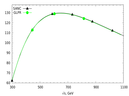
Figure 1: Contribution to the integrated $\sigma_{0}$ cross section. Black line is SANC result, green line is result from paper  [17].

fig01

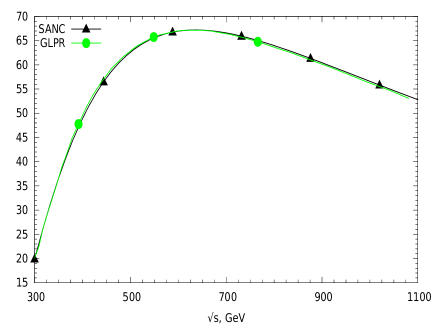
Figure 2: Contribution to the integrated $\sigma_{22}$ cross section. Black line is SANC result, green line is result from paper  [17].

fig02

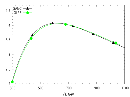
Figure 3: Contribution to the integrated $\sigma_{33}$ cross section. Black line is SANC result, green line is result from paper  [17].

fig03

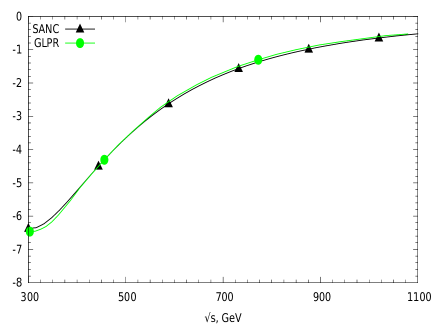
Figure 4: Contribution to the integrated $\sigma_{3}$ cross section. Black line is SANC result, green line is result from paper  [17].

fig04

References

• [1] Ginzburg I.F., Kotkin G.L., Serbo V.G., Telnov V.I. Production of High-Energy Colliding gamma gamma and gamma e Beams with a High Luminosity at Vlepp Accelerators // JETP Lett. —  1981. —  V. 34. —  P. 491–495. —  [Pisma Zh. Eksp. Teor. Fiz.34,514(1981)].
• [2] Ginzburg I.F., Kotkin G.L., Serbo V.G., Telnov V.I. Colliding gamma e and gamma gamma Beams Based on the Single Pass Accelerators (of Vlepp Type) // Nucl. Instrum. Meth. —  1983. —  V. 205. —  P. 47–68.
• [3] Ginzburg I.F., Kotkin G.L., Panfil S.L., Serbo V.G., Telnov V.I. Colliding gamma e and gamma gamma Beams Based on the Single Pass e+ e- Accelerators. 2. Polarization Effects. Monochromatization Improvement // Nucl. Instrum. Meth.A. —  1984. —  V. 219. —  P. 5–24.
• [4] Telnov V.I. Photon collider Higgs factories // JINST. —  2014. —  V. 9, no. 09. —  P. C09020. —  arXiv:1409.5563 [physics.acc-ph].
• [5] Accomando E. et al. [CLIC Physics Working Group Collaboration] Physics at the CLIC multi-TeV linear collider // Proceedings, 11th International Conference on Hadron spectroscopy (Hadron 2005): Rio de Janeiro, Brazil, August 21-26, 2005. —  2004. —  arXiv:hep-ph/0412251.
• [6] Moortgat-Pick G., others. The Role of polarized positrons and electrons in revealing fundamental interactions at the linear collider // Phys. Rept. —  2008. —  V. 460. —  P. 131–243. —  arXiv:hep-ph/0507011.
• [7] Arbey A., others. Physics at the e+ e- Linear Collider // Eur. Phys. J.C. —  2015. —  V. 75, no. 8. —  P. 371. —  arXiv:1504.01726.
• [8] Bardin D., Kalinovskaya L., Uglov E. Standard Model light-by-light scattering in SANC: analytic and numeric evaluation // Phys. Atom. Nucl. —  2010. —  V. 73. —  P. 1878–1888. —  arXiv:0911.5634 [hep-ph].
• [9] Bardin D.Yu., Kalinovskaya L.V., Uglov E.D. $Z\gamma\gamma\gamma\to 0$ processes in SANC // Phys. Atom. Nucl. —  2013. —  V. 76. —  P. 1339–1344. —  arXiv:1212.3105 [hep-ph].
• [10] Andonov A., Arbuzov A., Bardin D., Bondarenko S., Christova P., Kalinovskaya L., Nanava G., von Schlippe W. SANCscope - v.1.00 // Comput. Phys. Commun. —  2006. —  V. 174. —  P. 481–517. —  [Erratum: Comput. Phys. Commun.177,623(2007)] arXiv:hep-ph/0411186.
• [11] Andonov A., Arbuzov A., Bardin D., Bondarenko S., Christova P., Kalinovskaya L., Kolesnikov V., Sadykov R. Standard SANC Modules // Comput. Phys. Commun. —  2010. —  V. 181. —  P. 305–312. —  arXiv:0812.4207 [physics.comp-ph].
• [12] Bardin D.Y., Passarino G. The standard model in the making: Precision study of the electroweak interactions. —  1999. —  Oxford, UK: Clarendon (1999) 685 p.
• [13] Passarino G., Veltman M. One Loop Corrections for e+ e- Annihilation Into mu+ mu- in the Weinberg Model // Nucl.Phys.B. —  1979. —  V. 160. —  P. 151.
• [14] Vermaseren J.A.M. New features of FORM. —  2000. —  arXiv:math-ph/0010025.
• [15] Vega R., Wudka J. A Covariant method for calculating helicity amplitudes // Phys. Rev.D. —  1996. —  V. 53. —  P. 5286–5292. —  [Erratum: Phys. Rev.D56,6037(1997)] arXiv:hep-ph/9511318.
• [16] Diakonidis T., Gounaris G.J., Layssac J. A FORTRAN code for gamma gamma —> Z Z in SM and MSSM // Eur. Phys. J.C. —  2007. —  V. 50. —  P. 47–52. —  arXiv:hep-ph/0610085.
• [17] Gounaris G.J., Layssac J., Porfyriadis P., Renard F.M. The gamma gamma —> Z Z process and the search for virtual SUSY effects at a gamma gamma collider // Eur. Phys. J.C. —  2000. —  V. 13. —  P. 79–97. —  arXiv:hep-ph/9909243.
Refer to caption