Machine learning approximation algorithms
for high-dimensional fully nonlinear partial
differential equations and second-order
backward stochastic differential equations

Abstract

High-dimensional partial differential equations (PDE) appear in a number of models from the financial industry, such as in derivative pricing models, credit valuation adjustment (CVA) models, or portfolio optimization models. The PDEs in such applications are high-dimensional as the dimension corresponds to the number of financial assets in a portfolio. Moreover, such PDEs are often fully nonlinear due to the need to incorporate certain nonlinear phenomena in the model such as default risks, transaction costs, volatility uncertainty (Knightian uncertainty), or trading constraints in the model. Such high-dimensional fully nonlinear PDEs are exceedingly difficult to solve as the computational effort for standard approximation methods grows exponentially with the dimension. In this work we propose a new method for solving high-dimensional fully nonlinear second-order PDEs. Our method can in particular be used to sample from high-dimensional nonlinear expectations. The method is based on (i) a connection between fully nonlinear second-order PDEs and second-order backward stochastic differential equations (2BSDEs), (ii) a merged formulation of the PDE and the 2BSDE problem, (iii) a temporal forward discretization of the 2BSDE and a spatial approximation via deep neural nets, and (iv) a stochastic gradient descent-type optimization procedure. Numerical results obtained using TensorFlow in Python illustrate the efficiency and the accuracy of the method in the cases of a $100$-dimensional Black-Scholes-Barenblatt equation, a $100$-dimensional Hamilton-Jacobi-Bellman equation, and a nonlinear expectation of a $100$-dimensional $G$-Brownian motion.

1 Introduction

Partial differential equations (PDE) play an important role in an abundance of models from finance to physics. Objects as the wave function associated to a quantum physical system, the value function describing the fair price of a financial derivative in a pricing model, or the value function describing the expected maximal utility in a portfolio optimization problem are often given as solutions to nonlinear PDEs. Roughly speaking, the nonlinearities in the above mentioned PDEs from financial engineering applications appear due to certain nonlinear effects in the trading portfolio (the trading portfolio for hedging the financial derivative claim in the case of derivative pricing problems and the trading portfolio whose utility has to be maximized in the case of portfolio optimization problems); see, e.g., [7, 9, 37, 45, 66, 71] for derivative pricing models with different interest rates for borrowing and lending, see, e.g., [24, 53] for derivative pricing models incorporating the default risk of the issuer of the financial derivative, see, e.g., [4, 5, 109] for models for the pricing of financial derivatives on untradable underlyings such as financial derivatives on the temperature or mortality-dependent financial derivatives, see, e.g., [1, 36, 83] for models incorporating that the trading strategy influences the price processes though demand and supply (so-called large investor effects), see, e.g., [39, 50, 70, 94] for models taking transaction costs in the trading portfolio into account, and see, e.g., [2, 50] for models incorporating uncertainties in the model parameters for the underlyings (Knightian uncertainty). The PDEs emerging from such models are often high-dimensional as the associated trading portfolios frequently contain a whole basket of financial assets (see, e.g., [7, 24, 39]). These high-dimensional nonlinear PDEs are typically exceedingly difficult to solve approximatively. Nonetheless, there is a strong demand from the financial engineering industry to approximatively compute the solutions of such high-dimensional nonlinear parabolic PDEs due to the above mentioned practical relevance of these PDEs.

There are a number of numerical methods for solving nonlinear parabolic PDEs approximatively in the literature. Some of these methods are deterministic approximation methods and others are random approximation methods which rely on suitable probabilistic representations of the corresponding PDE solutions such as probabilistic representations based on backward stochastic differential equations (BSDEs) (cf., e.g., [10, 11, 42, 85, 86, 87, 88]), probabilistic representations based on second-order backward stochastic differential equations (2BSDEs) (cf., e.g., [22]), probabilistic representations based on branching diffusions (cf., e.g., [53, 54, 55, 77, 102, 108]), and probabilistic representations based on extensions of the classical Feynman-Kac formula (cf., e.g., [34, 58, 84]). We refer, e.g., to [23, 30, 65, 69, 95, 103, 104, 106] for deterministic approximation methods for PDEs, to [3, 6, 7, 13, 18, 19, 20, 21, 25, 26, 27, 28, 31, 32, 43, 44, 45, 46, 47, 48, 56, 64, 71, 72, 73, 74, 75, 81, 82, 93, 98, 99, 100, 105, 111] for probabilistic approximation methods for PDEs based on temporal discretizations of BSDEs, to [33, 52] for probabilistic approximation methods for PDEs based on suitable deep learning approximations for BSDEs, to [40, 110] for probabilistic approximation methods for BSDEs based on sparse grid approximations, to [14, 41] for probabilistic approximation methods for BSDEs based on Wiener Chaos expansions, to [12, 22, 38, 49, 62, 112] for probabilistic approximation methods for PDEs based on temporal discretization of 2BSDEs, to [17, 53, 54, 55, 96, 107] for probabilistic approximation methods for PDEs based on branching diffusion representations, and to [34, 35] for probabilistic approximation methods based on extensions of the classical Feynman-Kac formula.

Most of the above named approximation methods are, however, only applicable in the case where the PDE/BSDE dimension $d$ is rather small or work exclusively in the case of serious restrictions on the parameters or the type of the considered PDE (e.g., small nonlinearities, small terminal/initial conditions, semilinear structure of the PDE). The numerical solution of a high-dimensional nonlinear PDE thus remains an exceedingly difficult task and there is only a limited number of situations where practical algorithms for high-dimensional PDEs have been developed (cf., e.g., [29, 33, 34, 35, 52, 54, 55, 101]). In particular, to the best of our knowledge, at the moment there exists no practical algorithm for high-dimensional fully nonlinear parabolic PDEs in the scientific literature.

In this work we intend to overcome this difficulty, that is, we propose a new algorithm for solving fully-nonlinear PDEs and nonlinear second-order backward stochastic differential equations 2BSDEs. Our method in particular can be used to sample from Shige Peng’s nonlinear expectation in high space-dimensions (cf., e.g., [89, 90, 91, 92]). The proposed algorithm exploits a connection between PDEs and 2BSDEs (cf., e.g., Cheridito et al. [22]) to obtain a merged formulation of the PDE and the 2BSDE, whose solution is then approximated by combining a time-discretization with a neural network based deep learning procedure (cf., e.g., [8, 15, 16, 23, 30, 33, 51, 52, 59, 63, 65, 68, 67, 69, 78, 79, 95, 97]). Roughly speaking, the merged formulation allows us to formulate the original PDE problem as a learning problem. The random loss function for the deep neural network in our algorithm is, loosely speaking, given by the error between the prescribed terminal condition of the 2BSDE and the neural network based forward time discretization of the 2BSDE. A related deep learning approximation algorithm for PDEs of semilinear type based on forward BSDEs has been recently proposed in [33, 52]. A key difference between [33, 52] and the present work is that here we rely on the connection between fully nonlinear PDEs and 2BSDEs given by Cheridito et al. [22] while [33, 52] rely on the nowadays almost classical connection between PDEs and BSDEs (cf., e.g., [86, 85, 87, 88]). This is the reason why the method proposed in [33, 52] is only applicable to semilinear PDEs while the algorithm proposed here allows to treat fully nonlinear PDEs and nonlinear expectations.

The remainder of this article is organized as follows. In Section 2 we derive (see Subsections 2.1–2.6 below) and formulate (see Subsection 2.7 below) a special case of the algorithm proposed in this work. In Section 3 the proposed algorithm is derived (see Subsections 3.1–3.5 below) and formulated (see Subsection 3.7 below) in the general case. The core idea is most apparent in the simplified framework in Subsection 2.7 (see Framework 2.1 below). The general framework in Subsection 3.7, in turn, allows for employing more sophisticated machine learning techniques (see Framework 3.2 below). In Section 4 we present numerical results for the proposed algorithm in the case of several high-dimensional PDEs. In Subsection 4.1 the proposed algorithm in the simplified framework in Subsection 2.7 is employed to approximatively calculate the solution of a $20$-dimensional Allen-Cahn equation. In Subsections 4.3, 4.4, 4.5, and 4.6 the proposed algorithm in the general framework in Subsection 3.7 is used to approximatively calculate the solution of a $100$-dimensional Black-Scholes-Barenblatt equation, the solution of a $100$-dimensional Hamilton-Jacobi-Bellman equation, the solution of a $50$-dimensional Allen-Cahn equation, and nonlinear expectations of $G$-Brownian motions in $1$ and $100$ space-dimensions. Python implementations of the algorithms are provided in Section A.

2 Main ideas of the deep 2BSDE method

In Subsections 2.1–2.6 below we explain the main idea behind the algorithm proposed in this work which we refer to as deep 2BSDE method. This is done at the expense of a rather sketchy derivation and description. More precise and more general definitions of the deep 2BSDE method may be found in Sections 2.7 and 3.7 below. In a nutshell, the main ingredients of the deep 2BSDE method are

1. a certain connection between PDEs and 2BSDEs,

2. a merged formulation of the PDE and the 2BSDE problem,

3. a temporal forward discretization of the 2BSDE and a spatial approximation via deep neural nets, and

4. a stochastic gradient descent-type optimization procedure.

The derivation of the deep 2BSDE method is mainly based on ideas in E, Han, & Jentzen [33] and Cheridito et al. [22] (cf., e.g., [33, Section 2] and [22, Theorem 4.10]). Let us start now by describing the PDE problems which we want to solve with the deep 2BSDE method.

2.1 Fully nonlinear second-order PDEs

Let $d\in{\mathbb{N}}=\{1,2,3,\ldots\}$, $T\in(0,\infty)$, $u=(u(t,x))_{t\in[0,T],x\in{\mathbb{R}}^{d}}\in C^{1,2}([0,T]\times{\mathbb{R}}^{d},{\mathbb{R}})$, $f\in C([0,T]\times{\mathbb{R}}^{d}\times{\mathbb{R}}\times{\mathbb{R}}^{d}\times{\mathbb{R}}^{d\times d},{\mathbb{R}})$, $g\in C({\mathbb{R}}^{d},{\mathbb{R}})$ satisfy for all $t\in[0,T)$, $x\in{\mathbb{R}}^{d}$ that $u(T,x)=g(x)$ and

$$\tfrac{\partial u}{\partial t}(t,x) =f\bigl{(}t,x,u(t,x),(\nabla_{x}u)(t,x),(\operatorname{Hess}_{x}u)(t,x)\bigr{)}.$$ (1)

The deep 2BSDE method allows us to approximatively compute the function $u(0,x)$, $x\in{\mathbb{R}}^{d}$. To fix ideas we restrict ourselves in this section to the approximative computation of the real number $u(0,\xi)\in{\mathbb{R}}$ for some $\xi\in{\mathbb{R}}^{d}$ and we refer to Subsection 3.7 below for the general algorithm. Moreover, the deep 2BSDE method can easily be extended to the case of systems of fully nonlinear second-order parabolic PDEs but in order to keep the notational complexity as low as possible we restrict ourself to the scalar case in this work (cf. (1) above). Note that the PDE (1) is formulated as a terminal value problem. We chose the terminal value problem formulation over the in the PDE literature more common initial value problem formulation because, on the one hand, the terminal value problem formulation seems to be more natural in connection with second-order BSDEs (which we are going to use below in the derivation of the proposed approximation algorithm) and because, on the other hand, the terminal value problem formulation shows up naturally in financial engineering applications like the Black-Scholes-Barenblatt equation in derivative pricing (cf. Section 4.3). Clearly, terminal value problems can be transformed into initial value problems and vice versa; see, e.g., Remark 3.3 below.

2.2 Connection between fully nonlinear second-order PDEs and 2BSDEs

Let $(\Omega,{\mathcal{F}},\mathbbm{P})$ be a probability space, let $W\colon[0,T]\times\Omega\to{\mathbb{R}}^{d}$ be a standard Brownian motion on $(\Omega,{\mathcal{F}},\mathbbm{P})$ with continuous sample paths, let ${\mathbb{F}}=({\mathbb{F}}_{t})_{t\in[0,T]}$ be the normal filtration on $(\Omega,{\mathcal{F}},\mathbbm{P})$ generated by $W$, and let $Y\colon[0,T]\times\Omega\to{\mathbb{R}}$, $Z\colon[0,T]\times\Omega\to{\mathbb{R}}^{d}$, $\Gamma\colon[0,T]\times\Omega\to{\mathbb{R}}^{d\times d}$, and $A\colon[0,T]\times\Omega\to{\mathbb{R}}^{d}$ be ${\mathbb{F}}$-adapted stochastic processes with continuous sample paths which satisfy that for all $t\in[0,T]$ it holds $\mathbbm{P}$-a.s. that

$$Y_{t}=g(\xi+W_{T})-\int_{t}^{T}\bigl{(}f(s,\xi+W_{s},Y_{s},Z_{s},\Gamma_{s})+\tfrac{1}{2}\operatorname{Trace}(\Gamma_{s})\bigr{)}\,ds-\int_{t}^{T}\langle Z_{s},dW_{s}\rangle_{{\mathbb{R}}^{d}}$$ (2)

and

$$Z_{t}=Z_{0}+\int_{0}^{t}A_{s}\,ds+\int_{0}^{t}\Gamma_{s}\,dW_{s}.$$ (3)

Under suitable smoothness and regularity hypotheses the fully nonlinear PDE (1) is related to the 2BSDE system (2)–(3) in the sense that for all $t\in[0,T]$ it holds $\mathbbm{P}$-a.s. that

$$Y_{t}=u(t,\xi+W_{t})\in{\mathbb{R}},\qquad Z_{t}=(\nabla_{x}u)(t,\xi+W_{t})\in{\mathbb{R}}^{d},$$ (4)

$$\Gamma_{t}=(\operatorname{Hess}_{x}u)(t,\xi+W_{t})\in{\mathbb{R}}^{d\times d},\qquad~{}\text{and}$$ (5)

$$A_{t}=(\tfrac{\partial}{\partial t}\nabla_{x}u)(t,\xi+W_{t})+\tfrac{1}{2}(\nabla_{x}\Delta_{x}u)(t,\xi+W_{t})\in{\mathbb{R}}^{d}$$ (6)

(cf., e.g., Cheridito et al. [22] and Lemma 3.1 below).

2.3 Merged formulation of the PDE and the 2BSDE

In this subsection we derive a merged formulation (see (9) and (10)) for the PDE (1) and the 2BSDE system (2)–(3). More specifically, observe that (2) and (3) yield that for all $\tau_{1},\tau_{2}\in[0,T]$ with $\tau_{1}\leq\tau_{2}$ it holds $\mathbbm{P}$-a.s. that

$$Y_{\tau_{2}}=Y_{\tau_{1}}+\int_{\tau_{1}}^{\tau_{2}}\bigl{(}f(s,\xi+W_{s},Y_{s},Z_{s},\Gamma_{s})+\tfrac{1}{2}\operatorname{Trace}(\Gamma_{s})\bigr{)}\,ds+\int_{\tau_{1}}^{\tau_{2}}\langle Z_{s},dW_{s}\rangle_{{\mathbb{R}}^{d}}$$ (7)

and

$$Z_{\tau_{2}}=Z_{\tau_{1}}+\int_{\tau_{1}}^{\tau_{2}}A_{s}\,ds+\int_{\tau_{1}}^{\tau_{2}}\Gamma_{s}\,dW_{s}.$$ (8)

Putting (5) and (6) into (7) and (8) demonstrates that for all $\tau_{1},\tau_{2}\in[0,T]$ with $\tau_{1}\leq\tau_{2}$ it holds $\mathbbm{P}$-a.s. that

$$\begin{split}&Y_{\tau_{2}}=Y_{\tau_{1}}+\int_{\tau_{1}}^{\tau_{2}}\langle Z_{s},dW_{s}\rangle_{{\mathbb{R}}^{d}}\\ &+\int_{\tau_{1}}^{\tau_{2}}\Bigl{(}f\bigl{(}s,\xi+W_{s},Y_{s},Z_{s},(\operatorname{Hess}_{x}u)(s,\xi+W_{s})\bigr{)}+\tfrac{1}{2}\operatorname{Trace}\bigl{(}(\operatorname{Hess}_{x}u)(s,\xi+W_{s})\bigr{)}\Bigr{)}\,ds\end{split}$$ (9)

and

$$\begin{split}Z_{\tau_{2}}&=Z_{\tau_{1}}+\int_{\tau_{1}}^{\tau_{2}}\bigl{(}(\tfrac{\partial}{\partial t}\nabla_{x}u)(s,\xi+W_{s})+\tfrac{1}{2}(\nabla_{x}\Delta_{x}u)(s,\xi+W_{s})\bigr{)}\,ds\\ &\quad+\int_{\tau_{1}}^{\tau_{2}}(\operatorname{Hess}_{x}u)(s,\xi+W_{s})\,dW_{s}.\end{split}$$ (10)

2.4 Forward-discretization of the merged PDE-2BSDE system

In this subsection we derive a forward-discretization of the merged PDE-2BSDE system (9)–(10). Let $t_{0},t_{1},\ldots,t_{N}\in[0,T]$ be real numbers with

$$0=t_{0}<t_{1}<\ldots<t_{N}=T.$$ (11)

such that the mesh size $\sup_{0\leq k\leq N}(t_{k+1}-t_{k})$ is sufficiently small. Note that (9) and (10) suggest that for sufficiently large $N\in{\mathbb{N}}$ it holds for all $n\in\{0,1,\ldots,N-1\}$ that

$$\begin{split}Y_{t_{n+1}}&\approx Y_{t_{n}}+\Bigl{(}f\bigl{(}t_{n},\xi+W_{t_{n}},Y_{t_{n}},Z_{t_{n}},(\operatorname{Hess}_{x}u)(t_{n},\xi+W_{t_{n}})\bigr{)}\\ &\quad+\tfrac{1}{2}\operatorname{Trace}\bigl{(}(\operatorname{Hess}_{x}u)(t_{n},\xi+W_{t_{n}})\bigr{)}\Bigr{)}(t_{n+1}-t_{n})+\langle Z_{t_{n}},W_{t_{n+1}}-W_{t_{n}}\rangle_{{\mathbb{R}}^{d}}\end{split}$$ (12)

and

$$\begin{split}Z_{t_{n+1}}&\approx Z_{t_{n}}+\bigl{(}(\tfrac{\partial}{\partial t}\nabla_{x}u)(t_{n},\xi+W_{t_{n}})+\tfrac{1}{2}(\nabla_{x}\Delta_{x}u)(t_{n},\xi+W_{t_{n}})\bigr{)}\,(t_{n+1}-t_{n})\\ &\quad+(\operatorname{Hess}_{x}u)(t_{n},\xi+W_{t_{n}})\,(W_{t_{n+1}}-W_{t_{n}}).\end{split}$$ (13)

2.5 Deep learning approximations

In the next step we employ for every $n\in\{0,1,\ldots,N-1\}$ suitable approximations for the functions

$${\mathbb{R}}^{d}\ni x\mapsto(\operatorname{Hess}_{x}u)(t_{n},x)\in{\mathbb{R}}^{d\times d}$$ (14)

and

$${\mathbb{R}}^{d}\ni x\mapsto(\tfrac{\partial}{\partial t}\nabla_{x}u)(t_{n},x)+\tfrac{1}{2}(\nabla_{x}\Delta_{x}u)(t_{n},x)\in{\mathbb{R}}^{d}$$ (15)

in (12)–(13) but not for the functions ${\mathbb{R}}^{d}\ni x\mapsto u(t_{n},x)\in{\mathbb{R}}^{d}$ and ${\mathbb{R}}^{d}\ni x\mapsto(\nabla_{x}u)(t_{n},x)\in{\mathbb{R}}^{d}$ in (4). More precisely, let $\nu\in{\mathbb{N}}\cap[d+1,\infty)$, for every $\theta\in{\mathbb{R}}^{\nu}$, $n\in\{0,1,\ldots,N\}$ let ${\mathbbm{G}}^{\theta}_{n}\colon{\mathbb{R}}^{d}\to{\mathbb{R}}^{d\times d}$ and ${\mathbbm{A}}^{\theta}_{n}\colon{\mathbb{R}}^{d}\to{\mathbb{R}}^{d}$ be continuous functions, and for every $\theta=(\theta_{1},\theta_{2},\ldots,\theta_{\nu})\in{\mathbb{R}}^{\nu}$ let ${\mathcal{Y}}^{\theta}\colon\{0,1,\ldots,N\}\times\Omega\to{\mathbb{R}}$ and ${\mathcal{Z}}^{\theta}\colon\{0,1,\ldots,N\}\times\Omega\to{\mathbb{R}}^{d}$ be stochastic processes which satisfy that ${\mathcal{Y}}^{\theta}_{0}=\theta_{1}$ and ${\mathcal{Z}}^{\theta}_{0}=(\theta_{2},\theta_{3},\ldots,\theta_{d+1})$ and which satisfy for all $n\in\{0,1,\ldots,N-1\}$ that

$$\begin{split}&{\mathcal{Y}}^{\theta}_{n+1}={\mathcal{Y}}^{\theta}_{n}+\langle{\mathcal{Z}}^{\theta}_{n},W_{t_{n+1}}-W_{t_{n}}\rangle_{{\mathbb{R}}^{d}}\\ &+\Bigl{(}f\bigl{(}t_{n},\xi+W_{t_{n}},{\mathcal{Y}}^{\theta}_{n},{\mathcal{Z}}^{\theta}_{n},{\mathbbm{G}}^{\theta}_{n}(\xi+W_{t_{n}})\bigr{)}+\tfrac{1}{2}\operatorname{Trace}\bigl{(}{\mathbbm{G}}^{\theta}_{n}(\xi+W_{t_{n}})\bigr{)}\Bigr{)}\,(t_{n+1}-t_{n})\end{split}$$ (16)

and

$${\mathcal{Z}}^{\theta}_{n+1}={\mathcal{Z}}^{\theta}_{n}+{\mathbbm{A}}^{\theta}_{n}(\xi+W_{t_{n}})\,(t_{n+1}-t_{n})+{\mathbbm{G}}^{\theta}_{n}(\xi+W_{t_{n}})\,(W_{t_{n+1}}-W_{t_{n}}).$$ (17)

For all suitable $\theta\in{\mathbb{R}}^{\nu}$ and all $n\in\{0,1,\ldots,N\}$ we think of ${\mathcal{Y}}^{\theta}_{n}\colon\Omega\to{\mathbb{R}}$ as an appropriate approximation

$${\mathcal{Y}}^{\theta}_{n}\approx Y_{t_{n}}$$ (18)

of $Y_{t_{n}}\colon\Omega\to{\mathbb{R}}$, for all suitable $\theta\in{\mathbb{R}}^{\nu}$ and all $n\in\{0,1,\ldots,N\}$ we think of ${\mathcal{Z}}^{\theta}_{n}\colon\Omega\to{\mathbb{R}}^{d}$ as an appropriate approximation

$${\mathcal{Z}}^{\theta}_{n}\approx Z_{t_{n}}$$ (19)

of $Z_{t_{n}}\colon\Omega\to{\mathbb{R}}^{d}$, for all suitable $\theta\in{\mathbb{R}}^{\nu}$, $x\in{\mathbb{R}}^{d}$ and all $n\in\{0,1,\ldots,N-1\}$ we think of ${\mathbbm{G}}^{\theta}_{n}(x)\in{\mathbb{R}}^{d\times d}$ as an appropriate approximation

$${\mathbbm{G}}^{\theta}_{n}(x)\approx(\operatorname{Hess}_{x}u)(t_{n},x)$$ (20)

of $(\operatorname{Hess}_{x}u)(t_{n},x)\in{\mathbb{R}}^{d\times d},$ and for all suitable $\theta\in{\mathbb{R}}^{\nu}$, $x\in{\mathbb{R}}^{d}$ and all $n\in\{0,1,\ldots,N-1\}$ we think of ${\mathbbm{A}}^{\theta}_{n}(x)\in{\mathbb{R}}^{d}$ as an appropriate approximation

$${\mathbbm{A}}^{\theta}_{n}(x)\approx(\tfrac{\partial}{\partial t}\nabla_{x}u)(t_{n},x)+\tfrac{1}{2}(\nabla_{x}\Delta_{x}u)(t_{n},x)$$ (21)

of $(\tfrac{\partial}{\partial t}\nabla_{x}u)(t_{n},x)+\tfrac{1}{2}(\nabla_{x}\Delta_{x}u)(t_{n},x)\in{\mathbb{R}}^{d}$. In particular, we think of $\theta_{1}$ as an appropriate approximation

$$\theta_{1}\approx u(0,\xi)$$ (22)

of $u(0,\xi)\in{\mathbb{R}},$ and we think of $(\theta_{2},\theta_{3},\ldots,\theta_{d+1})$ as an appropriate approximation

$$(\theta_{2},\theta_{3},\ldots,\theta_{d+1})\approx(\nabla_{x}u)(0,\xi)$$ (23)

of $(\nabla_{x}u)(0,\xi)\in{\mathbb{R}}^{d}$. We suggest for every $n\in\{0,1,\ldots,N-1\}$ to choose the functions ${\mathbbm{G}}^{\theta}_{n}$ and ${\mathbbm{A}}^{\theta}_{n}$ as deep neural networks (cf., e.g., [8, 67]). For example, for every $k\in{\mathbb{N}}$ let $\mathcal{R}_{k}\colon{\mathbb{R}}^{k}\to{\mathbb{R}}^{k}$ be the function which satisfies for all $x=(x_{1},\dots,x_{k})\in{\mathbb{R}}^{k}$ that

$$\mathcal{R}_{k}(x)=\left(\max\{x_{1},0\},\dots,\max\{x_{k},0\}\right),$$ (24)

for every $\theta=(\theta_{1},\dots,\theta_{\nu})\in{\mathbb{R}}^{\nu}$, $v\in{\mathbb{N}}_{0}=\{0\}\cup{\mathbb{N}}$, $k,l\in{\mathbb{N}}$ with $v+k(l+1)\leq\nu$ let $M^{\theta,v}_{k,l}\colon{\mathbb{R}}^{l}\to{\mathbb{R}}^{k}$ be the affine linear function which satisfies for all $x=(x_{1},\dots,x_{l})$ that

$$M^{\theta,v}_{k,l}(x)=\left(\begin{array}[]{cccc}\theta_{v+1}&\theta_{v+2}&\dots&\theta_{v+l}\\ \theta_{v+l+1}&\theta_{v+l+2}&\dots&\theta_{v+2l}\\ \theta_{v+2l+1}&\theta_{v+2l+2}&\dots&\theta_{v+3l}\\ \vdots&\vdots&\vdots&\vdots\\ \theta_{v+(k-1)l+1}&\theta_{v+(k-1)l+2}&\dots&\theta_{v+kl}\end{array}\right)\left(\begin{array}[]{c}x_{1}\\ x_{2}\\ x_{3}\\ \vdots\\ x_{l}\end{array}\right)+\left(\begin{array}[]{c}\theta_{v+kl+1}\\ \theta_{v+kl+2}\\ \theta_{v+kl+3}\\ \vdots\\ \theta_{v+kl+k}\end{array}\right),$$ (25)

assume that $\nu\geq(5Nd+Nd^{2}+1)(d+1)$, and assume for all $\theta\in{\mathbb{R}}^{\nu}$, $n\in\{m\in{\mathbb{N}}\colon m<N\}$, $x\in{\mathbb{R}}^{d}$ that

$${\mathbbm{A}}^{\theta}_{n}=M^{\theta,[(2N+n)d+1](d+1)}_{d,d}\circ\mathcal{R}_{d}\circ M^{\theta,[(N+n)d+1](d+1)}_{d,d}\\ \circ\mathcal{R}_{d}\circ M^{\theta,(nd+1)(d+1)}_{d,d}$$ (26)

and

$${\mathbbm{G}}^{\theta}_{n}=M^{\theta,(5Nd+nd^{2}+1)(d+1)}_{d^{2},d}\circ\mathcal{R}_{d}\circ M^{\theta,[(4N+n)d+1](d+1)}_{d,d}\circ\mathcal{R}_{d}\circ M^{\theta,[(3N+n)d+1](d+1)}_{d,d}.$$ (27)

The functions in (26) provide artifical neural networks with $4$ layers ($1$ input layer with $d$ neurons, $2$ hidden layers with $d$ neurons each, and $1$ output layer with $d$ neurons) and rectifier functions as activation functions (see (24)). The functions in (27) also provide artificial neural networks with $4$ layers ($1$ input layer with $d$ neurons, $2$ hidden layers with $d$ neurons each, and $1$ output layer with $d^{2}$ neurons) and rectifier functions as activation functions (see (24)).

2.6 Stochastic gradient descent-type optimization

We intend to reach a suitable $\theta\in{\mathbb{R}}^{\nu}$ in (18)–(23) by applying a stochastic gradient descent-type minimization algorithm to the function

$${\mathbb{R}}^{\nu}\ni\theta\mapsto{\mathbbm{E}}\big{[}|{\mathcal{Y}}^{\theta}_{N}-g(\xi+W_{t_{N}})|^{2}\big{]}\in{\mathbb{R}}.$$ (28)

Minimizing the function in (28) is inspired by the fact that

$${\mathbbm{E}}[|Y_{T}-g(\xi+W_{T})|^{2}]=0$$ (29)

according to (2). Applying a stochastic gradient descent-type minimization algorithm yields under suitable assumptions random approximations

$$\Theta_{m}=(\Theta_{m}^{(1)},\Theta_{m}^{(2)},\ldots,\Theta_{m}^{(\nu)})\colon\Omega\to{\mathbb{R}}^{\nu}$$ (30)

for $m\in{\mathbb{N}}_{0}$ of a local minimum point of the function in (28). For sufficiently large $N,\nu,m\in{\mathbb{N}}$ we use the random variable $\Theta_{m}^{(1)}\colon\Omega\to{\mathbb{R}}$ as an appropriate approximation

$$\Theta_{m}^{(1)}\approx u(0,\xi)$$ (31)

of $u(0,\xi)\in{\mathbb{R}}$ (cf. (22) above). In the next subsection the proposed algorithm is described in more detail.

2.7 Framework for the algorithm in a specific case

In this subsection we describe the deep 2BSDE method in the specific case where (1) is the PDE under consideration, where the standard Euler-Maruyama scheme (cf., e.g., [61, 76, 80]) is the employed approximation scheme for discretizing (9) and (10) (cf. (16) and (17)), and where the plain stochastic gradient descent with constant learning rate $\gamma\in(0,\infty)$ is the employed minimization algorithm. A more general description of the deep 2BSDE method, which allows to incorporate more sophisticated machine learning approximation techniques such as batch normalization or the Adam optimizer, can be found in Subsection 3.7 below.

Framework 2.1 (Special case).

Let $T,\gamma\in(0,\infty)$, $d,N\in{\mathbb{N}}$, $\nu\in{\mathbb{N}}\cap[d+1,\infty)$, $\xi\in{\mathbb{R}}^{d}$, let $f\colon[0,T]\times{\mathbb{R}}^{d}\times{\mathbb{R}}\times{\mathbb{R}}^{d}\times{\mathbb{R}}^{d\times d}\to{\mathbb{R}}$ and $g\colon{\mathbb{R}}^{d}\to{\mathbb{R}}$ be functions, let $(\Omega,{\mathcal{F}},\mathbbm{P})$ be a probability space, let $W^{m}\colon[0,T]\times\Omega\to{\mathbb{R}}^{d}$, $m\in{\mathbb{N}}_{0}$, be independent standard Brownian motions on $(\Omega,{\mathcal{F}},\mathbbm{P})$, let $t_{0},t_{1},\ldots,t_{N}\in[0,T]$ be real numbers with $0=t_{0}<t_{1}<\ldots<t_{N}=T$, for every $\theta\in{\mathbb{R}}^{\nu}$, $n\in\{0,1,\ldots,N-1\}$ let ${\mathbbm{A}}_{n}^{\theta}\colon{\mathbb{R}}^{d}\to{\mathbb{R}}^{d}$ and ${\mathbbm{G}}_{n}^{\theta}\colon{\mathbb{R}}^{d}\to{\mathbb{R}}^{d\times d}$ be functions, for every $m\in{\mathbb{N}}_{0}$, $\theta\in{\mathbb{R}}^{\nu}$ let ${\mathcal{Y}}^{m,\theta}\colon\{0,1,\ldots,N\}\times\Omega\to{\mathbb{R}}$ and ${\mathcal{Z}}^{m,\theta}\colon\{0,1,\ldots,N\}\times\Omega\to{\mathbb{R}}^{d}$ be stochastic processes which satisfy that ${\mathcal{Y}}^{m,\theta}_{0}=\theta_{1}$ and ${\mathcal{Z}}^{m,\theta}_{0}=(\theta_{2},\theta_{3},\ldots,\theta_{d+1})$ and which satisfy for all $n\in\{0,1,\ldots,N-1\}$ that

$$\begin{split}&{\mathcal{Y}}^{m,\theta}_{n+1}={\mathcal{Y}}^{m,\theta}_{n}+\langle{\mathcal{Z}}^{m,\theta}_{n},W^{m}_{t_{n+1}}-W^{m}_{t_{n}}\rangle_{{\mathbb{R}}^{d}}\\ &+\Bigl{(}f\bigl{(}t_{n},\xi+W^{m}_{t_{n}},{\mathcal{Y}}^{m,\theta}_{n},{\mathcal{Z}}^{m,\theta}_{n},{\mathbbm{G}}^{\theta}_{n}(\xi+W^{m}_{t_{n}})\bigr{)}+\tfrac{1}{2}\operatorname{Trace}\bigl{(}{\mathbbm{G}}^{\theta}_{n}(\xi+W^{m}_{t_{n}})\bigr{)}\Bigr{)}(t_{n+1}-t_{n})\end{split}$$ (32)

$$\text{and}\qquad{\mathcal{Z}}^{m,\theta}_{n+1}={\mathcal{Z}}^{m,\theta}_{n}+{\mathbbm{A}}^{\theta}_{n}(\xi+W^{m}_{t_{n}})\,(t_{n+1}-t_{n})+{\mathbbm{G}}^{\theta}_{n}(\xi+W^{m}_{t_{n}})\,(W^{m}_{t_{n+1}}-W^{m}_{t_{n}}),$$ (33)

for every $m\in{\mathbb{N}}_{0}$ let $\phi^{m}\colon{\mathbb{R}}^{\nu}\times\Omega\to{\mathbb{R}}$ be the function which satisfies for all $\theta\in{\mathbb{R}}^{\nu}$, $\omega\in\Omega$ that

$$\phi^{m}(\theta,\omega)=\bigl{|}{\mathcal{Y}}^{m,\theta}_{N}(\omega)-g\bigl{(}\xi+W^{m}_{T}(\omega)\bigr{)}\bigr{|}^{2},$$ (34)

for every $m\in{\mathbb{N}}_{0}$ let $\Phi^{m}\colon{\mathbb{R}}^{\nu}\times\Omega\to{\mathbb{R}}^{\nu}$ be a function which satisfies for all $\omega\in\Omega$, $\theta\in\{\eta\in{\mathbb{R}}^{\nu}\colon~{}\phi^{m}(\cdot,\omega)\colon{\mathbb{R}}^{\nu}\to{\mathbb{R}}~{}\text{is differentiable at}~{}\eta\}$ that

$$\Phi^{m}(\theta,\omega)=(\nabla_{\theta}\phi^{m})(\theta,\omega),$$ (35)

and let $\Theta=(\Theta^{(1)},\dots,\Theta^{(\nu)})\colon{\mathbb{N}}_{0}\times\Omega\to{\mathbb{R}}^{\nu}$ be a stochastic process which satisfies for all $m\in{\mathbb{N}}_{0}$ that

$$\Theta_{m+1}=\Theta_{m}-\gamma\cdot\Phi^{m}(\Theta_{m}).$$ (36)

Under suitable further assumptions, we think in the case of sufficiently large $N,\nu\in{\mathbb{N}}$, $m\in{\mathbb{N}}_{0}$ and sufficiently small $\gamma\in(0,\infty)$ in Framework 2.1 of the random variable $\Theta_{m}=(\Theta_{m}^{(1)},\ldots,\Theta_{m}^{(\nu)})\colon\Omega\to{\mathbb{R}}^{\nu}$ as an appropriate approximation of a local minimum point of the expected loss function and we think in the case of sufficiently large $N,\nu\in{\mathbb{N}}$, $m\in{\mathbb{N}}_{0}$ and sufficiently small $\gamma\in(0,\infty)$ in Framework 2.1 of the random variable $\Theta_{m}^{(1)}\colon\Omega\to{\mathbb{R}}$ as an appropriate approximation of the value $u(0,\xi)\in{\mathbb{R}}$ where $u\colon[0,T]\times{\mathbb{R}}^{d}\to{\mathbb{R}}$ is an at most polynomially growing continuous function which satisfies for all $(t,x)\in[0,T)\times{\mathbb{R}}^{d}$ that $u|_{[0,T)\times{\mathbb{R}}^{d}}\in C^{1,2}([0,T)\times{\mathbb{R}}^{d},{\mathbb{R}})$, $u(T,x)=g(x)$, and

$$\tfrac{\partial u}{\partial t}(t,x)=f\bigl{(}t,x,u(t,x),(\nabla_{x}u)(t,x),(\operatorname{Hess}_{x}u)(t,x)\bigr{)}.$$ (37)

In Subsection 4.1 below an implementation of Framework 2.1 (see Python code 1 in Appendix A.1 below) is employed to calculate numerical approximations for the Allen-Cahn equation in $20$ space-dimensions ($d=20$). In Subsection 4.5 below numerical approximations for the Allen-Cahn equation in $50$ space-dimensions are calculated by means of the algorithm in the more general setting in Framework 3.2 below.

3 The deep 2BSDE method in the general case

In this section we extend and generalize the approximation scheme derived and presented in Section 2. The core idea of the approximation scheme in this section remains the same as in Section 2 but, in contrast to Section 2, in this section the background dynamics in the approximation scheme may be a more general Itô process than just a Brownian motion (cf. Lemma 3.1 in Subsection 3.2 below) and, in contrast to Section 2, in this section the approximation scheme may employ more sophisticated machine learning techniques (cf. Framework 3.2 in Subsection 3.7 below).

3.1 Fully nonlinear second-order PDEs

Let $d\in{\mathbb{N}}$, $T\in(0,\infty)$, let $u=(u(t,x))_{t\in[0,T],x\in{\mathbb{R}}^{d}}\in C^{1,2}([0,T]\times{\mathbb{R}}^{d},{\mathbb{R}})$, $f\colon[0,T]\times{\mathbb{R}}^{d}\times{\mathbb{R}}\times{\mathbb{R}}^{d}\times{\mathbb{R}}^{d\times d}\to{\mathbb{R}}$, and $g\colon[0,T]\times{\mathbb{R}}^{d}\to{\mathbb{R}}$ be functions which satisfy for all $(t,x)\in[0,T)\times{\mathbb{R}}^{d}$ that $u(T,x)=g(x)$ and

$$\tfrac{\partial u}{\partial t}(t,x)=f\bigl{(}t,x,u(t,x),(\nabla_{x}u)(t,x),(\operatorname{Hess}_{x}u)(t,x)\bigr{)}.$$ (38)

Our goal is to approximatively compute the solution $u$ of the PDE (38) at time $t=0$, that is, our goal is to approximatively calculate the function ${\mathbb{R}}^{d}\ni x\mapsto u(0,x)\in{\mathbb{R}}$. For this, we make use of the following connection between fully nonlinear second-order PDEs and second-order BSDEs.

3.2 Connection between fully nonlinear second-order PDEs and 2BSDEs

The deep 2BSDE method relies on a connection between fully nonlinear second-order PDEs and second-order BSDEs; cf., e.g., Theorem 4.10 in Cheridito et al. [22] and Lemma 3.1 below.

Lemma 3.1 (Cf., e.g., Section 3 in Cheridito et al. [22]).

Let $d\in{\mathbb{N}}$, $T\in(0,\infty)$, let $u=(u(t,x))_{t\in[0,T],x\in{\mathbb{R}}^{d}}\in C^{1,2}([0,T]\times{\mathbb{R}}^{d},{\mathbb{R}})$, $\mu\in C({\mathbb{R}}^{d},{\mathbb{R}}^{d})$, $\sigma\in C({\mathbb{R}}^{d},{\mathbb{R}}^{d\times d})$, $f\colon[0,T]\times{\mathbb{R}}^{d}\times{\mathbb{R}}\times{\mathbb{R}}^{d}\times{\mathbb{R}}^{d\times d}\to{\mathbb{R}}$, and $g\colon{\mathbb{R}}^{d}\to{\mathbb{R}}$ be functions which satisfy for all $t\in[0,T)$, $x\in{\mathbb{R}}^{d}$ that $\nabla_{x}u\in C^{1,2}([0,T]\times{\mathbb{R}}^{d},{\mathbb{R}}^{d})$, $u(T,x)=g(x)$, and

$$\tfrac{\partial u}{\partial t}(t,x) =f\bigl{(}t,x,u(t,x),(\nabla_{x}u)(t,x),(\operatorname{Hess}_{x}u)(t,x)\bigr{)},$$ (39)

let $(\Omega,{\mathcal{F}},\mathbbm{P})$ be a probability space, let $W=(W^{(1)},\dots,W^{(d)})\colon[0,T]\times\Omega\to{\mathbb{R}}^{d}$ be a standard Brownian motion on $(\Omega,{\mathcal{F}},\mathbbm{P})$, let ${\mathbb{F}}=({\mathbb{F}}_{t})_{t\in[0,T]}$ be the normal filtration on $(\Omega,{\mathcal{F}},\mathbbm{P})$ generated by $W$, let $\xi\colon\Omega\to{\mathbb{R}}^{d}$ be an ${\mathcal{F}}_{0}/\mathcal{B}({\mathbb{R}}^{d})$-measurable function, let $X=(X^{(1)},\ldots,X^{(d)})\colon[0,T]\times\Omega\to{\mathbb{R}}^{d}$ be an ${\mathbb{F}}$-adapted stochastic process with continuous sample paths which satisfies that for all $t\in[0,T]$ it holds $\mathbbm{P}$-a.s. that

$$X_{t}=\xi+\int_{0}^{t}\mu(X_{s})\,ds+\int_{0}^{t}\sigma(X_{s})\,dW_{s},$$ (40)

for every $\varphi\in C^{1,2}([0,T]\times{\mathbb{R}}^{d},{\mathbb{R}})$ let ${\mathcal{L}}\varphi\colon[0,T]\times{\mathbb{R}}^{d}\to{\mathbb{R}}$ be the function which satisfies for all $(t,x)\in[0,T]\times{\mathbb{R}}^{d}$ that

$$({\mathcal{L}}\varphi)(t,x)=(\tfrac{\partial\varphi}{\partial t})(t,x)+\tfrac{1}{2}\operatorname{Trace}\bigl{(}\sigma(x)\sigma(x)^{\ast}(\operatorname{Hess}_{x}\varphi)(t,x)\bigr{)},$$ (41)

and let $Y\colon[0,T]\times\Omega\to{\mathbb{R}}$, $Z=(Z^{(1)},\ldots,Z^{(d)})\colon[0,T]\times\Omega\to{\mathbb{R}}^{d}$, $\Gamma=(\Gamma^{(i,j)})_{(i,j)\in\{1,\ldots,d\}^{2}}\colon[0,T]\times\Omega\to{\mathbb{R}}^{d\times d}$, and $A=(A^{(1)},\ldots,A^{(d)})\colon[0,T]\times\Omega\to{\mathbb{R}}^{d}$ be the stochastic processes which satisfy for all $t\in[0,T]$, $i\in\{1,2,\ldots,d\}$ that

$$Y_{t}=u(t,X_{t}),\quad Z_{t}=(\nabla_{x}u)(t,X_{t}),\quad\Gamma_{t}=(\operatorname{Hess}_{x}u)(t,X_{t}),\quad A_{t}^{(i)}=({\mathcal{L}}(\tfrac{\partial u}{\partial x_{i}}))(t,X_{t}).$$ (42)

Then it holds that $Y$, $Z$, $\Gamma$, and $A$ are ${\mathbb{F}}$-adapted stochastic processes with continuous sample paths which satisfy that for all $t\in[0,T]$ it holds $\mathbbm{P}$-a.s. that

$$Y_{t}=g(X_{T})-\int_{t}^{T}\bigl{(}f(s,X_{s},Y_{s},Z_{s},\Gamma_{s})+\tfrac{1}{2}\operatorname{Trace}(\sigma(X_{s})\sigma(X_{s})^{\ast}\Gamma_{s})\bigr{)}\,ds-\int_{t}^{T}\langle Z_{s},dX_{s}\rangle_{{\mathbb{R}}^{d}}$$ (43)

and

$$Z_{t}=Z_{0}+\int_{0}^{t}A_{s}\,ds+\int_{0}^{t}\Gamma_{s}\,dX_{s}.$$ (44)

Proof of Lemma 3.1.

Note that $u\colon[0,T]\times{\mathbb{R}}^{d}\to{\mathbb{R}}$, $\nabla_{x}u\colon[0,T]\times{\mathbb{R}}^{d}\to{\mathbb{R}}^{d}$, $\operatorname{Hess}_{x}u\colon[0,T]\times{\mathbb{R}}^{d}\to{\mathbb{R}}^{d\times d}$, and $\bigl{(}{\mathcal{L}}\tfrac{\partial u}{\partial x_{i}}\bigr{)}\colon[0,T]\times{\mathbb{R}}^{d}\to{\mathbb{R}}$, $i\in\{1,2,\ldots,d\}$, are continuous functions. Combining this and (42) with the continuity of the sample paths of $X$ shows that $Y$, $Z$, $\Gamma$, and $A$ are ${\mathbb{F}}$-adapted stochastic process with continuous sample paths. Next observe that Itô’s lemma and the assumption that $u\in C^{1,2}([0,T]\times{\mathbb{R}}^{d},{\mathbb{R}})$ yield that for all $r\in[0,T]$ it holds $\mathbbm{P}$-a.s. that

$$\begin{split}u(T,X_{T})&=u(r,X_{r})+\int_{r}^{T}\langle(\nabla_{x}u)(s,X_{s}),dX_{s}\rangle_{{\mathbb{R}}^{d}}\\ &\quad+\int_{r}^{T}\Bigl{(}(\tfrac{\partial u}{\partial t})(s,X_{s})+\tfrac{1}{2}\operatorname{Trace}\bigl{(}\sigma(X_{s})\sigma(X_{s})^{\ast}(\operatorname{Hess}_{x}u)(s,X_{s})\bigr{)}\Bigr{)}\,ds.\end{split}$$ (45)

This, (39), and (42) yield that for all $r\in[0,T]$ it holds $\mathbbm{P}$-a.s. that

$$\begin{split}g(X_{T})&=Y_{r}+\int_{r}^{T}\langle Z_{s},dX_{s}\rangle_{{\mathbb{R}}^{d}}\\ &\quad+\int_{r}^{T}\Bigl{(}f(s,X_{s},Y_{s},Z_{s},\Gamma_{s})+\tfrac{1}{2}\operatorname{Trace}\bigl{(}\sigma(X_{s})\sigma(X_{s})^{\ast}\Gamma_{s}\bigr{)}\Bigr{)}\,ds.\end{split}$$ (46)

This establishes (43). In the next step we note that Itô’s lemma and the hypothesis that $\nabla_{x}u=(\frac{\partial u}{\partial x_{1}},\dots,\frac{\partial u}{\partial x_{d}})\in C^{1,2}([0,T]\times{\mathbb{R}}^{d},{\mathbb{R}}^{d})$ guarantee that for all $i\in\{1,2,\ldots,d\}$, $r\in[0,T]$ it holds $\mathbbm{P}$-a.s. that

$$\begin{split}(\tfrac{\partial u}{\partial x_{i}})(r,X_{r})&=(\tfrac{\partial u}{\partial x_{i}})(0,X_{0})+\int_{0}^{r}\langle(\nabla_{x}\tfrac{\partial u}{\partial x_{i}})(s,X_{s}),\,dX_{s}\rangle_{{\mathbb{R}}^{d}}\\ &\quad+\int_{0}^{r}\Bigl{(}(\tfrac{\partial}{\partial t}\tfrac{\partial u}{\partial x_{i}})(s,X_{s})+\tfrac{1}{2}\operatorname{Trace}\bigl{(}\sigma(X_{s})\sigma(X_{s})^{\ast}(\operatorname{Hess}_{x}\tfrac{\partial u}{\partial x_{i}})(s,X_{s})\bigr{)}\Bigr{)}\,ds.\end{split}$$ (47)

This, (41), and (42) yield that for all $i\in\{1,2,\ldots,d\}$, $r\in[0,T]$ it holds $\mathbbm{P}$-a.s. that

$$\begin{split}Z^{(i)}_{r}&=Z^{(i)}_{0}+\sum_{j=1}^{d}\int_{0}^{r}(\tfrac{\partial}{\partial x_{j}}\tfrac{\partial u}{\partial x_{i}})(s,X_{s})\,dX^{(j)}_{s}\\ &\quad+\int_{0}^{r}\Bigl{(}(\tfrac{\partial}{\partial t}\tfrac{\partial u}{\partial x_{i}})(s,X_{s})+\tfrac{1}{2}\operatorname{Trace}\bigl{(}\sigma(X_{s})\sigma(X_{s})^{\ast}(\operatorname{Hess}_{x}\tfrac{\partial u}{\partial x_{i}})(s,X_{s})\bigr{)}\Bigr{)}\,ds\\ &=Z^{(i)}_{0}+\int_{0}^{r}A^{(i)}_{s}\,ds+\sum_{j=1}^{d}\int_{0}^{r}\Gamma^{(i,j)}_{s}\,dX^{(j)}_{s}.\end{split}$$ (48)

This shows (44). The proof of Lemma 3.1 is thus completed. ∎

In Subsection 2.2 above we have employed Lemma 3.1 in the specific situation where $\forall\,x\in{\mathbb{R}}^{d}\colon\mu(x)=0\in{\mathbb{R}}^{d}$ and $\forall\,x\in{\mathbb{R}}^{d}\colon\sigma(x)=\operatorname{Id}_{{\mathbb{R}}^{d}}\in{\mathbb{R}}^{d\times d}$ (cf. (2)–(6) in Subsection 2.2 and (43)–(44) in Lemma 3.1). In the following we proceed with the merged formulation, the forward-discretization of the merged PDE-2BSDE system, and deep learning approximations similar as in Section 2.

3.3 Merged formulation of the PDE and the 2BSDE

In this subsection we derive a merged formulation (see (55) and (56)) for the PDE (38) and the 2BSDE system (53)–(54) as in Subsection 2.3. To derive the merged formulation of the PDE and the 2BSDE, we employ the following hypotheses in addition to the assumptions in Subsection 3.1 above (cf. Lemma 3.1 above). Let $\mu\colon{\mathbb{R}}^{d}\to{\mathbb{R}}^{d}$ and $\sigma\colon{\mathbb{R}}^{d}\to{\mathbb{R}}^{d\times d}$ be continuous functions, let $(\Omega,{\mathcal{F}},\mathbbm{P})$ be a probability space, let $W\colon[0,T]\times\Omega\to{\mathbb{R}}^{d}$ be a standard Brownian motion on $(\Omega,{\mathcal{F}},\mathbbm{P})$, let ${\mathbb{F}}=({\mathbb{F}}_{t})_{t\in[0,T]}$ be the normal filtration on $(\Omega,{\mathcal{F}},\mathbbm{P})$ generated by $W$, let $\xi\colon\Omega\to{\mathbb{R}}^{d}$ be an ${\mathcal{F}}_{0}/\mathcal{B}({\mathbb{R}}^{d})$-measurable function, let $X=(X^{(1)},\ldots,X^{(d)})\colon[0,T]\times\Omega\to{\mathbb{R}}^{d}$ be an ${\mathbb{F}}$-adapted stochastic process with continuous sample paths which satisfies that for all $t\in[0,T]$ it holds $\mathbbm{P}$-a.s. that

$$X_{t}=\xi+\int_{0}^{t}\mu(X_{s})\,ds+\int_{0}^{t}\sigma(X_{s})\,dW_{s},$$ (49)

let $e^{(d)}_{1}=(1,0,\dots,0)$, $e^{(d)}_{2}=(0,1,0,\dots,0)$, $\dots$, $e^{(d)}_{d}=(0,\dots,0,1)\in{\mathbb{R}}^{d}$ be the standard basis vectors of ${\mathbb{R}}^{d}$, for every $\varphi\in C^{1,2}([0,T]\times{\mathbb{R}}^{d},{\mathbb{R}}^{d})$ let ${\mathcal{L}}\varphi\colon[0,T]\times{\mathbb{R}}^{d}\to{\mathbb{R}}^{d}$ be the function which satisfies for all $(t,x)\in[0,T]\times{\mathbb{R}}^{d}$ that

$$({\mathcal{L}}\varphi)(t,x)=\tfrac{\partial\varphi}{\partial t}(t,x)+\tfrac{1}{2}\textstyle\sum\limits_{i=1}^{d}\big{(}\tfrac{\partial^{2}\varphi}{\partial x^{2}}\big{)}(t,x)\big{(}\sigma(x)e^{(d)}_{i},\sigma(x)e^{(d)}_{i}\big{)}$$ (50)

and let $Y\colon[0,T]\times\Omega\to{\mathbb{R}}$, $Z\colon[0,T]\times\Omega\to{\mathbb{R}}^{d}$, $\Gamma\colon[0,T]\times\Omega\to{\mathbb{R}}^{d\times d}$, and $A\colon[0,T]\times\Omega\to{\mathbb{R}}^{d}$ be the stochastic processes which satisfy for all $t\in[0,T]$ that

$$Y_{t}=u(t,X_{t}),\quad Z_{t}=(\nabla_{x}u)(t,X_{t}),\quad\Gamma_{t}=(\operatorname{Hess}_{x}u)(t,X_{t}),\quad A_{t}=({\mathcal{L}}(\nabla_{x}u))(t,X_{t}).$$ (51)

Lemma 3.1 implies that for all $\tau_{1},\tau_{2}\in[0,T]$ with $\tau_{1}\leq\tau_{2}$ it holds $\mathbbm{P}$-a.s. that

$$X_{\tau_{2}}=X_{\tau_{1}}+\int_{\tau_{1}}^{\tau_{2}}\mu(X_{s})\,ds+\int_{\tau_{1}}^{\tau_{2}}\sigma(X_{s})\,dW_{s},$$ (52)

$$Y_{\tau_{2}}=Y_{\tau_{1}}+\int_{\tau_{1}}^{\tau_{2}}\bigl{(}f(s,X_{s},Y_{s},Z_{s},\Gamma_{s})+\tfrac{1}{2}\text{Trace}(\sigma(X_{s})\sigma(X_{s})^{\ast}\Gamma_{s})\bigr{)}\,ds+\int_{\tau_{1}}^{\tau_{2}}\langle Z_{s},dX_{s}\rangle_{{\mathbb{R}}^{d}},$$ (53)

and

$$Z_{\tau_{2}}=Z_{\tau_{1}}+\int_{\tau_{1}}^{\tau_{2}}A_{s}\,ds+\int_{\tau_{1}}^{\tau_{2}}\Gamma_{s}\,dX_{s}.$$ (54)

Putting the third and the fourth identity in (51) into (53) and (54) yields that for all $\tau_{1},\tau_{2}\in[0,T]$ with $\tau_{1}\leq\tau_{2}$ it holds $\mathbbm{P}$-a.s. that

$$\begin{split}&Y_{\tau_{2}}=Y_{\tau_{1}}+\int_{\tau_{1}}^{\tau_{2}}\langle Z_{s},dX_{s}\rangle_{{\mathbb{R}}^{d}}\\ &+\int_{\tau_{1}}^{\tau_{2}}\Bigl{(}f\bigl{(}s,X_{s},Y_{s},Z_{s},(\operatorname{Hess}_{x}u)(s,X_{s})\bigr{)}+\tfrac{1}{2}\text{Trace}\bigl{(}\sigma(X_{s})\sigma(X_{s})^{\ast}(\operatorname{Hess}_{x}u)(s,X_{s})\bigr{)}\Bigr{)}\,ds\end{split}$$ (55)

and

$$Z_{\tau_{2}}=Z_{\tau_{1}}+\int_{\tau_{1}}^{\tau_{2}}\bigl{(}{\mathcal{L}}(\nabla_{x}u)\bigr{)}(s,X_{s})\,ds+\int_{\tau_{1}}^{\tau_{2}}(\operatorname{Hess}_{x}u)(s,X_{s})\,dX_{s}.$$ (56)

3.4 Forward-discretization of the merged PDE-2BSDE system

In this subsection we derive a forward-discretization of the merged PDE-2BSDE system (55)–(56) (cf. Subsection 2.4). Let $t_{0},t_{1},\ldots,t_{N}\in[0,T]$ be real numbers with

$$0=t_{0}<t_{1}<\ldots<t_{N}=T$$ (57)

such that the small mesh size $\sup_{0\leq k\leq N}(t_{k+1}-t_{k})$ is sufficiently small. Note that (51), (52), (55), and (56) suggest that for sufficiently large $N\in{\mathbb{N}}$ it holds for all $n\in\{0,1,\ldots,N-1\}$ that

$$X_{t_{0}}=X_{0}=\xi,\qquad Y_{t_{0}}=Y_{0}=u(0,\xi),\qquad Z_{t_{0}}=Z_{0}=(\nabla_{x}u)(0,\xi),$$ (58)

$$X_{t_{n+1}}\approx X_{t_{n}}+\mu(X_{t_{n}})\,(t_{n+1}-t_{n})+\sigma(X_{t_{n}})\,(X_{t_{n+1}}-X_{t_{n}}),$$ (59)

$$\begin{split}&Y_{t_{n+1}}\approx Y_{t_{n}}+\Bigl{(}f\bigl{(}t_{n},X_{t_{n}},Y_{t_{n}},Z_{t_{n}},(\operatorname{Hess}_{x}u)(t_{n},X_{t_{n}})\bigr{)}\\ &+\tfrac{1}{2}\text{Trace}\bigl{(}\sigma(X_{t_{n}})\sigma(X_{t_{n}})^{\ast}(\operatorname{Hess}_{x}u)(t_{n},X_{t_{n}})\bigr{)}\Bigr{)}\,(t_{n+1}-t_{n})+\langle Z_{t_{n}},X_{t_{n+1}}-X_{t_{n}}\rangle_{{\mathbb{R}}^{d}},\end{split}$$ (60)

and

$$Z_{t_{n+1}}\approx Z_{t_{n}}+\bigl{(}{\mathcal{L}}(\nabla_{x}u)\bigr{)}(t_{n},X_{t_{n}})\,(t_{n+1}-t_{n})+(\operatorname{Hess}_{x}u)(t_{n},X_{t_{n}})\,(X_{t_{n+1}}-X_{t_{n}})$$ (61)

(cf. (12)–(13) in Subsection 2.4 above).

3.5 Deep learning approximations

In the next step we employ suitable approximations for the functions

$${\mathbb{R}}^{d}\ni x\mapsto u(0,x)\in{\mathbb{R}}\qquad\text{and}\qquad{\mathbb{R}}^{d}\ni x\mapsto(\nabla_{x}u)(0,x)\in{\mathbb{R}}^{d}$$ (62)

in (58) and we employ for every $n\in\{0,1,\ldots,N-1\}$ suitable approximations for the functions

$${\mathbb{R}}^{d}\ni x\mapsto(\operatorname{Hess}_{x}u)(t_{n},x)\in{\mathbb{R}}^{d\times d}\qquad\text{and}\qquad{\mathbb{R}}^{d}\ni x\mapsto\bigl{(}{\mathcal{L}}(\nabla_{x}u)\bigr{)}(t_{n},x)\in{\mathbb{R}}^{d}$$ (63)

in (60)–(61). However, we do neither employ approximations for the functions ${\mathbb{R}}^{d}\ni x\mapsto u(t_{n},x)\in{\mathbb{R}}$, $n\in\{1,2,\ldots,N-1\}$, nor for the functions ${\mathbb{R}}^{d}\ni x\mapsto(\nabla_{x}u)(t_{n},x)\in{\mathbb{R}}^{d}$, $n\in\{1,2,\ldots,N-1\}$. More formally, let ${\mathcal{X}}\colon\{0,1,\ldots,N\}\times\Omega\to{\mathbb{R}}^{d}$ be a stochastic process which satisfies for all $n\in\{0,1,\ldots,N-1\}$ that ${\mathcal{X}}_{0}=\xi$ and

$${\mathcal{X}}_{n+1}={\mathcal{X}}_{n}+\mu({\mathcal{X}}_{n})\,(t_{n+1}-t_{n})+\sigma({\mathcal{X}}_{n})\,({\mathcal{X}}_{n+1}-{\mathcal{X}}_{n}),$$ (64)

let $\nu\in{\mathbb{N}}$, for every $\theta\in{\mathbb{R}}^{\nu}$ let ${\mathbbm{U}}^{\theta}\colon{\mathbb{R}}^{d}\to{\mathbb{R}}$ and ${\mathbbm{Z}}^{\theta}\colon{\mathbb{R}}^{d}\to{\mathbb{R}}^{d}$ be continuous functions, for every $\theta\in{\mathbb{R}}^{\nu}$, $n\in\{0,1,\ldots,N-1\}$ let ${\mathbbm{G}}_{n}^{\theta}\colon{\mathbb{R}}^{d}\to{\mathbb{R}}^{d\times d}$ and ${\mathbbm{A}}_{n}^{\theta}\colon{\mathbb{R}}^{d}\to{\mathbb{R}}^{d}$ be continuous functions, and for every $\theta=(\theta_{1},\ldots,\theta_{\nu})\in{\mathbb{R}}^{\nu}$ let ${\mathcal{Y}}^{\theta}\colon\{0,1,\ldots,N\}\times\Omega\to{\mathbb{R}}$ and ${\mathcal{Z}}^{\theta}\colon\{0,1,\ldots,N\}\times\Omega\to{\mathbb{R}}^{d}$ be stochastic processes which satisfy ${\mathcal{Y}}_{0}^{\theta}={\mathbbm{U}}^{\theta}(\xi)$ and ${\mathcal{Z}}^{\theta}_{0}={\mathbbm{Z}}^{\theta}(\xi)$ and which satisfy for all $n\in\{0,1,\ldots,N-1\}$ that

$$\begin{split}&{\mathcal{Y}}^{\theta}_{n+1}={\mathcal{Y}}_{n}+\langle{\mathcal{Z}}^{\theta}_{n},{\mathcal{X}}_{t_{n+1}}-{\mathcal{X}}_{t_{n}}\rangle_{{\mathbb{R}}^{d}}\\ &+\Bigl{(}f(t_{n},{\mathcal{X}}_{n},{\mathcal{Y}}^{\theta}_{n},{\mathcal{Z}}^{\theta}_{n},{\mathbbm{G}}^{\theta}_{n}({\mathcal{X}}_{n}))+\tfrac{1}{2}\operatorname{Trace}\bigl{(}\sigma({\mathcal{X}}_{n})\sigma({\mathcal{X}}_{n})^{\ast}{\mathbbm{G}}^{\theta}_{n}({\mathcal{X}}_{n})\bigr{)}\Bigr{)}\,(t_{n+1}-t_{n})\end{split}$$ (65)

and

$${\mathcal{Z}}^{\theta}_{n+1}={\mathcal{Z}}^{\theta}_{n}+{\mathbbm{A}}^{\theta}_{n}({\mathcal{X}}_{n})\,(t_{n+1}-t_{n})+{\mathbbm{G}}^{\theta}_{n}({\mathcal{X}}_{n})\,({\mathcal{X}}_{n+1}-{\mathcal{X}}_{n}).$$ (66)

For all suitable $\theta\in{\mathbb{R}}^{\nu}$ and all $n\in\{0,1,\ldots,N\}$ we think of ${\mathcal{Y}}^{\theta}_{n}\colon\Omega\to{\mathbb{R}}$ as an appropriate approximation

$${\mathcal{Y}}^{\theta}_{n}\approx Y_{t_{n}}$$ (67)

of $Y_{t_{n}}\colon\Omega\to{\mathbb{R}}$, for all suitable $\theta\in{\mathbb{R}}^{\nu}$ and all $n\in\{0,1,\ldots,N\}$ we think of ${\mathcal{Z}}^{\theta}_{n}\colon\Omega\to{\mathbb{R}}^{d}$ as an appropriate approximation

$${\mathcal{Z}}^{\theta}_{n}\approx Z_{t_{n}}$$ (68)

of $Z_{t_{n}}\colon\Omega\to{\mathbb{R}}$, for all suitable $\theta\in{\mathbb{R}}^{\nu}$, $x\in{\mathbb{R}}^{d}$ we think of ${\mathbbm{U}}^{\theta}(x)\in{\mathbb{R}}$ as an appropriate approximation

$${\mathbbm{U}}^{\theta}(x)\approx u(0,x)$$ (69)

of $u(0,x)\in{\mathbb{R}}$, for all suitable $\theta\in{\mathbb{R}}^{\nu}$, $x\in{\mathbb{R}}^{d}$ we think of ${\mathbbm{Z}}^{\theta}(x)\in{\mathbb{R}}^{d}$ as an appropriate approximation

$${\mathbbm{Z}}^{\theta}(x)\approx(\nabla_{x}u)(0,x)$$ (70)

of $(\nabla_{x}u)(0,x)\in{\mathbb{R}}^{d}$, for all suitable $\theta\in{\mathbb{R}}^{\nu}$, $x\in{\mathbb{R}}^{d}$ and all $n\in\{0,1,\ldots,N-1\}$ we think of ${\mathbbm{G}}^{\theta}_{n}(x)\in{\mathbb{R}}^{d\times d}$ as an approprate approximation

$${\mathbbm{G}}^{\theta}_{n}(x)\approx(\operatorname{Hess}_{x}u)(t_{n},x)$$ (71)

of $(\operatorname{Hess}_{x}u)(t_{n},x)\in{\mathbb{R}}^{d\times d},$ and for all suitable $\theta\in{\mathbb{R}}^{\nu}$, $x\in{\mathbb{R}}^{d}$ and all $n\in\{0,1,\ldots,N-1\}$ we think of ${\mathbbm{A}}^{\theta}_{n}(x)\in{\mathbb{R}}^{d}$ as an appropriate approximation

$${\mathbbm{A}}^{\theta}_{n}(x)\approx\bigl{(}{\mathcal{L}}(\nabla_{x}u)\bigr{)}(t_{n},x)$$ (72)

of $\bigl{(}{\mathcal{L}}(\nabla_{x}u)\bigr{)}(t_{n},x)\in{\mathbb{R}}^{d}$.

3.6 Stochastic gradient descent-type optimization

As in Subsection 2.6 we intend to reach a suitable $\theta\in{\mathbb{R}}^{\nu}$ in (67)–(72) by applying a minimization algorithm to the function

$${\mathbb{R}}^{\nu}\ni\theta\mapsto{\mathbbm{E}}\big{[}|{\mathcal{Y}}^{\theta}_{N}-g({\mathcal{X}}_{n})|^{2}\big{]}\in{\mathbb{R}}.$$ (73)

Applying a stochastic gradient descent-based minimization algorithm yields under suitable assumptions random approximations $\Theta_{m}\colon\Omega\to{\mathbb{R}}^{\nu}$, $m\in{\mathbb{N}}_{0}$, of a local minimum point of the function in (73). For sufficiently large $N,\nu,m\in{\mathbb{N}}$ we use under suitable hypotheses the random function

$${\mathbbm{U}}^{\Theta_{m}}\colon\Omega\to C({\mathbb{R}}^{d},{\mathbb{R}})$$ (74)

as an appropriate approximation of the function

$${\mathbb{R}}^{d}\ni x\mapsto u(0,x)\in{\mathbb{R}}.$$ (75)

A more detailed description is provided in the next subsection.

3.7 Framework for the algorithm in the general case

In this subsection we provide a general framework (see Framework 3.2 below) which covers the deep 2BSDE method derived in Subsections 3.1–3.6. The variant of the deep 2BSDE method described in Subsection 2.7 still remains the core idea of Framework 3.2. However, Framework 3.2 allows more general Itô processes as background dynamics (see (40), (49), (59), and (64) above and (76) below) than just Brownian motion (see Framework 2.1 in Subsection 2.7 above), Framework 3.2 allows to incorporate other minimization algorithms (cf. (82) below and, e.g., E, Han, & Jentzen [33, Subsections 3.2, 5.1, and 5.2]) such as the Adam optimizer (cf. Kingma & Ba [60] and (101)–(102) below) than just the plain vanilla stochastic gradient descent method (see, e.g., (35)–(36) in Framework 2.1 in Subsection 2.7 above), and Framework 3.2 allows to deploy more sophisticated machine learning techniques like batch normalization (cf. Ioffe & Szegedy [57] and (81) below). In Section 4 below we illustrate the general description in Framework 3.2 by several examples.

Framework 3.2 (General Case).

Let $T\in(0,\infty)$, $N,d,\varrho,\varsigma,\nu\in{\mathbb{N}}$, let $f\colon[0,T]\times{\mathbb{R}}^{d}\times{\mathbb{R}}\times{\mathbb{R}}^{d}\times{\mathbb{R}}^{d\times d}\to{\mathbb{R}}$ and $g\colon{\mathbb{R}}^{d}\to{\mathbb{R}}$ be functions, let $(\Omega,{\mathcal{F}},\mathbbm{P},({\mathbb{F}}_{t})_{t\in[0,T]})$ be a filtered probability space, let $W^{m,j}\colon[0,T]\times\Omega\to{\mathbb{R}}^{d}$, $m\in{\mathbb{N}}_{0}$, $j\in{\mathbb{N}}$, be independent standard $({\mathbb{F}}_{t})_{t\in[0,T]}$-Brownian motions on $(\Omega,{\mathcal{F}},\mathbbm{P})$, let $\xi^{m,j}\colon\Omega\to{\mathbb{R}}^{d}$, $m\in{\mathbb{N}}_{0}$, $j\in{\mathbb{N}}$, be i.i.d. ${\mathbb{F}}_{0}$/$\mathcal{B}({\mathbb{R}}^{d})$-measurable functions, let $t_{0},t_{1},\ldots,t_{N}\in[0,T]$ be real numbers with $0=t_{0}<t_{1}<\ldots<t_{N}=T$, let $H\colon[0,T]^{2}\times{\mathbb{R}}^{d}\times{\mathbb{R}}^{d}\to{\mathbb{R}}^{d}$ and $\sigma\colon{\mathbb{R}}^{d}\to{\mathbb{R}}^{d\times d}$ be functions, for every $\theta\in{\mathbb{R}}^{\nu}$ let ${\mathbbm{U}}^{\theta}\colon{\mathbb{R}}^{d}\to{\mathbb{R}}$ and ${\mathbbm{Z}}^{\theta}\colon{\mathbb{R}}^{d}\to{\mathbb{R}}^{d}$ be functions, for every $m\in{\mathbb{N}}_{0}$, $j\in{\mathbb{N}}$ let ${\mathcal{X}}^{m,j}\colon\{0,1,\ldots,N\}\times\Omega\to{\mathbb{R}}^{d}$ be a stochastic process which satisfies for all $n\in\{0,1,\ldots,N-1\}$ that ${\mathcal{X}}^{m,j}_{0}=\xi^{m,j}$ and

$${\mathcal{X}}^{m,j}_{n+1}=H(t_{n},t_{n+1},{\mathcal{X}}^{m,j}_{n},W^{m,j}_{t_{n+1}}-W^{m,j}_{t_{n}}),$$ (76)

for every $\theta\in{\mathbb{R}}^{\nu}$, $j\in{\mathbb{N}}$, ${\bf s}\in{\mathbb{R}}^{\varsigma}$, $n\in\{0,1,\ldots,N-1\}$ let ${\mathbbm{G}}^{\theta,j,{\bf s}}_{n}\colon({\mathbb{R}}^{d})^{{\mathbb{N}}_{0}}\to{\mathbb{R}}^{d\times d}$ and ${\mathbbm{A}}^{\theta,j,{\bf s}}_{n}\colon({\mathbb{R}}^{d})^{{\mathbb{N}}_{0}}\to{\mathbb{R}}^{d}$ be functions, for every $\theta\in{\mathbb{R}}^{\nu}$, $m\in{\mathbb{N}}_{0}$, $j\in{\mathbb{N}}$, ${\bf s}\in{\mathbb{R}}^{\varsigma}$ let ${\mathcal{Y}}^{\theta,m,j,{\bf s}}\colon\{0,1,\ldots,N\}\times\Omega\to{\mathbb{R}}$ and ${\mathcal{Z}}^{\theta,m,j,{\bf s}}\colon\{0,1,\ldots,N\}\times\Omega\to{\mathbb{R}}^{d}$ be stochastic processes which satisfy ${\mathcal{Y}}^{\theta,m,j,{\bf s}}_{0}={\mathbbm{U}}^{\theta}(\xi^{m,j})$ and ${\mathcal{Z}}^{\theta,m,j,{\bf s}}_{0}={\mathbbm{Z}}^{\theta}(\xi^{m,j})$ and which satisfy for all $n\in\{0,1,\ldots,N-1\}$ that

$$\begin{split}&{\mathcal{Y}}^{\theta,m,j,{\bf s}}_{n+1}={\mathcal{Y}}^{\theta,m,j,{\bf s}}_{n}+(t_{n+1}-t_{n})\,\Bigl{[}\tfrac{1}{2}\operatorname{Trace}\Bigl{(}\sigma({\mathcal{X}}^{m,j}_{n})\sigma({\mathcal{X}}^{m,j}_{n})^{\ast}{\mathbbm{G}}^{\theta,j,{\bf s}}_{n}\bigl{(}({\mathcal{X}}^{m,i}_{n})_{i\in{\mathbb{N}}}\bigr{)}\Bigr{)}\\ &+f\bigl{(}t_{n},{\mathcal{X}}^{m,j}_{n},{\mathcal{Y}}^{\theta,m,j}_{n},{\mathcal{Z}}^{\theta,m,j,{\bf s}}_{n},{\mathbbm{G}}^{\theta,j,{\bf s}}_{n}\bigl{(}({\mathcal{X}}^{m,i}_{n})_{i\in{\mathbb{N}}}\bigr{)}\bigr{)}\Bigr{]}+\langle{\mathcal{Z}}^{\theta,m,j,{\bf s}}_{n},{\mathcal{X}}^{m,j}_{n+1}-{\mathcal{X}}^{m,j}_{n}\rangle_{{\mathbb{R}}^{d}}\end{split}$$ (77)

and

$${\mathcal{Z}}^{\theta,m,j,{\bf s}}={\mathbbm{A}}^{\theta,j,{\bf s}}_{n}\bigl{(}({\mathcal{X}}^{m,i}_{n})_{i\in{\mathbb{N}}}\bigr{)}\,(t_{n+1}-t_{n})+{\mathbbm{G}}^{\theta,j,{\bf s}}_{n}\bigl{(}({\mathcal{X}}^{m,i}_{n})_{i\in{\mathbb{N}}}\bigr{)}\,({\mathcal{X}}^{m,j}_{n+1}-{\mathcal{X}}^{m,j}_{n}),$$ (78)

let $(J_{m})_{m\in{\mathbb{N}}_{0}}\subseteq{\mathbb{N}}$ be a sequence, for every $m\in{\mathbb{N}}_{0}$, ${\bf s}\in{\mathbb{R}}^{\varsigma}$ let $\phi^{m,{\bf s}}\colon{\mathbb{R}}^{\nu}\times\Omega\to{\mathbb{R}}$ be the function which satisfies for all $(\theta,\omega)\in{\mathbb{R}}^{\nu}\times\Omega$ that

$$\phi^{m,{\bf s}}(\theta,\omega)=\frac{1}{J_{m}}\sum_{j=1}^{J_{m}}\big{|}{\mathcal{Y}}^{\theta,m,j,{\bf s}}_{N}(\omega)-g({\mathcal{X}}^{m,j}_{N}(\omega))\big{|}^{2},$$ (79)

for every $m\in{\mathbb{N}}_{0}$, ${\bf s}\in{\mathbb{R}}^{\varsigma}$ let $\Phi^{m,{\bf s}}\colon{\mathbb{R}}^{\nu}\times\Omega\to{\mathbb{R}}^{\nu}$ a function which satisfies for all $\omega\in\Omega$, $\theta\in\{\eta\in{\mathbb{R}}^{\nu}\colon\phi^{m,{\bf s}}(\cdot,\omega)\colon{\mathbb{R}}^{\nu}\to{\mathbb{R}}~{}\text{is differentiable at}~{}\eta\}$ that

$$\Phi^{m,{\bf s}}(\theta,\omega)=(\nabla_{\theta}\phi^{m,{\bf s}})(\theta,\omega),$$ (80)

let $\mathcal{S}\colon{\mathbb{R}}^{\varsigma}\times{\mathbb{R}}^{\nu}\times({\mathbb{R}}^{d})^{\{0,1,\ldots,N-1\}\times{\mathbb{N}}}\to{\mathbb{R}}^{\varsigma}$ be a function, for every $m\in{\mathbb{N}}_{0}$ let $\psi_{m}\colon{\mathbb{R}}^{\varrho}\to{\mathbb{R}}^{\nu}$ and $\Psi_{m}\colon{\mathbb{R}}^{\varrho}\times{\mathbb{R}}^{\nu}\to{\mathbb{R}}^{\varrho}$ be functions, let $\Theta\colon{\mathbb{N}}_{0}\times\Omega\to{\mathbb{R}}^{\nu}$, $\mathbb{S}\colon{\mathbb{N}}_{0}\times\Omega\to{\mathbb{R}}^{\varsigma}$, and $\Xi\colon{\mathbb{N}}_{0}\times\Omega\to{\mathbb{R}}^{\varrho}$ be stochastic processes which satisfy for all $m\in{\mathbb{N}}_{0}$ that

$$\mathbb{S}_{m+1}=\mathcal{S}\bigl{(}\mathbb{S}_{m},\Theta_{m},({\mathcal{X}}_{n}^{m,i})_{(n,i)\in\{0,1,\ldots,N-1\}\times{\mathbb{N}}}\bigr{)},$$ (81)

$$\Xi_{m+1}=\Psi_{m}(\Xi_{m},\Phi^{m,\mathbb{S}_{m+1}}(\Theta_{m})),\qquad\text{and}\qquad\Theta_{m+1}=\Theta_{m}-\psi_{m}(\Xi_{m+1}).$$ (82)

Under suitable further assumptions, we think in the case of sufficiently large $N,\nu\in{\mathbb{N}}$, $m\in{\mathbb{N}}_{0}$ in Framework 3.2 of the random variable $\Theta_{m}\colon\Omega\to{\mathbb{R}}^{\nu}$ as an appropriate approximation of a local minimum point of the expected loss function and we think in the case of sufficiently large $N,\nu\in{\mathbb{N}}$, $m\in{\mathbb{N}}_{0}$ in Framework 3.2 of the random function

$${\mathbb{R}}^{d}\ni x\mapsto{\mathbbm{U}}^{\Theta_{m}}(x,\omega)\in{\mathbb{R}}^{d}$$ (83)

for $\omega\in\Omega$ as an appropriate approximation of the function

$${\mathbb{R}}^{d}\ni x\mapsto u(0,x)\in{\mathbb{R}}$$ (84)

where $u\colon[0,T]\times{\mathbb{R}}^{d}\to{\mathbb{R}}$ is an at most polynomially growing continuous function which satisfies for all $(t,x)\in[0,T)\times{\mathbb{R}}^{d}$ that $u|_{[0,T)\times{\mathbb{R}}^{d}}\in C^{1,2}([0,T)\times{\mathbb{R}}^{d})$, $u(T,x)=g(x)$, and

$$\tfrac{\partial u}{\partial t}(t,x)=f\bigl{(}t,x,u(t,x),(\nabla_{x}u)(t,x),(\operatorname{Hess}_{x}u)(t,x)\bigr{)}$$ (85)

(cf. (37) in Subsection 2.7). This terminal value problem can in a straight-forward manner be transformed into an initial value problem. This is the subject of the following elementary remark.

Remark 3.3.

Let $d\in{\mathbb{N}}$, $T\in(0,\infty)$, let $f\colon[0,T]\times{\mathbb{R}}^{d}\times{\mathbb{R}}\times{\mathbb{R}}^{d}\times{\mathbb{R}}^{d\times d}\to{\mathbb{R}}$ and $g\colon{\mathbb{R}}^{d}\to{\mathbb{R}}$ be functions, let $u\colon[0,T]\times{\mathbb{R}}^{d}\to{\mathbb{R}}$ be a continuous function which satisfies for all $(t,x)\in[0,T)\times{\mathbb{R}}^{d}$ that $u(T,x)=g(x)$, $u|_{[0,T)\times{\mathbb{R}}^{d}}\in C^{1,2}([0,T)\times{\mathbb{R}}^{d},{\mathbb{R}})$, and

$$\tfrac{\partial u}{\partial t}(t,x)=f\bigl{(}t,x,u(t,x),(\nabla_{x}u)(t,x),(\operatorname{Hess}_{x}u)(t,x)\bigr{)},$$ (86)

and let $F\colon[0,T]\times{\mathbb{R}}^{d}\times{\mathbb{R}}\times{\mathbb{R}}^{d}\times{\mathbb{R}}^{d\times d}\to{\mathbb{R}}$ and $U\colon[0,T]\times{\mathbb{R}}^{d}\to{\mathbb{R}}$ be the functions which satisfy for all $(t,x,y,z,\gamma)\in[0,T]\times{\mathbb{R}}^{d}\times{\mathbb{R}}\times{\mathbb{R}}^{d}\times{\mathbb{R}}^{d\times d}$ that $U(t,x)=u(T-t,x)$ and

$$F\bigl{(}t,x,y,z,\gamma\bigr{)}=-f\bigl{(}T-t,x,y,z,\gamma\bigr{)}.$$ (87)

Then it holds that $U\colon[0,T]\times{\mathbb{R}}^{d}\to{\mathbb{R}}$ is a continuous function which satisfies for all $(t,x)\in(0,T]\times{\mathbb{R}}^{d}$ that $U(0,x)=g(x)$, $U|_{(0,T]\times{\mathbb{R}}^{d}}\in C^{1,2}((0,T]\times{\mathbb{R}}^{d},{\mathbb{R}})$, and

$$\tfrac{\partial U}{\partial t}(t,x)=F\bigl{(}t,x,U(t,x),(\nabla_{x}U)(t,x),(\operatorname{Hess}_{x}U)(t,x)\bigr{)}.$$ (88)

Proof of Remark 3.3.

First, note that the hypothesis that $u\colon[0,T]\times{\mathbb{R}}^{d}\to{\mathbb{R}}$ is a continuous function ensures that $U\colon[0,T]\times{\mathbb{R}}^{d}\to{\mathbb{R}}$ is a continuous function. Next, note that for all $x\in{\mathbb{R}}^{d}$ it holds that

$$U(0,x)=u(T,x)=g(x).$$ (89)

Moreover, observe that the chain rule, (86), and (87) ensure that for all $(t,x)\in(0,T]\times{\mathbb{R}}^{d}$ it holds that $U|_{(0,T]\times{\mathbb{R}}^{d}}\in C^{1,2}((0,T]\times{\mathbb{R}}^{d},{\mathbb{R}})$, $U(0,x)=g(x)$, and

$$\tfrac{\partial U}{\partial t}(t,x) =\tfrac{\partial}{\partial t}\bigl{[}u(T-t,x)\bigr{]}=-(\tfrac{\partial u}{\partial t})(T-t,x)$$

$$=-f\bigl{(}T-t,x,u(T-t,x),(\nabla_{x}u)(T-t,x),(\operatorname{Hess}_{x}u)(T-t,x)\bigr{)}$$

$$=-f\bigl{(}T-t,x,U(t,x),(\nabla_{x}U)(t,x),(\operatorname{Hess}_{x}U)(t,x)\bigr{)}$$

$$=F\bigl{(}t,x,U(t,x),(\nabla_{x}U)(t,x),(\operatorname{Hess}_{x}U)(t,x)\bigr{)}.$$ (90)

Combining the fact that $U\colon[0,T]\times{\mathbb{R}}^{d}\to{\mathbb{R}}$ is a continuous function with (89) and (3.7) completes the proof of Remark 3.3. ∎

4 Examples

In this section we employ the deep 2BSDE method (see Framework 2.1 and Framework 3.2 above) to approximate the solutions of several example PDEs such as Allen-Cahn equations, a Hamilton-Jacobi-Bellman (HJB) equation, a Black-Scholes-Barenblatt equation, and nonlinear expectations of $G$-Brownian motions. More specifically, in Subsection 4.1 we employ an implementation of the deep 2BSDE method in Framework 2.1 to approximate a $20$-dimensional Allen-Cahn equation, in Subsection 4.3 we employ an implementation of the deep 2BSDE method in Framework 3.2 to approximate a $100$-dimensional Black-Scholes-Barenblatt equation, in Subsection 4.4 we employ an implementation of the deep 2BSDE method in Framework 3.2 to approximate a $100$-dimensional Hamilton-Jacobi-Bellman equation, in Subsection 4.5 we employ an implementation of the deep 2BSDE method in Framework 3.2 to approximate a $50$-dimensional Allen-Cahn equation, and in Subsection 4.6 we employ implementations of the deep 2BSDE method in Framework 3.2 to approximate nonlinear expectations of $G$-Brownian motions in $1$ and $100$ space-dimensions. The Python code used for the implementation of the deep 2BSDE method in Subsection 4.1 can be found in Subsection A.1 below. The Python code used for the implementation of the deep 2BSDE method in Subsection 4.3 can be found in Subsection A.3 below. All of the numerical experiments presented below have been performed in Python 3.6 using TensorFlow 1.2 or TensorFlow 1.3, respectively, on a Lenovo X1 Carbon with a $2.40$ Gigahertz (GHz) Intel i7 microprocessor with $8$ Megabytes (MB) RAM.

4.1 Allen-Cahn equation with plain gradient descent and no batch normalization

In this subsection we use the deep 2BSDE method in Framework 2.1 to approximatively calculate the solution of a $20$-dimensional Allen-Cahn equation with a cubic nonlinearity (see (98) below).

Assume Framework 2.1, assume that $T=\tfrac{3}{10}$, $\gamma=\tfrac{1}{1000}$, $d=20$, $N=20$, $\xi=0\in{\mathbb{R}}^{20}$, $\nu\geq(5Nd+Nd^{2}+1)(d+1)$, assume for every $\theta=(\theta_{1},\dots,\theta_{\nu})\in{\mathbb{R}}^{\nu}$, $x\in{\mathbb{R}}^{d}$ that

$${\mathbbm{G}}^{\theta}_{0}(x)=\begin{pmatrix}\theta_{d+2}&\theta_{d+3}&\ldots&\theta_{2d+1}\\ \theta_{2d+2}&\theta_{2d+3}&\ldots&\theta_{3d+1}\\ \vdots&\vdots&\vdots&\vdots\\ \theta_{d^{2}+2}&\theta_{d^{3}+3}&\ldots&\theta_{d^{2}+d+1}\end{pmatrix}\in{\mathbb{R}}^{d\times d}\quad\text{and}\quad{\mathbbm{A}}^{\theta}_{0}(x)=\begin{pmatrix}\theta_{d^{2}+d+2}\\ \theta_{d^{2}+d+3}\\ \vdots\\ \theta_{d^{2}+2d+1}\end{pmatrix}\in{\mathbb{R}}^{d},$$ (91)

for every $k\in{\mathbb{N}}$ let $\mathcal{R}_{k}\colon{\mathbb{R}}^{k}\to{\mathbb{R}}^{k}$ be the function which satisfies for all $x=(x_{1},\dots,x_{k})\in{\mathbb{R}}^{k}$ that

$$\mathcal{R}_{k}(x)=\left(\max\{x_{1},0\},\dots,\max\{x_{k},0\}\right),$$ (92)

for every $\theta=(\theta_{1},\dots,\theta_{\nu})\in{\mathbb{R}}^{\nu}$, $v\in{\mathbb{N}}_{0}$, $k,l\in{\mathbb{N}}$ with $v+k(l+1)\leq\nu$ let $M^{\theta,v}_{k,l}\colon{\mathbb{R}}^{l}\to{\mathbb{R}}^{k}$ be the affine linear function which satisfies for all $x=(x_{1},\dots,x_{l})$ that

$$M^{\theta,v}_{k,l}(x)=\left(\begin{array}[]{cccc}\theta_{v+1}&\theta_{v+2}&\dots&\theta_{v+l}\\ \theta_{v+l+1}&\theta_{v+l+2}&\dots&\theta_{v+2l}\\ \theta_{v+2l+1}&\theta_{v+2l+2}&\dots&\theta_{v+3l}\\ \vdots&\vdots&\vdots&\vdots\\ \theta_{v+(k-1)l+1}&\theta_{v+(k-1)l+2}&\dots&\theta_{v+kl}\end{array}\right)\left(\begin{array}[]{c}x_{1}\\ x_{2}\\ x_{3}\\ \vdots\\ x_{l}\end{array}\right)+\left(\begin{array}[]{c}\theta_{v+kl+1}\\ \theta_{v+kl+2}\\ \theta_{v+kl+3}\\ \vdots\\ \theta_{v+kl+k}\end{array}\right),$$ (93)

assume for all $\theta\in{\mathbb{R}}^{\nu}$, $n\in\{1,2,\ldots,N-1\}$, $x\in{\mathbb{R}}^{d}$ that

$${\mathbbm{A}}^{\theta}_{n}=M^{\theta,[(2N+n)d+1](d+1)}_{d,d}\circ\mathcal{R}_{d}\circ M^{\theta,[(N+n)d+1](d+1)}_{d,d}\\ \circ\mathcal{R}_{d}\circ M^{\theta,(nd+1)(d+1)}_{d,d}$$ (94)

and

$${\mathbbm{G}}^{\theta}_{n}=M^{\theta,(5Nd+nd^{2}+1)(d+1)}_{d^{2},d}\circ\mathcal{R}_{d}\circ M^{\theta,[(4N+n)d+1](d+1)}_{d,d}\circ\mathcal{R}_{d}\circ M^{\theta,[(3N+n)d+1](d+1)}_{d,d},$$ (95)

assume for all $i\in\{0,1,\ldots,N\}$, $\theta\in{\mathbb{R}}^{\nu}$, $t\in[0,T)$, $x,z\in{\mathbb{R}}^{d}$, $y\in{\mathbb{R}}$, $S\in{\mathbb{R}}^{d\times d}$ that $t_{i}=\tfrac{iT}{N}$, $g(x)=\bigl{[}2+\tfrac{2}{5}\|x\|_{{\mathbb{R}}^{d}}^{2}\bigr{]}^{-1}$, and

$$f\bigl{(}t,x,y,z,S\bigr{)}=-\tfrac{1}{2}\operatorname{Trace}(S)-y+y^{3},$$ (96)

and let $u\colon[0,T]\times{\mathbb{R}}^{d}\to{\mathbb{R}}$ be an at most polynomially growing continuous function which satisfies for all $(t,x)\in[0,T)\times{\mathbb{R}}^{d}$ that $u(T,x)=g(x)$, $u|_{[0,T)\times{\mathbb{R}}^{d}}\in C^{1,2}([0,T)\times{\mathbb{R}}^{d},{\mathbb{R}})$, and

$$\tfrac{\partial u}{\partial t}(t,x)=f(t,x,u(t,x),(\nabla_{x}u)(t,x),(\operatorname{Hess}_{x}u)(t,x)).$$ (97)

The solution $u\colon[0,T]\times{\mathbb{R}}^{d}\to{\mathbb{R}}$ of the PDE (97) satisfies for all $(t,x)\in[0,T)\times{\mathbb{R}}^{d}$ that $u(T,x)=[2+\tfrac{2}{5}\|x\|_{{\mathbb{R}}^{d}}]^{-1}$ and

$$\tfrac{\partial u}{\partial t}(t,x)+\tfrac{1}{2}(\Delta_{x}u)(t,x)+u(t,x)-[u(t,x)]^{3}=0.$$ (98)

In Table 1 we use Python code 1 in Subsection A.1 below to approximatively calculate the mean of $\Theta^{(1)}_{m}$, the standard deviation of $\Theta^{(1)}_{m}$, the relative $L^{1}$-approximation error associated to $\Theta^{(1)}_{m}$, the uncorrected sample standard deviation of the relative approximation error associated to $\Theta^{(1)}_{m}$, the mean of the loss function associated to $\Theta_{m}$, the standard deviation of the loss function associated to $\Theta_{m}$, and the average runtime in seconds needed for calculating one realization of $\Theta^{(1)}_{m}$ against $m\in\{0,1000,2000,3000,4000,5000\}$ based on $10$ independent realizations (10 independent runs of Python code 1 in Subsection A.1 below). In addition, Figure 1 depicts approximations of the relative $L^{1}$-approximation error and approximations of the mean of the loss function associated to $\Theta^{(1)}_{m}$ against $m\in\{0,1,2,\ldots,5000\}$ based on $10$ independent realizations (10 independent runs of Python code 1 in Subsection A.1 below). In the approximative calculations of the relative $L^{1}$-approximation errors in Table 1 and Figure 1 the value $u(0,\xi)$ of the solution $u$ of the PDE (98) has been replaced by the value $0.30879$ which, in turn, has been calculated through the Branching diffusion method (see Matlab code 2 in Appendix A.2 below).

Number	Mean	Standard	Rel. $L^{1}$-	Standard	Mean	Standard	Runtime
of	of $\mathcal{U}^{\Theta_{m}}$	deviation	approx.	deviation	of the	deviation	in sec.
iteration		of $\mathcal{U}^{\Theta_{m}}$	error	of the	loss	of the	for one
steps				relative	function	loss	realiz.
				approx.		function	of $\mathcal{U}^{\Theta_{m}}$
				error
0	-0.02572	0.6954	2.1671	1.24464	0.50286	0.58903	3
1000	0.19913	0.1673	0.5506	0.34117	0.02313	0.01927	6
2000	0.27080	0.0504	0.1662	0.11875	0.00758	0.00672	8
3000	0.29543	0.0129	0.0473	0.03709	0.01014	0.01375	11
4000	0.30484	0.0054	0.0167	0.01357	0.01663	0.02106	13
5000	0.30736	0.0030	0.0093	0.00556	0.00575	0.00985	15

Table 1: Numerical simulations of the deep2BSDE method in Framework 2.1 in the case of the $20$-dimensional Allen-Cahn equation (98) (cf. Python code 1 in Subsection A.1 below). In the approximative calculations of the relative $L^{1}$-approximation errors the value $u(0,\xi)$ has been replaced by the value 0.30879 which has been calculated through the Branching diffusion method (cf. Matlab code 2 in Subsection A.2 below).

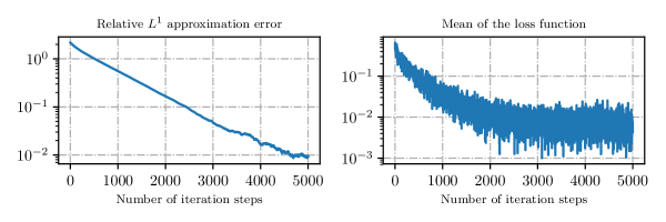
Figure 1: Plots of approximative calculations of the relative $L^{1}$-approximation error ${\mathbbm{E}}\big{[}\tfrac{|\Theta_{m}^{(1)}-0.30879|}{0.30879}\big{]}$ and of the mean of the loss function ${\mathbbm{E}}\big{[}|{\mathcal{Y}}^{m,\Theta_{m}}_{N}-g(\xi+W^{m}_{T})|^{2}\big{]}$ in the case of the $20$-dimensional Allen-Cahn equation (98) against $m\in\{0,1,\ldots,5000\}$.

4.2 Setting for the deep 2BSDE method with batch normalization and the Adam optimizer

Assume Framework 3.2, let $\varepsilon\in(0,\infty)$, $\beta_{1}=\tfrac{9}{10}$, $\beta_{2}=\tfrac{999}{1000}$, $(\gamma_{m})_{m\in{\mathbb{N}}_{0}}\subseteq(0,\infty)$, let $\operatorname{Pow}_{r}\colon{\mathbb{R}}^{\nu}\to{\mathbb{R}}^{\nu}$, $r\in(0,\infty)$, be the functions which satisfy for all $r\in(0,\infty)$, $x=(x_{1},\ldots,x_{\nu})\in{\mathbb{R}}^{\nu}$ that

$$\operatorname{Pow}_{r}(x)=(|x_{1}|^{r},\ldots,|x_{\nu}|^{r}),$$ (99)

let $u\colon[0,T]\times{\mathbb{R}}^{d}\to{\mathbb{R}}$ be an at most polynomially growing continuous function which satisfies for all $(t,x)\in[0,T)\times{\mathbb{R}}^{d}$ that $u(T,x)=g(x)$, $u|_{[0,T)\times{\mathbb{R}}^{d}}\in C^{1,2}([0,T)\times{\mathbb{R}}^{d},{\mathbb{R}})$, and

$$\tfrac{\partial u}{\partial t}(t,x)=f(t,x,u(t,x),(\nabla_{x}u)(t,x),(\operatorname{Hess}_{x}u)(t,x)),$$ (100)

assume for all $m\in{\mathbb{N}}_{0}$, $i\in\{0,1,\ldots,N\}$ that $J_{m}=64$, $t_{i}=\tfrac{iT}{N}$, and $\varrho=2\nu$, and assume for all $m\in{\mathbb{N}}_{0}$, $x=(x_{1},\ldots,x_{\nu}),~{}y=(y_{1},\ldots,y_{\nu})\in{\mathbb{R}}^{\nu}$, $\eta=(\eta_{1},\ldots,\eta_{\nu})\in{\mathbb{R}}^{\nu}$ that

$$\Psi_{m}(x,y,\eta)=(\beta_{1}x+(1-\beta_{1})\eta,\beta_{2}y+(1-\beta_{2})\operatorname{Pow}_{2}(\eta))$$ (101)

and

$$\psi_{m}(x,y)=\biggl{(}\Bigl{[}\sqrt{\tfrac{|y_{1}|}{1-\beta_{2}^{m}}}+\varepsilon\Bigr{]}^{-1}\frac{\gamma_{m}x_{1}}{1-\beta_{1}^{m}},\ldots,\Bigl{[}\sqrt{\tfrac{|y_{\nu}|}{1-\beta_{2}^{m}}}+\varepsilon\Bigr{]}^{-1}\frac{\gamma_{m}x_{\nu}}{1-\beta_{1}^{m}}\biggr{)}.$$ (102)

Remark 4.1.

Equations (101) and (102) describe the Adam optimizer; cf. Kingma & Ba [60] and lines 181–186 in Python code 3 in Subsection A.3 below. The default choice in TensorFlow for the real number $\varepsilon\in(0,\infty)$ in (102) is $\varepsilon=10^{-8}$ but according to the comments in the file adam.py in TensorFlow there are situations in which other choices may be more appropriate. In Subsection 4.5 we took $\varepsilon=1$ (in which case one has to add the argument epsilon=1.0 to tf.train.AdamOptimizer in lines 181–183 in Python code 3 in Subsection A.3 below) whereas we used the default value $\varepsilon=10^{-8}$ in Subsections 4.3, 4.4, and 4.6.

4.3 A $100$-dimensional Black-Scholes-Barenblatt equation

In this subsection we use the deep 2BSDE method in Framework 3.2 to approximatively calculate the solution of a $100$-dimensional Black-Scholes-Barenblatt equation (see Avellaneda, Levy, & Parás [2] and (105) below).

Assume the setting of Subsection 4.2, assume $d=100$, $T=1$, $N=20$, $\varepsilon=10^{-8}$, assume for all $\omega\in\Omega$ that $\xi(\omega)=(1,\nicefrac{{1}}{{2}},1,\nicefrac{{1}}{{2}},\ldots,1,\nicefrac{{1}}{{2}})\in{\mathbb{R}}^{d}$, let $r=\frac{5}{100}$, $\sigma_{\text{max}}=\frac{4}{10}$, $\sigma_{\text{min}}=\frac{1}{10}$, $\sigma_{c}=\frac{4}{10}$, let $\bar{\sigma}\colon{\mathbb{R}}\to{\mathbb{R}}$ be the function which satisfies for all $x\in{\mathbb{R}}$ that

$$\bar{\sigma}(x)=\begin{cases}\sigma_{\text{max}}&\colon x\geq 0\\ \sigma_{\text{min}}&\colon x<0\end{cases},$$ (103)

assume for all $s,t\in[0,T]$, $x=(x_{1},\ldots,x_{d}),w=(w_{1},\ldots,w_{d}),z=(z_{1},\ldots,z_{d})\in{\mathbb{R}}^{d}$, $y\in{\mathbb{R}}$, $S=(S_{ij})_{(i,j)\in\{1,\ldots,d\}^{2}}\in{\mathbb{R}}^{d\times d}$ that $\sigma(x)=\sigma_{c}\text{diag}(x_{1},\ldots,x_{d})$, $H(s,t,x,w)=x+\sigma(x)w$, $g(x)=\|x\|_{{\mathbb{R}}^{d}}^{2}$, and

$$f(t,x,y,z,S)=-\frac{1}{2}\sum_{i=1}^{d}|x_{i}|^{2}\,|\bar{\sigma}(S_{ii})|^{2}S_{ii}+r(y-\langle x,z\rangle_{{\mathbb{R}}^{d}}).$$ (104)

The solution $u\colon[0,T]\times{\mathbb{R}}^{d}\to{\mathbb{R}}$ of the PDE (100) then satisfies for all $(t,x)\in[0,T)\times{\mathbb{R}}^{d}$ that $u(T,x)=\|x\|_{{\mathbb{R}}^{d}}^{2}$ and

$$\tfrac{\partial u}{\partial t}(t,x)+\tfrac{1}{2}{\textstyle\sum\limits_{i=1}^{d}}|x_{i}|^{2}\big{|}\bar{\sigma}\big{(}\tfrac{\partial^{2}u}{\partial x_{i}^{2}}(t,x)\big{)}\big{|}^{2}\tfrac{\partial^{2}u}{\partial x_{i}^{2}}(t,x)=r\bigl{(}u(t,x)-\langle x,(\nabla_{x}u)(t,x)\rangle_{{\mathbb{R}}^{d}}\bigr{)}.$$ (105)

Number	Mean	Standard	Rel. $L^{1}$-	Standard	Mean	Standard	Runtime
of	of $\mathcal{U}^{\Theta_{m}}$	deviation	approx.	deviation	of the	deviation	in sec.
iteration		of $\mathcal{U}^{\Theta_{m}}$	error	of the	empirical	of the	for one
steps				relative	loss	empirical	realiz.
				approx.	function	loss	of $\mathcal{U}^{\Theta_{m}}$
				error		function
0	0.522	0.2292	0.9932	0.00297	5331.35	101.28	25
100	56.865	0.5843	0.2625	0.00758	441.04	90.92	191
200	74.921	0.2735	0.0283	0.00355	173.91	40.28	358
300	76.598	0.1636	0.0066	0.00212	96.56	17.61	526
400	77.156	0.1494	0.0014	0.00149	66.73	18.27	694

Table 2: Numerical simulations of the deep2BSDE method in Framework 3.2 in the case of the $100$-dimensional Black-Scholes-Barenblatt equation (105) (cf. Python code 3 in Subsection A.3 below). In the approximative calculations of the relative $L^{1}$-approximation errors the value $u(0,(1,\nicefrac{{1}}{{2}},1,\nicefrac{{1}}{{2}},\ldots,1,\nicefrac{{1}}{{2}}))$ has been replaced by the value 77.1049 which has been calculated by means of Lemma 4.2.

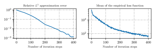
Figure 2: Plots of approximative calculations of the relative $L^{1}$-approximation error ${\mathbbm{E}}\big{[}\tfrac{|{\mathbbm{U}}^{\Theta_{m}}(\xi)-77.1049|}{77.1049}\big{]}$ and of the mean of the empirical loss function ${\mathbbm{E}}\big{[}\tfrac{1}{J_{m}}\sum_{j=1}^{J_{m}}|{\mathcal{Y}}^{m,\Theta_{m},j,\mathbb{S}_{m+1}}_{N}-g({\mathcal{X}}^{m,j}_{N})|^{2}\big{]}$ in the case of the $100$-dimensional Black-Scholes-Barenblatt equation (105) against $m\in\{0,1,\ldots,400\}$.

In Table 2 we use Python code 3 in Subsection A.3 below to approximatively calculate the mean ${\mathbbm{U}}^{\Theta_{m}}(\xi)$, the standard deviation of ${\mathbbm{U}}^{\Theta_{m}}(\xi)$, the relative $L^{1}$-approximation error associated to ${\mathbbm{U}}^{\Theta_{m}}(\xi)$, the uncorrected sample standard deviation of the relative approximation error associated to ${\mathbbm{U}}^{\Theta_{m}}(\xi)$, the mean of the empirical loss function associated to $\Theta_{m}$, the standard deviation of the empirical loss function associated to $\Theta_{m}$, and the average runtime in seconds needed for calculating one realization of ${\mathbbm{U}}^{\Theta_{m}}(\xi)$ against $m\in\{0,100,200,300,400\}$ based on $10$ realizations ($10$ independent runs of Python code 3 in Subsection A.3 below). In addition, Figure 2 depicts approximations of the relative $L^{1}$-approximation error and approximations of the mean of the empirical loss function associated to $\Theta_{m}$ against $m\in\{0,1,\ldots,400\}$ based on $10$ independent realizations ($10$ independent runs of Python code 3). In the approximative calculations of the relative $L^{1}$-approximation errors in Table 2 and Figure 2 the value $u(0,(1,\nicefrac{{1}}{{2}},1,\nicefrac{{1}}{{2}},\ldots,1,\nicefrac{{1}}{{2}}))$ of the solution $u$ of the PDE (105) has been replaced by the value $77.1049$ which, in turn, has been calculated by means of Lemma 4.2 below.

Lemma 4.2.

Let $c,\sigma_{\max},r,T\in(0,\infty)$, $\sigma_{\min}\in(0,\sigma_{\max})$, $d\in{\mathbb{N}}$, let $\bar{\sigma}\colon{\mathbb{R}}\to{\mathbb{R}}$ be the function which satisfies for all $x\in{\mathbb{R}}$ that

$$\bar{\sigma}(x)=\begin{cases}\sigma_{\max}&\colon x\geq 0\\ \sigma_{\min}&\colon x<0\end{cases},$$ (106)

and let $g\colon{\mathbb{R}}^{d}\to{\mathbb{R}}$ and $u\colon[0,T]\times{\mathbb{R}}^{d}\to{\mathbb{R}}$ be the functions which satisfy for all $t\in[0,T]$, $x=(x_{1},\dots,x_{d})\in{\mathbb{R}}^{d}$ that $g(x)=c\|x\|^{2}_{{\mathbb{R}}^{d}}=c\sum_{i=1}^{d}|x_{i}|^{2}$ and

$$u(t,x)=\exp\!\left([r+|\sigma_{\max}|^{2}](T-t)\right)g(x).$$ (107)

Then it holds for all $t\in[0,T]$, $x=(x_{1},\dots,x_{d})\in{\mathbb{R}}^{d}$ that $u\in C^{\infty}([0,T]\times{\mathbb{R}}^{d},{\mathbb{R}})$, $u(T,x)=g(x)$, and

$$\tfrac{\partial u}{\partial t}(t,x)+\tfrac{1}{2}{\textstyle\sum\limits_{i=1}^{d}}|x_{i}|^{2}\big{|}\bar{\sigma}\big{(}\tfrac{\partial^{2}u}{\partial x_{i}^{2}}(t,x)\big{)}\big{|}^{2}\tfrac{\partial^{2}u}{\partial x_{i}^{2}}(t,x)=r\big{(}u(t,x)-\langle x,(\nabla_{x}u)(t,x)\rangle_{{\mathbb{R}}^{d}}\big{)}.$$ (108)

Proof of Lemma 4.2.

Observe that the function $u$ is clearly infinitely often differentiable. Next note that (107) ensures that for all $t\in[0,T]$, $x=(x_{1},\dots,x_{d})\in{\mathbb{R}}^{d}$ it holds that

$$u(t,x)=\exp\!\left(-t[r+|\sigma_{\max}|^{2}]+T[r+|\sigma_{\max}|^{2}]\right)g(x).$$ (109)

Hence, we obtain that for all $t\in[0,T]$, $x=(x_{1},\dots,x_{d})\in{\mathbb{R}}^{d}$, $i\in\{1,2,\dots,d\}$ it holds that

$$\tfrac{\partial u}{\partial t}(t,x)=-[r+|\sigma_{\max}|^{2}]u(t,x),$$ (110)

$$\begin{split}\langle x,(\nabla_{x}u)(t,x)\rangle_{{\mathbb{R}}^{d}}&=\exp\!\left(-t[r+|\sigma_{\max}|^{2}]+T[r+|\sigma_{\max}|^{2}]\right)\left<x,(\nabla g)(x)\right>_{{\mathbb{R}}^{d}}\\ &=\exp\!\left(-t[r+|\sigma_{\max}|^{2}]+T[r+|\sigma_{\max}|^{2}]\right)\left<x,2cx\right>_{{\mathbb{R}}^{d}}\\ &=2c\exp\!\left(-t[r+|\sigma_{\max}|^{2}]+T[r+|\sigma_{\max}|^{2}]\right)\left\|x\right\|^{2}_{{\mathbb{R}}^{d}}=2u(t,x),\end{split}$$ (111)

and

$$\begin{split}\tfrac{\partial^{2}u}{\partial x_{i}^{2}}(t,x)&=2c\exp\!\left(-t[r+|\sigma_{\max}|^{2}]+T[r+|\sigma_{\max}|^{2}]\right)>0.\end{split}$$ (112)

Combining this with (106) demonstrates that for all $t\in[0,T]$, $x=(x_{1},\dots,x_{d})\in{\mathbb{R}}^{d}$, $i\in\{1,2,\dots,d\}$ it holds that

$$\begin{split}\bar{\sigma}\bigl{(}\tfrac{\partial^{2}u}{\partial x_{i}^{2}}(t,x)\bigr{)}=\sigma_{\max}.\end{split}$$ (113)

This and (110)–(112) ensure that for all $t\in[0,T]$, $x=(x_{1},\dots,x_{d})\in{\mathbb{R}}^{d}$ it holds that

$$\begin{split}&\tfrac{\partial u}{\partial t}(t,x)+\tfrac{1}{2}{\textstyle\sum\limits_{i=1}^{d}}|x_{i}|^{2}\big{|}\bar{\sigma}\big{(}\tfrac{\partial^{2}u}{\partial x_{i}^{2}}(t,x)\big{)}\big{|}^{2}\tfrac{\partial^{2}u}{\partial x_{i}^{2}}(t,x)-r\big{(}u(t,x)-\langle x,(\nabla_{x}u)(t,x)\rangle_{{\mathbb{R}}^{d}}\big{)}\\ &=-\left[r+|\sigma_{\max}|^{2}\right]u(t,x)+\tfrac{1}{2}{\textstyle\sum\limits_{i=1}^{d}}|x_{i}|^{2}\big{|}\bar{\sigma}\big{(}\tfrac{\partial^{2}u}{\partial x_{i}^{2}}(t,x)\big{)}\big{|}^{2}\tfrac{\partial^{2}u}{\partial x_{i}^{2}}(t,x)-r\big{(}u(t,x)-2u(t,x)\big{)}\\ &=-\left[r+|\sigma_{\max}|^{2}\right]u(t,x)+\tfrac{1}{2}{\textstyle\sum\limits_{i=1}^{d}}|x_{i}|^{2}|\sigma_{\max}|^{2}\tfrac{\partial^{2}u}{\partial x_{i}^{2}}(t,x)+ru(t,x)\\ &=\tfrac{1}{2}{\textstyle\sum\limits_{i=1}^{d}}|x_{i}|^{2}|\sigma_{\max}|^{2}\tfrac{\partial^{2}u}{\partial x_{i}^{2}}(t,x)-|\sigma_{\max}|^{2}u(t,x)=|\sigma_{\max}|^{2}\left[\tfrac{1}{2}{\textstyle\sum\limits_{i=1}^{d}}|x_{i}|^{2}\tfrac{\partial^{2}u}{\partial x_{1}^{2}}(t,x)-u(t,x)\right]\\ &=|\sigma_{\max}|^{2}\left[\tfrac{1}{2}\left\|x\right\|^{2}_{{\mathbb{R}}^{d}}\tfrac{\partial^{2}u}{\partial x_{1}^{2}}(t,x)-u(t,x)\right]\\ &=|\sigma_{\max}|^{2}\left[c\left\|x\right\|^{2}_{{\mathbb{R}}^{d}}\exp\!\left(-t[r+|\sigma_{\max}|^{2}]+T[r+|\sigma_{\max}|^{2}]\right)-u(t,x)\right]=0.\end{split}$$ (114)

The proof of Lemma 4.2 is thus completed. ∎

4.4 A $100$-dimensional Hamilton-Jacobi-Bellman equation

In this subsection we use the deep 2BSDE method in Framework 3.2 to approximatively calculate the solution of a $100$-dimensional Hamilton-Jacobi-Bellman equation with a nonlinearity that is quadratic in the gradient (see, e.g., [33, Section 4.3] and (116) below).

Assume the setting of Subsection 4.2, assume $d=100$, $T=1$, $N=20$, $\varepsilon=10^{-8}$, assume for all $\omega\in\Omega$ that $\xi(\omega)=(0,0,\ldots,0)\in{\mathbb{R}}^{d}$, and assume for all $m\in{\mathbb{N}}_{0}$, $s,t\in[0,T]$, $x,w,z\in{\mathbb{R}}^{d}$, $y\in{\mathbb{R}}$, $S\in{\mathbb{R}}^{d\times d}$ that $\sigma(x)=\sqrt{2}\,\operatorname{Id}_{{\mathbb{R}}^{d}}$, $H(s,t,x,w)=x+\sqrt{2}\,w$, $\gamma_{m}=\frac{1}{100}$, $g(x)=\ln(\frac{1}{2}[1+\|x\|_{{\mathbb{R}}^{d}}^{2}])$, and

$$f(t,x,y,z,S)=-\operatorname{Trace}(S)+\|z\|_{{\mathbb{R}}^{d}}^{2}.$$ (115)

The solution $u\colon[0,T]\times{\mathbb{R}}^{d}\to{\mathbb{R}}$ of the PDE (100) then satisfies for all $(t,x)\in[0,T)\times{\mathbb{R}}^{d}$ that

$$\tfrac{\partial u}{\partial t}(t,x)+(\Delta_{x}u)(t,x)=\|\nabla_{x}u(t,x)\|_{{\mathbb{R}}^{d}}^{2}.$$ (116)

In Table 3 we use an adapted version of Python code 3 in Subsection A.3 below to approximatively calculate the mean of ${\mathbbm{U}}^{\Theta_{m}}(\xi)$, the standard deviation of ${\mathbbm{U}}^{\Theta_{m}}(\xi)$, the relative $L^{1}$-approximation error associated to ${\mathbbm{U}}^{\Theta_{m}}(\xi)$, the uncorrected sample standard deviation of the relative approximation error associated to ${\mathbbm{U}}^{\Theta_{m}}(\xi)$, the mean of the empirical loss function associated to ${\mathbbm{U}}^{\Theta_{m}}(\xi)$, the standard deviation of the empirical loss function associated to ${\mathbbm{U}}^{\Theta_{m}}(\xi)$, and the average runtime in seconds needed for calculating one realization of ${\mathbbm{U}}^{\Theta_{m}}(\xi)$ against $m\in\{0,500,1000,1500,2000\}$ based on $10$ independent realizations ($10$ independent runs). In addition, Figure 3 depicts approximations of the mean of the relative $L^{1}$-approximation error and approximations of the mean of the empirical loss function associated to $\Theta_{m}$ against $m\in\{0,1,\ldots,2000\}$ based on $10$ independent realizations ($10$ independent runs). In the calculation of the relative $L^{1}$-approximation errors in Table 3 and Figure 3 the value $u(0,(0,0,\ldots,0))$ of the solution of the PDE (116) has been replaced by the value $4.5901$ which, in turn, was calculated by means of Lemma 4.2 in [33] (with $d=100$, $T=1$, $\alpha=1$, $\beta=-1$, $g={\mathbb{R}}^{d}\ni x\mapsto\ln(\tfrac{1}{2}[1+\|x\|_{{\mathbb{R}}^{d}}^{2}])\in{\mathbb{R}}$ in the notation of Lemma 4.2 in [33]) and the classical Monte Carlo method (cf. Matlab code 4 in Appendix A.4 below).

Number	Mean	Standard	Rel. $L^{1}$-	Standard	Mean	Standard	Runtime
of	of $\mathcal{U}^{\Theta_{m}}$	deviation	approx.	deviation	of the	deviation	in sec.
iteration		of $\mathcal{U}^{\Theta_{m}}$	error	of the	empirical	of the	for one
steps				relative	loss	empirical	realiz.
				approx.	function	loss	of $\mathcal{U}^{\Theta_{m}}$
				error		function
0	0.6438	0.2506	0.8597	0.05459	8.08967	1.65498	24
500	2.2008	0.1721	0.5205	0.03750	4.44386	0.51459	939
1000	3.6738	0.1119	0.1996	0.02437	1.46137	0.46636	1857
1500	4.4094	0.0395	0.0394	0.00860	0.26111	0.08805	2775
2000	4.5738	0.0073	0.0036	0.00159	0.05641	0.01412	3694

Table 3: Numerical simulations of the deep2BSDE method in Framework 3.2 in the case of the $100$-dimensional Hamilton-Jacobi-Bellman equation (116). In the approximative calculations of the relative $L^{1}$-approximation errors the value $u(0,(0,0,\ldots,0))$ has been replaced by the value 4.5901 which has been calculated by means of the classical Monte Carlo method (cf. Matlab code 4 in Appendix A.4 below).

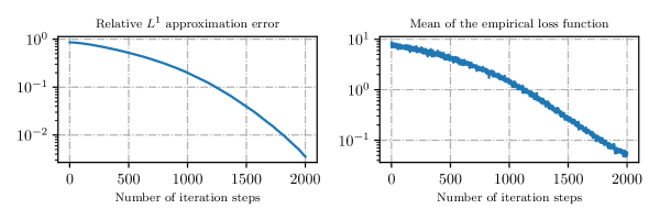
Figure 3: Plots of approximative calculations of the relative $L^{1}$-approximation error ${\mathbbm{E}}\big{[}\tfrac{|{\mathbbm{U}}^{\Theta_{m}}(\xi)-4.5901|}{4.5901}\big{]}$ and of the mean of the empirical loss function ${\mathbbm{E}}\big{[}\tfrac{1}{J_{m}}\sum_{j=1}^{J_{m}}|{\mathcal{Y}}^{m,\Theta_{m},j,\mathbb{S}_{m+1}}_{N}-g({\mathcal{X}}^{m,j}_{N})|^{2}\big{]}$ in the case of the $100$-dimensional Hamilton-Jacobi-Bellman equation (116) against $m\in\{0,1,\ldots,2000\}$.

4.5 A $50$-dimensional Allen-Cahn equation

In this subsection we use the deep 2BSDE method in Framework 3.2 to approximatively calculate the solution of a $50$-dimensional Allen-Cahn equation with a cubic nonlinearity (see (118) below).

Assume the setting of Subsection 4.2, assume $T=\tfrac{3}{10}$, $N=20$, $d=50$, $\varepsilon=1$, assume for all $\omega\in\Omega$ that $\xi(\omega)=(0,0,\ldots,0)\in{\mathbb{R}}^{50}$, and assume for all $m\in{\mathbb{N}}_{0}$, $s,t\in[0,T]$, $x,w,z\in{\mathbb{R}}^{d}$ $y\in{\mathbb{R}}$, $S\in{\mathbb{R}}^{d\times d}$ that $\sigma(x)=\sqrt{2}\operatorname{Id}_{{\mathbb{R}}^{d}}$, $H(s,t,x,w)=x+\sigma(x)w=x+\sqrt{2}w$, $g(x)=[2+\tfrac{2}{5}\|x\|_{{\mathbb{R}}^{d}}^{2}]^{-1}$, $f(t,x,y,z,S)=-\operatorname{Trace}(S)-y+y^{3}$, and

$$\gamma_{m}=\tfrac{1}{10}\cdot\left[\tfrac{9}{10}\right]^{\lfloor\frac{m}{1000}\rfloor}.$$ (117)

The solution $u$ to the PDE (100) then satisfies for all $(t,x)\in[0,T)\times{\mathbb{R}}^{d}$ that $u(T,x)=g(x)$ and

$$\tfrac{\partial u}{\partial t}(t,x)+\Delta u(t,x)+u(t,x)-\left[u(t,x)\right]^{3}=0.$$ (118)

In Table 4 we use an adapted version of Python code 3 in Subsection A.3 below to approximatively calculate the mean ${\mathbbm{U}}^{\Theta_{m}}(\xi)$, the standard deviation of ${\mathbbm{U}}^{\Theta_{m}}(\xi)$, the relative $L^{1}$-approximation error associated to ${\mathbbm{U}}^{\Theta_{m}}(\xi)$, the uncorrected sample standard deviation of the relative approximation error associated to ${\mathbbm{U}}^{\Theta_{m}}(\xi)$, the mean of the empirical loss function associated to ${\mathbbm{U}}^{\Theta_{m}}(\xi)$, the standard deviation of the empirical loss function associated to ${\mathbbm{U}}^{\Theta_{m}}(\xi)$, and the average runtime in seconds needed for calculating one realization of ${\mathbbm{U}}^{\Theta_{m}}(\xi)$ against $m\in\{0,500,1000,1500,2000\}$ based on $10$ independent realizations ($10$ independent runs). In addition, Figure 4 depicts approximations of the relative $L^{1}$-approximation error and approximations of the mean of the empirical loss function associated to $\Theta_{m}$ against $m\in\{0,1,\ldots,2000\}$ based on $10$ independent realizations ($10$ independent runs). In the approximate calculations of the relative $L^{1}$-approximation errors in Table 4 and Figure 4 the value $u(0,(0,0,\ldots,0))$ of the solution $u$ of the PDE (118) has been replaced by the value $0.09909$ which, in turn, has been calculated through the Branching diffusion method (cf. Matlab code 2 in Subsection A.2 below).

Number	Mean	Standard	Rel. $L^{1}$-	Standard	Mean	Standard	Runtime
of	of $\mathcal{U}^{\Theta_{m}}$	deviation	approx.	deviation	of the	deviation	in sec.
iteration		of $\mathcal{U}^{\Theta_{m}}$	error	of the	empirical	of the	for one
steps				relative	loss	empirical	realiz.
				approx.	function	loss	of $\mathcal{U}^{\Theta_{m}}$
				error		function
0	0.5198	0.19361	4.24561	1.95385	0.5830	0.4265	22
500	0.0943	0.00607	0.06257	0.04703	0.0354	0.0072	212
1000	0.0977	0.00174	0.01834	0.01299	0.0052	0.0010	404
1500	0.0988	0.00079	0.00617	0.00590	0.0008	0.0001	595
2000	0.0991	0.00046	0.00371	0.00274	0.0003	0.0001	787

Table 4: Numerical simulations of the deep2BSDE method in Framework 3.2 in the case of the $50$-dimensional Allen-Cahn equation (118). In the approximative calculations of the relative $L^{1}$-approximation errors the value $u(0,(0,0,\ldots,0))$ has been replaced by the value 0.09909 which has been calculated through the Branching diffusion method (cf. Matlab code 2 in Subsection A.2 below).

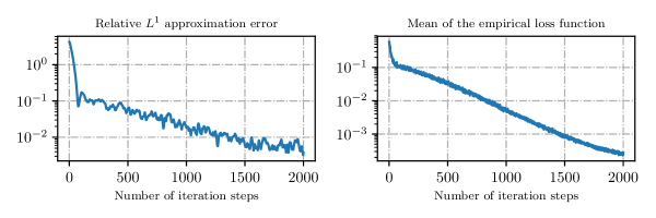
Figure 4: Plots of approximative calculations of the relative $L^{1}$-approximation error ${\mathbbm{E}}\big{[}\tfrac{|{\mathbbm{U}}^{\Theta_{m}}(\xi)-0.09909|}{0.09909}\big{]}$ and of the mean of the empirical loss function ${\mathbbm{E}}\big{[}\tfrac{1}{J_{m}}\sum_{j=1}^{J_{m}}|{\mathcal{Y}}^{m,\Theta_{m},j,\mathbb{S}_{m+1}}_{N}-g({\mathcal{X}}^{m,j}_{N})|^{2}\big{]}$ in the case of the $50$-dimensional Allen-Cahn equation (118) against $m\in\{0,1,\ldots,2000\}$.

4.6 $G$-Brownian motions in $1$ and $100$ space-dimensions

In this subsection we use the deep 2BSDE method in Framework 3.2 to approximatively calculate nonlinear expectations of a test function on a $100$-dimensional $G$-Brownian motion and of a test function on a $1$-dimensional $G$-Brownian motion. In the case of the $100$-dimensional $G$-Brownian motion we consider a specific test function such that the nonlinear expectation of this function on the $100$-dimensional $G$-Brownian motion admits an explicit analytic solution (see Lemma 4.3 below). In the case of the $1$-dimension $G$-Brownian motion we compare the numerical results of the deep 2BSDE method with numerical results obtained by a finite difference approximation method.

Assume the setting of Subsection 4.2, assume $T=1$, $N=20$, $\varepsilon=10^{-8}$, let $\sigma_{\text{max}}=1$, $\sigma_{\text{min}}=\tfrac{1}{\sqrt{2}}$, let $\bar{\sigma}\colon{\mathbb{R}}\to{\mathbb{R}}$ be the function which satisfies for all $x\in{\mathbb{R}}$ that

$$\bar{\sigma}(x)=\begin{cases}\sigma_{\text{max}}&\colon x\geq 0\\ \sigma_{\text{min}}&\colon x<0\end{cases},$$ (119)

assume for all $s,t\in[0,T]$, $x=(x_{1},\ldots,x_{d}),w=(w_{1},\ldots,w_{d}),z=(z_{1},\ldots,z_{d})\in{\mathbb{R}}^{d}$, $y\in{\mathbb{R}}$, $S=(S_{ij})_{(i,j)\in\{1,\ldots,d\}^{2}}\in{\mathbb{R}}^{d\times d}$ that $\sigma(x)=\operatorname{Id}_{{\mathbb{R}}^{d}}$, $H(s,t,x,w)=x+w$, $g(x)=\|x\|_{{\mathbb{R}}^{d}}^{2}$, and

$$f(t,x,y,z,S)=-\tfrac{1}{2}\sum_{i=1}^{d}\bigl{[}\bar{\sigma}(S_{ii})\bigr{]}^{2}S_{ii}.$$ (120)

The solution $u\colon[0,T]\times{\mathbb{R}}^{d}\to{\mathbb{R}}$ of the PDE (100) then satisfies for all $(t,x)\in[0,T)\times{\mathbb{R}}^{d}$ that $u(T,x)=g(x)$ and

$$\tfrac{\partial u}{\partial t}(t,x)+\tfrac{1}{2}{\textstyle\sum\limits_{i=1}^{d}}\big{|}\bar{\sigma}\big{(}\tfrac{\partial^{2}u}{\partial x_{i}^{2}}(t,x)\big{)}\big{|}^{2}\tfrac{\partial^{2}u}{\partial x_{i}^{2}}(t,x)=0.$$ (121)

Number	Mean	Standard	Rel. $L^{1}$-	Standard	Mean	Standard	Runtime
of	of $\mathcal{U}^{\Theta_{m}}$	deviation	approx.	deviation	of the	deviation	in sec.
iteration		of $\mathcal{U}^{\Theta_{m}}$	error	of the	empirical	of the	for one
steps				relative	loss	empirical	realiz.
				approx.	function	loss	of $\mathcal{U}^{\Theta_{m}}$
				error		function
0	0.46	0.35878	0.99716	0.00221	26940.83	676.70	24
500	164.64	1.55271	0.01337	0.00929	13905.69	2268.45	757
1000	162.79	0.35917	0.00242	0.00146	1636.15	458.57	1491
1500	162.54	0.14143	0.00074	0.00052	403.00	82.40	2221

Table 5: Numerical simulations of the deep2BSDE method in Framework 3.2 in the case of the $100$-dimensional $G$-Brownian motion (cf. (121) and (122)). In the approximative calculations of the relative $L^{1}$-approximation errors the value $u(0,(1,\nicefrac{{1}}{{2}},1,\nicefrac{{1}}{{2}},\ldots,1,\nicefrac{{1}}{{2}}))$ has been replaced by the value $162.5$ which has been calculated by means of Lemma 4.3.

Figure 5: Plots of approximative calculations of the relative $L^{1}$-approximation error ${\mathbbm{E}}\big{[}\tfrac{|{\mathbbm{U}}^{\Theta_{m}}(\xi)-162.5|}{162.5}\big{]}$ and of the mean of the empirical loss function ${\mathbbm{E}}\big{[}\tfrac{1}{J_{m}}\sum_{j=1}^{J_{m}}|{\mathcal{Y}}^{m,\Theta_{m},j,\mathbb{S}_{m+1}}_{N}-g({\mathcal{X}}^{m,j}_{N})|^{2}\big{]}$ in the case of the $100$-dimensional $G$-Brownian motion (cf. (121) and (122)) against $m\in\{0,1,\ldots,1500\}$.

In Table 5 we use an adapted version of Python code 3 to approximatively calculate the mean ${\mathbbm{U}}^{\Theta_{m}}(\xi)$, the standard deviation of ${\mathbbm{U}}^{\Theta_{m}}(\xi)$, the relative $L^{1}$-approximation error associated to ${\mathbbm{U}}^{\Theta_{m}}(\xi)$, the uncorrected sample standard deviation of the relative approximation error associated to ${\mathbbm{U}}^{\Theta_{m}}(\xi)$, the mean of the empirical loss function associated to ${\mathbbm{U}}^{\Theta_{m}}(\xi)$, the standard deviation of the empirical loss function associated to ${\mathbbm{U}}^{\Theta_{m}}(\xi)$, and the average runtime in seconds needed for calculating one realization of ${\mathbbm{U}}^{\Theta_{m}}(\xi)$ against $m\in\{0,500,1000,1500,2000\}$ based on $10$ realizations ($10$ independent runs) in the case where for all $x\in{\mathbb{R}}^{d}$, $m\in{\mathbb{N}}_{0}$, $\omega\in\Omega$ it holds that

$$\begin{split}d=100,\;\;g(x)=\|x\|_{{\mathbb{R}}^{d}}^{2},\;\;\gamma_{m}=\left[\tfrac{1}{2}\right]^{\lfloor\frac{m}{500}\rfloor},\;\;\text{and}\;\;\xi(\omega)=(1,\tfrac{1}{2},1,\tfrac{1}{2},\ldots,1,\tfrac{1}{2})\in{\mathbb{R}}^{d}.\end{split}$$ (122)

In addition, Figure 5 depicts approximations of the relative $L^{1}$-approximation error associated to ${\mathbbm{U}}^{\Theta_{m}}(\xi)$ and approximations of mean of the empirical loss function associated to $\Theta_{m}$ against $m\in\{0,1,\ldots,2000\}$ based on $10$ independent realizations ($10$ independent runs) in the case of (122). In the approximative calculations of the relative $L^{1}$-approximation errors in Table 5 and Figure 5 the value $u(0,(1,\nicefrac{{1}}{{2}},1,\nicefrac{{1}}{{2}},\ldots,1,\nicefrac{{1}}{{2}}))$ of the solution $u$ of the PDE (cf. (121) and (122)) has been replaced by the value $162.5$ which, in turn, has been calculated by means of Lemma 4.3 below (with $c=1$, $\sigma_{\max}=1$, $T=1$, $\sigma_{\min}=\nicefrac{{1}}{{\sqrt{2}}}$, $d=100$ in the notation of Lemma 4.3 below).

Lemma 4.3.

Let $c,\sigma_{\max},T\in(0,\infty)$, $\sigma_{\min}\in(0,\sigma_{\max})$, $d\in{\mathbb{N}}$, let $\bar{\sigma}\colon{\mathbb{R}}\to{\mathbb{R}}$ be the function which satisfies for all $x\in{\mathbb{R}}$ that

$$\bar{\sigma}(x)=\begin{cases}\sigma_{\max}&\colon x\geq 0\\ \sigma_{\min}&\colon x<0\end{cases},$$ (123)

and let $g\colon{\mathbb{R}}^{d}\to{\mathbb{R}}$ and $u\colon[0,T]\times{\mathbb{R}}^{d}\to{\mathbb{R}}$ be the functions which satisfy for all $t\in[0,T]$, $x=(x_{1},\ldots,x_{d})\in{\mathbb{R}}^{d}$ that $g(x)=c\|x\|^{2}_{{\mathbb{R}}^{d}}=c\sum_{i=1}^{d}|x_{i}|^{2}$ and

$$u(t,x)=g(x)+cd|\sigma_{\max}|^{2}(T-t).$$ (124)

Then it holds for all $t\in[0,T]$, $x=(x_{1},\ldots,x_{d})\in{\mathbb{R}}^{d}$ that $u\in C^{\infty}([0,T]\times{\mathbb{R}}^{d},{\mathbb{R}})$, $u(T,x)=g(x)$, and

$$\tfrac{\partial u}{\partial t}(t,x)+\tfrac{1}{2}{\textstyle\sum\limits_{i=1}^{d}}\big{|}\bar{\sigma}\big{(}\tfrac{\partial^{2}u}{\partial x_{i}^{2}}(t,x)\big{)}\big{|}^{2}\tfrac{\partial^{2}u}{\partial x_{i}^{2}}(t,x)=0.$$ (125)

Proof of Lemma 4.3.

Observe that the function $u$ is clearly infinitely often differentiable. Next note that (124) ensures that for all $t\in[0,T]$, $x=(x_{1},\ldots,x_{d})\in{\mathbb{R}}^{d}$, $i\in\{1,2,\ldots,d\}$ it holds that

$$\tfrac{\partial u}{\partial t}(t,x)=\tfrac{\partial}{\partial t}\bigl{[}g(x)+cd|\sigma_{\max}|^{2}(T-t)\bigr{]}=\tfrac{\partial}{\partial t}\bigl{[}cd|\sigma_{\max}|^{2}(T-t)\bigr{]}=-cd|\sigma_{\max}|^{2}$$ (126)

and

$$\tfrac{\partial^{2}u}{\partial x_{i}^{2}}(t,x)=\tfrac{\partial^{2}}{\partial x_{i}^{2}}\bigl{[}g(x)+cd|\sigma_{\max}|^{2}(T-t)\bigr{]}=\tfrac{\partial^{2}g}{\partial x_{i}^{2}}(x)=2c>0.$$ (127)

Combining this with (123) shows that for all $t\in[0,T]$, $x=(x_{1},\ldots,x_{d})\in{\mathbb{R}}^{d}$, $i\in\{1,2,\ldots,d\}$ it holds that

$$\bar{\sigma}\bigl{(}\tfrac{\partial^{2}u}{\partial x_{i}^{2}}(t,x)\bigr{)}=\bar{\sigma}(2c)=\sigma_{\max}.$$ (128)

This, (126), and (127) yield that for all $t\in[0,T]$, $x=(x_{1},\ldots,x_{d})\in{\mathbb{R}}^{d}$ it holds that

$$\begin{split}\tfrac{\partial u}{\partial t}(t,x)+\tfrac{1}{2}{\textstyle\sum\limits_{i=1}^{d}}\big{|}\bar{\sigma}\big{(}\tfrac{\partial^{2}u}{\partial x_{i}^{2}}(t,x)\big{)}\big{|}^{2}\tfrac{\partial^{2}u}{\partial x_{i}^{2}}(t,x)&=\tfrac{\partial u}{\partial t}(t,x)+\tfrac{1}{2}{\textstyle\sum\limits_{i=1}^{d}}|\sigma_{\max}|^{2}\tfrac{\partial^{2}u}{\partial x_{i}^{2}}(t,x)\\ &=\tfrac{\partial u}{\partial t}(t,x)+cd|\sigma_{\max}|^{2}=0.\end{split}$$ (129)

This completes the proof of Lemma 4.3. ∎

Number	Mean	Standard	Rel. $L^{1}$-	Standard	Mean	Standard	Runtime
of	of $\mathcal{U}^{\Theta_{m}}$	deviation	approx.	deviation	of the	deviation	in sec.
iteration		of $\mathcal{U}^{\Theta_{m}}$	error	of the	empirical	of the	for one
steps				relative	loss	empirical	realiz.
				approx.	function	loss	of $\mathcal{U}^{\Theta_{m}}$
				error		function
0	0.4069	0.28711	0.56094	0.29801	29.905	25.905	22
100	0.8621	0.07822	0.08078	0.05631	1.003	0.593	24
200	0.9097	0.01072	0.00999	0.00840	0.159	0.068	26
300	0.9046	0.00320	0.00281	0.00216	0.069	0.048	28
500	0.9017	0.00159	0.00331	0.00176	0.016	0.005	32

Table 6: Numerical simulations of the deep2BSDE method in Framework 3.2 in the case of the $1$-dimensional $G$-Brownian motion (cf. (121) and (130)). In the approximative calculations of the relative $L^{1}$-approximation error the value $u(0,-2)$ has been replaced by the value 0.90471 which has been calculated through finite differences approximations (cf. Matlab code 5 in Subsection A.5 below).

Figure 6: Plots of approximative calculations of the relative $L^{1}$-approximation error ${\mathbbm{E}}\big{[}\tfrac{|{\mathbbm{U}}^{\Theta_{m}}(\xi)-0.90471|}{0.90471}\big{]}$ and of the mean of the empirical loss function ${\mathbbm{E}}\big{[}\tfrac{1}{J_{m}}\sum_{j=1}^{J_{m}}|{\mathcal{Y}}^{m,\Theta_{m},j,\mathbb{S}_{m+1}}_{N}-g({\mathcal{X}}^{m,j}_{N})|^{2}\big{]}$ in the case of the $1$-dimensional $G$-Brownian motion (cf. (121) and (130)) against $m\in\{0,1,\ldots,500\}$.

In Table 6 we use an adapted version of Python code 3 in Subsection A.3 below to approximatively calculate the mean of ${\mathbbm{U}}^{\Theta_{m}}(\xi)$, the standard deviation of ${\mathbbm{U}}^{\Theta_{m}}(\xi)$, the relative $L^{1}$-approximation error associated to ${\mathbbm{U}}^{\Theta_{m}}(\xi)$, the uncorrected sample standard deviation of the relative approximation error associated to ${\mathbbm{U}}^{\Theta_{m}}(\xi)$, the mean of the empirical loss function associated to ${\mathbbm{U}}^{\Theta_{m}}(\xi)$, the standard deviation of the empirical loss function associated to ${\mathbbm{U}}^{\Theta_{m}}(\xi)$, and the average runtime in seconds needed for calculating one realization of ${\mathbbm{U}}^{\Theta_{m}}(\xi)$ against $m\in\{0,100,200,300,500\}$ based on $10$ realizations ($10$ independent runs) in the case where for all $x\in{\mathbb{R}}^{d}$, $m\in{\mathbb{N}}_{0}$, $\omega\in\Omega$ it holds that

$$\begin{split}d=1,\qquad g(x)=\tfrac{1}{1+\exp(-x^{2})},\qquad\gamma_{m}=\tfrac{1}{100},\qquad\text{and}\qquad\xi(\omega)=-2.\end{split}$$ (130)

In addition, Figure 6 depicts approximations of the relative $L^{1}$-approximation error associated to ${\mathbbm{U}}^{\Theta_{m}}(\xi)$ and approximations of the mean of empirical loss function associated to $\Theta_{m}$ for $m\in\{0,1,\ldots,500\}$ based on $10$ independent realizations ($10$ independent runs) in the case of (130). In the approximative calculations of the relative $L^{1}$-approximation errors in Table 5 and Figure 5 the value $u(0,-2)$ of the solution $u$ of the PDE (cf. (121) and (130)) has been replaced by the value $0.90471$ which, in turn, has been calculated by means of finite differences approximations (cf. Matlab code 5 in Subsection A.5 below).

Appendix A Source codes

A.1 A Python code for the deep 2BSDE method used in Subsection 4.1

The following Python code, Python code 1 below, is a simplified version of Python code 3 in Subsection A.3 below.

⬇

1#! /usr/bin/python3

2

3"""

4Plain deep2BSDE solver with hard-coded Allen-Cahn equation

5"""

6

7import tensorflow as tf

8import numpy as np

9import time, datetime

10

11tf.reset_default_graph()

12start_time = time.time()

13

14name = ’AllenCahn’

15

16# setting of the problem

17d = 20

18T = 0.3

19Xi = np.zeros([1,d])

20

21# setup of algorithm and implementation

22N = 20

23h = T/N

24sqrth = np.sqrt(h)

25n_maxstep = 10000

26batch_size = 1

27gamma = 0.001

28

29# neural net architectures

30n_neuronForGamma = [d, d, d, d**2]

31n_neuronForA = [d, d, d, d]

32

33# (adapted) rhs of the pde

34def f0(t,X,Y,Z,Gamma):

35 return -Y+tf.pow(Y, 3)

36

37# terminal condition

38def g(X):

39 return 1/(1 + 0.2*tf.reduce_sum(tf.square(X),

40 1, keep_dims=True))*0.5

41

42# helper functions for constructing the neural net(s)

43def _one_time_net(x, name, isgamma = False):

44 with tf.variable_scope(name):

45 layer1 = _one_layer(x, (1-isgamma)*n_neuronForA[1] \

46 +isgamma*n_neuronForGamma[1], name = ’layer1’)

47 layer2 = _one_layer(layer1, (1-isgamma)*n_neuronForA[2] \

48 +isgamma*n_neuronForGamma[2], name = ’layer2’)

49 z = _one_layer(layer2, (1-isgamma)*n_neuronForA[3] \

50 +isgamma*n_neuronForGamma[3], activation_fn=None,

51 name = ’final’)

52 return z

53

54def _one_layer(input_, output_size, activation_fn=tf.nn.relu,

55 stddev=5.0, name=’linear’):

56 with tf.variable_scope(name):

57 shape = input_.get_shape().as_list()

58 w = tf.get_variable(’Matrix’, [shape[1], output_size],

59 tf.float64,

60 tf.random_normal_initializer(

61 stddev=stddev/np.sqrt(shape[1]+output_size)))

62 b = tf.get_variable(’Bias’, [1,output_size], tf.float64,

63 tf.constant_initializer(0.0))

64 hidden = tf.matmul(input_, w) + b

65 if activation_fn:

66 return activation_fn(hidden)

67 else:

68 return hidden

69

70with tf.Session() as sess:

71 # background dynamics

72 dW = tf.random_normal(shape=[batch_size, d], stddev = sqrth,

73 dtype=tf.float64)

74

75 # initial values of the stochastic processes

76 X = tf.Variable(np.ones([batch_size, d]) * Xi,

77 dtype = tf.float64,

78 name=’X’,

79 trainable=False)

80 Y0 = tf.Variable(tf.random_uniform([1],

81 minval = -1, maxval = 1,

82 dtype=tf.float64),

83 name=’Y0’)

84 Z0 = tf.Variable(tf.random_uniform([1,d],

85 minval = -.1, maxval = .1,

86 dtype=tf.float64),

87 name=’Z0’)

88 Gamma0 = tf.Variable(tf.random_uniform([d, d],

89 minval = -.1, maxval = .1,

90 dtype=tf.float64),

91 name=’Gamma0’)

92 A0 = tf.Variable(tf.random_uniform([1,d],

93 minval = -.1, maxval = .1,

94 dtype=tf.float64),

95 name=’A0’)

96 allones = tf.ones(shape=[batch_size, 1],

97 dtype=tf.float64,

98 name=’MatrixOfOnes’)

99 Y = allones * Y0

100 Z = tf.matmul(allones,Z0)

101 Gamma = tf.multiply(tf.ones([batch_size, d, d],

102 dtype = tf.float64), Gamma0)

103 A = tf.matmul(allones,A0)

104

105 # forward discretization

106 with tf.variable_scope(’forward’):

107 for i in range(N-1):

108 Y = Y + f0(i*h,X,Y,Z,Gamma)*h \

109 + tf.reduce_sum(dW*Z, 1, keep_dims=True)

110 Z = Z + A * h \

111 + tf.squeeze(tf.matmul(Gamma,

112 tf.expand_dims(dW, -1)))

113 Gamma = tf.reshape(_one_time_net(X, name=str(i)+’Gamma’,

114 isgamma=True)/d**2,

115 [batch_size, d, d])

116 if i!=N-1:

117 A = _one_time_net(X, name=str(i)+’A’)/d

118 X = X + dW

119 dW = tf.random_normal(shape=[batch_size, d],

120 stddev = sqrth, dtype=tf.float64)

121

122 Y = Y + f0( (N-1)*h , X,Y,Z,Gamma)*h \

123 + tf.reduce_sum(dW*Z, 1, keep_dims=True)

124 X = X + dW

125 loss_function = tf.reduce_mean(tf.square(Y-g(X)))

126

127 # specifying the optimizer

128 global_step = tf.get_variable(’global_step’, [],

129 initializer=tf.constant_initializer(0),

130 trainable=False, dtype=tf.int32)

131

132 learning_rate = tf.train.exponential_decay(gamma, global_step,

133 decay_steps = 10000, decay_rate = 0.0, staircase = True)

134

135 trainable_variables = tf.trainable_variables()

136 grads = tf.gradients(loss_function, trainable_variables)

137 optimizer = tf.train.GradientDescentOptimizer(

138 learning_rate=learning_rate)

139 apply_op = optimizer.apply_gradients(

140 zip(grads, trainable_variables),

141 global_step=global_step, name=’train_step’)

142

143 with tf.control_dependencies([apply_op]):

144 train_op_2 = tf.identity(loss_function, name=’train_op2’)

145

146 # to save history

147 learning_rates = []

148 y0_values = []

149 losses = []

150 running_time = []

151 steps = []

152 sess.run(tf.global_variables_initializer())

153

154 try:

155 # the actual training loop

156 for _ in range(n_maxstep + 1):

157 y0_value, step = sess.run([Y0, global_step])

158 currentLoss, currentLearningRate = sess.run(

159 [train_op_2, learning_rate])

160

161 learning_rates.append(currentLearningRate)

162 losses.append(currentLoss)

163 y0_values.append(y0_value)

164 running_time.append(time.time()-start_time)

165 steps.append(step)

166

167 if step % 100 == 0:

168 print("step: ", step,

169 " loss: ", currentLoss,

170 " Y0: " , y0_value,

171 " learning rate: ", currentLearningRate)

172

173 end_time = time.time()

174 print("running time: ", end_time-start_time)

175

176 except KeyboardInterrupt:

177 print("\nmanually disengaged")

178

179# writing results to a csv file

180output = np.zeros((len(y0_values),5))

181output[:,0] = steps

182output[:,1] = losses

183output[:,2] = y0_values

184output[:,3] = learning_rates

185output[:,4] = running_time

186

187np.savetxt("./" + str(name) + "_d" + str(d) + "_" + \

188 datetime.datetime.now().strftime(’%Y-%m-%d-%H:%M:%S’)+ ".csv",

189 output,

190 delimiter = ",",

191 header = "step, loss function, Y0, learning rate, running time",

192 )

Python code 1: A Python code for the deep 2BSDE method used in Subsection 4.1. This Python code uses the plain stochastic gradient descent method and does not use batch normalization.

A.2 A Matlab code for the Branching diffusion method used in Subsection 4.1

The following Matlab code is a slightly modified version of the Matlab code in E, Han, & Jentzen [33, Subsection 6.2].

⬇

1function Branching()

2 rng(’default’);

3

4% Parameter

5 T = 0.3;

6 M = 10^7;

7 t0 = 0;

8

9 d = 20; m = d;

10 beta = 1;

11 mu = zeros(d,1);

12 sigma = eye(d);

13 a = [0 2 0 -1]’;

14 p = [0 0.5 0 0.5]’;

15 psi = @(x) 1./(1+0.2*norm(x)^2)*1/2;

16 x0 = 0;

17

18% Branching PDE Solver

19 tic;

20 [result,SD] = ...

21 MCBranchingEvaluation(...

22 mu, sigma, beta, p, a, t0, x0, T, psi, M);

23 runtime = toc;

24 disp([’BranchingP solver: u(0,x0) = ’ num2str(result) ’;’]);

25 disp([’Runtime = ’ num2str(runtime) ’;’]);

26end

27

28 function [result,SD] = ...

29 MCBranchingEvaluation(...

30 mu, sigma, beta, p, a, t0, x0, T, psi, M)

31 result = 0;

32 SD = 0;

33 for m=1:M

34 Evl = BranchingEvaluation(...

35 mu, sigma, beta, p, a, t0, x0, T, psi);

36 result = result + Evl;

37 SD = SD + Evl^2;

38 end

39 SD = sqrt( (SD - result^2/M)/M );

40 result = result/M;

41 end

42

43 function Evl = ...

44 BranchingEvaluation(...

45 mu, sigma, beta, p, a, t0, x0, T, psi)

46 BP = BranchingProcess(mu, sigma, beta, p, t0, x0, T);

47 Evl = 1;

48 for k=1:size(BP{1},2)

49 Evl = Evl * psi( BP{1}(:,k) );

50 end

51 if norm(a-p) > 0

52 for k=1:length(a)

53 if p(k) > 0

54 Evl = Evl * ( a(k)/p(k) )^( BP{2}(k) );

55 elseif a(k) ~= 0

56 error(’a(k) zero but p(k) non-zero’);

57 end

58 end

59 end

60 end

61

62 function BP = ...

63 BranchingProcess(mu, sigma, beta, p, t0, x0, T)

64 BP = cell(2,1);

65 BP{2} = p*0;

66 tau = exprnd(1/beta);

67 new_t0 = min( tau + t0, T );

68 delta_t = new_t0 - t0;

69 m = size(sigma,2);

70 new_x0 = x0 + mu*delta_t + sigma*sqrt(delta_t)*randn(m,1);

71 if tau >= T - t0

72 BP{1} = new_x0;

73 else

74 [tmp,which_nonlinearity] = max(mnrnd(1,p));

75 BP{2}(which_nonlinearity) = BP{2}(which_nonlinearity) + 1;

76 for k=1:which_nonlinearity-1

77 tmp = BranchingProcess(...

78 mu, sigma, beta, p, new_t0, new_x0, T);

79 BP{1} = [ BP{1} tmp{1} ];

80 BP{2} = BP{2} + tmp{2};

81 end

82 end

83 end

Matlab code 2: A Matlab code for the Branching diffusion method used in Subsection 4.5.

A.3 A Python code for the deep 2BSDE method used in Subsection 4.3

The following Python code is based on the Python code in E, Han, & Jentzen [33, Subsection 6.1].

⬇

1#!/usr/bin/python3

2# -*- coding: utf-8 -*-

3

4"""

5Deep2BSDE solver with hard-coded Black-Scholes-Barenblatt equation.

6"""

7

8import time, datetime

9import tensorflow as tf

10import numpy as np

11from tensorflow.python.training import moving_averages

12

13start_time = time.time()

14tf.reset_default_graph()

15

16name = ’BSB’

17d = 100

18batch_size = 64

19T = 1.0

20N = 20

21h = T/N

22sqrth = np.sqrt(h)

23n_maxstep = 500

24n_displaystep = 100

25n_neuronForA = [d,d,d,d]

26n_neuronForGamma = [d,d,d,d**2]

27Xinit = np.array([1.0,0.5]*50)

28mu = 0

29sigma = 0.4

30sigma_min = 0.1

31sigma_max = 0.4

32r = 0.05

33

34_extra_train_ops = []

35

36def sigma_value(W):

37 return sigma_max * \

38 tf.cast(tf.greater_equal(W, tf.cast(0,tf.float64)),

39 tf.float64) + \

40 sigma_min * tf.cast(tf.greater(tf.cast(0,tf.float64), W),

41 tf.float64)

42

43def f_tf(t, X, Y, Z, Gamma):

44 return -0.5*tf.expand_dims(tf.trace(

45 tf.square(tf.expand_dims(X,-1)) * \

46 (tf.square(sigma_value(Gamma))-sigma**2) * Gamma),-1) + \

47 r * (Y - tf.reduce_sum(X*Z, 1, keep_dims = True))

48

49def g_tf(X):

50 return tf.reduce_sum(tf.square(X),1, keep_dims = True)

51

52def sigma_function(X):

53 return sigma * tf.matrix_diag(X)

54

55def mu_function(X):

56 return mu * X

57

58def _one_time_net(x, name, isgamma = False):

59 with tf.variable_scope(name):

60 x_norm = _batch_norm(x, name=’layer0_normalization’)

61 layer1 = _one_layer(x_norm, (1-isgamma)*n_neuronForA[1] \

62 +isgamma*n_neuronForGamma[1], name = ’layer1’)

63 layer2 = _one_layer(layer1, (1-isgamma)*n_neuronForA[2] \

64 +isgamma*n_neuronForGamma[2], name = ’layer2’)

65 z = _one_layer(layer2, (1-isgamma)*n_neuronForA[3] \

66 +isgamma*n_neuronForGamma[3], activation_fn=None,

67 name = ’final’)

68 return z

69

70def _one_layer(input_, output_size, activation_fn=tf.nn.relu,

71 stddev=5.0, name=’linear’):

72 with tf.variable_scope(name):

73 shape = input_.get_shape().as_list()

74 w = tf.get_variable(’Matrix’, [shape[1], output_size],

75 tf.float64,

76 tf.random_normal_initializer(

77 stddev=stddev/np.sqrt(shape[1]+output_size)))

78 hidden = tf.matmul(input_, w)

79 hidden_bn = _batch_norm(hidden, name=’normalization’)

80 if activation_fn:

81 return activation_fn(hidden_bn)

82 else:

83 return hidden_bn

84

85def _batch_norm(x, name):

86 """Batch normalization"""

87 with tf.variable_scope(name):

88 params_shape = [x.get_shape()[-1]]

89 beta = tf.get_variable(’beta’, params_shape, tf.float64,

90 initializer=tf.random_normal_initializer(

91 0.0, stddev=0.1, dtype=tf.float64))

92 gamma = tf.get_variable(’gamma’, params_shape, tf.float64,

93 initializer=tf.random_uniform_initializer(

94 0.1, 0.5, dtype=tf.float64))

95 moving_mean = tf.get_variable(’moving_mean’,

96 params_shape, tf.float64,

97 initializer=tf.constant_initializer(0.0, tf.float64),

98 trainable=False)

99 moving_variance = tf.get_variable(’moving_variance’,

100 params_shape, tf.float64,

101 initializer=tf.constant_initializer(1.0, tf.float64),

102 trainable=False)

103 mean, variance = tf.nn.moments(x, [0], name=’moments’)

104 _extra_train_ops.append(

105 moving_averages.assign_moving_average(

106 moving_mean, mean, 0.99))

107 _extra_train_ops.append(

108 moving_averages.assign_moving_average(

109 moving_variance, variance, 0.99))

110 y = tf.nn.batch_normalization(

111 x, mean, variance, beta, gamma, 1e-6)

112 y.set_shape(x.get_shape())

113 return y

114

115with tf.Session() as sess:

116

117 dW = tf.random_normal(shape=[batch_size, d],

118 stddev = 1, dtype=tf.float64)

119 X = tf.Variable(np.ones([batch_size, d]) * Xinit,

120 dtype=tf.float64,

121 trainable=False)

122 Y0 = tf.Variable(tf.random_uniform(

123 [1],

124 minval=0, maxval=1, dtype=tf.float64),

125 name=’Y0’);

126 Z0 = tf.Variable(tf.random_uniform(

127 [1, d],

128 minval=-.1, maxval=.1,

129 dtype=tf.float64),

130 name=’Z0’)

131 Gamma0 = tf.Variable(tf.random_uniform(

132 [d, d],

133 minval=-1, maxval=1,

134 dtype=tf.float64), name=’Gamma0’)

135 A0 = tf.Variable(tf.random_uniform(

136 [1, d], minval=-.1, maxval=.1,

137 dtype=tf.float64), name=’A0’)

138 allones = tf.ones(shape=[batch_size, 1], dtype=tf.float64,

139 name=’MatrixOfOnes’)

140 Y = allones * Y0

141 Z = tf.matmul(allones, Z0)

142 A = tf.matmul(allones, A0)

143 Gamma = tf.multiply(tf.ones(shape=[batch_size, d, d],

144 dtype=tf.float64), Gamma0)

145 with tf.variable_scope(’forward’):

146 for t in range(0, N-1):

147 # Y update inside the loop

148 dX = mu * X * h + sqrth * sigma * X * dW

149 Y = Y + f_tf(t * h, X, Y, Z, Gamma)*h \

150 + tf.reduce_sum(Z*dX, 1, keep_dims = True)

151 X = X + dX

152 # Z update inside the loop

153 Z = Z + A * h \

154 + tf.squeeze(tf.matmul(Gamma,

155 tf.expand_dims(dX, -1),

156 transpose_b=False))

157 A = _one_time_net(X, str(t+1)+"A" )/d

158 Gamma = _one_time_net(X, str(t+1)+"Gamma",

159 isgamma = True)/d**2

160 Gamma = tf.reshape(Gamma, [batch_size, d, d])

161 dW = tf.random_normal(shape=[batch_size, d],

162 stddev = 1, dtype=tf.float64)

163 # Y update outside of the loop - terminal time step

164 dX = mu * X * h + sqrth * sigma * X * dW

165 Y = Y + f_tf((N-1) * h, X, Y, Z, Gamma)*h \

166 + tf.reduce_sum(Z * dX, 1, keep_dims=True)

167 X = X + dX

168 loss = tf.reduce_mean(tf.square(Y-g_tf(X)))

169

170 # training operations

171 global_step = tf.get_variable(’global_step’, [],

172 initializer=tf.constant_initializer(0),

173 trainable=False, dtype=tf.int32)

174

175 learning_rate = tf.train.exponential_decay(1.0, global_step,

176 decay_steps = 200,

177 decay_rate = 0.5,

178 staircase=True)

179

180 trainable_variables = tf.trainable_variables()

181 grads = tf.gradients(loss, trainable_variables)

182 optimizer = tf.train.AdamOptimizer(

183 learning_rate=learning_rate

184 )

185 apply_op = optimizer.apply_gradients(

186 zip(grads, trainable_variables),

187 global_step=global_step, name=’train_step’)

188 train_ops = [apply_op] + _extra_train_ops

189 train_op = tf.group(*train_ops)

190

191 with tf.control_dependencies([train_op]):

192 train_op_2 = tf.identity(loss, name=’train_op2’)

193

194 # to save history

195 learning_rates = []

196 y0_values = []

197 losses = []

198 running_time = []

199 steps = []

200 sess.run(tf.global_variables_initializer())

201

202 try:

203

204 for _ in range(n_maxstep+1):

205 step, y0_value = sess.run([global_step, Y0])

206 currentLoss, currentLearningRate = sess.run(

207 [train_op_2, learning_rate])

208

209 steps.append(step)

210 losses.append(currentLoss)

211 y0_values.append(y0_value)

212 learning_rates.append(currentLearningRate)

213 running_time.append(time.time()-start_time)

214

215 if step % n_displaystep == 0:

216 print("step: ", step,

217 " loss: ", currentLoss,

218 " Y0: " , y0_value,

219 " learning rate: ", currentLearningRate)

220

221 end_time = time.time()

222 print("running time: ", end_time-start_time)

223

224 except KeyboardInterrupt:

225 print("manually disengaged")

226

227# writing results to a csv file

228output = np.zeros((len(y0_values),5))

229output[:,0] = steps

230output[:,1] = losses

231output[:,2] = y0_values

232output[:,3] = learning_rates

233output[:,4] = running_time

234np.savetxt("./" + str(name) + "_d" + str(d) + "_" + \

235 datetime.datetime.now().strftime(’%Y-%m-%d-%H:%M:%S’) + ".csv",

236 output,

237 delimiter = ",",

238 header = "step, loss function, Y0, learning rate, running time"

239 )

Python code 3: A Python code for the deep 2BSDE method used in Subsection 4.3.

A.4 A Matlab code for the classical Monte Carlo method used in Subsection 4.4

The following Matlab code is a slightly modified version of the Matlab code in E, Han, & Jentzen [33, Subsection 6.3].

⬇

1rng(’default’);

2M = 10^7;

3d = 100;

4MC = 0;

5for m=1:M

6 dW = randn(1,d);

7 MC = MC + 2/(1+norm(sqrt(2)*dW)^2);

8end

9MC = -log(MC/M);

Matlab code 4: A Matlab code for the classical Monte Carlo method used in Subsection 4.4.

A.5 A Matlab code for the finite differences method used in Subsection 4.6

The following Matlab code is inspired by the Matlab code in E et al. [35, MATLAB code 7 in Section 3].

⬇

1function GBrownianMotion()

2 disp(num2str(finiteDiff_GBrownianMotion(0,-2,1000)))

3end

4

5function y = finiteDiff_GBrownianMotion(t0,x0,N)

6 sigma_max = 1.0;

7 sigma_min = 0.5;

8 T = 1.0;

9 sigma = 1;

10 f = @(t,x,y,z,gamma) 0.5 * ((gamma>0).*sigma_max ...

11 + (gamma<=0).*sigma_min).* gamma;

12

13 g = @(x) 1./(1+exp(-x.^2));

14 h=(T-t0)./N;

15 t=t0:h:T;

16 d1 = 0.05;

17 d2=sigma*d1;

18 x=x0+d1*(-N:1:N);

19 M=(1/(h)*[[1, zeros(1,2.*N-2)];

20 full(gallery(’tridiag’,...

21 ones(2.*N-2,1),-2*ones(2.*N-1,1),ones(2.*N-2,1)));

22 [zeros(1,2*N-2),1]]);

23 L=1/(2*d1)*([[-1, zeros(1,2.*N-2)];

24 full(gallery(’tridiag’,...

25 ones(2.*N-2,1),zeros(2.*N-1,1),-ones(2.*N-2,1)));

26 [zeros(1,2*N-2),1]]);

27 y=g(x);

28 for i=N:-1:1

29 x=x(1:(2*i-1))+d2;

30 tmp = y(2:(2*i));

31 z=y*L(1:(2*i+1),1:(2*i-1));

32 gamma=y*M(1:(2*i+1),1:(2*i-1));

33 y=tmp+h*f(t(i),x,tmp,z,gamma);

34 end

35end

Matlab code 5: A Matlab code for the finite differences method used in Subsection 4.6.

Acknowledgements

Sebastian Becker and Jiequn Han are gratefully acknowledged for their helpful and inspiring comments regarding the implementation of the deep 2BSDE method.

References

• [1] Amadori, A. L. Nonlinear integro-differential evolution problems arising in option pricing: a viscosity solutions approach. Differential Integral Equations 16, 7 (2003), 787–811.
• [2] Avellaneda, M., ∗, A. L., and Parás, A. Pricing and hedging derivative securities in markets with uncertain volatilities. Appl. Math. Finance 2, 2 (1995), 73–88.
• [3] Bally, V., and Pagès, G. A quantization algorithm for solving multi-dimensional discrete-time optimal stopping problems. Bernoulli 9, 6 (2003), 1003–1049.
• [4] Bayraktar, E., Milevsky, M. A., Promislow, S. D., and Young, V. R. Valuation of mortality risk via the instantaneous Sharpe ratio: applications to life annuities. J. Econom. Dynam. Control 33, 3 (2009), 676–691.
• [5] Bayraktar, E., and Young, V. Pricing options in incomplete equity markets via the instantaneous sharpe ratio. Ann. Finance 4, 4 (2008), 399–429.
• [6] Bender, C., and Denk, R. A forward scheme for backward SDEs. Stochastic Process. Appl. 117, 12 (2007), 1793–1812.
• [7] Bender, C., Schweizer, N., and Zhuo, J. A primal-–dual algorithm for BSDEs. Math. Finance 27, 3 (2017), 866–901.
• [8] Bengio, Y. Learning deep architectures for AI. Foundations and Trends in Machine Learning 2, 1 (2009), 1–127.
• [9] Bergman, Y. Z. Option pricing with differential interest rates. The Review of Financial Studies 8, 2 (1995), 475–500.
• [10] Bismut, J.-M. Conjugate convex functions in optimal stochastic control. J. Math. Anal. Appl. 44 (1973), 384–404.
• [11] Bouchard, B. Lecture notes on BSDEs: Main existence and stability results. PhD thesis, CEREMADE-Centre de Recherches en MAthématiques de la DEcision, 2015.
• [12] Bouchard, B., Elie, R., and Touzi, N. Discrete-time approximation of BSDEs and probabilistic schemes for fully nonlinear PDEs. In Advanced financial modelling, vol. 8 of Radon Ser. Comput. Appl. Math. Walter de Gruyter, Berlin, 2009, pp. 91–124.
• [13] Bouchard, B., and Touzi, N. Discrete-time approximation and Monte-Carlo simulation of backward stochastic differential equations. Stochastic Process. Appl. 111, 2 (2004), 175–206.
• [14] Briand, P., and Labart, C. Simulation of BSDEs by Wiener chaos expansion. Ann. Appl. Probab. 24, 3 (2014), 1129–1171.
• [15] Cai, Z. Approximating quantum many-body wave-functions using artificial neural networks. arXiv:1704.05148 (2017), 8 pages.
• [16] Carleo, G., and Troyer, M. Solving the quantum many-body problem with artificial neural networks. Science 355, 6325 (2017), 602–606.
• [17] Chang, D., Liu, H., and Xiong, J. A branching particle system approximation for a class of FBSDEs. Probab. Uncertain. Quant. Risk 1 (2016), Paper No. 9, 34.
• [18] Chassagneux, J.-F. Linear multistep schemes for BSDEs. SIAM J. Numer. Anal. 52, 6 (2014), 2815–2836.
• [19] Chassagneux, J.-F., and Crisan, D. Runge-Kutta schemes for backward stochastic differential equations. Ann. Appl. Probab. 24, 2 (2014), 679–720.
• [20] Chassagneux, J.-F., and Richou, A. Numerical stability analysis of the Euler scheme for BSDEs. SIAM J. Numer. Anal. 53, 2 (2015), 1172–1193.
• [21] Chassagneux, J.-F., and Richou, A. Numerical simulation of quadratic BSDEs. Ann. Appl. Probab. 26, 1 (2016), 262–304.
• [22] Cheridito, P., Soner, H. M., Touzi, N., and Victoir, N. Second-order backward stochastic differential equations and fully nonlinear parabolic PDEs. Comm. Pure Appl. Math. 60, 7 (2007), 1081–1110.
• [23] Chiaramonte, M., and Kiener, M. Solving differential equations using neural networks. Machine Learning Project, 5 pages.
• [24] Crépey, S., Gerboud, R., Grbac, Z., and Ngor, N. Counterparty risk and funding: the four wings of the TVA. Int. J. Theor. Appl. Finance 16, 2 (2013), 1350006, 31.
• [25] Crisan, D., and Manolarakis, K. Probabilistic methods for semilinear partial differential equations. Applications to finance. M2AN Math. Model. Numer. Anal. 44, 5 (2010), 1107–1133.
• [26] Crisan, D., and Manolarakis, K. Solving backward stochastic differential equations using the cubature method: application to nonlinear pricing. SIAM J. Financial Math. 3, 1 (2012), 534–571.
• [27] Crisan, D., and Manolarakis, K. Second order discretization of backward SDEs and simulation with the cubature method. Ann. Appl. Probab. 24, 2 (2014), 652–678.
• [28] Crisan, D., Manolarakis, K., and Touzi, N. On the Monte Carlo simulation of BSDEs: an improvement on the Malliavin weights. Stochastic Process. Appl. 120, 7 (2010), 1133–1158.
• [29] Darbon, J., and Osher, S. Algorithms for overcoming the curse of dimensionality for certain Hamilton-Jacobi equations arising in control theory and elsewhere. Res. Math. Sci. 3 (2016), Paper No. 19, 26.
• [30] Dehghan, M., Nourian, M., and Menhaj, M. B. Numerical solution of Helmholtz equation by the modified Hopfield finite difference techniques. Numer. Methods Partial Differential Equations 25, 3 (2009), 637–656.
• [31] Delarue, F., and Menozzi, S. A forward-backward stochastic algorithm for quasi-linear PDEs. Ann. Appl. Probab. 16, 1 (2006), 140–184.
• [32] Douglas, Jr., J., Ma, J., and Protter, P. Numerical methods for forward-backward stochastic differential equations. Ann. Appl. Probab. 6, 3 (1996), 940–968.
• [33] E, W., Han, J., and Jentzen, A. Deep learning-based numerical methods for high-dimensional parabolic partial differential equations and backward stochastic differential equations. arXiv:1706.04702 (2017), 39 pages.
• [34] E, W., Hutzenthaler, M., Jentzen, A., and Kruse, T. Linear scaling algorithms for solving high-dimensional nonlinear parabolic differential equations. arXiv:1607.03295 (2017), 18 pages.
• [35] E, W., Hutzenthaler, M., Jentzen, A., and Kruse, T. On multilevel picard numerical approximations for high-dimensional nonlinear parabolic partial differential equations and high-dimensional nonlinear backward stochastic differential equations. arXiv:1708.03223 (2017), 25 pages.
• [36] Ekren, I., and Muhle-Karbe, J. Portfolio choice with small temporary and transient price impact. arXiv:1705.00672 (2017), 42 pages.
• [37] El Karoui, N., Peng, S., and Quenez, M. C. Backward stochastic differential equations in finance. Math. Finance 7, 1 (1997), 1–71.
• [38] Fahim, A., Touzi, N., and Warin, X. A probabilistic numerical method for fully nonlinear parabolic PDEs. Ann. Appl. Probab. 21, 4 (2011), 1322–1364.
• [39] Forsyth, P. A., and Vetzal, K. R. Implicit solution of uncertain volatility/transaction cost option pricing models with discretely observed barriers. Appl. Numer. Math. 36, 4 (2001), 427–445.
• [40] Fu, Y., Zhao, W., and Zhou, T. Efficient spectral sparse grid approximations for solving multi-dimensional forward backward SDEs. Discrete Contin. Dyn. Syst. Ser. B 22, 9 (2017), 3439–3458.
• [41] Geiss, C., and Labart, C. Simulation of BSDEs with jumps by Wiener chaos expansion. Stochastic Process. Appl. 126, 7 (2016), 2123–2162.
• [42] Geiss, S., and Ylinen, J. Decoupling on the Wiener space, related Besov spaces, and applications to BSDEs. arXiv:1409.5322 (2014), 101 pages.
• [43] Gobet, E., and Labart, C. Solving BSDE with adaptive control variate. SIAM J. Numer. Anal. 48, 1 (2010), 257–277.
• [44] Gobet, E., and Lemor, J.-P. Numerical simulation of BSDEs using empirical regression methods: theory and practice. arXiv:0806.4447 (2008), 17 pages.
• [45] Gobet, E., Lemor, J.-P., and Warin, X. A regression-based Monte Carlo method to solve backward stochastic differential equations. Ann. Appl. Probab. 15, 3 (2005), 2172–2202.
• [46] Gobet, E., López-Salas, J. G., Turkedjiev, P., and Vázquez, C. Stratified regression Monte-Carlo scheme for semilinear PDEs and BSDEs with large scale parallelization on GPUs. SIAM J. Sci. Comput. 38, 6 (2016), C652–C677.
• [47] Gobet, E., and Turkedjiev, P. Approximation of backward stochastic differential equations using Malliavin weights and least-squares regression. Bernoulli 22, 1 (2016), 530–562.
• [48] Gobet, E., and Turkedjiev, P. Linear regression MDP scheme for discrete backward stochastic differential equations under general conditions. Math. Comp. 85, 299 (2016), 1359–1391.
• [49] Guo, W., Zhang, J., and Zhuo, J. A monotone scheme for high-dimensional fully nonlinear PDEs. Ann. Appl. Probab. 25, 3 (2015), 1540–1580.
• [50] Guyon, J., and Henry-Labordère, P. The uncertain volatility model: a Monte Carlo approach. The Journal of Computational Finance 14, 3 (2011), 37–61.
• [51] Han, J., and E, W. Deep Learning Approximation for Stochastic Control Problems. arXiv:1611.07422 (2016), 9 pages.
• [52] Han, J., Jentzen, A., and E, W. Overcoming the curse of dimensionality: Solving high-dimensional partial differential equations using deep learning. arXiv:1707.02568 (2017), 13 pages.
• [53] Henry-Labordère, P. Counterparty risk valuation: a marked branching diffusion approach. arXiv:1203.2369 (2012), 17 pages.
• [54] Henry-Labordère, P., Oudjane, N., Tan, X., Touzi, N., and Warin, X. Branching diffusion representation of semilinear PDEs and Monte Carlo approximation. arXiv:1603.01727 (2016), 30 pages.
• [55] Henry-Labordère, P., Tan, X., and Touzi, N. A numerical algorithm for a class of BSDEs via the branching process. Stochastic Process. Appl. 124, 2 (2014), 1112–1140.
• [56] Huijskens, T. P., Ruijter, M. J., and Oosterlee, C. W. Efficient numerical Fourier methods for coupled forward-backward SDEs. J. Comput. Appl. Math. 296 (2016), 593–612.
• [57] Ioffe, S., and Szegedy, C. Batch normalization: accelerating deep network training by reducing internal covariate shift. Proceedings of The 32nd International Conference on Machine Learning (ICML), 2015.
• [58] Karatzas, I., and Shreve, S. E. Brownian motion and stochastic calculus, second ed., vol. 113 of Graduate Texts in Mathematics. Springer-Verlag, New York, 1991.
• [59] Khoo, Y., Lu, J., and Ying, L. Solving parametric PDE problems with artificial neural networks. arXiv:1707.03351 (2017).
• [60] Kingma, D., and Ba, J. Adam: a method for stochastic optimization. Proceedings of the International Conference on Learning Representations (ICLR), 2015.
• [61] Kloeden, P. E., and Platen, E. Numerical solution of stochastic differential equations, vol. 23 of Applications of Mathematics (New York). Springer-Verlag, Berlin, 1992.
• [62] Kong, T., Zhao, W., and Zhou, T. Probabilistic high order numerical schemes for fully nonlinear parabolic PDEs. Commun. Comput. Phys. 18, 5 (2015), 1482–1503.
• [63] Krizhevsky, A., Sutskever, I., and Hinton, G. E. Imagenet classification with deep convolutional neural networks. Advances in Neural Information Processing Systems 25 (2012), 1097–1105.
• [64] Labart, C., and Lelong, J. A parallel algorithm for solving BSDEs. Monte Carlo Methods Appl. 19, 1 (2013), 11–39.
• [65] Lagaris, I. E., Likas, A., and Fotiadis, D. I. Artificial neural networks for solving ordinary and partial differential equations. IEEE Transactions on Neural Networks 9, 5 (1998), 987–1000.
• [66] Laurent, J.-P., Amzelek, P., and Bonnaud, J. An overview of the valuation of collateralized derivative contracts. Review of Derivatives Research 17, 3 (2014), 261–286.
• [67] LeCun, Y., Bengio, Y., and Hinton, G. Deep learning. Nature 521 (2015), 436–444.
• [68] Lecun, Y., Bottou, L., Bengio, Y., and Haffner, P. Gradient-based learning applied to document recognition. Proceedings of the IEEE 86, 11 (1998), 2278–2324.
• [69] Lee, H., and Kang, I. S. Neural algorithm for solving differential equations. J. Comput. Phys. 91, 1 (1990), 110–131.
• [70] Leland, H. E. Option pricing and replication with transactions costs. J. Finance 40, 5 (1985), 1283–1301.
• [71] Lemor, J.-P., Gobet, E., and Warin, X. Rate of convergence of an empirical regression method for solving generalized backward stochastic differential equations. Bernoulli 12, 5 (2006), 889–916.
• [72] Lionnet, A., dos Reis, G., and Szpruch, L. Time discretization of FBSDE with polynomial growth drivers and reaction-diffusion PDEs. Ann. Appl. Probab. 25, 5 (2015), 2563–2625.
• [73] Ma, J., Protter, P., San Martín, J., and Torres, S. Numerical method for backward stochastic differential equations. Ann. Appl. Probab. 12, 1 (2002), 302–316.
• [74] Ma, J., Protter, P., and Yong, J. M. Solving forward-backward stochastic differential equations explicitly—a four step scheme. Probab. Theory Related Fields 98, 3 (1994), 339–359.
• [75] Ma, J., and Yong, J. Forward-backward stochastic differential equations and their applications, vol. 1702 of Lecture Notes in Mathematics. Springer-Verlag, Berlin, 1999.
• [76] Maruyama, G. Continuous Markov processes and stochastic equations. Rend. Circ. Mat. Palermo (2) 4 (1955), 48–90.
• [77] McKean, H. P. Application of Brownian motion to the equation of Kolmogorov-Petrovskii-Piskunov. Comm. Pure Appl. Math. 28, 3 (1975), 323–331.
• [78] Meade, Jr., A. J., and Fernández, A. A. The numerical solution of linear ordinary differential equations by feedforward neural networks. Math. Comput. Modelling 19, 12 (1994), 1–25.
• [79] Mehrkanoon, S., and Suykens, J. A. Learning solutions to partial differential equations using LS-SVM. Neurocomputing 159 (2015), 105–116.
• [80] Milstein, G. N. Approximate integration of stochastic differential equations. Teor. Verojatnost. i Primenen. 19 (1974), 583–588.
• [81] Milstein, G. N., and Tretyakov, M. V. Numerical algorithms for forward-backward stochastic differential equations. SIAM J. Sci. Comput. 28, 2 (2006), 561–582.
• [82] Milstein, G. N., and Tretyakov, M. V. Discretization of forward-backward stochastic differential equations and related quasi-linear parabolic equations. IMA J. Numer. Anal. 27, 1 (2007), 24–44.
• [83] Moreau, L., Muhle-Karbe, J., and Soner, H. M. Trading with small price impact. Math. Finance 27, 2 (2017), 350–400.
• [84] Øksendal, B. Stochastic differential equations. Universitext. Springer-Verlag, Berlin, 1985. An introduction with applications.
• [85] Pardoux, É., and Peng, S. Adapted solution of a backward stochastic differential equation. Systems Control Lett. 14, 1 (1990), 55–61.
• [86] Pardoux, E., and Peng, S. Backward stochastic differential equations and quasilinear parabolic partial differential equations. In Stochastic partial differential equations and their applications (Charlotte, NC, 1991), vol. 176 of Lect. Notes Control Inf. Sci. Springer, Berlin, 1992, pp. 200–217.
• [87] Pardoux, E., and Tang, S. Forward-backward stochastic differential equations and quasilinear parabolic PDEs. Probab. Theory Related Fields 114, 2 (1999), 123–150.
• [88] Peng, S. Probabilistic interpretation for systems of quasilinear parabolic partial differential equations. Stochastics Stochastics Rep. 37, 1-2 (1991), 61–74.
• [89] Peng, S. Nonlinear expectations, nonlinear evaluations and risk measures. In Stochastic methods in finance, vol. 1856 of Lecture Notes in Math. Springer, Berlin, 2004, pp. 165–253.
• [90] Peng, S. Nonlinear expectations and nonlinear Markov chains. Chinese Ann. Math. Ser. B 26, 2 (2005), 159–184.
• [91] Peng, S. $G$-expectation, $G$-Brownian motion and related stochastic calculus of Itô type. In Stochastic analysis and applications, vol. 2 of Abel Symp. Springer, Berlin, 2007, pp. 541–567.
• [92] Peng, S. Nonlinear expectations and stochastic calculus under uncertainty. arXiv:1002.4546 (2010), 149 pages.
• [93] Pham, H. Feynman-Kac representation of fully nonlinear PDEs and applications. Acta Math. Vietnam. 40, 2 (2015), 255–269.
• [94] Possamaï, D., Mete Soner, H., and Touzi, N. Homogenization and asymptotics for small transaction costs: the multidimensional case. Comm. Partial Differential Equations 40, 11 (2015), 2005–2046.
• [95] Ramuhalli, P., Udpa, L., and Udpa, S. S. Finite-element neural networks for solving differential equations. IEEE Transactions on Neural Networks 16, 6 (2005), 1381–1392.
• [96] Rasulov, A., Raimova, G., and Mascagni, M. Monte Carlo solution of Cauchy problem for a nonlinear parabolic equation. Math. Comput. Simulation 80, 6 (2010), 1118–1123.
• [97] Ruder, S. An overview of gradient descent optimization algorithms. arXiv:1609.04747 (2016), 14 pages.
• [98] Ruijter, M. J., and Oosterlee, C. W. A Fourier cosine method for an efficient computation of solutions to BSDEs. SIAM J. Sci. Comput. 37, 2 (2015), A859–A889.
• [99] Ruijter, M. J., and Oosterlee, C. W. Numerical Fourier method and second-order Taylor scheme for backward SDEs in finance. Appl. Numer. Math. 103 (2016), 1–26.
• [100] Ruszczynski, A., and Yao, J. A dual method for backward stochastic differential equations with application to risk valuation. arXiv:1701.06234 (2017), 22.
• [101] Sirignano, J., and Spiliopoulos, K. DGM: a deep learning algorithm for solving partial differential equations. arXiv:1708.07469 (2017), 7 pages.
• [102] Skorohod, A. V. Branching diffusion processes. Teor. Verojatnost. i Primenen. 9 (1964), 492–497.
• [103] Tadmor, E. A review of numerical methods for nonlinear partial differential equations. Bull. Amer. Math. Soc. (N.S.) 49, 4 (2012), 507–554.
• [104] Thomée, V. Galerkin finite element methods for parabolic problems, vol. 25 of Springer Series in Computational Mathematics. Springer-Verlag, Berlin, 1997.
• [105] Turkedjiev, P. Two algorithms for the discrete time approximation of Markovian backward stochastic differential equations under local conditions. Electron. J. Probab. 20 (2015), no. 50, 49.
• [106] von Petersdorff, T., and Schwab, C. Numerical solution of parabolic equations in high dimensions. M2AN Math. Model. Numer. Anal. 38, 1 (2004), 93–127.
• [107] Warin, X. Variations on branching methods for non linear PDEs. arXiv:1701.07660 (2017), 25 pages.
• [108] Watanabe, S. On the branching process for Brownian particles with an absorbing boundary. J. Math. Kyoto Univ. 4 (1965), 385–398.
• [109] Windcliff, H., Wang, J., Forsyth, P. A., and Vetzal, K. R. Hedging with a correlated asset: solution of a nonlinear pricing PDE. J. Comput. Appl. Math. 200, 1 (2007), 86–115.
• [110] Zhang, G., Gunzburger, M., and Zhao, W. A sparse-grid method for multi-dimensional backward stochastic differential equations. J. Comput. Math. 31, 3 (2013), 221–248.
• [111] Zhang, J. A numerical scheme for BSDEs. Ann. Appl. Probab. 14, 1 (2004), 459–488.
• [112] Zhao, W., Zhou, T., and Kong, T. High order numerical schemes for second-order FBSDEs with applications to stochastic optimal control. Commun. Comput. Phys. 21, 3 (2017), 808–834.